Statistical Physics: A Short Course for Electrical Engineering Students

Abstract

This is a set of lecture notes of a course on statistical physics and thermodynamics, which is oriented, to a certain extent, towards electrical engineering students. The main body of the lectures is devoted to statistical physics, whereas much less emphasis is given to the thermodynamics part. In particular, the idea is to let the most important results of thermodynamics (most notably, the laws of thermodynamics) to be obtained as conclusions from the derivations in statistical physics. Beyond the variety of central topics in statistical physics that are important to the general scientific education of the EE student, special emphasis is devoted to subjects that are vital to the engineering education concretely. These include, first of all, quantum statistics, like the Fermi–Dirac distribution, as well as diffusion processes, which are both fundamental for deep understanding of semiconductor devices. Another important issue for the EE student is to understand mechanisms of noise generation and stochastic dynamics in physical systems, most notably, in electric circuitry. Accordingly, the fluctuation–dissipation theorem of statistical mechanics, which is the theoretical basis for understanding thermal noise processes in systems, is presented from a signals–and–systems point of view, in a way that would hopefully be understandable and useful for an engineering student, and well connected to other courses in the electrcial engineering curriculum like courses on random priocesses. The quantum regime, in this context, is important too and hence provided as well. Finally, we touch very briefly upon some relationships between statistical mechanics and information theory, which is the theoretical basis for communications engineering, and demonstrate how statistical–mechanical approach can be useful in order for the study of information–theoretic problems. These relationships are further explored, and in a much deeper manner, in my previously posted arXiv monograph, entitled: “Information Theory and Statistical Physics – Lecture Notes” (http://arxiv.org/pdf/1006.1565.pdf).

1 Introduction

Statistical physics is a branch in physics which deals with systems with a huge number of particles (or any other elementary units). For example, Avogadro’s number, which is about $6\times 10^{23}$, is the number of molecules in 22.4 liters of ideal gas at standard temperature and pressure. Evidently, when it comes to systems with such an enormously large number of particles, there is no hope to keep track of the physical state (e.g., position and momentum) of each and every individual particle by means of the classical methods in physics, that is, by solving a gigantic system of differential equations pertaining to Newton’s laws for all particles. Moreover, even if these differential equations could have been solved somehow (at least approximately), the information that they would give us would be virtually useless. What we normally really want to know about our physical system boils down to a fairly short list of macroscopic parameters, such as energy, heat, pressure, temperature, volume, magnetization, and the like. In other words, while we continue to believe in the good old laws of physics that we have known for some time, even the classical ones, we no longer use them in the ordinary way that we are familiar with from elementary physics courses. Instead, we think of the state of the system, at any given moment, as a realization of a certain probabilistic ensemble. This is to say that we approach the problem from a probabilistic (or a statistical) point of view. The beauty of statistical physics is that it derives the macroscopic theory of thermodynamics (i.e., the relationships between thermodynamical potentials, temperature, pressure, etc.) as ensemble averages that stem from this probabilistic microscopic theory, in the limit of an infinite number of particles, that is, the thermodynamic limit.

The purpose of this set of lecture notes is to teach statistical mechanics and thermodynamics, with some degree of orientation towards students in electrical engineering. The main body of the lectures is devoted to statistical mechanics, whereas much less emphasis is given to the thermodynamics part. In particular, the idea is to let the most important results of thermodynamics (most notably, the laws of thermodynamics) to be obtained as conclusions from the derivations in statistical mechanics.

Beyond the variety of central topics in statistical physics that are important to the general scientific education of the EE student, special emphasis is devoted to subjects that are vital to the engineering education concretely. These include, first of all, quantum statistics, like the Fermi–Dirac distribution, as well as diffusion processes, which are both fundamental for understanding semiconductor devices. Another important issue for the EE student is to understand mechanisms of noise generation and stochastic dynamics in physical systems, most notably, in electric circuitry. Accordingly, the fluctuation–dissipation theorem of statistical mechanics, which is the theoretical basis for understanding thermal noise processes and physical systems, is presented from the standpoint of a system with an input and output, and in a way that would hopefully be understandable and useful for an engineer, and well related to other courses in the undergraduate curriculum, like courses in random processes. This engineering perspective is typically not available in standard physics textbooks. The quantum regime, in this context, is important too and hence provided as well. Finally, we touch upon some relationships between statistical mechanics and information theory, which is the theoretical basis for communications engineering, and demonstrate how statistical–mechanical approach can be useful in order for the study of information–theoretic problems. These relationships are further explored, and in a much deeper manner, in a previous arXiv paper, entitled: “Information Theory and Statistical Physics – Lecture Notes,” (http://arxiv.org/pdf/1006.1565.pdf).

The reader is assumed to have prior background in elementary quantum mechanics and in random processes, both in undergraduate level. The lecture notes include fairly many examples, exercises and figures, which will hopefully help the student to grasp the material better. Most of the material in this set of lecture notes is based on well–known, classical textbooks (see bibliography), but some of the derivations are original. Chapters and sections marked by asterisks can be skipped without loss of continuity.

2 Kinetic Theory and the Maxwell Distribution

The concept that a gas consists of many small mobile mass particles is very old – it dates back to the Greek philosophers. It has been periodically rejected and revived throughout many generations of the history of science. Around the middle of the 19–th century, against the general trend of rejecting the atomistic approach, Clausius, Maxwell and Boltzmann succeeded to develop a kinetic theory for the motion of gas molecules, which was mathematically solid, on the one hand, and had good agreement with the experimental evidence (at least in simple cases), on the other hand.

In this part, we will present some elements of Maxwell’s formalism and derivation that builds the kinetic theory of the ideal gas. It derives some rather useful results from first principles. While the main results that we shall see in this section can be viewed as a special case of the more general concepts and principles that will be provided later on, the purpose here is to give a quick snapshot on the taste of this matter and to demonstrate how the statistical approach to physics, which is based on very few reasonable assumptions, gives rise to rather far–reaching results and conclusions.

The choice of the ideal gas, as a system of many mobile particles, is a good testbed to begin with, as on the one hand, it is simple, and on the other hand, it is not irrelevant to electrical engineering and electronics in particular. For example, the free electrons in a metal can often be considered a “gas” (albeit not an ideal gas), as we shall see later on.

2.1 The Statistical Nature of the Ideal Gas

From the statistical–mechanical perspective, and ideal gas is a system of mobile particles, which interact with one another only via elastic collisions, whose duration is extremely short compared to the time elapsed between two consecutive collisions in which a given particle is involved. This basic assumption is valid as long as the gas is not too dense and the pressure that it exerts is not too high. As explained in the Introduction, the underlying idea of statistical mechanics in general, is that instead of hopelessly trying to keep track of the motion of each individual molecule, using differential equations that are based on Newton’s laws, one treats the population of molecules as a statistical ensemble using tools from probability theory, hence the name statistical mechanics (or statistical physics).

What is the probability distribution of the state of the molecules of an ideal gas in equilibrium? Here, by “state” we refer to the positions and the velocities (or momenta) of all molecules at any given time. As for the positions, if gravity is neglected, and assuming that the gas is contained in a given box (container) of volume $V$, there is no apparent reason to believe that one region is preferable over others, so the distribution of the locations is assumed uniform across the container, and independently of one another. Thus, if there are $N$ molecules, the joint probability density of their positions is $1/V^{N}$ everywhere within the container and zero outside. It is therefore natural to define the density of particles per unit volume as $\rho=N/V$.

What about the distribution of velocities? This is slightly more involved, but as we shall see, still rather simple, and the interesting point is that once we derive this distribution, we will be able to derive some interesting relationships between macroscopic quantities pertaining to the equilibrium state of the system (pressure, density, energy, temperature, etc.). As for the velocity of each particle, we will make two assumptions:

1. All possible directions of motion in space are equally likely. In other words, there are no preferred directions (as gravity is neglected). Thus, the probability density function (pdf) of the velocity vector $\vec{v}=v_{x}\hat{x}+v_{y}\hat{y}+v_{z}\hat{z}$ depends on $\vec{v}$ only via its magnitude, i.e., the speed $s=\|\vec{v}\|=\sqrt{v_{x}^{2}+v_{y}^{2}+v_{z}^{2}}$, or in mathematical terms:

   $$f(v_{x},v_{y},v_{z})=g(v_{x}^{2}+v_{y}^{2}+v_{z}^{2})$$ (2.1.1)

   for some function $g$.

2. The various components $v_{x}$, $v_{y}$ and $v_{z}$ are identically distributed and independent, i.e.,

   $$f(v_{x},v_{y},v_{z})=f(v_{x})f(v_{y})f(v_{z}).$$ (2.1.2)

   The rationale behind identical distributions is, like in item 1 above, namely, the isotropic nature of the pdf. The rationale behind independence is that in each collision between two particles, the total momentum is conserved and in each component ($x$, $y$, and $z$) separately, so there are actually no interactions among the component momenta. Each three–dimensional particle actually behaves like three independent one–dimensional particles, as far as the momentum or velocity is concerned.

We now argue that there is only one kind of (differentiable) joint pdf $f(v_{x},v_{y},v_{z})$ that complies with both assumptions at the same time, and this is the Gaussian density where all three components of $\vec{v}$ are independent, zero–mean and with the same variance.

To see why this is true, consider the equation

$$f(v_{x})f(v_{y})f(v_{z})=g(v_{x}^{2}+v_{y}^{2}+v_{z}^{2})$$ (2.1.3)

which combines both requirements. Let us assume that both $f$ and $g$ are differentiable. First, observe that this equality already tells that $f(v_{x})=f(-v_{x})$, namely, $f(v_{x})$ depends on $v_{x}$ only via $v_{x}^{2}$, and obviously, the same comment applies to $v_{y}$ and $v_{z}$. Let us denote then $\hat{f}(v_{i}^{2})=f(v_{i})$, $i\in\{x,y,z\}$. Further, let us temporarily denote $u_{x}=v_{x}^{2}$, $u_{y}=v_{y}^{2}$ and $u_{z}=v_{z}^{2}$. The last equation then reads

$$\hat{f}(u_{x})\hat{f}(u_{y})\hat{f}(u_{z})=g(u_{x}+u_{y}+u_{z}).$$ (2.1.4)

Taking now partial derivatives w.r.t. $u_{x}$, $u_{y}$ and $u_{z}$, we obtain

$$\hat{f}^{\prime}(u_{x})\hat{f}(u_{y})\hat{f}(u_{z})=\hat{f}(u_{x})\hat{f}^{\prime}(u_{y})\hat{f}(u_{z})=\hat{f}(u_{x})\hat{f}(u_{y})\hat{f}^{\prime}(u_{z})=g^{\prime}(u_{x}+u_{y}+u_{z}).$$ (2.1.5)

The first two equalities imply that

$$\frac{\hat{f}^{\prime}(u_{x})}{\hat{f}(u_{x})}=\frac{\hat{f}^{\prime}(u_{y})}{\hat{f}(u_{y})}=\frac{\hat{f}^{\prime}(u_{z})}{\hat{f}(u_{z})}$$ (2.1.6)

for all $u_{x}$, $u_{y}$ and $u_{z}$, which means that $\hat{f}^{\prime}(u)/\hat{f}(u)\equiv\mbox{d}[\ln\hat{f}(u)]/\mbox{d}u$ must be a constant. Let us denote this constant by $-\alpha$. Then,

$$\frac{\mbox{d}[\ln\hat{f}(u)]}{\mbox{d}u}=-\alpha$$ (2.1.7)

implies that

$$\ln\hat{f}(u)=\beta-\alpha u$$ (2.1.8)

where $\beta$ is a constant of integration, i.e.,

$$\hat{f}(u)=B\cdot e^{-\alpha u},$$ (2.1.9)

where $B=e^{\beta}$. Returning to the original variables,

$$f(v_{x})=Be^{-\alpha v_{x}^{2}},$$ (2.1.10)

and similar relations for $v_{y}$ and $v_{z}$. For $f$ to be a valid pdf, $\alpha$ must be positive and $B$ must be the appropriate constant of normalization, which gives

$$f(v_{x})=\sqrt{\frac{\alpha}{\pi}}e^{-\alpha v_{x}^{2}}$$ (2.1.11)

and the same applies to $v_{y}$ and $v_{z}$. Thus, we finally obtain

$$f(v_{x},v_{y},v_{z})=\left(\frac{\alpha}{\pi}\right)^{3/2}e^{-\alpha(v_{x}^{2}+v_{y}^{2}+v_{z}^{2})}$$ (2.1.12)

and it only remains to determine the constant $\alpha$.

To this end, we adopt the following consideration. Assume, without essential loss of generality, that the container is a box of sizes $L_{x}\times L_{y}\times L_{z}$, whose walls are parallel to the axes of the coordinate system. Consider a molecule with velocity $\vec{v}=v_{x}\hat{x}+v_{y}\hat{y}+v_{z}\hat{z}$ hitting a wall parallel to the $Y-Z$ plane from its left side. The molecule is elastically reflected with a new velocity vector $\vec{v^{\prime}}=-v_{x}\hat{x}+v_{y}\hat{y}+v_{z}\hat{z}$, and so, the change in momentum, which is also the impulse $F_{x}\tau$ that the molecule exerts on the wall, is $\Delta p=2mv_{x}$, where $m$ is the mass of the molecule. For a molecule of velocity $v_{x}$ in the $x$–direction to hit the wall within time duration $\tau$, its distance from the wall must not exceed $v_{x}\tau$ in the $x$–direction. Thus, the total average impulse contributed by all molecules with an $x$–component velocity ranging between $v_{x}$ and $v_{x}+\mbox{d}v_{x}$, is given by

$$2mv_{x}\cdot N\cdot\frac{v_{x}\tau}{L_{x}}\cdot\sqrt{\frac{\alpha}{\pi}}e^{-\alpha v_{x}^{2}}\mbox{d}v_{x}.$$

Thus, the total impulse exerted within time $\tau$ is the integral, given by

$$\frac{2mN\tau}{L_{x}}\cdot\sqrt{\frac{\alpha}{\pi}}\int_{0}^{\infty}v_{x}^{2}e^{-\alpha v_{x}^{2}}\mbox{d}v_{x}=\frac{mN\tau}{2\alpha L_{x}}.$$

The total force exerted on the $Y-Z$ wall is then $mN/(2\alpha L_{x})$, and so the pressure is

$$P=\frac{mN}{2\alpha L_{x}L_{y}L_{z}}=\frac{mN}{2\alpha V}=\frac{\rho m}{2\alpha}$$ (2.1.13)

and so, we can determine $\alpha$ in terms of the physical quantities $P$ and $\rho$ and $m$:

$$\alpha=\frac{\rho m}{2P}.$$ (2.1.14)

From the equation of state of the ideal gas

$$P=\rho kT$$ (2.1.15)

where $k$ is Boltzmann’s constant ($=1.381\times 10^{-23}$ Joules/degree) and $T$ is absolute temperature. Thus, an alternative expression for $\alpha$ is:

$$\alpha=\frac{m}{2kT}.$$ (2.1.16)

On substituting this into the general Gaussian form of the pdf, we finally obtain

$$f(\vec{v})=\left(\frac{m}{2\pi kT}\right)^{3/2}\exp\left[-\frac{m}{2kT}(v_{x}^{2}+v_{y}^{2}+v_{z}^{2})\right]=\left(\frac{m}{2\pi kT}\right)^{3/2}\exp\left[-\frac{\epsilon}{kT}\right],$$ (2.1.17)

where $\epsilon$ is the (kinetic) energy of the molecule. This form of a pdf, that is proportional to $e^{-\epsilon/(kT)}$, where $\epsilon$ is the energy, is not a coincidence. We shall see it again and again later on, and in much greater generality, as a fact that stems from much deeper and more fundamental principles. It is called the Boltzmann–Gibbs distribution.

Having derived the pdf of $\vec{v}$, we can now calculate a few moments. Throughout this course, we will denote the expectation operator by $\left<\cdot\right>$, which is the customary notation used by physicists. Since

$$\left<v_{x}^{2}\right>=\left<v_{y}^{2}\right>=\left<v_{z}^{2}\right>=\frac{kT}{m}$$ (2.1.18)

we readily have

$$\left<\|\vec{v}\|^{2}\right>=\left<v_{x}^{2}+v_{y}^{2}+v_{z}^{2}\right>=\frac{3kT}{m},$$ (2.1.19)

and so the root mean square (RMS) speed is given by

$$s_{RMS}\stackrel{{\scriptstyle\Delta}}{{=}}\sqrt{\left<\|\vec{v}\|^{2}\right>}=\sqrt{\frac{3kT}{m}}.$$ (2.1.20)

Other related statistical quantities, that can be derived from $f(\vec{v})$, are the average speed $\left<s\right>$ and the most likely speed. Like $s_{RMS}$, they are also proportional to $\sqrt{kT/m}$ but with different constants of proportionality (see Exercise below). The average kinetic energy per molecule is

$$\left<\epsilon\right>=\left<\frac{1}{2}m\|\vec{v}\|^{2}\right>=\frac{3kT}{2}$$ (2.1.21)

independent of $m$. This relation gives to the notion of temperature its basic significance: at least in the case of the ideal gas, temperature is simply a quantity that is directly proportional to the average kinetic energy of each particle. In other words, temperature and kinetic energy are almost synonyms in this case. In the sequel, we will see a more general definition of temperature. The factor of 3 at the numerator is due to the fact that space has three dimensions, and so, each molecule has 3 degrees of freedom. Every degree of freedom contributes an amount of energy given by $kT/2$. This will turn out later to be a special case of a more general principle called the equipartition of energy.

The pdf of the speed $s=\|\vec{v}\|$ can be derived from the pdf of the velocity $\vec{v}$ using the obvious consideration that all vectors $\vec{v}$ of the same norm correspond to the same speed. Thus, the pdf of $s$ is simply the pdf of $\vec{v}$ (which depends solely on $\|\vec{v}\|=s$) multiplied by the surface area of a three–dimensional sphere of radius $s$, which is $4\pi s^{2}$, i.e.,

$$f(s)=4\pi s^{2}\left(\frac{m}{2\pi kT}\right)^{3/2}e^{-ms^{2}/(2kT)}=\sqrt{\frac{2}{\pi}\left(\frac{m}{kT}\right)^{3}}\cdot s^{2}e^{-ms^{2}/(2kT)}$$ (2.1.22)

This is called the Maxwell distribution and it is depicted in Fig. 1 for various values of the parameter $kT/m$. To obtain the pdf of the energy $\epsilon$, we should change variables according to $s=\sqrt{2\epsilon/m}$ and $\mbox{d}s=\mbox{d}\epsilon/\sqrt{2m\epsilon}$. The result is

$$f(\epsilon)=\frac{2\sqrt{\epsilon}}{\sqrt{\pi}(kT)^{3/2}}\cdot e^{-\epsilon/(kT)}.$$ (2.1.23)

Exercise 2.1: Use the above to calculate: (i) the average speed $\left<s\right>$, (ii) the most likely speed $\mbox{argmax}_{s}f(s)$, and (iii) the most likely energy $\mbox{argmax}_{\epsilon}f(\epsilon)$.

Figure 1: Demonstration of the Maxwell distribution for various values of the parameter $kT/m$. The red curve (tall and narrow) corresponds to smallest value and the blue curve (short and wide) – to the highest value.

An interesting relation, that will be referred to later on, links between the average energy per particle $\bar{\epsilon}=\left<\epsilon\right>$, the density $\rho$, and the pressure $P$, or equivalently, the total energy $E=N\bar{\epsilon}$, the volume $V$ and $P$:

$$P=\rho kT=\frac{2\rho}{3}\cdot\frac{3kT}{2}=\frac{2\rho}{3}\cdot\bar{\epsilon}.$$ (2.1.24)

which after multiplying by $V$ becomes

$$PV=\frac{2E}{3}.$$ (2.1.25)

It is interesting to note that this relation can be obtained directly from the analysis of the impulse exerted by the particles on the walls, similarly as in the earlier derivation of the parameter $\alpha$, and without recourse to the equation of state (see, for example, [13, Sect. 20–4, pp. 353–355]). This is because the parameter $\alpha$ of the Gaussian pdf of each component of $\vec{v}$ has the obvious meaning of $1/(2\sigma_{v}^{2})$, where $\sigma_{v}^{2}$ is the common variance of each component of $\vec{v}$. Thus, $\sigma_{v}^{2}=1/(2\alpha)$ and so, $\left<\|\vec{v}\|^{2}\right>=3\sigma_{v}^{2}=3/(2\alpha)$, which in turn implies that

$$\bar{\epsilon}=\left<\frac{m}{2}\|\vec{v}\|^{2}\right>=\frac{3m}{4\alpha}=\frac{3m}{4\rho m/(2P)}=\frac{3P}{2\rho},$$ (2.1.26)

which is equivalent to the above.

2.2 Collisions

We now take a closer look into the issue of collisions. We first define the concept of collision cross–section, which we denote by $\sigma$. Referring to Fig. 2, consider a situation, where two hard spheres, labeled $A$ and $B$, with diameters $2a$ and $2b$, respectively, are approaching each other, and let $c$ be the projection of the distance between their centers in the direction perpendicular to the direction of their relative motion, $\vec{v}_{1}-\vec{v}_{2}$. Clearly, collision will occur if and only if $c<a+b$. In other words, the two spheres would collide only if the center of $B$ lies in inside a volume whose cross sectional area is $\sigma=\pi(a+b)^{2}$, or for identical spheres, $\sigma=4\pi a^{2}$. Let the colliding particles have relative velocity $\Delta\vec{v}=\vec{v}_{1}-\vec{v}_{2}$. Passing to the coordinate system of the center of mass of the two particles, this is equivalent to the motion of one particle with the reduced mass $\mu=m_{1}m_{2}/(m_{1}+m_{2})$, and so, in the case of identical particles, $\mu=m/2$. The average relative speed is easily calculated from the Maxwell distribution, but with $m$ being replaced by $\mu=m/2$, i.e.,

$$\left<\|\Delta\vec{v}\|\right>=4\pi\left(\frac{m}{4\pi kT}\right)^{3/2}\int_{0}^{\infty}(\Delta v)^{3}e^{-m(\Delta v)^{2}/(4kT)}\mbox{d}(\Delta v)=4\cdot\sqrt{\frac{kT}{\pi m}}=\sqrt{2}\left<s\right>.$$ (2.2.1)

The total number of particles per unit volume that collide with a particular particle within time $\tau$ is

$$N_{col}(\tau)=\rho\sigma\left<\|\Delta\vec{v}\|\right>\tau=4\rho\sigma\tau\sqrt{\frac{kT}{\pi m}}$$ (2.2.2)

and so, the collision rate of each particle is

$$\nu=4\rho\sigma\sqrt{\frac{kT}{\pi m}}.$$ (2.2.3)

The mean distance between collisions (a.k.a. the mean free path) is therefore

$$\lambda=\frac{\left<\|\vec{v}\|\right>}{\nu}=\frac{1}{\sqrt{2}\rho\sigma}=\frac{kT}{\sqrt{2}P\sigma}.$$ (2.2.4)

Figure 2: Hard sphere collision.

What is the probability distribution of the random distance $L$ between two consecutive collisions of a given particle? In particular, what is $p(l)\stackrel{{\scriptstyle\Delta}}{{=}}\mbox{Pr}\{L\geq l\}$? Let us assume that the collision process is memoryless in the sense that the event of not colliding before distance $l_{1}+l_{2}$ is the intersection of two independent events, the first one being the event of not colliding before distance $l_{1}$, and the second one being the event of not colliding before the additional distance $l_{2}$. That is

$$p(l_{1}+l_{2})=p(l_{1})p(l_{2}).$$ (2.2.5)

We argue that under this assumption, $p(l)$ must be exponential in $l$. This follows from the following consideration. Taking partial derivatives of both sides w.r.t. both $l_{1}$ and $l_{2}$, we get

$$p^{\prime}(l_{1}+l_{2})=p^{\prime}(l_{1})p(l_{2})=p(l_{1})p^{\prime}(l_{2}).$$ (2.2.6)

Thus,

$$\frac{p^{\prime}(l_{1})}{p(l_{1})}=\frac{p^{\prime}(l_{2})}{p(l_{2})}$$ (2.2.7)

for all non-negative $l_{1}$ and $l_{2}$. Thus, $p^{\prime}(l)/p(l)$ must be a constant, which we shall denote by $-a$. This trivial differential equation has only one solution which obeys with the obvious initial condition $p(0)=1$:

$$p(l)=e^{-al}~{}~{}~{}~{}l\geq 0$$ (2.2.8)

so it only remains to determine the parameter $a$, which must be positive since the function $p(l)$ must be monotonically non–increasing by definition. This can easily found by using the fact that $\left<L\right>=1/a=\lambda$, and so,

$$p(l)=e^{-l/\lambda}=\exp\left(-\frac{\sqrt{2}P\sigma l}{kT}\right).$$ (2.2.9)

2.3 Dynamical Aspects

The discussion thus far focused on the static (equilibrium) behavior of the ideal gas. In this subsection, we will briefly touch upon dynamical issues pertaining to non–equilibrium situations. These issues will be further developed in the second part of the course, and with much greater generality.

Consider two adjacent containers separated by a wall. Both of them have the same volume $V$, they both contain the same ideal gas at the same temperature $T$, but with different densities $\rho_{1}$ and $\rho_{2}$, and hence different pressures $P_{1}$ and $P_{2}$. Let us assume that $P_{1}>P_{2}$. At time $t=0$, a small hole is generated in the separating wall. The area of this hole is $A$ (see Fig. 3).

Figure 3: Gas leakage through a small hole.

If the mean free distances $\lambda_{1}$ and $\lambda_{2}$ are relatively large compared to the dimensions of the hole, it is safe to assume that every molecule that reaches the hole, passes through it. The mean number of molecules that pass from left to right within time $\tau$ is given by

$$N_{\rightarrow}=\rho_{1}V\cdot\int_{0}^{\infty}\mbox{d}v_{x}\sqrt{\frac{\alpha}{\pi}}e^{-\alpha v_{x}^{2}}\cdot\frac{v_{x}\tau A}{V}=\frac{\rho_{1}\tau A}{2\sqrt{\pi\alpha}}$$ (2.3.1)

and so the number of particles per second, flowing from left to right is

$$\frac{\mbox{d}N_{\rightarrow}}{\mbox{d}t}=\frac{\rho_{1}A}{2\sqrt{\pi\alpha}}.$$ (2.3.2)

Similarly, in the opposite direction, we have

$$\frac{\mbox{d}N_{\leftarrow}}{\mbox{d}t}=\frac{\rho_{2}A}{2\sqrt{\pi\alpha}},$$ (2.3.3)

and so, the net left–to–right current is

$$I\stackrel{{\scriptstyle\Delta}}{{=}}\frac{\mbox{d}N}{\mbox{d}t}=\frac{(\rho_{1}-\rho_{2})A}{2\sqrt{\pi\alpha}}=(\rho_{1}-\rho_{2})A\sqrt{\frac{kT}{2\pi m}}.$$ (2.3.4)

An important point here is that the current is proportional to the difference between densities $(\rho_{1}-\rho_{2})$, and considering the equation of state of the ideal gas, it is therefore also proportional to the pressure difference, $(P_{1}-P_{2})$. This rings the bell of the well known analogous fact that the electric current is proportional to the voltage, which in turn is the difference between the electric potentials at two points. Considering the fact that $\rho\stackrel{{\scriptstyle\Delta}}{{=}}(\rho_{1}+\rho_{2})/2$ is constant, we obtain a simple differential equation

$$\frac{\mbox{d}\rho_{1}}{\mbox{d}t}=(\rho_{2}-\rho_{1})\frac{A}{V}\sqrt{\frac{kT}{2\pi m}}\stackrel{{\scriptstyle\Delta}}{{=}}C(\rho_{2}-\rho_{1})=2C(\rho-\rho_{1})$$ (2.3.5)

whose solution is

$$\rho_{1}(t)=\rho+[\rho_{1}(0)-\rho]e^{-2Ct}$$ (2.3.6)

which means that equilibrium is approached exponentially fast with time constant

$$\tau=\frac{1}{2C}=\frac{V}{2A}\sqrt{\frac{2\pi m}{kT}}.$$ (2.3.7)

Imagine now a situation, where there is a long pipe aligned along the $x$–direction. The pipe is divided into a chain of cells in a linear fashion. and in the wall between each two consecutive cells there is a hole with area $A$. The length of each cell (i.e., the distance between consecutive walls) is the mean free distance $\lambda$, so that collisions within each cell can be neglected. Assume further that $\lambda$ is so small that the density of each cell at time $t$ can be approximated using a continuous function $\rho(x,t)$. Let $x_{0}$ be the location of one of the walls. Then, according to the above derivation, the current at $x=x_{0}$ is

$$I(x_{0}) = \left[\rho\left(x_{0}-\frac{\lambda}{2},t\right)-\rho\left(x_{0}+\frac{\lambda}{2},t\right)\right]A\sqrt{\frac{kT}{2\pi m}}$$ (2.3.8)

$$\approx -A\lambda\sqrt{\frac{kT}{2\pi m}}\cdot\frac{\partial\rho(x,t)}{\partial x}\bigg{|}_{x=x_{0}}.$$

Thus, the current is proportional to the negative gradient of the density. This is quite a fundamental result which holds with much greater generality. In the more general context, it is known as Fick’s law.

Consider next two close points $x_{0}$ and $x_{0}+\mbox{d}x$, with possibly different current densities (i.e., currents per unit area) $J(x_{0})$ and $J(x_{0}+\Delta x)$. The difference $J(x_{0})-J(x_{0}+\Delta x)$ is the rate at which matter accumulates along the interval $[x_{0},x_{0}+\Delta x]$ per unit area in the perpendicular plane. Within $\Delta t$ seconds, the number of particles per unit area within this interval has grown by $[J(x_{0})-J(x_{0}+\Delta x)]\Delta t$. But this amount is also $[\rho(x_{0},t+\Delta t)-\rho(x_{0},t)]\Delta x$, Taking the appropriate limits, we get

$$\frac{\partial J(x)}{\partial x}=-\frac{\partial\rho(x,t)}{\partial t},$$ (2.3.9)

which is a one–dimensional version of the so called equation of continuity. Differentiating now eq. (2.3.8) w.r.t. $x$ and comparing with (2.3.9), we obtain the diffusion equation (in one dimension):

$$\frac{\partial\rho(x,t)}{\partial t}=D\frac{\partial^{2}\rho(x,t)}{\partial x^{2}}$$ (2.3.10)

where the constant $D$, in this case,

$$D=\frac{A\lambda}{S}\cdot\sqrt{\frac{kT}{2\pi m}},$$ (2.3.11)

which is called the diffusion coefficient. Here $S$ is the cross–section area.

This is, of course, a toy model – it is a caricature of a real diffusion process, but basically, it captures the essence of it. Diffusion processes are central in irreversible statistical mechanics, since the solution to the diffusion equation is sensitive to the sign of time. This is different from the Newtonian equations of frictionless motion, which have a time reversal symmetry and hence are reversible. We will touch upon these issues near the end of the course.

The equation of continuity, Fick’s law, the diffusion equation and its extension, the Fokker–Planck equation (which will also be discussed), are all very central in physics in general and in semiconductor physics, in particular, as they describe processes of propagation of concentrations of electrons and holes in semiconductor materials. Another branch of physics where these equations play an important role is fluid mechanics.

3 Elementary Statistical Physics

In this chapter, we provide the formalism and the elementary background in statistical physics. We first define the basic postulates of statistical mechanics, and then define various ensembles. Finally, we shall derive some of the thermodynamic potentials and their properties, as well as the relationships among them. The important laws of thermodynamics will also be pointed out.

3.1 Basic Postulates

As explained in the Introduction, statistical physics is about a probabilistic approach to systems of many particles. While our discussion here will no longer be specfic to the ideal gas as before, we will nonetheless start again with this example in mind, just for the sake of concreteness, Consider then a system with a very large number $N$ of mobile particles, which are free to move in a given volume. The microscopic state (or microstate, for short) of the system, at each time instant $t$, consists, in this example, of the position vector $\vec{r}_{i}(t)$ and the momentum vector $\vec{p}_{i}(t)$ of each and every particle, $1\leq i\leq N$. Since each one of these is a vector of three components, the microstate is then given by a $(6N)$–dimensional vector $\vec{\mbox{\boldmath$x$}}(t)=\{(\vec{r}_{i}(t),\vec{p}_{i}(t)):~{}i=1,2,\ldots,N\}$, whose trajectory along the time axis, in the phase space ${\rm I\!R}^{6N}$, is called the phase trajectory.

Let us assume that the system is closed, i.e., isolated from its environment, in the sense that no energy flows inside or out. Imagine that the phase space ${\rm I\!R}^{6N}$ is partitioned into very small hypercubes (or cells) $\Delta\vec{p}\times\Delta\vec{r}$. One of the basic postulates of statistical mechanics is the following: In the very long range, the relative amount of time at which $\vec{\mbox{\boldmath$x$}}(t)$ spends within each such cell, converges to a certain number between $0$ and $1$, which can be given the meaning of the probability of this cell. Thus, there is an underlying assumption of equivalence between temporal averages and ensemble averages, namely, this is the postulate of ergodicity. Considerable efforts were dedicated to the proof of the ergodic hypothesis at least in some cases. As reasonable and natural as it may seem, the ergodic hypothesis should not be taken for granted. It does not hold for every system but only if no other conservation law holds. For example, the ideal gas in a box is non–ergodic, as every particle retains its momentum (assuming perfectly elastic collisions with the walls).

What are then the probabilities of the above–mentioned phase–space cells? We would like to derive these probabilities from first principles, based on as few as possible basic postulates. Our second postulate is that for an isolated system (i.e., whose energy is fixed) all microscopic states $\{\vec{\mbox{\boldmath$x$}}(t)\}$ are equiprobable. The rationale behind this postulate is twofold:

• In the absence of additional information, there is no apparent reason that certain regions in phase space would have preference relative to any others.

• This postulate is in harmony with a basic result in kinetic theory of gases – the Liouville theorem, which we will not touch upon in this course, but in a nutshell, it asserts that the phase trajectories must lie along hyper-surfaces of constant probability density.

3.2 Statistical Ensembles

3.2.1 The Microcanonical Ensemble

Before we proceed, let us slightly broaden the scope of our discussion. In a more general context, associated with our $N$–particle physical system, is a certain instantaneous microstate, generically denoted by $\mbox{\boldmath$x$}=(x_{1},x_{2},\ldots,x_{N})$, where each $x_{i}$, $1\leq i\leq N$, may itself be a vector of several physical quantities associated particle number $i$, e.g., its position, momentum, angular momentum, magnetic moment, spin, and so on, depending on the type and the nature of the physical system. For each possible value of $x$, there is a certain Hamiltonian (i.e., energy function) that assigns to $x$ a certain energy ${\cal E}(\mbox{\boldmath$x$})$. Now, let us denote by $A(E)$ the volume of the shell of energy about $E$. This means

$$A(E)=\mbox{Vol}\{\mbox{\boldmath$x$}:~{}E\leq{\cal E}(\mbox{\boldmath$x$})\leq E+\mbox{d}E\}=\int_{\{\mbox{\boldmath$x$}:~{}E\leq{\cal E}(\mbox{\boldmath$x$})\leq E+\mbox{d}E\}}\mbox{d}\mbox{\boldmath$x$},$$ (3.2.1)

where $\mbox{d}E$ is a very small (but fixed) energy increment, which is immaterial when $N$ is large. Then, our above postulate concerning the ensemble of an isolated system, which is called the microcanonincal ensemble, is that the probability density $P(\mbox{\boldmath$x$})$ is given by

$$P(\mbox{\boldmath$x$})=\left\{\begin{array}[]{ll}\frac{1}{A(E)}&E\leq{\cal E}(\mbox{\boldmath$x$})\leq E+\mbox{d}E\\ 0&\mbox{elsewhere}\end{array}\right.$$ (3.2.2)

In the discrete case, things are simpler, of course: Here, $A(E)$ is the number of microstates with ${\cal E}(\mbox{\boldmath$x$})=E$ (exactly) and $P(\mbox{\boldmath$x$})$ is the uniform probability mass function over this set of states.

Back to the general case, we next define the notion of the density of states $\Omega(E)$, which is intimately related to $A(E)$, but with a few minor corrections. The first correction has to do with the fact that $A(E)$ is, in general, not dimensionless: In the above example of a gas, it has the physical units of $[\mbox{length}\times\mbox{momentum}]^{3N}=[\mbox{Joule}\cdot\mbox{sec}]^{3N}$, but we must eliminate these physical units because very soon we are going to apply non–linear functions like the logarithmic function. To this end, we normalize the volume $A(E)$ by the volume of an elementary reference volume. In the gas example, this reference volume is taken to be $h^{3N}$, where $h$ is Planck’s constant ($h\approx 6.62\times 10^{-34}$ Joules$\cdot$sec). Informally, the intuition comes from the fact that $h$ is our best available “resolution” in the plane spanned by each component of $\vec{r}_{i}$ and the corresponding component of $\vec{p}_{i}$, owing to the uncertainty principle in quantum mechanics, which tells that the product of the standard deviations $\Delta p_{a}\cdot\Delta r_{a}$ of each component $a$ ($a=x,y,z$) is lower bounded by $\hbar/2$, where $\hbar=h/(2\pi)$. More formally, this reference volume is obtained in a natural manner from quantum statistical mechanics: by changing the integration variable $\vec{p}$ to $\vec{k}$ using the relation $\vec{p}=\hbar\vec{k}$, where $\vec{k}$ is the wave vector. This is a well–known relationship (one of the de Broglie relationships) pertaining to particle–wave duality. The second correction that is needed to pass from $A(E)$ to $\Omega(E)$ is applicable only when the particles are indistinguishable: in these cases, we don’t consider permutations between particles in a given configuration as distinct microstates. Thus, we have to divide also by $N!$. Thus, taking into account both corrections, we find that in the example of the ideal gas,

$$\Omega(E)=\frac{A(E)}{N!h^{3N}}.$$ (3.2.3)

Once again, it should be understood that both of these corrections are optional and their appicability depends on the system in question: The first correction is applicable only if $A(E)$ has physical units and the second corection is applicable only if the particles are indistinguishable. For example, if $x$ is discrete, in which case the integral defining $A(E)$ is replaced by a sum (that counts $x$’s with ${\cal E}(\mbox{\boldmath$x$})=E$), and the particles are distinguishable, then no corrections are needed at all, i.e.,

$$\Omega(E)=A(E).$$ (3.2.4)

Now, the entropy is defined as

$$S(E)=k\ln\Omega(E),$$ (3.2.5)

where $k$ is Boltzmann’s constant. We will see later what is the relationship between $S(E)$ and the classical thermodynamical entropy, due to Clausius (1850), as well as the information–theoretic entropy, due to Shannon (1948). As it will turn out, all three are equivalent to one another. Here, a comment on the notation is in order: The entropy $S$ may depend on additional quantities, other than the energy $E$, like the volume $V$ and the number of particles $N$. When this dependence will be relevant and important, we will use the more complete form of notation $S(E,V,N)$. If only the dependence on $E$ is relevant in a certain context, we use the simpler notation $S(E)$.

To get some feeling of this, it should be noted that normally, $\Omega(E)$ behaves as an exponential function of $N$ (at least asymptotically), and so, $S(E)$ is roughly linear in $N$. For example, if ${\cal E}(\mbox{\boldmath$x$})=\sum_{i=1}^{N}\frac{\|\vec{p}_{i}\|^{2}}{2m}$, then $\Omega(E)$ is the volume of a shell or surface of a $(3N)$–dimensional sphere with radius $\sqrt{2mE}$, divided by $N!h^{3N}$, which is proportional to $(2mE)^{3N/2}V^{N}/N!h^{3N}$, where $V$ is the volume, More precisely, we get

$$S(E,V,N) =k\ln\left[\left(\frac{4\pi mE}{3N}\right)^{3N/2}\cdot\frac{V^{N}}{N!h^{3N}}\right]+\frac{3}{2}Nk$$

$$\approx Nk\ln\left[\left(\frac{4\pi mE}{3N}\right)^{3/2}\cdot\frac{V}{Nh^{3}}\right]+\frac{5}{2}Nk.$$ (3.2.6)

Assuming that $E$ and $V$ are both proportional to $N$ ($E=N\epsilon$ and $V=N/\rho$), it is readily seen that $S(E,V,N)$ is also proportional to $N$. A physical quantity that has a linear dependence on the size of the system $N$, is called an extensive quantity. Energy, volume and entropy are then extensive quantities. Other quantities, which are not extensive, i.e., independent of the system size, like temperature and pressure, are called intensive.

It is interesting to point out that from the function $S(E,V,N)$, one can obtain the entire information about the relevant macroscopic physical quantities of the system, e.g., temperature, pressure, and so on. Specifically, the temperature $T$ of the system is defined according to:

$$\frac{1}{T}=\left[\frac{\partial S(E,V,N)}{\partial E}\right]_{V,N}$$ (3.2.7)

where $[\cdot]_{V,N}$ emphasizes that the derivative is taken while keeping $V$ and $N$ constant. One may wonder, at this point, what is the justification for defining temperature this way. We will get back to this point a bit later, but for now, we can easily see that this is indeed true at least for the ideal gas, as by taking the derivative of (3.2.1) w.r.t. $E$, we get

$$\frac{\partial S(E,V,N)}{\partial E}=\frac{3Nk}{2E}=\frac{1}{T},$$ (3.2.8)

where the second equality has been shown already in Chapter 2.

Intuitively, in most situations, we expect that $S(E)$ would be an increasing function of $E$ for fixed $V$ and $N$ (although this is not strictly always the case), which means $T\geq 0$. But $T$ is also expected to be increasing with $E$ (or equivalently, $E$ is increasing with $T$, as otherwise, the heat capacity $\mbox{d}E/\mbox{d}T<0$). Thus, $1/T$ should decrease with $E$, which means that the increase of $S$ in $E$ slows down as $E$ grows. In other words, we expect $S(E)$ to be a concave function of $E$. In the above example, indeed, $S(E)$ is logarithmic in $E$ and $E=3NkT/2$, as we have seen.

How can we convince ourselves, in mathematical terms, that under “conceivable conditions”, $S(E)$ is concave function in $E$? The answer may be given by a simple superadditivity argument: As both $E$ and $S$ are extensive quantities, let us define $E=N\epsilon$ and for a given density $\rho$,

$$s(\epsilon)=\lim_{N\to\infty}\frac{S(N\epsilon)}{N},$$ (3.2.9)

i.e., the per–particle entropy as a function of the per–particle energy, where we assume that the limit exists. Consider the case where the Hamiltonian is additive, i.e.,

$${\cal E}(\mbox{\boldmath$x$})=\sum_{i=1}^{N}{\cal E}(x_{i})$$ (3.2.10)

just like in the above example where ${\cal E}(\mbox{\boldmath$x$})=\sum_{i=1}^{N}\frac{\|\vec{p}_{i}\|^{2}}{2m}$. Then, the inequality

$$\Omega(N_{1}\epsilon_{1}+N_{2}\epsilon_{2})\geq\Omega(N_{1}\epsilon_{1})\cdot\Omega(N_{2}\epsilon_{2}),$$ (3.2.11)

expresses the simple fact that if our system is partitioned into two parts, one with $N_{1}$ particles, and the other with $N_{2}=N-N_{1}$ particles, then every combination of individual microstates with energies $N_{1}\epsilon_{1}$ and $N_{2}\epsilon_{2}$ corresponds to a combined microstate with a total energy of $N_{1}\epsilon_{1}+N_{2}\epsilon_{2}$ (but there are more ways to split this total energy between the two parts). Thus,

$$\frac{k\ln\Omega(N_{1}\epsilon_{1}+N_{2}\epsilon_{2})}{N_{1}+N_{2}} \geq\frac{k\ln\Omega(N_{1}\epsilon_{1})}{N_{1}+N_{2}}+\frac{k\ln\Omega(N_{2}\epsilon_{2})}{N_{1}+N_{2}}$$

$$=\frac{N_{1}}{N_{1}+N_{2}}\cdot\frac{k\ln\Omega(N_{1}\epsilon_{1})}{N_{1}}+$$

$$\frac{N_{2}}{N_{1}+N_{2}}\cdot\frac{k\ln\Omega(N_{2}\epsilon_{2})}{N_{2}}.$$ (3.2.12)

and so, by taking $N_{1}$ and $N_{2}$ to $\infty$, with $N_{1}/(N_{1}+N_{2})\to\lambda\in(0,1)$, we get:

$$s(\lambda\epsilon_{1}+(1-\lambda)\epsilon_{2})\geq\lambda s(\epsilon_{1})+(1-\lambda)s(\epsilon_{2}),$$ (3.2.13)

which establishes the concavity of $s(\cdot)$ at least in the case of an additive Hamiltonian, which means that the entropy of mixing two systems of particles is greater than the total entropy before they are mixed. A similar proof can be generalized to the case where ${\cal E}(\mbox{\boldmath$x$})$ includes also a limited degree of interactions (short range interactions), e.g., ${\cal E}(\mbox{\boldmath$x$})=\sum_{i=1}^{N}{\cal E}(x_{i},x_{i+1})$, but this requires somewhat more caution. In general, however, concavity may no longer hold when there are long range interactions, e.g., where some terms of ${\cal E}(\mbox{\boldmath$x$})$ depend on a linear subset of particles.

Example 3.1 – Schottky defects. In a certain crystal, the atoms are located in a lattice, and at any positive temperature there may be defects, where some of the atoms are dislocated (see Fig. 4). Assuming that defects are sparse enough, such that around each dislocated atom all neighbors are in place, the activation energy, $\epsilon_{0}$, required for dislocation is fixed. Denoting the total number of atoms by $N$ and the number of defected ones by $n$, the total energy is then $E=n\epsilon_{0}$, and so,

$$\Omega(E)=\left(\begin{array}[]{cc}N\\ n\end{array}\right)=\frac{N!}{n!(N-n)!},$$ (3.2.14)

or, equivalently,

$$S(E) =k\ln\Omega(E)=k\ln\left[\frac{N!}{n!(N-n)!}\right]$$

$$\approx k[N\ln N-n\ln n-(N-n)\ln(N-n)]$$ (3.2.15)

where in the last passage we have used the Stirling approximation. An important comment to point out is that here, unlike in the example of the ideal gas we have not divided $\Omega(E)$ by $N!$. The reason is that we do distinguish between two different configurations where the same number of particles were dislocated but the sites of dislocation are different. Yet we do not distinguish between two microstates whose only difference is that two (identical) particles that were not dislocated are swapped. This is the reason for the denominator $n!(N-n)!$ in the expression of $\Omega(E)$. Now,

$$\frac{1}{T}=\frac{\partial S}{\partial E}=\frac{\mbox{d}S}{\mbox{d}n}\cdot\frac{\mbox{d}n}{\mbox{d}E}=\frac{1}{\epsilon_{0}}\cdot k\ln\frac{N-n}{n},$$ (3.2.16)

which gives the number of defects as

$$n=\frac{N}{\exp(\epsilon_{0}/kT)+1}.$$ (3.2.17)

\begin{picture}(2972.0,1922.0)(1289.0,-1472.0)\end{picture}

Figure 4: Schottky defects in a crystal lattice.

At $T=0$, there are no defects, but their number increases gradually with $T$, approximately according to $\exp(-\epsilon_{0}/kT)$. Note also that

$$S(E) =k\ln\left(\begin{array}[]{cc}N\\ n\end{array}\right)\approx kNh_{2}\left(\frac{n}{N}\right)$$ (3.2.20)

$$=kNh_{2}\left(\frac{E}{N\epsilon_{0}}\right)=kNh_{2}\left(\frac{\epsilon}{\epsilon_{0}}\right),$$ (3.2.21)

where

$$h_{2}(x)\stackrel{{\scriptstyle\Delta}}{{=}}-x\ln x-(1-x)\ln(1-x),~{}~{}~{}~{}~{}0\leq x\leq 1$$

is the called the binary entropy function. Note also that $s(\epsilon)=kh_{2}(\epsilon/\epsilon_{0})$ is indeed concave in this example. $\Box$

What happens if we have two independent subsystems with total energy $E$, which are both isolated from the environment and they reside in equilibrium with each other? What is the temperature $T$ and how does the energy split between them? The number of combined microstates where subsystem no. 1 has energy $E_{1}$ and subsystem no. 2 has energy $E_{2}=E-E_{1}$ is $\Omega_{1}(E_{1})\cdot\Omega_{2}(E-E_{1})$. As the combined system is isolated, the probability of such a combined macrostate is proportional to $\Omega_{1}(E_{1})\cdot\Omega_{2}(E-E_{1})$. Keeping in mind that normally, $\Omega_{1}$ and $\Omega_{2}$ are exponential in $N$, then for large $N$, this product is dominated by the value of $E_{1}$ for which it is maximum, or equivalently, the sum of logarithms, $S_{1}(E_{1})+S_{2}(E-E_{1})$, is maximum, i.e., it is a maximum entropy situation, which is the second law of thermodynamics, asserting that an isolated system (in this case, combined of two subsystems) achieves its maximum possible entropy in equilibrium. This maximum is normally achieved at the value of $E_{1}$ for which the derivative vanishes, i.e.,

$$S_{1}^{\prime}(E_{1})-S_{2}^{\prime}(E-E_{1})=0$$ (3.2.22)

or

$$S_{1}^{\prime}(E_{1})-S_{2}^{\prime}(E_{2})=0$$ (3.2.23)

which means

$$\frac{1}{T_{1}}\equiv S_{1}^{\prime}(E_{1})=S_{2}^{\prime}(E_{2})\equiv\frac{1}{T_{2}}.$$ (3.2.24)

Thus, in equilibrium, which is the maximum entropy situation, the energy splits in a way that temperatures are the same. Now, we can understand the concavity of entropy more generally: $\lambda s(\epsilon_{1})+(1-\lambda)s(\epsilon_{2})$ was the total entropy per particle when two subsystems (with the same entropy function) were isolated from one another, whereas $s(\lambda\epsilon_{1}+(1-\lambda)\epsilon_{2})$ is the equilibrium entropy per particle after we let them interact thermally.

At this point, we are ready to justify why $S^{\prime}(E)$ is equal to $1/T$ in general, as was promised earlier. Although it is natural to expect that equality between $S_{1}^{\prime}(E_{1})$ and $S_{2}^{\prime}(E_{2})$, in thermal equilibrium, is related equality between $T_{1}$ and $T_{2}$, this does not automatically mean that the derivative of each entropy is given by one over its temperature. On the face of it, for the purpose of this implication, this derivative could have been equal any one–to–one function of temperature $f(T)$. To see why $f(T)=1/T$ indeed, imagine that we have a system with an entropy function $S_{0}(E)$ and that we let it interact thermally with an ideal gas whose entropy function, which we shall denote now by $S_{g}(E)$, is given as in eq. (3.2.1). Now, at equilibrium $S_{0}^{\prime}(E_{0})=S_{g}^{\prime}(E_{g})$, but as we have seen already, $S_{g}^{\prime}(E_{g})=1/T_{g}$, where $T_{g}$ is the temperature of the ideal gas. But in thermal equilibrium the temperatures equalize, i.e., $T_{g}=T_{0}$, where $T_{0}$ is the temperature of the system of interest. It then follows eventually that $S_{0}^{\prime}(E_{0})=1/T_{0}$, which now means that in equilibrium, the derivative of entropy of the system of interest is equal to the reciprocal of its temperature in general, and not only for the ideal gas! At this point, the fact that our system has interacted and equilibrated with an ideal gas is not important anymore and it does not limit the generality this statement. In simple words, our system does not ‘care’ what kind system it has interacted with, whether ideal gas or any other. This follows from a fundamental principle in thermodynamics, called the zero–th law of thermodynamics, which states that thermal equilibrium has a transitive property: If system $A$ is in equilibrium with system $B$ and system $B$ is in equilibrium with system $C$, then $A$ is in equilibrium with $C$.

So we have seen that $\partial S/\partial E=1/T$, or equivalently, $\delta S=\delta E/T$. But in the absence of any mechanical work ($V$ is fixed) applied to the system and any chemical energy injected into the system ($N$ is fixed), any change in energy must be in the form of heat, thus we denote $\delta E=\delta Q$, where $Q$ is the heat intake. Consequently,

$$\delta S=\frac{\delta Q}{T},$$ (3.2.25)

This is exactly the definition of the classical thermodynamical entropy due to Clausius. Thus, at least for the case where no mechanical work is involved, we have demonstrated the equivalence of the two notions of entropy, the statistical notion due to Boltzmann $S=k\ln\Omega$, and the thermodynamical entropy due to Clausius, $S=\int\mbox{d}Q/T$, where the integration should be understood to be taken along a slow (quasi–static) process, where after each small increase in the heat intake, the system is allowed to equilibrate, which means that $T$ is given enough time to adjust before more heat is further added. For a given $V$ and $N$, the difference $\Delta S$ between the entropies $S_{A}$ and $S_{B}$ associated with two temperatures $T_{A}$ and $T_{B}$ (pertaining to internal energies $E_{A}$ and $E_{B}$, respectively) is given by $\Delta S=\int_{A}^{B}\mbox{d}Q/T$ along such a quasi–static process. This is a rule that defines entropy differences, but not absolute levels. A reference value is determined by the third law of thermodynamics, which asserts that as $T$ tends to zero, the entropy tends to zero as well.

We have seen what is the meaning of the partial derivative of $S(E,V,N)$ w.r.t. $E$. Is there also a simple meaning to the partial derivative w.r.t. $V$? Again, let us begin by examining the ideal gas. Differentiating the expression of $S(E,V,N)$ of the ideal gas w.r.t. $V$, we obtain

$$\frac{\partial S(E,V,N)}{\partial V}=\frac{Nk}{V}=\frac{P}{T},$$ (3.2.26)

where the second equality follows again from the equation of state. So at least for the ideal gas, this partial derivative is related to the pressure $P$. For similar considerations as before, the relation

$$\frac{\partial S(E,V,N)}{\partial V}=\frac{P}{T}$$ (3.2.27)

is true not only for the ideal gas, but in general. Consider again an isolated system that consists of two subsystems, with a wall (or a piston) separating between them. Initially, this wall is fixed such that the volumes are $V_{1}$ and $V_{2}$. At a certain moment, this wall is released and allowed to be pushed in either direction. How would the total volume $V=V_{1}+V_{2}$ divide between the two subsystems in equilibrium? Again, the total entropy $S_{1}(E_{1},V_{1})+S_{2}(E-E_{1},V-V_{1})$ would tend to its maximum for the same reasoning as before. The maximum will be reached when the partial derivatives of this sum w.r.t. both $E_{1}$ and $V_{1}$ would vanish. The partial derivative w.r.t. $E_{1}$ has already been addressed. The partial derivative w.r.t. $V_{1}$ gives

$$\frac{P_{1}}{T_{1}}=\frac{\partial S_{1}(E_{1},V_{1})}{\partial V_{1}}=\frac{\partial S_{2}(E_{2},V_{2})}{\partial V_{2}}=\frac{P_{2}}{T_{2}}$$ (3.2.28)

Since $T_{1}=T_{2}$ by the thermal equilibrium pertaining to derivatives w.r,t. energies, it follows that $P_{1}=P_{2}$, which means mechanical equilibrium: the wall will be pushed to the point where the pressures from both sides are equal. We now have the following differential relationship:

$$\delta S = \frac{\partial S}{\partial E}\delta E+\frac{\partial S}{\partial V}\delta V$$ (3.2.29)

$$= \frac{\delta E}{T}+\frac{P\delta V}{T}$$

or

$$\delta E=T\delta S-P\delta V=\delta Q-\delta W,$$ (3.2.30)

which is the the first law of thermodynamics, asserting that the change in the energy $\delta E$ of a system with a fixed number of particles is equal to the difference between the incremental heat intake $\delta Q$ and the incremental mechanical work $\delta W$ carried out by the system. This is nothing but a restatement of the law of energy conservation.

Finally, we should consider the partial derivative of $S$ w.r.t. $N$. This is given by

$$\frac{\partial S(E,V,N)}{\partial N}=-\frac{\mu}{T},$$ (3.2.31)

where $\mu$ is called the chemical potential. If we now consider again the isolated system, which consists of two subsystems that are allowed to exchange, not only heat and volume, but also particles (of the same kind), whose total number is $N=N_{1}+N_{2}$, then again, maximum entropy considerations would yield an additional equality between the chemical potentials, $\mu_{1}=\mu_{2}$ (chemical equilibrium). The chemical potential should be understood as a kind of a force that controls the ability to inject particles into the system. For example, if the particles are electrically charged, then the chemical potential has a simple analogy to the electrical potential. The first law is now extended to have an additional term, pertaining to an increment of chemical energy, and it now reads:

$$\delta E=T\delta S-P\delta V+\mu\delta N.$$ (3.2.32)

Example 3.2 – compression of ideal gas. Consider again an ideal gas of $N$ particles at constant temperature $T$. The energy is $E=3NkT/2$ regardless of the volume. This means that if we (slowly) compress the gas from volume $V_{1}$ to volume $V_{2}$ ($V_{2}<V_{1}$), the energy remains the same, in spite of the fact that we injected energy by applying mechanical work

$$W=-\int_{V_{1}}^{V_{2}}P\mbox{d}V=-NkT\int_{V_{1}}^{V_{2}}\frac{\mbox{d}V}{V}=NkT\ln\frac{V_{1}}{V_{2}}.$$ (3.2.33)

What happened to that energy? The answer is that it was transformed into heat as the entropy of the system (which is proportional to $\ln V$) has changed by the amount $\Delta S=-Nk\ln(V_{1}/V_{2})$, and so, the heat intake $\Delta Q=T\Delta S=-NkT\ln(V_{1}/V_{2})$ exactly balances the work. $\Box$

3.2.2 The Canonical Ensemble

So far we have assumed that our system is isolated, and therefore has a strictly fixed energy $E$. Let us now relax this assumption and assume instead that our system is free to exchange energy with its very large environment (heat bath) and that the total energy of the heat bath $E_{0}$ is by far larger than the typical energy of the system. The combined system, composed of our original system plus the heat bath, is now an isolated system at temperature $T$.

Similarly as before, since the combined system is isolated, it is governed by the microcanonical ensemble. The only difference is that now we assume that one of the systems (the heat bath) is very large compared to the other (our test system). This means that if our small system is in microstate $x$ (for whatever definition of the microstate vector) with energy ${\cal E}(\mbox{\boldmath$x$})$, then the heat bath must have energy $E_{0}-{\cal E}(\mbox{\boldmath$x$})$ to complement the total energy to $E_{0}$. The number of ways that the heat bath may have energy $E_{0}-{\cal E}(\mbox{\boldmath$x$})$ is $\Omega_{B}(E_{0}-{\cal E}(\mbox{\boldmath$x$}))$, where $\Omega_{B}(\cdot)$ is the density–of–states function pertaining to the heat bath. In other words, the number of microstates of the combined system for which the small subsystem is in microstate $x$ is $\Omega_{B}(E_{0}-{\cal E}(\mbox{\boldmath$x$}))$. Since the combined system is governed by the microcanonical ensemble, the probability of this is proportional to $\Omega_{B}(E_{0}-{\cal E}(\mbox{\boldmath$x$}))$. More precisely:

$$P(\mbox{\boldmath$x$})=\frac{\Omega_{B}(E_{0}-{\cal E}(\mbox{\boldmath$x$}))}{\sum_{\mbox{\boldmath$x$}^{\prime}}\Omega_{B}(E_{0}-{\cal E}(\mbox{\boldmath$x$}^{\prime}))}.$$ (3.2.34)

Let us focus on the numerator for now, and normalize the result at the end. Then,

$$P(\mbox{\boldmath$x$}) \propto\Omega_{B}(E_{0}-{\cal E}(\mbox{\boldmath$x$}))$$

$$=\exp\{S_{B}(E_{0}-{\cal E}(\mbox{\boldmath$x$}))/k\}$$

$$\approx\exp\left\{\frac{S_{B}(E_{0})}{k}-\frac{1}{k}\frac{\partial S_{B}(E)}{\partial E}\bigg{|}_{E=E_{0}}\cdot{\cal E}(\mbox{\boldmath$x$})\right\}$$

$$=\exp\left\{\frac{S_{B}(E_{0})}{k}-\frac{1}{kT}\cdot{\cal E}(\mbox{\boldmath$x$})\right\}$$

$$\propto\exp\{-{\cal E}(\mbox{\boldmath$x$})/(kT)\}.$$ (3.2.35)

It is customary to work with the so called inverse temperature:

$$\beta=\frac{1}{kT}$$ (3.2.36)

and so,

$$P(\mbox{\boldmath$x$})\propto e^{-\beta{\cal E}(\mbox{\boldmath$x$})},$$ (3.2.37)

as we have already seen in the example of the ideal gas (where ${\cal E}(\mbox{\boldmath$x$})$ was the kinetic energy), but now it is much more general. Thus, all that remains to do is to normalize, and we then obtain the Boltzmann–Gibbs (B–G) distribution, or the canonical ensemble, which describes the underlying probability law in equilibrium:

$$P(\mbox{\boldmath$x$})=\frac{\exp\{-\beta{\cal E}(\mbox{\boldmath$x$})\}}{Z(\beta)}$$ (3.2.38)

where $Z(\beta)$ is the normalization factor:

$$Z(\beta)=\sum_{\mbox{\boldmath$x$}}\exp\{-\beta{\cal E}(\mbox{\boldmath$x$})\}$$ (3.2.39)

in the discrete case, or

$$Z(\beta)=\int\mbox{d}\mbox{\boldmath$x$}\exp\{-\beta{\cal E}(\mbox{\boldmath$x$})\}$$ (3.2.40)

in the continuous case. This is called the canonical ensemble. While the microcanonical ensemble was defined in terms of the extensive variables $E$, $V$ and $N$, in the canonical ensemble, we replaced the variable $E$ by the intensive variable that controls it, namely, $\beta$ (or $T$). Thus, the full notation of the partition function should be $Z_{N}(\beta,V)$ or $Z_{N}(T,V)$.

Exercise 3.1: Show that for the ideal gas

$$Z_{N}(T,V)=\frac{1}{N!}\left(\frac{V}{\lambda^{3}}\right)^{N}$$ (3.2.41)

where

$$\lambda\stackrel{{\scriptstyle\Delta}}{{=}}\frac{h}{\sqrt{2\pi mkT}}.$$ (3.2.42)

$\lambda$ is called the thermal de Broglie wavelength.

The formula of the B–G distribution is one of the most fundamental results in statistical mechanics, which was obtained solely from the energy conservation law and the postulate that in an isolated system the distribution is uniform. The function $Z(\beta)$ is called the partition function, and as we shall see, its meaning is by far deeper than just being a normalization constant. Interestingly, a great deal of the macroscopic physical quantities, like the internal energy, the free energy, the entropy, the heat capacity, the pressure, etc., can be obtained from the partition function. This is in analogy to the fact that in the microcanonical ensemble, $S(E)$ (or, more generally, $S(E,V,N)$) was pivotal to the derivation of all macroscopic physical quantities of interest.

The B–G distribution tells us then that the system “prefers” to visit its low energy states more than the high energy states, and what counts is only energy differences, not absolute energies: If we add to all states a fixed amount of energy $E_{0}$, this will result in an extra factor of $e^{-\beta E_{0}}$ both in the numerator and in the denominator of the B–G distribution, which will, of course, cancel out. Another obvious observation is that when the Hamiltonian is additive, that is, ${\cal E}(\mbox{\boldmath$x$})=\sum_{i=1}^{N}{\cal E}(x_{i})$, the various particles are statistically independent: Additive Hamiltonians correspond to non–interacting particles. In other words, the $\{x_{i}\}$’s behave as if they were drawn from a i.i.d. probability distribution. By the law of large numbers $\frac{1}{N}\sum_{i=1}^{N}{\cal E}(x_{i})$ will tend (almost surely) to $\epsilon=\left<{\cal E}(X_{i})\right>$. Thus, the average energy of the system is about $N\cdot\epsilon$, not only on the average, but moreover, with an overwhelmingly high probability for large $N$. Nonetheless, this is different from the microcanonical ensemble where $\frac{1}{N}\sum_{i=1}^{N}{\cal E}(x_{i})$ was held strictly at the value of $\epsilon$.

One of the important principles of statistical mechanics is that the microcanonical ensemble and the canonical ensemble (with the corresponding temperature) are asymptotically equivalent (in the thermodynamic limit) as far as macroscopic quantities go. They continue to be such even in cases of interactions, as long as these are short range and the same is true with the other ensembles that we will encounter later in this chapter. This is an important and useful fact, because more often than not, it is more convenient to analyze things in one ensemble rather than in others, so it is OK to pass to another ensemble for the purpose of the analysis, even though the “real system” is in the other ensemble. We will use this ensemble equivalence principle many times later on. The important thing, however, is to be consistent and not to mix up two ensembles or more. Once you moved to the other ensemble, stay there.

Exercise 3.2: Consider the ideal gas with gravitation, where the Hamiltonian includes, in addition to the kinetic energy term for each molecule, also an additive term of potential energy $mgz_{i}$ for the $i$–th molecule ($z_{i}$ being its height). Suppose that an ideal gas of $N$ molecules of mass $m$ is confined to a room whose floor and ceiling areas are both $A$ and whose height is $h$: (i) Write an expression for the joint pdf of the location $\vec{\mbox{\boldmath$r$}}$ and the momentum $\vec{\mbox{\boldmath$p$}}$ of each molecule. (ii) Use this expression to show that the gas pressures at the floor and the ceiling are given by

$$P_{floor}=\frac{mgN}{A(1-e^{-mgh/kT})};~{}~{}~{}~{}P_{ceiling}=\frac{mgN}{A(e^{mgh/kT}-1)}.$$ (3.2.43)

It is instructive to point out that the B–G distribution could have been obtained also in a different manner, owing to the maximum–entropy principle that stems from the second law. Specifically, define the Gibbs entropy (which is also the Shannon entropy of information theory – see Chapter 9 later on) of a given distribution $P$ as

$$H(P)=-\sum_{\mbox{\boldmath$x$}}P(\mbox{\boldmath$x$})\ln P(\mbox{\boldmath$x$})=-\left<\ln P(\mbox{\boldmath$X$})\right>$$ (3.2.44)

and consider the following optimization problem:

$$\max~{}H(P)$$

$$\mbox{s.t.}~{}\langle{\cal E}(\mbox{\boldmath$X$})\rangle=E$$ (3.2.45)

By formalizing the equivalent Lagrange problem, where $\beta$ now plays the role of a Lagrange multiplier:

$$\max~{}\left\{H(P)+\beta\left[E-\sum_{\mbox{\boldmath$x$}}P(\mbox{\boldmath$x$}){\cal E}(\mbox{\boldmath$x$})\right]\right\},$$ (3.2.46)

or equivalently,

$$\min~{}\left\{\sum_{\mbox{\boldmath$x$}}P(\mbox{\boldmath$x$}){\cal E}(\mbox{\boldmath$x$})-\frac{H(P)}{\beta}\right\}$$ (3.2.47)

one readily verifies that the solution to this problem is the B-G distribution where the choice of $\beta$ controls the average energy $E$. In many physical systems, the Hamiltonian is a quadratic (or “harmonic”) function, e.g., $\frac{1}{2}mv^{2}$, $\frac{1}{2}kx^{2}$, $\frac{1}{2}CV^{2}$, $\frac{1}{2}LI^{2}$, $\frac{1}{2}I\omega^{2}$, etc., in which case the resulting B–G distribution turns out to be Gaussian. This is at least part of the explanation why the Gaussian distribution is so frequently encountered in Nature.

Properties of the Partition Function and the Free Energy

Let us now examine more closely the partition function and make a few observations about its basic properties. For simplicity, we shall assume that $x$ is discrete. First, let’s look at the limits: Obviously, $Z(0)$ is equal to the size of the entire set of microstates, which is also $\sum_{E}\Omega(E)$, This is the high temperature limit, where all microstates are equiprobable. At the other extreme, we have:

$$\lim_{\beta\to\infty}\frac{\ln Z(\beta)}{\beta}=-\min_{\mbox{\boldmath$x$}}{\cal E}(\mbox{\boldmath$x$})\stackrel{{\scriptstyle\Delta}}{{=}}-E_{GS}$$ (3.2.48)

which describes the situation where the system is frozen to the absolute zero. Only states with minimum energy – the ground–state energy, prevail.

Another important property of $Z(\beta)$, or more precisely, of $\ln Z(\beta)$, is that it is a cumulant generating function: By taking derivatives of $\ln Z(\beta)$, we can obtain cumulants of ${\cal E}(\mbox{\boldmath$X$})$. For the first cumulant, we have

$$\left<{\cal E}(\mbox{\boldmath$X$})\right>=\frac{\sum_{\mbox{\boldmath$x$}}{\cal E}(\mbox{\boldmath$x$})e^{-\beta{\cal E}(\mbox{\boldmath$x$})}}{\sum_{\mbox{\boldmath$x$}}e^{-\beta{\cal E}(\mbox{\boldmath$x$})}}=-\frac{\mbox{d}\ln Z(\beta)}{\mbox{d}\beta}.$$ (3.2.49)

For example, referring to Exercise 3.1, for the ideal gas,

$$Z_{N}(\beta,V)=\frac{1}{N!}\left(\frac{V}{\lambda^{3}}\right)^{N}=\frac{1}{N!}\frac{V^{N}}{h^{3N}}\cdot\left(\frac{2\pi m}{\beta}\right)^{3N/2},$$ (3.2.50)

thus, $\left<{\cal E}(\mbox{\boldmath$X$})\right>=-\mbox{d}\ln Z_{N}(\beta,V)/\mbox{d}\beta=3N/(2\beta)=3NkT/2$ in agreement with the result we already got both in Chapter 2 and in the microcanonical ensemble, thus demonstrating the ensemble equivalence principle. Similarly, it is easy to show that

$$\mbox{Var}\{{\cal E}(\mbox{\boldmath$X$})\}=\langle{\cal E}^{2}(\mbox{\boldmath$X$})\rangle-\langle{\cal E}(\mbox{\boldmath$X$})\rangle^{2}=\frac{\mbox{d}^{2}\ln Z(\beta)}{\mbox{d}\beta^{2}}.$$ (3.2.51)

This in turn implies that

$$\frac{\mbox{d}^{2}\ln Z(\beta)}{\mbox{d}\beta^{2}}\geq 0,$$ (3.2.52)

which means that $\ln Z(\beta)$ must always be a convex function. Note also that

$$\frac{\mbox{d}^{2}\ln Z(\beta)}{\mbox{d}\beta^{2}} =-\frac{\mbox{d}\langle{\cal E}(\mbox{\boldmath$X$})\rangle}{\mbox{d}\beta}$$

$$=-\frac{\mbox{d}\langle{\cal E}(\mbox{\boldmath$X$})\rangle}{\mbox{d}T}\cdot\frac{\mbox{d}T}{\mbox{d}\beta}$$

$$=kT^{2}C(T)$$ (3.2.53)

where $C(T)=\mbox{d}\langle{\cal E}(\mbox{\boldmath$X$})\rangle/\mbox{d}T$ is the heat capacity (at constant volume). Thus, the convexity of $\ln Z(\beta)$ is intimately related to the physical fact that the heat capacity of the system is positive.

Next, we look at the function $Z(\beta)$ slightly differently. Instead of summing the terms $\{e^{-\beta{\cal E}(\mbox{\boldmath$x$})}\}$ over all states individually, we sum them by energy levels, in a collective manner. This amounts to:

$$Z(\beta) =\sum_{\mbox{\boldmath$x$}}e^{-\beta{\cal E}(\mbox{\boldmath$x$})}$$

$$=\sum_{E}\Omega(E)e^{-\beta E}$$

$$\approx\sum_{\epsilon}e^{Ns(\epsilon)/k}\cdot e^{-\beta N\epsilon}$$

$$=\sum_{\epsilon}\exp\{-N\beta[\epsilon-Ts(\epsilon)]\}$$

$$\stackrel{{\scriptstyle\cdot}}{{=}}\max_{\epsilon}\exp\{-N\beta[\epsilon-Ts(\epsilon)]\}$$

$$=\exp\{-N\beta\min_{\epsilon}[\epsilon-Ts(\epsilon)]\}$$

$$\stackrel{{\scriptstyle\Delta}}{{=}}\exp\{-N\beta[\epsilon^{*}-Ts(\epsilon^{*})]\}$$

$$\stackrel{{\scriptstyle\Delta}}{{=}}e^{-\beta F},$$ (3.2.54)

where here and throughout the sequel, the notation $\stackrel{{\scriptstyle\cdot}}{{=}}$ means asymptotic equivalence in the exponential scale. More precisely, $a_{N}\stackrel{{\scriptstyle\cdot}}{{=}}b_{N}$ for two positive sequences $\{a_{N}\}$ and $\{b_{N}\}$, means that $\lim_{N\to\infty}\frac{1}{N}\ln\frac{a_{N}}{b_{N}}=0$.

The quantity $f\stackrel{{\scriptstyle\Delta}}{{=}}\epsilon^{*}-Ts(\epsilon^{*})$ is the (per–particle) free energy. Similarly, the entire free energy, $F$, is defined as

$$F\stackrel{{\scriptstyle\Delta}}{{=}}E-TS=-\frac{\ln Z(\beta)}{\beta}=-kT\ln Z(\beta).$$ (3.2.55)

Once again, due to the exponentiality of (3.2) in $N$, with very high probability the system would be found in a microstate $x$ whose normalized energy $\epsilon(\mbox{\boldmath$x$})={\cal E}(\mbox{\boldmath$x$})/N$ is very close to $\epsilon^{*}$, the normalized energy that minimizes $\epsilon-Ts(\epsilon)$ and hence achieves $f$. We see then that equilibrium in the canonical ensemble amounts to minimum free energy. This extends the second law of thermodynamics from isolated systems to non–isolated ones. While in an isolated system, the second law asserts the principle of maximum entropy, when it comes to a non–isolated system, this rule is replaced by the principle of minimum free energy.

Exercise 3.3: Show that the canonical average pressure is given by

$$P=-\frac{\partial F}{\partial V}=kT\cdot\frac{\partial\ln Z_{N}(\beta,V)}{\partial V}.$$

Examine this formula for the canonical ensemble of the ideal gas. Compare to the equation of state.

The physical meaning of the free energy, or more precisely, the difference between two free energies $F_{1}$ and $F_{2}$, is the minimum amount of work that it takes to transfer the system from equilibrium state 1 to another equilibrium state 2 in an isothermal (fixed temperature) process. This minimum is achieved when the process is quasi–static, i.e., so slow that the system is always almost in equilibrium. Equivalently, $-\Delta F$ is the maximum amount energy in the system, that is free and useful for performing work (i.e., not dissipated as heat) in fixed temperature.

To demonstrate this point, let us consider the case where ${\cal E}(\mbox{\boldmath$x$})$ includes a term of a potential energy that is given by the (scalar) product of a certain external force and the conjugate physical variable at which this force is exerted (e.g., pressure times volume, gravitational force times height, moment times angle, magnetic field times magnetic moment, voltage times electric charge, etc.), i.e.,

$${\cal E}(\mbox{\boldmath$x$})={\cal E}_{0}(\mbox{\boldmath$x$})-\lambda\cdot L(\mbox{\boldmath$x$})$$ (3.2.56)

where $\lambda$ is the force and $L(\mbox{\boldmath$x$})$ is the conjugate physical variable, which depends on (some coordinates of) the microstate. The partition function then depends on both $\beta$ and $\lambda$ and hence will be denoted $Z(\beta,\lambda)$. It is easy to see (similarly as before) that $\ln Z(\beta,\lambda)$ is convex in $\lambda$ for fixed $\beta$. Also,

$$\left<L(\mbox{\boldmath$X$})\right>=kT\cdot\frac{\partial\ln Z(\beta,\lambda)}{\partial\lambda}.$$ (3.2.57)

The free energy is given by

$$F =E-TS$$

$$=-kT\ln Z+\lambda\left<L(\mbox{\boldmath$X$})\right>$$

$$=kT\left(\lambda\cdot\frac{\partial\ln Z}{\partial\lambda}-\ln Z\right).$$ (3.2.58)

Now, let $F_{1}$ and $F_{2}$ be the equilibrium free energies pertaining to two values of $\lambda$, denoted $\lambda_{1}$ and $\lambda_{2}$. Then,

$$F_{2}-F_{1} =\int_{\lambda_{1}}^{\lambda_{2}}\mbox{d}\lambda\cdot\frac{\partial F}{\partial\lambda}$$

$$=kT\cdot\int_{\lambda_{1}}^{\lambda_{2}}\mbox{d}\lambda\cdot\lambda\cdot\frac{\partial^{2}\ln Z}{\partial\lambda^{2}}$$

$$=\int_{\lambda_{1}}^{\lambda_{2}}\mbox{d}\lambda\cdot\lambda\cdot\frac{\partial\left<L(\mbox{\boldmath$X$})\right>}{\partial\lambda}$$

$$=\int_{\langle L(X)\rangle_{\lambda_{1}}}^{\langle L(X)\rangle_{\lambda_{2}}}\lambda\cdot\mbox{d}\left<L(\mbox{\boldmath$X$})\right>$$ (3.2.59)

The product $\lambda\cdot\mbox{d}\left<L(\mbox{\boldmath$X$})\right>$ designates an infinitesimal amount of (average) work performed by the force $\lambda$ on a small change in the average of the conjugate variable $\left<L(\mbox{\boldmath$X$})\right>$, where the expectation is taken w.r.t. the actual value of $\lambda$. Thus, the last integral expresses the total work along a slow process of changing the force $\lambda$ in small steps and letting the system adapt and equilibrate after this small change every time. On the other hand, it is easy to show (using the convexity of $\ln Z$ in $\lambda$), that if $\lambda$ varies in large steps, the resulting amount of work will always be larger.

Returning to the definition of $f$, as we have said, the value $\epsilon^{*}$ of $\epsilon$ that minimizes $f$, dominates the partition function and hence captures most of the probability for large $N$. Note that the Lagrange minimization problem that we formalized before, i.e.,

$$\min~{}\left\{\sum_{\mbox{\boldmath$x$}}P(\mbox{\boldmath$x$}){\cal E}(\mbox{\boldmath$x$})-\frac{H(P)}{\beta}\right\},$$ (3.2.60)

is nothing but minimization of the free energy, provided that we identify $H$ with the physical entropy $S$ (to be done soon) and the Lagrange multiplier $1/\beta$ with $kT$. Thus, the B–G distribution minimizes the free energy for a given temperature.

Let us define

$$\phi(\beta)=\lim_{N\to\infty}\frac{\ln Z(\beta)}{N}$$ (3.2.61)

and, in order to avoid dragging the constant $k$, let us define

$$\Sigma(\epsilon)=\lim_{N\to\infty}\frac{\ln\Omega(N\epsilon)}{N}=\frac{s(\epsilon)}{k}.$$ (3.2.62)

Then, the chain of equalities (3.2), written slightly differently, gives

$$\phi(\beta) =\lim_{N\to\infty}\frac{\ln Z(\beta)}{N}$$

$$=\lim_{N\to\infty}\frac{1}{N}\ln\left\{\sum_{\epsilon}e^{N[\Sigma(\epsilon)-\beta\epsilon]}\right\}$$

$$=\max_{\epsilon}[\Sigma(\epsilon)-\beta\epsilon].$$

Thus, $\phi(\beta)$ is (a certain variant of) the Legendre transform of $\Sigma(\epsilon)$. As $\Sigma(\epsilon)$ is (normally) a concave, monotonically increasing function, then it can readily be shown that the inverse transform is:

$$\Sigma(\epsilon)=\min_{\beta}[\beta\epsilon+\phi(\beta)].$$ (3.2.63)

The achiever, $\epsilon^{*}(\beta)$, of $\phi(\beta)$ in the forward transform is obtained by equating the derivative to zero, i.e., it is the solution to the equation

$$\beta=\Sigma^{\prime}(\epsilon),$$ (3.2.64)

where $\Sigma^{\prime}(\epsilon)$ is the derivative of $\Sigma(\epsilon)$. In other words, $\epsilon^{*}(\beta)$ the inverse function of $\Sigma^{\prime}(\cdot)$. By the same token, the achiever, $\beta^{*}(\epsilon)$, of $\Sigma(\epsilon)$ in the backward transform is obtained by equating the other derivative to zero, i.e., it is the solution to the equation

$$\epsilon=-\phi^{\prime}(\beta)$$ (3.2.65)

or in other words, the inverse function of $-\phi^{\prime}(\cdot)$.
This establishes a relationship between the typical per–particle energy $\epsilon$ and the inverse temperature $\beta$ that gives rise to $\epsilon$ (cf. the Lagrange interpretation above, where we said that $\beta$ controls the average energy). Now, observe that whenever $\beta$ and $\epsilon$ are related as explained above, we have:

$$\Sigma(\epsilon)=\beta\epsilon+\phi(\beta)=\phi(\beta)-\beta\cdot\phi^{\prime}(\beta).$$ (3.2.66)

The Gibbs entropy per particle is defined in its normalized for as

$$\bar{H}=-\lim_{N\to\infty}\frac{1}{N}\sum_{\mbox{\boldmath$x$}}P(\mbox{\boldmath$x$})\ln P(\mbox{\boldmath$x$})=-\lim_{N\to\infty}\frac{1}{N}\left<\ln P(\mbox{\boldmath$x$})\right>,$$ (3.2.67)

which in the case of the B–G distribution amounts to

$$\bar{H} =\lim_{N\to\infty}\frac{1}{N}\left<\ln\frac{Z(\beta)}{e^{-\beta{\cal E}(\mbox{\boldmath$X$})}}\right>$$

$$=\lim_{N\to\infty}\left[\frac{\ln Z(\beta)}{N}+\frac{\beta\left<{\cal E}(\mbox{\boldmath$X$})\right>}{N}\right]$$

$$=\phi(\beta)-\beta\cdot\phi^{\prime}(\beta).$$

but this is exactly the same expression as in (3.2.66), and so, $\Sigma(\epsilon)$ and $\bar{H}$ are identical whenever $\beta$ and $\epsilon$ are related accordingly. The former, as we recall, we defined as the normalized logarithm of the number of microstates with per–particle energy $\epsilon$. Thus, we have learned that the number of such microstates is of the exponential order of $e^{N\bar{H}}$. Another look at this relation is the following:

$$1 \geq\sum_{\mbox{\boldmath$x$}:~{}{\cal E}(\mbox{\boldmath$x$})\approx N\epsilon}P(\mbox{\boldmath$x$})=\sum_{\mbox{\boldmath$x$}:~{}{\cal E}(\mbox{\boldmath$x$})\approx N\epsilon}\frac{\exp\{-\beta\sum_{i}{\cal E}(x_{i})\}}{Z^{N}(\beta)}$$

$$\stackrel{{\scriptstyle\cdot}}{{=}}\sum_{\mbox{\boldmath$x$}:~{}{\cal E}(\mbox{\boldmath$x$})\approx N\epsilon}\exp\{-\beta N\epsilon-N\phi(\beta)\}$$

$$=\Omega(N\epsilon)\cdot\exp\{-N[\beta\epsilon+\phi(\beta)]\}$$ (3.2.68)

which means that

$$\Omega(N\epsilon)\leq\exp\{N[\beta\epsilon+\phi(\beta)]\}$$ (3.2.69)

for all $\beta$, and so,

$$\Omega(N\epsilon)\leq\exp\{N\min_{\beta}[\beta\epsilon+\phi(\beta)]\}=e^{N\Sigma(\epsilon)}=e^{N\bar{H}}.$$ (3.2.70)

A compatible lower bound is obtained by observing that the minimizing $\beta$ gives rise to $\left<{\cal E}(X_{1})\right>=\epsilon$, which makes the event $\{\mbox{\boldmath$x$}:~{}{\cal E}(\mbox{\boldmath$x$})\approx N\epsilon\}$ a high–probability event, by the weak law of large numbers. A good reference for further study, and from a more general perspective, is the article by Hall [5]. See also [4].

Note also that eq. (3.2.66), which we will rewrite, with a slight abuse of notation as

$$\phi(\beta)-\beta\phi^{\prime}(\beta)=\Sigma(\beta)$$ (3.2.71)

can be viewed in two ways. The first suggests to take derivatives of both sides w.r.t. $\beta$ and then obtain $\Sigma^{\prime}(\beta)=-\beta\phi^{\prime\prime}(\beta)$ and so,

$$s(\beta) = k\Sigma(\beta)$$ (3.2.72)

$$= k\int_{\beta}^{\infty}\tilde{\beta}\phi^{\prime\prime}(\tilde{\beta})\mbox{d}\tilde{\beta}~{}~{}~{}~{}~{}~{}~{}\mbox{3rd law}$$

$$= k\int_{0}^{T}\frac{1}{k\tilde{T}}\cdot k\tilde{T}^{2}c(\tilde{T})\cdot\frac{\mbox{d}\tilde{T}}{k\tilde{T}^{2}}~{}~{}~{}~{}~{}\mbox{$c(\tilde{T})\stackrel{{\scriptstyle\Delta}}{{=}}$ heat capacity per particle}$$

$$= \int_{0}^{T}\frac{c(\tilde{T})\mbox{d}\tilde{T}}{\tilde{T}}$$

recovering the Clausius entropy as $c(\tilde{T})\mbox{d}\tilde{T}$ is the increment of heat intake per particle $\mbox{d}q$. The second way to look at eq. (3.2.71) is as a first order differential equation in $\phi(\beta)$, whose solution is easily found to be

$$\phi(\beta)=-\beta\epsilon_{GS}+\beta\cdot\int_{\beta}^{\infty}\frac{\mbox{d}\hat{\beta}\Sigma(\hat{\beta})}{\hat{\beta}^{2}},$$ (3.2.73)

where $\epsilon_{GS}=\lim_{N\to\infty}E_{GS}/N$. Equivalently,

$$Z(\beta)\stackrel{{\scriptstyle\cdot}}{{=}}\exp\left\{-\beta E_{GS}+N\beta\cdot\int_{\beta}^{\infty}\frac{\mbox{d}\hat{\beta}\Sigma(\hat{\beta})}{\hat{\beta}^{2}}\right\},$$ (3.2.74)

namely, the partition function at a certain temperature can be expressed as a functional of the entropy pertaining to all temperatures lower than that temperature. Changing the integration variable from $\beta$ to $T$, this readily gives the relation

$$F=E_{GS}-\int_{0}^{T}S(T^{\prime})\mbox{d}T^{\prime}.$$ (3.2.75)

Since $F=E-ST$, we have

$$E=E_{GS}+ST-\int_{0}^{T}S(T^{\prime})\mbox{d}T^{\prime}=E_{GS}+\int_{0}^{S}T(S^{\prime})\mbox{d}S^{\prime},$$ (3.2.76)

where the second term amounts to the heat $Q$ that accumulates in the system, as the temperature is raised from $0$ to $T$. This is a special case of the first law of thermodynamics. The more general form, as said, takes into account also possible work performed on (or by) the system.

Let us now summarize the main properties of the partition function that we have seen thus far:

1. $Z(\beta)$ is a continuous function. $Z(0)=|{\cal X}^{n}|$ and $\lim_{\beta\to\infty}\frac{\ln Z(\beta)}{\beta}=-E_{GS}$.

2. Generating cumulants: $\langle{\cal E}(\mbox{\boldmath$X$})\rangle=-\mbox{d}\ln Z/\mbox{d}\beta$, $\mbox{Var}\{{\cal E}(\mbox{\boldmath$X$})\}=\mbox{d}^{2}\ln Z/\mbox{d}\beta^{2}$, which implies convexity of $\ln Z$, and hence also of $\phi(\beta)$.

3. $\phi$ and $\Sigma$ are a Legendre–transform pair. $\Sigma$ is concave.

We have also seen that Boltzmann’s entropy is not only equivalent to the Clausius entropy, but also to the Gibbs/Shannon entropy. Thus, there are actually three different forms of the expression of entropy.

Comment: Consider $Z(\beta)$ for an imaginary temperature $\beta=i\omega$, where $i=\sqrt{-1}$, and define $z(E)$ as the inverse Fourier transform of $Z(j\omega)$. It can readily be seen that $z(E)=\Omega(E)$ is the density of states, i.e., for $E_{1}<E_{2}$, the number of states with energy between $E_{1}$ and $E_{2}$ is given by $\int_{E_{1}}^{E_{2}}z(E)\mbox{d}E$. Thus, $Z(\cdot)$ can be related to energy enumeration in two different ways: one is by the Legendre transform of $\ln Z(\beta)$ for real $\beta$, and the other is by the inverse Fourier transform of $Z(\beta)$ for imaginary $\beta$. It should be kept in mind, however, that while the latter relation holds for every system size $N$, the former is true only in the thermodynamic limit, as mentioned.

Example 3.3 – two level system. Similarly to the earlier example of Schottky defects, which was previously given in the context of the microcanonical ensemble, consider now a system of $N$ independent particles, each having two possible states: state $0$ of zero energy and state $1$, whose energy is $\epsilon_{0}$, i.e., ${\cal E}(x)=\epsilon_{0}x$, $x\in\{0,1\}$. The $x_{i}$’s are independent, each having a marginal:

$$P(x)=\frac{e^{-\beta\epsilon_{0}x}}{1+e^{-\beta\epsilon_{0}}}~{}~{}~{}x\in\{0,1\}.$$ (3.2.77)

In this case,

$$\phi(\beta)=\ln(1+e^{-\beta\epsilon_{0}})$$ (3.2.78)

and

$$\Sigma(\epsilon)=\min_{\beta\geq 0}[\beta\epsilon+\ln(1+e^{-\beta\epsilon_{0}})].$$ (3.2.79)

To find $\beta^{*}(\epsilon)$, we take the derivative and equate to zero:

$$\epsilon-\frac{\epsilon_{0}e^{-\beta\epsilon_{0}}}{1+e^{-\beta\epsilon_{0}}}=0$$ (3.2.80)

which gives

$$\beta^{*}(\epsilon)=\frac{\ln(\epsilon_{0}/\epsilon-1)}{\epsilon_{0}}.$$ (3.2.81)

On substituting this back into the above expression of $\Sigma(\epsilon)$, we get:

$$\Sigma(\epsilon)=\frac{\epsilon}{\epsilon_{0}}\ln\left(\frac{\epsilon}{\epsilon_{0}}-1\right)+\ln\left[1+\exp\left\{-\ln\left(\frac{\epsilon}{\epsilon_{0}}-1\right)\right\}\right],$$ (3.2.82)

which after a short algebraic manipulation, becomes

$$\Sigma(\epsilon)=h_{2}\left(\frac{\epsilon}{\epsilon_{0}}\right),$$ (3.2.83)

just like in the Schottky example. In the other direction:

$$\phi(\beta)=\max_{\epsilon}\left[h_{2}\left(\frac{\epsilon}{\epsilon_{0}}\right)-\beta\epsilon\right],$$ (3.2.84)

whose achiever $\epsilon^{*}(\beta)$ solves the zero–derivative equation:

$$\frac{1}{\epsilon_{0}}\ln\left[\frac{1-\epsilon/\epsilon_{0}}{\epsilon/\epsilon_{0}}\right]=\beta$$ (3.2.85)

or equivalently,

$$\epsilon^{*}(\beta)=\frac{\epsilon_{0}}{1+e^{-\beta\epsilon_{0}}},$$ (3.2.86)

which is exactly the inverse function of $\beta^{*}(\epsilon)$ above, and which when plugged back into the expression of $\phi(\beta)$, indeed gives

$$\phi(\beta)=\ln(1+e^{-\beta\epsilon_{0}}).~{}~{}~{}~{}\Box$$ (3.2.87)

Comment: A very similar model (and hence with similar results) pertains to non–interacting spins (magnetic moments), where the only difference is that $x\in\{-1,+1\}$ rather than $x\in\{0,1\}$. Here, the meaning of the parameter $\epsilon_{0}$ becomes that of a magnetic field, which is more customarily denoted by $B$ (or $H$), and which is either parallel or anti-parallel to that of the spin, and so the potential energy (in the appropriate physical units), $\vec{B}\cdot\vec{x}$, is either $Bx$ or $-Bx$. Thus,

$$P(x)=\frac{e^{\beta Bx}}{2\cosh(\beta B)};~{}~{}~{}Z(\beta)=2\cosh(\beta B).$$ (3.2.88)

The net magnetization per–spin is defined as

$$m\stackrel{{\scriptstyle\Delta}}{{=}}\left<\frac{1}{N}\sum_{i=1}^{N}X_{i}\right>=\langle X_{1}\rangle=\frac{\partial\phi}{\partial(\beta B)}=\tanh(\beta B).$$ (3.2.89)

This is the paramagnetic characteristic of the magnetization as a function of the magnetic field: As $B\to\pm\infty$, the magnetization $m\to\pm 1$ accordingly. When the magnetic field is removed ($B=0$), the magnetization vanishes too. We will get back to this model and its extensions in Chapter 6. $\Box$

The Energy Equipartition Theorem

It turns out that in the case of a quadratic Hamiltonian, ${\cal E}(x)=\frac{1}{2}\alpha x^{2}$, which means that $x$ is Gaussian, the average per–particle energy, is always given by $1/(2\beta)=kT/2$, independently of $\alpha$. If we have $N$ such quadratic terms, then of course, we end up with $NkT/2$. In the case of the ideal gas, we have three such terms (one for each dimension) per particle, thus a total of $3N$ terms, and so, $E=3NkT/2$, which is exactly the expression we obtained also from the microcanonical ensemble as well as in the previous chapter. In fact, we observe that in the canonical ensemble, whenever we have an Hamiltonian of the form $\frac{\alpha}{2}x_{i}^{2}$ plus some arbitrary terms that do not depend on $x_{i}$, then $x_{i}$ is Gaussian (with variance $kT/\alpha$) and independent of the other variables, i.e., $p(x_{i})\propto e^{-\alpha x_{i}^{2}/(2kT)}$. Hence it contributes an amount of

$$\left<\frac{1}{2}\alpha X_{i}^{2}\right>=\frac{1}{2}\alpha\cdot\frac{kT}{\alpha}=\frac{kT}{2}$$ (3.2.90)

to the total average energy, independently of $\alpha$. It is more precise to refer to this $x_{i}$ as a degree of freedom rather than a particle. This is because in the three–dimensional world, the kinetic energy, for example, is given by $p_{x}^{2}/(2m)+p_{y}^{2}/(2m)+p_{z}^{2}/(2m)$, that is, each particle contributes three additive quadratic terms rather than one (just like three independent one–dimensional particles) and so, it contributes $3kT/2$. This principle is called the the energy equipartition theorem.

Below is a direct derivation of the equipartition theorem:

$$\left<\frac{1}{2}aX^{2}\right> =\frac{\int_{-\infty}^{\infty}\mbox{d}x(\alpha x^{2}/2)e^{-\beta\alpha x^{2}/2}}{\int_{-\infty}^{\infty}\mbox{d}xe^{-\beta\alpha x^{2}/2)}}$$

$$=-\frac{\partial}{\partial\beta}\ln\left[\int_{-\infty}^{\infty}\mbox{d}xe^{-\beta\alpha x^{2}/2}\right]$$

$$=-\frac{\partial}{\partial\beta}\ln\left[\frac{1}{\sqrt{\beta}}\int_{-\infty}^{\infty}\mbox{d}(\sqrt{\beta}x)e^{-\alpha(\sqrt{\beta}x)^{2}/2}\right]$$

$$=-\frac{\partial}{\partial\beta}\ln\left[\frac{1}{\sqrt{\beta}}\int_{-\infty}^{\infty}\mbox{d}ue^{-\alpha u^{2}/2}\right]$$

$$=\frac{1}{2}\frac{\mbox{d}\ln\beta}{\mbox{d}\beta}=\frac{1}{2\beta}=\frac{kT}{2}.$$

Note that although we could have used closed–form expressions for both the numerator and the denominator of the first line, we have deliberately taken a somewhat different route in the second line, where we have presented it as the derivative of the denominator of the first line. Also, rather than calculating the Gaussian integral explicitly, we only figured out how it scales with $\beta$, because this is the only thing that matters after taking the derivative relative to $\beta$. The reason for using this trick of bypassing the need to calculate integrals, is that it can easily be extended in two directions at least:

1. Let $\mbox{\boldmath$x$}\in{\rm I\!R}^{N}$ and let ${\cal E}(\mbox{\boldmath$x$})=\frac{1}{2}\mbox{\boldmath$x$}^{T}A\mbox{\boldmath$x$}$, where $A$ is a $N\times N$ positive definite matrix. This corresponds to a physical system with a quadratic Hamiltonian, which includes also interactions between pairs (e.g., harmonic oscillators or springs, which are coupled because they are tied to one another). It turns out that here, regardless of $A$, we get:

$$\langle{\cal E}(\mbox{\boldmath$X$})\rangle=\left<\frac{1}{2}\mbox{\boldmath$X$}^{T}A\mbox{\boldmath$X$}\right>=N\cdot\frac{kT}{2}.$$ (3.2.91)

2. Back to the case of a scalar $x$, but suppose now a more general power–law Hamiltonian, ${\cal E}(x)=\alpha|x|^{\theta}$. In this case, we get

$$\langle{\cal E}(X)\rangle=\left<\alpha|X|^{\theta}\right>=\frac{kT}{\theta}.$$ (3.2.92)

Moreover, if $\lim_{x\to\pm\infty}xe^{-\beta{\cal E}(x)}=0$ for all $\beta>0$, and we denote ${\cal E}^{\prime}(x)\stackrel{{\scriptstyle\Delta}}{{=}}\mbox{d}{\cal E}(x)/\mbox{d}x$, then

$$\langle X\cdot{\cal E}^{\prime}(X)\rangle=kT.$$ (3.2.93)

It is easy to see that the earlier power–law result is obtained as a special case of this, as ${\cal E}^{\prime}(x)=\alpha\theta|x|^{\theta-1}\mbox{sgn}(x)$ in this case.

Example 3.4 – ideal gas with gravitation: Let

$${\cal E}(x)=\frac{p_{x}^{2}+p_{y}^{2}+p_{z}^{2}}{2m}+mgz.$$ (3.2.94)

The average kinetic energy of each particle is $3kT/2$, as said before. The contribution of the average potential energy is $kT$ (one degree of freedom with $\theta=1$). Thus, the total is $5kT/2$, where $60\%$ come from kinetic energy and $40\%$ come from potential energy, universally, that is, independent of $T$, $m$, and $g$. $\Box$

3.2.3 The Grand–Canonical Ensemble and the Gibbs Ensemble

A brief summary of what we have done thus far, is the following: we started with the microcanonical ensemble, which was very restrictive in the sense that the energy was held strictly fixed to the value of $E$, the number of particles was held strictly fixed to the value of $N$, and at least in the example of a gas, the volume was also held strictly fixed to a certain value $V$. In the passage from the microcanonical ensemble to the canonical one, we slightly relaxed the first of these parameters, $E$: Rather than insisting on a fixed value of $E$, we allowed energy to be exchanged back and forth with the environment, and thereby to slightly fluctuate (for large $N$) around a certain average value, which was controlled by temperature, or equivalently, by the choice of $\beta$. This was done while keeping in mind that the total energy of both system and heat bath must be kept fixed, by the law of energy conservation, which allowed us to look at the combined system as an isolated one, thus obeying the microcanonical ensemble. We then had a one–to–one correspondence between the extensive quantity $E$ and the intensive variable $\beta$, that adjusted its average value. But the other extensive variables, like $N$ and $V$ were still kept strictly fixed.

It turns out, that we can continue in this spirit, and ‘relax’ also either one of the other variables $N$ or $V$ (but not both at the same time), allowing it to fluctuate around a typical average value, and controlling it by a corresponding intensive variable. Like $E$, both $N$ and $V$ are also subjected to conservation laws when the combined system is considered. Each one of these relaxations, leads to a new ensemble in addition to the microcanonical and the canonical ensembles that we have already seen. In the case where it is the variable $V$ that is allowed to be flexible, this ensemble is called the Gibbs ensemble. In the case where it is the variable $N$, this ensemble is called the grand–canonical ensemble. There are, of course, additional ensembles based on this principle, depending on the kind of the physical system.

The Grand–Canonical Ensemble

The fundamental idea is essentially the very same as the one we used to derive the canonical ensemble: Let us get back to our (relatively small) subsystem, which is in contact with a heat bath, and this time, let us allow this subsystem to exchange with the heat bath, not only energy, but also matter, i.e., particles. The heat bath consists of a huge reservoir of energy and particles. The total energy is $E_{0}$ and the total number of particles is $N_{0}$. Suppose that we can calculate the density of states of the heat bath as function of both its energy $E^{\prime}$ and amount of particles $N^{\prime}$, call it $\Omega_{B}(E^{\prime},N^{\prime})$. A microstate is now a combination $(\mbox{\boldmath$x$},N)$, where $N$ is the (variable) number of particles in our subsystem and $x$ is as before for a given $N$. From the same considerations as before, whenever our subsystem is in state $(\mbox{\boldmath$x$},N)$, the heat bath can be in any one of $\Omega_{B}(E_{0}-{\cal E}(\mbox{\boldmath$x$}),N_{0}-N)$ microstates of its own. Thus, owing to the microcanonical ensemble,

$$P(\mbox{\boldmath$x$},N) \propto\Omega_{B}(E_{0}-{\cal E}(\mbox{\boldmath$x$}),N_{0}-N)$$

$$=\exp\{S_{B}(E_{0}-{\cal E}(\mbox{\boldmath$x$}),N_{0}-N)/k\}$$

$$\approx\exp\left\{\frac{S_{B}(E_{0},N_{0})}{k}-\frac{1}{k}\frac{\partial S_{B}}{\partial E}\cdot{\cal E}(\mbox{\boldmath$x$})-\frac{1}{k}\frac{\partial S_{B}}{\partial N}\cdot N\right\}$$

$$\propto\exp\left\{-\frac{{\cal E}(\mbox{\boldmath$x$})}{kT}+\frac{\mu N}{kT}\right\}$$ (3.2.95)

where $\mu$ is the chemical potential of the heat bath. Thus, we now have the grand–canonical distribution:

$$P(\mbox{\boldmath$x$},N)=\frac{e^{\beta[\mu N-{\cal E}(\mbox{\boldmath$x$})]}}{\Xi(\beta,\mu)},$$ (3.2.96)

where the denominator is called the grand partition function:

$$\Xi(\beta,\mu)\stackrel{{\scriptstyle\Delta}}{{=}}\sum_{N=0}^{\infty}e^{\beta\mu N}\sum_{\mbox{\boldmath$x$}}e^{-\beta{\cal E}(\mbox{\boldmath$x$})}\stackrel{{\scriptstyle\Delta}}{{=}}\sum_{N=0}^{\infty}e^{\beta\mu N}Z_{N}(\beta).$$ (3.2.97)

Example 3.5 – grand partition function of the ideal gas. Using the result of Exercise 3.1, we have for the ideal gas:

$$\Xi(\beta,\mu) = \sum_{N=0}^{\infty}e^{\beta\mu N}\cdot\frac{1}{N!}\left(\frac{V}{\lambda^{3}}\right)^{N}$$ (3.2.98)

$$= \sum_{N=0}^{\infty}\frac{1}{N!}\left(e^{\beta\mu}\cdot\frac{V}{\lambda^{3}}\right)^{N}$$

$$= \exp\left(e^{\beta\mu}\cdot\frac{V}{\lambda^{3}}\right).$$

It is sometimes convenient to change variables and to define $z=e^{\beta\mu}$ (which is called the fugacity) and then, define

$$\tilde{\Xi}(\beta,z)=\sum_{N=0}^{\infty}z^{N}Z_{N}(\beta).$$ (3.2.99)

This notation emphasizes the fact that for a given $\beta$, $\tilde{\Xi}(z)$ is actually the $z$–transform of the sequence $Z_{N}$. A natural way to think about $P(\mbox{\boldmath$x$},N)$ is as $P(N)\cdot P(\mbox{\boldmath$x$}|N)$, where $P(N)$ is proportional to $z^{N}Z_{N}(\beta)$ and $P(\mbox{\boldmath$x$}|N)$ corresponds to the canonical ensemble as before.

Using the grand partition function, it is now easy to obtain moments of the random variable $N$. For example, the first moment is:

$$\langle N\rangle=\frac{\sum_{N}Nz^{N}Z_{N}(\beta)}{\sum_{N}z^{N}Z_{N}(\beta)}=z\cdot\frac{\partial\ln\tilde{\Xi}(\beta,z)}{\partial z}.$$ (3.2.100)

Thus, we have replaced the fixed number of particles $N$ by a random number of particles, which concentrates around an average controlled by the parameter $\mu$, or equivalently, $z$. The dominant value of $N$ is the one that maximizes the product $z^{N}Z_{N}(\beta)$, or equivalently, $\beta\mu N+\ln Z_{N}(\beta)=\beta(\mu N-F)$. Thus, $\ln\tilde{\Xi}$ is related to $\ln Z_{N}$ by another kind of a Legendre transform.

Note that by passing to the grand–canonical ensemble, we have replaced two extensive quantities, $E$ and $N$, be their respective conjugate intensive variables, $T$ and $\mu$. This means that the grand partition function depends only on one remaining extensive variable, which is $V$, and so, under ordinary conditions, $\ln\Xi(\beta,z)$, or in its more complete notation, $\ln\Xi(\beta,z,V)$, depends linearly on $V$ at least in the thermodynamic limit, namely, $\lim_{V\to\infty}[\ln\Xi(\beta,z,V)]/V$ tends to a constant that depends only on $\beta$ and $z$. What is this constant? Let us examine again the first law in its more general form, as it appears in eq. (3.2.32). For fixed $T$ and $\mu$, we have the following:

$$P\delta V = \mu\delta N+T\delta S-\delta E$$ (3.2.101)

$$= \delta(\mu N+TS-E)$$

$$= \delta(\mu N-F)$$

$$\approx kT\cdot\delta[\ln\Xi(\beta,z,V)]~{}~{}~{}~{}\mbox{$V$ large}$$

Thus, the constant of proportionality must be $P$. In other words, the grand–canonical formula of the pressure is:

$$P=kT\cdot\lim_{V\to\infty}\frac{\ln\Xi(\beta,z,V)}{V}.$$ (3.2.102)

Example 3.6 – more on the ideal gas. Applying formula (3.2.100) on eq. (3.2.98), we readily obtain

$$\left<N\right>=\frac{zV}{\lambda^{3}}=\frac{e^{\mu/kT}V}{\lambda^{3}}.$$ (3.2.103)

We see then that the grand–canonical factor $e^{\mu/kT}$ has the physical meaning of the average number of ideal gas atoms in a cube of size $\lambda\times\lambda\times\lambda$, where $\lambda$ is the thermal de Broglie wavelength. Now, applying eq. (3.2.102) on (3.2.98), we get

$$P=\frac{kT\cdot e^{\mu/kT}}{\lambda^{3}}=\frac{\left<N\right>\cdot kT}{V},$$ (3.2.104)

recovering again the equation of state of the ideal gas. This is also demonstrates the principle of ensemble equivalence.

Once again, it should be pointed out that beyond the obvious physical significance of the grand–canonical ensemble, sometimes it proves useful to work with it from the reason of pure mathematical convenience, using the principle of enemble equivalence. We will see this very clearly in the next chapters on quantum statistics.

The Gibbs Ensemble

Consider next the case where $T$ and $N$ are fixed, but $V$ is allowed to fluctuate around an average volume controlled by the pressure $P$. Again, we can analyze our relatively small test system surrounded by a heat bath. The total energy is $E_{0}$ and the total volume of the system and the heat bath is $V_{0}$. Suppose that we can calculate the density of states of the heat bath as function of both its energy $E^{\prime}$ and the volume $V^{\prime}$, call it $\Omega_{B}(E^{\prime},V^{\prime})$. A microstate is now a combination $(\mbox{\boldmath$x$},V)$, where $V$ is the (variable) volume of our subsystem. Once again, the same line of thought is used: whenever our subsystem is at state $(\mbox{\boldmath$x$},V)$, the heat bath can be in any one of $\Omega_{B}(E_{0}-{\cal E}(\mbox{\boldmath$x$}),V_{0}-V)$ microstates of its own. Thus,

$$P(\mbox{\boldmath$x$},V) \propto\Omega_{B}(E_{0}-{\cal E}(\mbox{\boldmath$x$}),V_{0}-V)$$

$$=\exp\{S_{B}(E_{0}-{\cal E}(\mbox{\boldmath$x$}),V_{0}-V)/k\}$$

$$\approx\exp\left\{\frac{S_{B}(E_{0},V_{0})}{k}-\frac{1}{k}\frac{\partial S_{B}}{\partial E}\cdot{\cal E}(\mbox{\boldmath$x$})-\frac{1}{k}\frac{\partial S_{B}}{\partial V}\cdot V\right\}$$

$$\propto\exp\left\{-\frac{{\cal E}(\mbox{\boldmath$x$})}{kT}-\frac{PV}{kT}\right\}$$

$$=\exp\{-\beta[{\cal E}(\mbox{\boldmath$x$})+PV]\}.$$ (3.2.105)

The corresponding partition function that normalizes this probability function is given by

$$Y_{N}(\beta,P)=\int_{0}^{\infty}e^{-\beta PV}Z_{N}(\beta,V)\mbox{d}V=\int_{0}^{\infty}e^{-\beta PV}\mbox{d}V\sum_{\mbox{\boldmath$x$}}e^{-\beta{\cal E}(\mbox{\boldmath$x$})}.$$ (3.2.106)

For a given $N$ and $\beta$, the function $Y_{N}(\beta,P)$ can be thought of as the Laplace transform of $Z_{N}(\beta,V)$ as a function of $V$. In the asymptotic regime (the thermodynamic limit), $\lim_{N\to\infty}\frac{1}{N}\ln Y_{N}(\beta,P)$ is the Legendre transform of $\lim_{N\to\infty}\frac{1}{N}\ln Z_{N}(\beta,V)$ for fixed $\beta$, similarly to the Legendre relationship between the entropy and the canonical log–partition function. Note that analogously to eq. (3.2.100), here the Gibbs partition function serves as a cumulant generating function for the random variable $V$, thus, for example,

$$\left<V\right>=-kT\cdot\frac{\partial\ln Y_{N}(\beta,P)}{\partial P}.$$ (3.2.107)

As mentioned in an earlier footnote,

$$G=-kT\ln Y_{N}(\beta,P)=E-TS+PV=F+PV$$ (3.2.108)

is the Gibbs free energy of the system, and for the case considered here, the force is pressure and the conjugate variable it controls is the volume. In analogy to the grand–canonical ensemble, here too, there is only one extensive variable, this time, the variable $N$. Thus, $G$ should be (at least asymptotically) proportional to $N$ with a constant of proportionality that depends on the fixed values of $T$ and $P$.

Exercise 3.5: Show that this constant is the chemical potential $\mu$.

All this is, of course, relevant when the physical system is a gas in a container. In general, the Gibbs ensemble is obtained by a similar Legendre transform replacing an extensive physical quantity of the canonical ensemble by its conjugate force. For example, magnetic field is conjugate to magnetization, electric field is conjugate to electric charge, mechanical force is conjugate to displacement, moment is conjugate to angular shift, and so on. By the same token, the chemical potential is a ‘force’ that is conjugate to the number of particles in grand–canonical ensemble, and (inverse) temperature is a ‘force’ that controls the heat energy.

Fig. 5 summarizes the thermodynamic potentials associated with the various statistical ensembles. The arrow between each two connected blocks in the diagram designates a passage from one ensemble to another by a Legendre transform operator ${\cal L}$ that is defined generically at the bottom of the figure. In each passage, it is also indicated which extensive variable is replaced by its conjugate intensive variable.

Figure 5: Diagram of Legendre relations between the various ensembles.

It should be noted, that at least mathematically, one could have defined three more ensembles that would complete the picture of Fig. 5 in a symmetric manner. Two of the additional ensembles can be obtained by applying Legendre transforms on $S(E,V,N)$, other than the transform that takes us to the canonical ensemble. The first Legendre transform is w.r.t. the variable $V$, replacing it by $P$, and the second additional ensemble is w.r.t. the variable $N$, replacing it by $\mu$. Let us denote the new resulting ‘potentials’ (minus $kT$ times log–partition functions) by $A(E,P,N)$ and $B(E,V,\mu)$, respectively. The third ensemble, with potential $C(E,P,\mu)$, whose only extensive variable is $E$, could obtained by yet another Legendre transform, either on $A(E,P,N)$ or $B(E,V,\mu)$ w.r.t. the appropriate extensive variable. Of course, $A(E,P,N)$ and $B(E,V,\mu)$ are also connected directly to the Gibbs ensemble and to the grand–canonical ensemble, respectively, both by Legendre–transforming w.r.t. $E$. While these three ensembles are not really used in physics, they might prove useful to work with them for the purpose of calculating certain physical quantities, by taking advantage of the principle of ensemble equivalence.

Exercise 3.6: Complete the diagram of Fig. 5 by the three additional ensembles just defined. Can you give physical meanings to $A$, $B$ and $C$? Also, as said, $C(E,P,\mu)$ has only $E$ as an extensive variable. Thus, $\lim_{E\to\infty}C(E,P,\mu)/E$ should be a constant. What this constant is?

Even more generally, we could start from a system model, whose micro–canonical ensemble consists of many extensive variables $L_{1},\ldots,L_{n}$, in addition to the internal energy $E$ (not just $V$ and $N$). The entropy function is then $S(E,L_{1},\ldots,L_{n},N)$. Here, $L_{i}$ can be, for example, volume, mass, electric charge, electric polarization in each one of the three axes, magnetization in each one of three axes, and so on. The first Legendre transform takes us from the micro–canonical ensemble to the canonical one upon replacing $E$ by $\beta$. Then we can think of various Gibbs ensembles obtained by replacing any subset of extensive variables $L_{i}$ by their respective conjugate forces $\lambda_{i}=T\partial S/\partial L_{i}$, $i=1,...,n$ (in the above examples, pressure, gravitational force (weight), voltage (or electric potential), electric fields, and magnetic fields in the corresponding axes, respectively). In the extreme case, all $L_{i}$ are replaced by $\lambda_{i}$ upon applying successive Legendre transforms, or equivalently, a multi–dimensional Legendre transform:

$$G(T,\lambda_{1},\ldots,\lambda_{n},N)=-kT\sup_{L_{1},\ldots,L_{n}}\left[kT\ln Z_{N}(\beta,L_{1},\ldots,L_{n})-\lambda_{1}L_{1}-\ldots-\lambda_{n}L_{n}\right].$$ (3.2.109)

Once again, there must be at least one extensive variable.

4 Quantum Statistics – the Fermi–Dirac Distribution

In our discussion thus far, we have largely taken for granted the assumption that our system can be analyzed in the classical regime, where quantum effects are negligible. This is, of course, not always the case, especially at very low temperatures. Also, if radiation plays a role in the physical system, then at very high frequency $\nu$, the classical approximation also breaks down. Roughly speaking, $kT$ should be much larger than $h\nu$ for the classical regime to be well justified. It is therefore necessary to address quantum effects in statistical physics issues, most notably, the fact that certain quantities, like energy and angular momentum (or spin), no longer take on values in the continuum, but only in a discrete set, which depends on the system in question.

Consider a gas of identical particles with discrete single–particle quantum states, $1,2,\ldots,r,\ldots$, corresponding to energies

$$\epsilon_{1}\leq\epsilon_{2}\leq\ldots\leq\epsilon_{r}\leq\ldots.$$

Since the particles are assumed indistinguishable, then for a gas of $N$ particles, a micro–state is defined by the combination of occupation numbers

$$N_{1},N_{2},\ldots,N_{r},\ldots,$$

where $N_{r}$ is the number of particles at single state $r$.

The first fundamental question is the following: What values can the occupation numbers $N_{1},N_{2},\ldots$ assume? According to quantum mechanics, there might be certain restrictions on these numbers. In particular, there are two kinds of situations that may arise, which divide the various particles in the world into two mutually exclusive classes.

For the first class of particles, there are no restrictions at all. The occupation numbers can assume any non–negative integer value ($N_{r}=0,1,2,\ldots$), Particles of this class are called Bose–Einstein (BE) particles or bosons for short. Another feature of bosons is that their spins are always integral multiples of $\hbar$, namely, $0$, $\hbar$, $2\hbar$, etc. Examples of bosons are photons, $\pi$ mesons and $K$ mesons. We will focus on them in the next chapter.

In the second class of particles, the occupation numbers are restricted by the Pauli exclusion principle (discovered in 1925), according to which no more than one particle can occupy a given quantum state $r$ (thus $N_{r}$ is either $0$ or $1$ for all $r$), since the wave function of two such particles is anti–symmetric and thus vanishes if they assume the same quantum state (unlike bosons for which the wave function is symmetric). Particles of this kind are called Fermi–Dirac (FD) particles or fermions for short. Another characteristic of fermions is that their spins are always odd multiples of $\hbar/2$, namely, $\hbar/2$, $3\hbar/2$, $5\hbar/2$, etc. Examples of fermions are electrons, positrons, protons, and neutrons. The statistical mechanics of fermions will be discussed in this chapter.

4.1 Combinatorial Derivation of the FD Statistics

Consider a gas of $N$ fermions in volume $V$ and temperature $T$. In the thermodynamic limit, where the dimensions of the system are large, the discrete single–particle energy levels $\{\epsilon_{r}\}$ are very close to one another. Therefore, instead of considering each one of them individually, we shall consider groups of neighboring states. Since the energy levels in each group are very close, we will approximate all of them by a single energy value. Let us label these groups by $s=1,2,\ldots$. Let group no. $s$ contain $G_{s}$ single–particle states and let the representative energy level be $\hat{\epsilon}_{s}$. Let us assume that $G_{s}\gg 1$. A microstate of the gas is now defined by the occupation numbers

$$\hat{N}_{1},\hat{N}_{2},\ldots,\hat{N}_{s},\ldots,$$

$\hat{N}_{s}$ being the total number of particles in group no. $s$, where, of course $\sum_{s}\hat{N}_{s}=N$.

To derive the equilibrium behavior of this system, we analyze the Helmholtz free energy $F$ as a function of the occupation numbers, and use the fact that in equilibrium, it should be minimum. Since $E=\sum_{s}\hat{N}_{s}\hat{\epsilon}_{s}$ and $F=E-TS$, this boils down to the evaluation of the entropy $S=k\ln\Omega(\hat{N}_{1},\hat{N}_{2},\ldots)$. Let $\Omega_{s}(\hat{N}_{s})$ be the number of ways of putting $\hat{N}_{s}$ particles into $G_{s}$ states of group no. $s$. Now, for fermions each one of the $G_{s}$ states is either empty or occupied by one particle. Thus,

$$\Omega_{s}(\hat{N}_{s})=\frac{G_{s}!}{\hat{N}_{s}!(G_{s}-\hat{N}_{s})!}$$ (4.1.1)

and

$$\Omega(\hat{N}_{1},\hat{N}_{2},\ldots)=\prod_{s}\Omega_{s}(\hat{N}_{s}).$$ (4.1.2)

Therefore,

$$F(\hat{N}_{1},\hat{N}_{2},\ldots) = \sum_{s}[\hat{N}_{s}\hat{\epsilon}_{s}-kT\ln\Omega_{s}(\hat{N}_{s})]$$ (4.1.3)

$$\approx \sum_{s}\left[\hat{N}_{s}\hat{\epsilon}_{s}-kTG_{s}h_{2}\left(\frac{\hat{N}_{s}}{G_{s}}\right)\right].$$

As said, we wish to minimize $F(\hat{N}_{1},\hat{N}_{2},\ldots)$ s.t. the constraint $\sum_{s}\hat{N}_{s}=N$. Consider then the minimization of the Lagrangian

$$L=\sum_{s}\left[\hat{N}_{s}\hat{\epsilon}_{s}-kTG_{s}h_{2}\left(\frac{\hat{N}_{s}}{G_{s}}\right)\right]-\lambda\left(\sum_{s}\hat{N}_{s}-N\right).$$ (4.1.4)

The solution is readily obtained to read

$$\hat{N}_{s}=\frac{G_{s}}{e^{(\hat{\epsilon}_{s}-\lambda)/kT}+1}$$ (4.1.5)

where the Lagrange multiplier $\lambda$ is determined to satisfy the constraint

$$\sum_{s}\frac{G_{s}}{e^{(\hat{\epsilon}_{s}-\lambda)/kT}+1}=N.$$ (4.1.6)

Exercise 4.1: After showing the general relation $\mu=(\partial F/\partial N)_{T,V}$, convince yourself that $\lambda=\mu$, namely, the Lagrange multiplier $\lambda$ has the physical meaning of the chemical potential. From now on, then we replace the notation $\lambda$ by $\mu$.

Note that $\hat{N}_{s}/G_{s}$ is the mean occupation number $\bar{N}_{r}$ of a single state $r$ within group no. $s$. I.e.,

$$\bar{N}_{r}=\frac{1}{e^{(\epsilon_{r}-\mu)/kT}+1}$$ (4.1.7)

with the constraint

$$\sum_{r}\frac{1}{e^{(\epsilon_{r}-\mu)/kT}+1}=N.$$ (4.1.8)

The nice thing is that this result no longer depends on the partition into groups. This is the FD distribution.

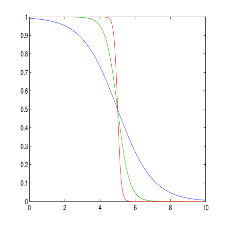
Figure 6: Illustration of the FD distribution. As $T$ decreases, the curve becomes closer to $\bar{n}_{r}=u(\mu-\epsilon_{r})$, where $u(\cdot)$ is the unit step function.

4.2 FD Statistics From the Grand–Canonical Ensemble

Thanks to the principle of ensemble equivalence, an alternative, simpler derivation of the FD distribution results from the use of the grand–canonical ensemble. Beginning from the canonical partition function

$$Z_{N}(\beta)=\sum_{N_{1}=0}^{1}\sum_{N_{2}=0}^{1}\ldots\delta\left(\sum_{r}N_{r}=N\right)e^{-\beta\sum_{r}N_{r}\epsilon_{r}},$$ (4.2.1)

we pass to the grand–canonical ensemble in the following manner:

$$\Xi(\beta,\mu) = \sum_{N=0}^{\infty}e^{\beta\mu N}\sum_{N_{1}=0}^{1}\sum_{N_{2}=0}^{1}\ldots\delta\left(\sum_{r}N_{r}=N\right)e^{-\beta\sum_{r}N_{r}\epsilon_{r}}$$ (4.2.2)

$$= \sum_{N=0}^{\infty}\sum_{N_{1}=0}^{1}\sum_{N_{2}=0}^{1}\ldots e^{\beta\mu\sum_{r}N_{r}}\delta\left(\sum_{r}N_{r}=N\right)e^{-\beta\sum_{r}N_{r}\epsilon_{r}}$$

$$= \sum_{N=0}^{\infty}\sum_{N_{1}=0}^{1}\sum_{N_{2}=0}^{1}\ldots\delta\left(\sum_{r}N_{r}=N\right)e^{\beta\sum_{r}N_{r}(\mu-\epsilon_{r})}$$

$$= \sum_{N_{1}=0}^{1}\sum_{N_{2}=0}^{1}\ldots\left[\sum_{N=0}^{\infty}\delta\left(\sum_{r}N_{r}=N\right)\right]e^{\beta\sum_{r}N_{r}(\mu-\epsilon_{r})}$$

$$= \sum_{N_{1}=0}^{1}\sum_{N_{2}=0}^{1}\ldots e^{\beta\sum_{r}N_{r}(\mu-\epsilon_{r})}$$

$$= \prod_{r}\left[\sum_{N_{r}=0}^{1}e^{\beta N_{r}(\mu-\epsilon_{r})}\right]$$

$$= \prod_{r}\left[1+e^{\beta(\mu-\epsilon_{r})}\right].$$

Note that this product form of the grand partition function means that under the grand–canonical ensemble the binary random variables $\{N_{r}\}$ are statistically independent, i.e.,

$$P(N_{1},N_{2},\ldots)=\prod_{r}P_{r}(N_{r})$$ (4.2.3)

where

$$P_{r}(N_{r})=\frac{e^{\beta N_{r}(\mu-\epsilon_{r})}}{1+e^{\beta(\mu-\epsilon_{r})}},~{}~{}~{}~{}~{}N_{r}=0,1,~{}~{}~{}~{}~{}r=1,2,\ldots.$$ (4.2.4)

Thus,

$$\bar{N}_{r}=\mbox{Pr}\{N_{r}=1\}=\frac{e^{(\mu-\epsilon_{r})/kT}}{1+e^{(\mu-\epsilon_{r})/kT}}=\frac{1}{e^{(\epsilon_{r}-\mu)/kT}+1}.$$ (4.2.5)

4.3 The Fermi Energy

Let us now examine what happens if the system is cooled to the absolute zero ($T\to 0$). It should be kept in mind that the chemical potential $\mu$ depends on $T$, so let $\mu_{0}$ be the chemical potential at $T=0$. It is readily seen that $\bar{N}_{r}$ approaches as step function (see Fig. 6), namely, all energy levels $\{\epsilon_{r}\}$ below $\mu_{0}$ are occupied ($\bar{N}_{r}\approx 1$) by a fermion, whereas all those that are above $\mu_{0}$ are empty ($\bar{N}_{r}\approx 0$). The explanation is simple: Pauli’s exclusion principle does not allow all particles to reside at the ground state at $T=0$ since then many of them would have occupied the same quantum state. The minimum energy of the system that can possibly be achieved is when all energy levels are filled up, one by one, starting from the ground state up to some maximum level, which is exactly $\mu_{0}$. This explains why even at the absolute zero, fermions have energy. The maximum occupied energy level in a gas of non–interacting fermions at the absolute zero is called the Fermi energy, which we shall denote by $\epsilon_{F}$. Thus, $\mu_{0}=\epsilon_{F}$, and then the FD distribution at very low temperatures is approximately

$$\bar{N}_{r}=\frac{1}{e^{(\epsilon_{r}-\epsilon_{F})/kT}+1}.$$ (4.3.1)

We next take a closer look on the FD distribution, taking into account the density of states. Consider a metal box of dimensions $L_{x}\times L_{y}\times L_{z}$ and hence volume $V=L_{x}L_{y}L_{z}$. The energy level associated with quantum number $(l_{x},l_{y},l_{z})$ is given by

$$\epsilon_{l_{x},l_{y},l_{z}}=\frac{\pi^{2}\hbar^{2}}{2m}\left(\frac{l_{x}^{2}}{L_{x}^{2}}+\frac{l_{y}^{2}}{L_{y}^{2}}+\frac{l_{z}^{2}}{L_{z}^{2}}\right)=\frac{\hbar^{2}}{2m}(k_{x}^{2}+k_{y}^{2}+k_{z}^{2}),$$ (4.3.2)

where the $k$’s are the wave numbers pertaining to the various solutions of the Schrödinger equation. First, we would like to count how many quantum states $\{(l_{x},l_{y},l_{z})\}$ give rise to energy between $\epsilon$ and $\epsilon+\mbox{d}\epsilon$. We denote this number by $g(\epsilon)\mbox{d}\epsilon$, where $g(\epsilon)$ is the density of states.

$$g(\epsilon)\mbox{d}\epsilon = \sum_{l_{x},l_{y},l_{z}}1\left\{\frac{2m\epsilon}{\hbar^{2}}\leq\frac{\pi^{2}l_{x}^{2}}{L_{x}^{2}}+\frac{\pi^{2}l_{y}^{2}}{L_{y}^{2}}+\frac{\pi^{2}l_{z}^{2}}{L_{z}^{2}}\leq\frac{2m(\epsilon+\mbox{d}\epsilon)}{\hbar^{2}}\right\}$$ (4.3.3)

$$\approx \frac{L_{x}L_{y}L_{z}}{\pi^{3}}\cdot\mbox{Vol}\left\{\vec{\mbox{\boldmath$k$}}:~{}\frac{2m\epsilon}{\hbar^{2}}\leq\|\vec{\mbox{\boldmath$k$}}\|^{2}\leq\frac{2m(\epsilon+\mbox{d}\epsilon)}{\hbar^{2}}\right\}$$

$$= \frac{V}{\pi^{3}}\cdot\mbox{Vol}\left\{\vec{\mbox{\boldmath$k$}}:~{}\frac{2m\epsilon}{\hbar^{2}}\leq\|\vec{\mbox{\boldmath$k$}}\|^{2}\leq\frac{2m(\epsilon+\mbox{d}\epsilon)}{\hbar^{2}}\right\}.$$

A volume element pertaining to a given value of $K=\|\vec{\mbox{\boldmath$k$}}\|$ ($\vec{\mbox{\boldmath$k$}}$ being $k_{x}\hat{x}+k_{y}\hat{y}+k_{z}\hat{z}$) is given by $\mbox{d}K$ times the surface area of sphere of radius $K$, namely, $4\pi K^{2}\mbox{d}K$, but it has to be divided by $8$, to account for the fact that the components of $\vec{\mbox{\boldmath$k$}}$ are positive. I.e., it is $\frac{\pi}{2}K^{2}\mbox{d}K$. From eq. (4.3.2), we have $\epsilon=\hbar^{2}K^{2}/2m$, and so

$$K^{2}\mbox{d}K=\frac{2m\epsilon}{\hbar^{2}}\cdot\frac{1}{2\hbar}\sqrt{\frac{2m}{\epsilon}}\mbox{d}\epsilon=\frac{\sqrt{2\epsilon m^{3}}\mbox{d}\epsilon}{\hbar^{3}}$$ (4.3.4)

Therefore, combining the above, we get

$$g(\epsilon)=\frac{\sqrt{2\epsilon m^{3}}V}{2\pi^{2}\hbar^{3}}.$$ (4.3.5)

For electrons, spin values of $\pm 1/2$ are allowed, so this density should be doubled, and so

$$g_{e}(\epsilon)=\frac{\sqrt{2\epsilon m^{3}}V}{\pi^{2}\hbar^{3}}.$$ (4.3.6)

Approximating the equation of the constraint on the total number of electrons, we get

$$N_{e} = \sum_{r}\frac{1}{e^{(\epsilon_{r}-\epsilon_{F})/kT}+1}$$ (4.3.7)

$$\approx \frac{\sqrt{2m^{3}}V}{\pi^{2}\hbar^{3}}\cdot\int_{0}^{\infty}\frac{\sqrt{\epsilon}\mbox{d}\epsilon}{e^{(\epsilon-\epsilon_{F})/kT}+1}$$

$$\approx \frac{\sqrt{2m^{3}}V}{\pi^{2}\hbar^{3}}\cdot\int_{0}^{\epsilon_{F}}\sqrt{\epsilon}\mbox{d}\epsilon~{}~{}~{}~{}~{}T\approx 0$$

$$= \frac{\sqrt{2m^{3}}V}{\pi^{2}\hbar^{3}}\cdot\frac{2\epsilon_{F}^{3/2}}{3}$$

which easily leads to the following simple formula for the Fermi energy:

$$\epsilon_{F}=\frac{\hbar^{2}}{2m}\left(\frac{3\pi^{2}N_{e}}{V}\right)^{2/3}=\frac{\hbar^{2}}{2m}(3\pi^{2}\rho_{e})^{2/3},$$ (4.3.8)

where $\rho_{e}$ is the electron density. In most metals $\epsilon_{F}$ is about the order of 5–10 electron–volts (eV’s), whose equivalent temperature $T_{F}=\epsilon_{F}/k$ (the Fermi temperature) is of the order of magnitude of $100,000^{o}$K. So the Fermi energy is much larger than $kT$ in laboratory conditions. In other words, electrons in a metal behave like a gas at an extremely high temperature. This means that the internal pressure in metals (the Fermi pressure) is huge and that’s a reason why metals are almost incompressible. This kind of pressure also stabilizes a neutron star (a Fermi gas of neutrons) or a white dwarf star (a Fermi gas of electrons) against the inward pull of gravity, which would ostensibly collapse the star into a Black Hole. Only when a star is sufficiently massive to overcome the degeneracy pressure can it collapse into a singularity.

Exercise 4.2: Derive an expression for $\left<\epsilon^{n}\right>$ of an electron near $T=0$, in terms of $\epsilon_{F}$.

4.4 Useful Approximations of Fermi Integrals

Before considering applications, it will be instructive to develop some useful approximations for integrals associated with the Fermi function

$$f(\epsilon)\stackrel{{\scriptstyle\Delta}}{{=}}\frac{1}{e^{(\epsilon-\mu)/kT}+1}.$$ (4.4.1)

For example, if we wish to calculate the average energy, we have to deal with an integral like

$$\int_{0}^{\infty}\epsilon^{3/2}f(\epsilon)\mbox{d}\epsilon.$$

Consider then, more generally, an integral of the form

$$I_{n}=\int_{0}^{\infty}\epsilon^{n}f(\epsilon)\mbox{d}\epsilon.$$

Upon integrating by parts, we readily have

$$I_{n} = f(\epsilon)\cdot\frac{\epsilon^{n+1}}{n+1}\bigg{|}_{0}^{\infty}-\frac{1}{n+1}\int_{0}^{\infty}\epsilon^{n+1}f^{\prime}(\epsilon)\mbox{d}\epsilon$$ (4.4.2)

$$= -\frac{1}{n+1}\int_{0}^{\infty}\epsilon^{n+1}f^{\prime}(\epsilon)\mbox{d}\epsilon$$

Changing variables to $x=(\epsilon-\mu)/kT$,

$$I_{n} = -\frac{1}{n+1}\int_{-\mu/kT}^{\infty}(\mu+kTx)^{n+1}\phi^{\prime}(x)\mbox{d}x$$ (4.4.3)

$$\approx -\frac{\mu^{n+1}}{n+1}\int_{-\infty}^{\infty}\left(1+\frac{kTx}{\mu}\right)^{n+1}\phi^{\prime}(x)\mbox{d}x,$$

where we have introduced the scaled version of $f$, which is $\phi(x)=f(\mu+kTx)=1/(e^{x}+1)$ and $\phi^{\prime}$ is its derivative, and where in the second line we are assuming $\mu\gg kT$. Applying the Taylor series expansion to the binomial term (recall that $n$ is not necessarily integer), and using the symmetry of $\phi^{\prime}$ around the origin, we have

$$I_{n} = -\frac{\mu^{n+1}}{n+1}\int_{-\infty}^{\infty}\left[1+(n+1)\frac{kTx}{\mu}+\frac{n(n+1)}{2}\left(\frac{kTx}{\mu}\right)^{2}+\ldots\right]\phi^{\prime}(x)\mbox{d}x$$ (4.4.4)

$$= -\frac{\mu^{n+1}}{n+1}\left[\int_{-\infty}^{\infty}\phi^{\prime}(x)\mbox{d}x+\frac{n(n+1)}{2}\left(\frac{kT}{\mu}\right)^{2}\int_{-\infty}^{\infty}x^{2}\phi^{\prime}(x)\mbox{d}x+\cdot\cdot\cdot\right]$$

$$\approx \frac{\mu^{n+1}}{n+1}\left[1+\frac{n(n+1)\pi^{2}}{6}\left(\frac{kT}{\mu}\right)^{2}\right]$$

where the last line was obtained by calculating the integral of $x^{2}\phi^{\prime}(x)$ using a power series expansion. Note that this series contains only even powers of $kT/\mu$, thus the convergence is rather fast. Let us now repeat the calculation of eq. (4.3.7), this time at $T>0$.

$$\rho_{e} \approx \frac{\sqrt{2m^{3}}}{\pi^{2}\hbar^{3}}\cdot\int_{0}^{\infty}\frac{\sqrt{\epsilon}\mbox{d}\epsilon}{e^{(\epsilon-\mu)/kT}+1}$$ (4.4.5)

$$= \frac{\sqrt{2m^{3}}}{\pi^{2}\hbar^{3}}\cdot I_{1/2}$$

$$= \frac{\sqrt{2m^{3}}}{\pi^{2}\hbar^{3}}\cdot\frac{2}{3}\mu^{3/2}\left[1+\frac{\pi^{2}}{8}\left(\frac{kT}{\mu}\right)^{2}\right]$$

which gives

$$\epsilon_{F} = \mu\left[1+\frac{\pi^{2}}{8}\left(\frac{kT}{\mu}\right)^{2}\right]^{2/3}$$ (4.4.6)

$$\approx \mu\left[1+\frac{\pi^{2}}{12}\left(\frac{kT}{\mu}\right)^{2}\right]$$

$$= \mu+\frac{(\pi kT)^{2}}{12\mu}.$$

This relation between $\mu$ and $\epsilon_{F}$ can be easily inverted by solving a simple quadratic equation, which yields

$$\mu \approx \frac{\epsilon_{F}+\epsilon_{F}\sqrt{1-(\pi kT/\epsilon_{F})^{2}/3}}{2}$$ (4.4.7)

$$\approx \epsilon_{F}\left[1-\frac{\pi^{2}}{12}\cdot\left(\frac{kT}{\epsilon_{F}}\right)^{2}\right]$$

$$= \epsilon_{F}\left[1-\frac{\pi^{2}}{12}\cdot\left(\frac{T}{T_{F}}\right)^{2}\right]$$

Since $T/T_{F}\ll 1$ for all $T$ in the interesting range, we observe that the chemical potential depends extremely weakly on $T$. In other words, we can safely approximate $\mu\approx\epsilon_{F}$ for all relevant temperatures of interest. The assumption that $kT\ll\mu$ was found self–consistent with the result $\mu\approx\epsilon_{F}$.

Having established the approximation $\mu\approx\epsilon_{F}$, we can now calculate the average energy of the electron at an arbitrary temperature $T$:

$$\left<\epsilon\right> = \frac{\sqrt{2m^{3}}}{\pi^{2}\hbar^{3}\rho_{e}}\int_{0}^{\infty}\frac{\epsilon^{3/2}\mbox{d}\epsilon}{e^{(\epsilon-\epsilon_{F})/kT}+1}$$ (4.4.8)

$$= \frac{\sqrt{2m^{3}}}{\pi^{2}\hbar^{3}\rho_{e}}\cdot I_{3/2}$$

$$\approx \frac{\sqrt{2m^{3}}}{\pi^{2}\hbar^{3}\rho_{e}}\cdot\frac{2\epsilon_{F}^{5/2}}{5}\left[1+\frac{5\pi^{2}}{8}\left(\frac{T}{T_{F}}\right)^{2}\right]$$

$$= \frac{3\hbar^{2}}{10m}\cdot(3\pi^{2}\rho_{e})^{2/3}\cdot\left[1+\frac{5\pi^{2}}{8}\left(\frac{T}{T_{F}}\right)^{2}\right]$$

$$= \frac{3\epsilon_{F}}{5}\cdot\left[1+\frac{5\pi^{2}}{8}\left(\frac{T}{T_{F}}\right)^{2}\right]$$

Note that the dependence of the average per–particle energy on the temperature is drastically different from that of the ideal gas. While in the idea gas it was linear ($\left<\epsilon\right>=3kT/2$), here it is actually almost a constant, independent of the temperature (just like the chemical potential).

The same technique can be used, of course, to calculate any moment of the electron energy.

4.5 Applications of the FD Distribution

The FD distribution is at the heart of modern solid–state physics and semiconductor physics (see also, for example, [3, Section 4.5]) and indeed frequently encountered in related courses, like courses on semiconductor devices. It is also useful in understanding the physics of white dwarfs. We next briefly touch upon the very basics of conductance in solids (as a much more comprehensive treatment is given, of course, in other courses), as well as on two other applications: thermionic emission and photoelectric emission.

4.5.1 Electrons in a Solid

The structure of the electron energy levels in a solid are basically obtained using quantum–mechanical considerations. In the case of a crystal, this amounts to solving the Schrödinger equation in a periodic potential, stemming from the corresponding periodic lattice structure. Its idealized form, which ignores the size of each atom, is given by a train of equispaced Dirac delta functions. This is an extreme case of the so called Kronig–Penney model, where the potential function is a periodic rectangular on–off function (square wave function), and it leads to a certain band structure. In particular, bands of allowed energy levels are alternately interlaced with bands of forbidden energy levels. The Fermi energy level $\epsilon_{F}$, which depends on the overall concentration of electrons, may either fall in an allowed band or in a forbidden band. The former case is the case of a metal, whereas the latter case is the case of an insulator or a semiconductor (the difference being only how wide is the forbidden band in which $\epsilon_{F}$ lies). While in metals it is impossible to change $\epsilon_{F}$, in semiconductors, it is possible by doping.

A semiconductor can then be thought of as a system with electron orbitals grouped into two energy bands separated by an energy gap. The lower band is the valence band (where electrons are tied to their individual atoms) and the upper band is the conduction band, where they are free. In a pure semiconductor at $T=0$, all valence orbitals are occupied with electrons and all conduction orbitals are empty. A full band cannot carry any current so a pure semiconductor at $T=0$ is an insulator. In a pure semiconductor the Fermi energy is exactly in the middle of the gap between the valence band (where $f(\epsilon)$ is very close 1) and the conduction band (where $f(\epsilon)$ is very close to 0). Finite conductivity in a semiconductor follows either from the presence of electrons in the conduction band (conduction electrons) or from unoccupied orbitals in the valence band (holes).

Two different mechanisms give rise to conduction electrons and holes: The first is thermal excitation of electrons from the valence band to the conduction band, and the second is the presence of impurities that change the balance between the number of orbitals in the valence band and the number of electrons available to fill them.

We will not delve into this too much beyond this point, since this material is well–covered in other courses solid state physics. Here we just demonstrate the use of the FD distribution in order to calculate the density of charge carriers. The density of charge carriers $n$ of the conduction band is found by integrating up, from the conduction band edge $\epsilon_{C}$, the product of the density of states $g_{e}(\epsilon)$ and the FD distribution $f(\epsilon)$, i.e.,

$$n=\int_{\epsilon_{C}}^{\infty}\mbox{d}\epsilon\cdot g_{e}(\epsilon)f(\epsilon)=\frac{\sqrt{2m^{3}}}{\pi^{2}\hbar^{3}}\int_{\epsilon_{C}}^{\infty}\frac{\sqrt{\epsilon-\epsilon_{C}}\mbox{d}\epsilon}{e^{(\epsilon-\epsilon_{F})/kT}+1},$$ (4.5.1)

where here $m$ designates the effective mass of the electron and where we have taken the density of states to be proportional to $\sqrt{\epsilon-\epsilon_{C}}$ since $\epsilon_{C}$ is now the reference energy and only the difference $\epsilon-\epsilon_{C}$ goes for kinetic energy. For a semiconductor at room temperature, $kT$ is much smaller than the gap, and so

$$f(\epsilon)\approx e^{-(\epsilon-\epsilon_{F})/kT}$$ (4.5.2)

which yields the approximation

$$n \approx \frac{\sqrt{2m^{3}}}{\pi^{2}\hbar^{3}}\cdot e^{\epsilon_{F}/kT}\int_{\epsilon_{C}}^{\infty}\mbox{d}\epsilon\cdot\sqrt{\epsilon-\epsilon_{C}}\cdot e^{-\epsilon/kT}$$ (4.5.3)

$$= \frac{\sqrt{2m^{3}}}{\pi^{2}\hbar^{3}}\cdot e^{-(\epsilon_{C}-\epsilon_{F})/kT}\int_{0}^{\infty}\mbox{d}\epsilon\cdot\sqrt{\epsilon}e^{-\epsilon/kT}$$

$$= \frac{\sqrt{2(mkT)^{3}}}{\pi^{2}\hbar^{3}}\cdot e^{-(\epsilon_{C}-\epsilon_{F})/kT}\int_{0}^{\infty}\mbox{d}x\cdot\sqrt{x}e^{-x}$$

$$= \frac{\sqrt{\pi}}{2}\cdot\frac{\sqrt{2(mkT)^{3}}}{\pi^{2}\hbar^{3}}\cdot e^{-(\epsilon_{C}-\epsilon_{F})/kT}$$

$$= \frac{1}{4}\cdot\left(\frac{2mkT}{\pi\hbar^{2}}\right)^{3/2}\cdot e^{-(\epsilon_{C}-\epsilon_{F})/kT}.$$

We see then that the density of conduction electrons, and hence also the conduction properties, depend critically on the gap between $\epsilon_{C}$ and $\epsilon_{F}$. A similar calculation holds for the holes, of course.

4.5.2 Thermionic Emission^∗

If a refractory metal, like tungsten, is heated to a temperature of a few hundred degrees below the melting point, an electron emission can be drawn from it to a positive anode. From a quantum–mechanical viewpoint, the heated metal can be regarded as a potential well with finitely high walls determined by the surface potential barrier. Thus, some of the incident particles will have sufficient energy to surmount the surface barrier (a.k.a. the surface work function) and hence will be emitted. The work function $\phi$ varies between 2eV and 6eV for pure metals. The electron will not be emitted unless the energy component normal to the surface would exceed $\epsilon_{F}+\phi$. The excess energy beyond this threshold is in the form of translational kinetic energy which dictates the velocity away from the surface.

The analysis of this effect is made by transforming the energy distribution into a distribution in terms of the three component velocities $v_{x}$, $v_{y}$, $v_{z}$. We begin with the expression of the energy of a single electron

$$\epsilon=\frac{1}{2}m(v_{x}^{2}+v_{y}^{2}+v_{z}^{2})=\frac{\pi^{2}\hbar^{2}}{2m}\left(\frac{l_{x}^{2}}{L_{x}^{2}}+\frac{l_{y}^{2}}{L_{y}^{2}}+\frac{l_{z}^{2}}{L_{z}^{2}}\right).$$ (4.5.4)

Thus, $\mbox{d}v_{x}=h\mbox{d}l_{x}/(2mL_{x})$ and similar relations hold for two the other components, which together yield

$$\mbox{d}l_{x}\mbox{d}l_{y}\mbox{d}l_{z}=\left(\frac{m}{h}\right)^{3}V\mbox{d}v_{x}\mbox{d}v_{y}\mbox{d}v_{z},$$ (4.5.5)

where we have divided by 8 since every quantum state can be occupied by only one out of 8 combinations of the signs of the three component veocities. Thus, we can write the distribution function of the number of electrons in a cube $\mbox{d}v_{x}\times\mbox{d}v_{y}\times\mbox{d}v_{z}$ as

$$\mbox{d}N=2V\left(\frac{m}{h}\right)^{3}\frac{\mbox{d}v_{x}\mbox{d}v_{y}\mbox{d}v_{z}}{1+\exp\left\{\frac{1}{kT}\left[\frac{1}{2}m(v_{x}^{2}+v_{y}^{2}+v_{z}^{2})-\epsilon_{F}\right]\right\}},$$ (4.5.6)

where we have taken the chemical potential of the electron gas to be $\epsilon_{F}$, independently of temperature, as was justified in the previous subsection. Assuming that the surface is parallel to the YZ plane, the minimum escape velocity in the $x$–direction is $v_{0}=\sqrt{\frac{2}{m}(\epsilon_{F}+\phi)}$ and there are no restrictions on $v_{y}$ and $v_{z}$. The current along the $x$–direction is

$$I = \frac{\mbox{d}q}{\mbox{d}t}=\frac{q_{e}\mbox{d}N[\mbox{leaving the surface}]}{\mbox{d}t}$$ (4.5.7)

$$= \frac{q_{e}}{\mbox{d}t}\int_{v_{0}}^{\infty}\int_{-\infty}^{+\infty}\int_{-\infty}^{+\infty}\frac{v_{x}\mbox{d}t}{L_{x}}\cdot 2V\left(\frac{m}{h}\right)^{3}\frac{\mbox{d}v_{x}\mbox{d}v_{y}\mbox{d}v_{z}}{1+\exp\left\{\frac{1}{kT}\left[\frac{1}{2}m(v_{x}^{2}+v_{y}^{2}+v_{z}^{2})-\epsilon_{F}\right]\right\}}$$

$$= 2L_{y}L_{z}q_{e}\left(\frac{m}{h}\right)^{3}\int_{v_{0}}^{\infty}v_{x}\mbox{d}v_{x}\int_{-\infty}^{+\infty}\frac{\mbox{d}v_{y}\mbox{d}v_{z}}{1+\exp\left\{\frac{1}{kT}\left[\frac{1}{2}m(v_{x}^{2}+v_{y}^{2}+v_{z}^{2})-\epsilon_{F}\right]\right\}},$$

where the factor $v_{x}\mbox{d}t/L_{x}$ in the second line is the fraction of electrons close enough to the sufrace so as to be emitted within time $\mbox{d}t$. Thus, the current density (current per unity area) is

$$J=2q_{e}\left(\frac{m}{h}\right)^{3}\int_{v_{0}}^{\infty}\mbox{d}v_{x}\cdot v_{x}\int_{-\infty}^{+\infty}\int_{-\infty}^{+\infty}\frac{\mbox{d}v_{y}\mbox{d}v_{z}}{1+\exp\left\{\frac{1}{kT}\left[\frac{1}{2}m(v_{x}^{2}+v_{y}^{2}+v_{z}^{2})-\epsilon_{F}\right]\right\}}.$$ (4.5.8)

As for the inner double integral, transform to polar coordinates to obtain

$$\int_{-\infty}^{+\infty}\int_{-\infty}^{+\infty}\frac{\mbox{d}v_{y}\mbox{d}v_{z}}{1+\exp\left\{\frac{1}{kT}\left[\frac{1}{2}m(v_{x}^{2}+v_{y}^{2}+v_{z}^{2})-\epsilon_{F}\right]\right\}}$$ (4.5.9)

$$= 2\pi\int_{0}^{\infty}\frac{v_{yz}\mbox{d}v_{yz}}{1+e^{mv_{yz}^{2}/2kT}\cdot\exp\left[\frac{1}{kT}\left(\frac{1}{2}mv_{x}^{2}-\epsilon_{F}\right)\right]}$$

$$= \frac{2\pi kT}{m}\int_{0}^{\infty}\frac{\mbox{d}u}{1+\exp\left[\frac{1}{kT}\left(\frac{1}{2}mv_{x}^{2}-\epsilon_{F}\right)\right]\cdot e^{u}}~{}~{}~{}~{}~{}~{}~{}~{}~{}~{}~{}~{}~{}u=mv_{yz}^{2}/2kT$$

$$= \frac{2\pi kT}{m}\ln\left\{1+\exp\left[\frac{1}{kT}\left(\epsilon_{F}-\frac{1}{2}mv_{x}^{2}\right)\right]\right\}$$

which yields

$$J=\frac{4\pi m^{2}q_{e}kT}{h^{3}}\int_{v_{0}}^{\infty}\mbox{d}v_{x}\cdot v_{x}\ln\left\{1+\exp\left[\frac{1}{kT}\left(\epsilon_{F}-\frac{1}{2}mv_{x}^{2}\right)\right]\right\}.$$ (4.5.10)

Now, since normally $\phi\gg kT$, the exponent in the integrand is very small throughout the entire range of integration and so, it is safe to approximate it by $\ln(1+x)\approx x$, i.e.,

$$J \approx \frac{4\pi m^{2}q_{e}kT}{h^{3}}e^{\epsilon_{F}/kT}\int_{v_{0}}^{\infty}\mbox{d}v_{x}\cdot v_{x}e^{-mv_{x}^{2}/2kT}$$ (4.5.11)

$$= \frac{4\pi mq_{e}(kT)^{2}}{h^{3}}\exp\left\{\frac{1}{kT}\left(\epsilon_{F}-\frac{1}{2}mv_{0}^{2}\right)\right\}$$

$$= \frac{4\pi mq_{e}(kT)^{2}}{h^{3}}e^{-\phi/kT},$$

and thus we have obtained a simple expression for the density current as function of temperature. This result, which is known as the Richardson–Dushman equation, is in very good agreement with experimental evidence. Further discussion on this result can be found in [3] and [10].

4.5.3 Photoelectric Emission^∗

An analysis based on a similar line of thought applies also to the photoelectric emission, an effect where electrons are emitted from a metal as a result of radiation at frequency beyond a certain critical frequency $\nu_{0}$ (the Einstein threshold frequency), whose corresponding photon energy $h\nu_{0}$ is equal to the work function $\phi$. Here, the electron gains an energy amount of $h\nu$ from a photon, which helps to pass the energy barrier, and so the minimum velocity of emission, after excitation by a photon of energy $h\nu$ is given by

$$h\nu+\frac{1}{2}mv_{0}^{2}=\epsilon_{F}+\phi=\epsilon_{F}+h\nu_{0}.$$ (4.5.12)

Let $\alpha$ denote the probability that a photon actually excites an electron. Then, similarly as in the previous subsection,

$$J=\alpha\cdot\frac{4\pi m^{2}q_{e}kT}{h^{3}}\int_{v_{0}}^{\infty}\mbox{d}v_{x}\cdot v_{x}\ln\left\{1+\exp\left[\frac{1}{kT}\left(\epsilon_{F}-\frac{1}{2}mv_{x}^{2}\right)\right]\right\}.$$ (4.5.13)

where this time

$$v_{0}=\sqrt{\frac{2}{m}[\epsilon_{F}+h(\nu_{0}-\nu)]}.$$ (4.5.14)

Changing the integration variable to

$$x=\frac{1}{kT}\left[\frac{1}{2}mv_{x}^{2}+h(\nu-\nu_{0})-\epsilon_{F}\right],$$

we can write the last integral as

$$J=\alpha\cdot\frac{4\pi mq_{e}(kT)^{2}}{h^{3}}\int_{0}^{\infty}\mbox{d}x\ln\left\{1+\exp\left[\frac{h(\nu-\nu_{0})}{kT}-x\right]\right\}\mbox{d}x.$$ (4.5.15)

Now, let us denote

$$\Delta=\frac{h(\nu-\nu_{0})}{kT}.$$ (4.5.16)

Integrating by parts (twice), we have

$$\int_{0}^{\infty}\mbox{d}x\ln(1+e^{\Delta-x}) = \int_{0}^{\infty}\frac{x\mbox{d}x}{e^{x-\Delta}+1}$$ (4.5.17)

$$= \frac{1}{2}\int_{0}^{\infty}\frac{x^{2}e^{x-\Delta}\mbox{d}x}{(e^{x-\Delta}+1)^{2}}\stackrel{{\scriptstyle\Delta}}{{=}}f(e^{\Delta}).$$

For $h(\nu-\nu_{0})\gg kT$, we have $e^{\Delta}\gg 1$, and then it can be shown (using the same technique as in Subsection 4.4) that $f(e^{\Delta})\approx\Delta^{2}/2$, which gives

$$J=\alpha\cdot\frac{2\pi mq_{e}}{h}(\nu-\nu_{0})^{2}$$ (4.5.18)

independently of $T$. In other words, when the energy of light quantum is much larger than the thermal energy $kT$, temperature becomes irrelevant. At the other extreme of very low frequency, where $h(\nu_{0}-\nu)\gg kT$, and then $e^{\Delta}\ll 1$, we have $f(e^{\Delta})\approx e^{\Delta}$, and then

$$J=\alpha\cdot\frac{4\pi mq_{e}(kT)^{2}}{h^{3}}e^{(h\nu-\phi)/kT}$$ (4.5.19)

which is like the thermionic current density, enhanced by a photon factor $e^{h\nu/kT}$.

5 Quantum Statistics – the Bose–Einstein Distribution

The general description of bosons was provided in the introductory paragraphs of Chapter 4. As said, the crucial difference between bosons and fermions is that in the case of bosons, Pauli’s exclusion principle does not apply. In this chapter, we study the statistical mechanics of bosons.

5.1 Combinatorial Derivation of the BE Statistics

We use the same notation as in Chapter 4. Again, we are partitioning the energy levels $\epsilon_{1},\epsilon_{2},\ldots$ into groups, labeled by $s=1,2,\ldots$, where in group no. $s$, where the representative energy is $\hat{\epsilon}_{s}$, there are $G_{s}$ quantum states. As before, a microstate is defined in terms of the combination of occupation numbers $\{\hat{N}_{s}\}$ and $\Omega(\hat{N}_{1},\hat{N}_{2},\ldots)=\prod_{s}\Omega_{s}(\hat{N}_{s})$, but now we need a different estimate of each factor $\Omega_{s}(\hat{N}_{s})$, since now there are no restrictions on the occupation numbers of the quantum states.

In how many ways can one partition $\hat{N}_{s}$ particles among $G_{s}$ quantum states? Imagine that the $\hat{N}_{s}$ particles of group no. $s$ are arranged along a straight line. By means of $G_{s}-1$ partitions we can divide these particles into $G_{s}$ different subsets corresponding to the various states in that group. In fact, we have a total of $(\hat{N}_{s}+G_{s}-1)$ elements, $\hat{N}_{s}$ of them are particles and the remaining $(G_{s}-1)$ are partitions (see Fig. 7).

\begin{picture}(4869.0,570.0)(379.0,-123.0)\end{picture}

Figure 7: $\hat{N}_{s}$ particles and $G_{s}-1$ partitions.

In how many distinct ways can we configure them? The answer is simple:

$$\Omega_{s}(\hat{N}_{s})=\frac{(\hat{N}_{s}+G_{s}-1)!}{\hat{N}_{s}!(G_{s}-1)!}.$$ (5.1.1)

On the account that $G_{s}\gg 1$, the $-1$ can be safely neglected, and we might as well write instead

$$\Omega_{s}(\hat{N}_{s})=\frac{(\hat{N}_{s}+G_{s})!}{\hat{N}_{s}!G_{s}!}.$$ (5.1.2)

Repeating the same derivation as in Subsection 4.1, but with the above assignment for $\Omega_{s}(\hat{N}_{s})$, we get by Stirling’s formula:

$$\ln\Omega_{s}(\hat{N}_{s})\approx(\hat{N}_{s}+G_{s})h_{2}\left(\frac{G_{s}}{\hat{N}_{s}+G_{s}}\right),$$ (5.1.3)

and so the free energy is now

$$F\approx\sum_{s}\left[\hat{N}_{s}\hat{\epsilon}_{s}-kT(\hat{N}_{s}+G_{s})h_{2}\left(\frac{\hat{N}_{s}}{\hat{N}_{s}+G_{s}}\right)\right],$$ (5.1.4)

which again, should be minimized s.t. the constraint $\sum_{s}\hat{N}_{s}=N$. Upon carrying out the minimization of the corresponding Lagrangian (see Subsection 4.1), we arrive at the following result for the most probable occupation numbers:

$$\hat{N}_{s}=\frac{G_{s}}{e^{\beta(\hat{\epsilon}_{s}-\mu)}-1}$$ (5.1.5)

or, moving back to the original occupation numbers,

$$\bar{N}_{r}=\frac{1}{e^{\beta(\epsilon_{r}-\mu)}-1},$$ (5.1.6)

where $\mu$ is again the Lagrange multiplier, which has the meaning of the chemical potential. This is Bose–Einstein (BE) distribution. As we see, the formula is very similar to that of the FD distribution, the only difference is that in the denominator, $+1$ is replaced by $-1$. Surprisingly enough, this is a crucial difference that makes the behavior of bosons drastically different from that of fermions. Note that for this expression to make sense, $\mu$ must be smaller than the ground energy $\epsilon_{1}$, otherwise the denominator either vanishes or becomes negative. If the ground–state energy is zero, this means $\mu<0$.

5.2 Derivation Using the Grand–Canonical Ensemble

As in Subsection 4.2, an alternative derivation can be carried out using the grand–canonical ensemble. The only difference is that now, the summations over $\{N_{r}\}$, are not only over $\{0,1\}$ but over all non–negative integers. In particular,

$$\Xi(\beta,\mu)=\prod_{r}\left[\sum_{N_{r}=0}^{\infty}e^{\beta N_{r}(\mu-\epsilon_{r})}\right],$$ (5.2.1)

Of course, here too, for convergence of each geometric series, we must assume $\mu<\epsilon_{1}$, and then the result is

$$\Xi(\beta,\mu)=\prod_{r}\frac{1}{1-e^{\beta(\mu-\epsilon_{r})}}.$$ (5.2.2)

Here, under the grand–canonical ensemble, $N_{1},N_{2},\ldots$ are independent geometric random variables with distributions

$$P_{r}(N_{r})=[1-e^{\beta(\mu-\epsilon)}]e^{\beta N_{r}(\mu-\epsilon_{r})}~{}~{}~{}~{}~{}N_{r}=0,1,2,\ldots,~{}~{}~{}r=1,2,\ldots$$ (5.2.3)

Thus, $\bar{N}_{r}$ is just the expectation of this geometric random variable, which is readily found to be as in eq. (5.1.6).

5.3 Bose–Einstein Condensation

In analogy to the FD case, here too, the chemical potential $\mu$ is determined from the constraint on the total number of particles. In this case, it reads

$$\sum_{r}\frac{1}{e^{\beta(\epsilon_{r}-\mu)}-1}=N.$$ (5.3.1)

Taking into account the density of states in a potential well of sizes $L_{x}\times L_{y}\times L_{z}$ (as was done in Chapter 4), in the continuous limit, this yields

$$\rho=\frac{\sqrt{2m^{3}}}{2\pi^{2}\hbar^{3}}\cdot\int_{0}^{\infty}\frac{\sqrt{\epsilon}\mbox{d}\epsilon}{e^{(\epsilon-\mu)/kT}-1}.$$ (5.3.2)

At this point, an important peculiarity should be discussed. Consider eq. (5.3.2) and suppose that we are cooling the system. As $T$ decreases, $\mu$ must adjust in order to keep eq. (5.3.2) holding since the number of particles must be preserved. In particular, as $T$ decreases, $\mu$ must increase, yet it must be negative. The point is that even for $\mu=0$, which is the maximum allowed value of $\mu$, the integral at the r.h.s. of (5.3.2) is finite as the density of states is proportional to $\sqrt{\epsilon}$ and hence balances the ‘explosion’ of the BE integral near $\epsilon=0$. Let us define then

$$\varrho(T)\stackrel{{\scriptstyle\Delta}}{{=}}\frac{\sqrt{2m^{3}}}{2\pi^{2}\hbar^{3}}\cdot\int_{0}^{\infty}\frac{\sqrt{\epsilon}\mbox{d}\epsilon}{e^{\epsilon/kT}-1}$$ (5.3.3)

and let $T_{c}$ be the solution to the equation $\varrho(T)=\rho$, which can be found as follows. By changing the integration variable to $z=\epsilon/kT$, we can rewrite the r.h.s. as

$$\varrho(T)=\left(\frac{mkT}{2\pi\hbar^{2}}\right)^{3/2}\left\{\frac{2}{\sqrt{\pi}}\int_{0}^{\infty}\frac{\sqrt{z}\mbox{d}z}{e^{z}-1}\right\}\approx 2.612\cdot\left(\frac{mkT}{2\pi\hbar^{2}}\right)^{3/2},$$ (5.3.4)

where the constant $2.612$ is the numerical value of the expression in the curly brackets. Thus,

$$T_{c}\approx 0.5274\cdot\frac{2\pi\hbar^{2}}{mk}\cdot\rho^{2/3}=3.313\cdot\frac{\hbar^{2}\rho^{2/3}}{mk}$$ (5.3.5)

The problem is that for $T<T_{c}$, eq. (5.3.2) can no longer be solved by any non–positive value of $\mu$. So what happens below $T_{c}$?

The root of the problem is in the passage from the discrete sum over $r$ to the integral over $\epsilon$. The paradox is resolved when it is understood that below $T_{c}$, the contribution of $\epsilon=0$ should be separated from the integral. That is, the correct form is

$$N=\frac{1}{e^{-\mu/kT}-1}+\frac{\sqrt{2m^{3}}V}{2\pi^{2}\hbar^{3}}\cdot\int_{0}^{\infty}\frac{\sqrt{\epsilon}\mbox{d}\epsilon}{e^{(\epsilon-\mu)/kT}-1}.$$ (5.3.6)

or, after dividing by $V$,

$$\rho=\rho_{0}+\frac{\sqrt{2m^{3}}}{2\pi^{2}\hbar^{3}}\cdot\int_{0}^{\infty}\frac{\sqrt{\epsilon}\mbox{d}\epsilon}{e^{(\epsilon-\mu)/kT}-1},$$ (5.3.7)

where $\rho_{0}$ is the density of ground–state particles, and now the integral accommodates the contribution of all particles with strictly positive energy. Now, for $T<T_{c}$, we simply have $\rho_{0}=\rho-\varrho(T)$, which means that a macroscopic fraction of the particles condensate at the ground state. This phenomenon is called Bose–Einstein condensation. Note that for $T<T_{c}$,

$$\rho_{0} = \rho-\varrho(T)$$ (5.3.8)

$$= \varrho(T_{c})-\varrho(T)$$

$$= \varrho(T_{c})\left[1-\frac{\varrho(T)}{\varrho(T_{c})}\right]$$

$$= \varrho(T_{c})\left[1-\left(\frac{T}{T_{c}}\right)^{3/2}\right]$$

$$= \rho\left[1-\left(\frac{T}{T_{c}}\right)^{3/2}\right]$$

which gives a precise characterization of the condensation as a function of temperature. It should be pointed out that $T_{c}$ is normally extremely low.

One might ask why does the point $\epsilon=0$ require special caution when $T<T_{c}$, but doesn’t require such caution for $T>T_{c}$? The answer is that for $T>T_{c}$, $\rho_{0}=1/V[e^{-\mu/kT}-1]$ tends to zero in the thermodynamic limit ($V\to\infty$) since $\mu<0$. However, as $T\to T_{c}$, $\mu\to 0$, and $\rho_{0}$ becomes singular.

It is instructive to derive the pressure exerted by the ideal Boson gas for $T<T_{c}$. This can be obtained from the grand partition function

$$\ln\Xi = -\sum_{r}\ln(1-e^{-\epsilon_{r}/kT})~{}~{}~{}~{}~{}~{}~{}~{}~{}~{}~{}~{}~{}~{}~{}~{}~{}(\mu=0)$$ (5.3.9)

$$\sim -\frac{\sqrt{2m^{3}}V}{2\pi^{2}\hbar^{3}}\int_{0}^{\infty}\mbox{d}\epsilon\cdot\sqrt{\epsilon}\ln(1-e^{-\epsilon/kT})$$

$$= -\frac{\sqrt{2m^{3}}(kT)^{3/2}V}{2\pi^{2}\hbar^{3}}\int_{0}^{\infty}\mbox{d}x\cdot\sqrt{x}\ln(1-e^{-x}),$$

where integral over $x$ (including the minus sign) is just a positive constant $C$ that we won’t bother to calculate here. Now,

$$P=\lim_{V\to\infty}\frac{kT\ln\Xi}{V}=\frac{C\sqrt{2m^{3}}(kT)^{5/2}}{2\pi^{2}\hbar^{3}}.$$ (5.3.10)

We see that the pressure is independent of the density $\rho$ (compare with the ideal gas where $P=\rho kT$). This is because the condensed particles do not contribute to the pressure. What matters is only the density of those with positive energy, and this density in turn depends only on $T$.

Exercise 5.4: Why don’t fermions condensate? What changes in the last derivation?

Exercise 5.5: The last derivation was in three dimensions ($d=3$). Modify the derivation of the BE statistics to apply to a general dimension $d$, taking into account the dependence of the density of states upon $d$. For which values of $d$ bosons condensate?

5.4 Black–Body Radiation

One of the important applications of the BE statistics is to investigate the equilibrium properties of black–body radiation. All bodies emit electromagnetic radiation whenever at positive temperature, but normally, this radiation is not in thermal equilibrium. If we consider the radiation within an opaque enclosure whose walls are maintained at temperature $T$ then radiation and walls together arrive at thermal equilibrium and in this state, the radiation has certain important properties. In order to study this equilibrium radiation, one creates a small hole in the walls of the enclosure, so that it will not disturb the equilibrium of the cavity and then the emitted radiation will have the same properties as the cavity radiation, which in turn are the same as the radiation properties of a black body – a body that perfectly absorbs all the radiation falling on it. The temperature of the black body is $T$ as well, of course. In this section, we study these radiation properties using BE statistics.

We consider then a radiation cavity of volume $V$ and temperature $T$. Historically, Planck (1900) viewed this system as an assembly of harmonic oscillators with quantized energies $(n+1/2)\hbar\omega$, $n=0,1,2,\ldots$, where $\omega$ is the angular frequency of the oscillator. An alternative point of view is as an ideal gas of identical and indistinguishable photons, each one with energy $\hbar\omega$. Photons have integral spin and hence are bosons, but they have zero mass and zero chemical potential when they interact with a black–body. The reason is that there is no constraint that their total number would be conserved (they are emitted and absorbed in the black–body material with which they interact). Since in equilibrium $F$ should be minimum, then $(\partial F/\partial N)_{T,V}=0$. But $(\partial F/\partial N)_{T,V}=\mu$. and so, $\mu=0$. It follows then that distribution of photons across the quantum states obeys BE statistics with $\mu=0$, that is

$$\bar{N}_{\omega}=\frac{1}{e^{\hbar\omega/kT}-1}.$$ (5.4.1)

The calculation of the density of states here is somewhat different from the one in Subsection 4.3. Earlier, we considered a particle with positive mass $m$, whose kinetic energy is $\|\vec{\mbox{\boldmath$p$}}\|^{2}/2m=\hbar^{2}\|\vec{\mbox{\boldmath$k$}}\|^{2}/2m$, whereas now we are talking about a photon whose rest mass is zero and whose energy is $\hbar\omega=\hbar\|\vec{k}\|c=\|\vec{\mbox{\boldmath$p$}}\|c$ ($c$ being the speed of light), so the dependence on $\|\vec{\mbox{\boldmath$k$}}\|$ is now linear rather than quadratic. This is a relativistic effect.

Assuming that $V$ is large enough, we can pass to the continuous approximation. The number of oscillatory modes for which a wave–vector $\vec{\mbox{\boldmath$k$}}$ resides in an infinitesimal cube $\mbox{d}^{3}\vec{\mbox{\boldmath$k$}}=\mbox{d}k_{x}\mbox{d}k_{y}\mbox{d}k_{z}$ is $V\cdot 4\pi\|\vec{\mbox{\boldmath$k$}}\|^{2}\mbox{d}\|\vec{\mbox{\boldmath$k$}}\|/(2\pi)^{3}$, as in phase space of position and momentum, it is

$$V4\pi\|\vec{\mbox{\boldmath$p$}}\|^{2}\mbox{d}\|\vec{\mbox{\boldmath$p$}}\|/h^{3}=V4\pi\|\hbar\vec{\mbox{\boldmath$k$}}\|^{2}\mbox{d}\|\vec{\hbar\mbox{\boldmath$k$}}\|/(2\pi\hbar)^{3}=V\cdot 4\pi\|\vec{\mbox{\boldmath$k$}}\|^{2}\mbox{d}\|\vec{\mbox{\boldmath$k$}}\|/(2\pi)^{3}.$$ (5.4.2)

Using the relation $\omega=c\|\vec{\mbox{\boldmath$k$}}\|$ and doubling the above expression (for two directions of polarization), we have that the total number of quantum states of a photon in the range $[\omega,\omega+\mbox{d}\omega]$ is $V\omega^{2}\mbox{d}\omega/\pi^{2}c^{3}$. Thus, the number of photons in this frequency range is

$$\mbox{d}N_{\omega}=\frac{V}{\pi^{2}c^{3}}\cdot\frac{\omega^{2}\mbox{d}\omega}{e^{\hbar\omega/kT}-1}.$$ (5.4.3)

The contribution of this to the energy is

$$\mbox{d}E_{\omega}=\hbar\omega\mbox{d}N_{\omega}=\frac{\hbar V}{\pi^{2}c^{3}}\cdot\frac{\omega^{3}\mbox{d}\omega}{e^{\hbar\omega/kT}-1}$$ (5.4.4)

This expression for the spectrum of black–body radiation is known as Planck’s law.

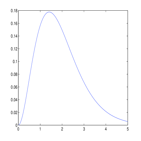
Figure 8: Illustration of Planck’s law. The energy density per unit frequency as a function of frequency.

Exercise 5.6: Write Planck’s law in terms of the wavelength $\mbox{d}E_{\lambda}$.

At low frequencies ($\hbar\omega\ll kT$), this gives

$$\mbox{d}E_{\omega}\approx\frac{kTV}{\pi^{2}c^{3}}\omega^{2}\mbox{d}\omega$$ (5.4.5)

which is the Rayleigh–Jeans law. This is actually the classic limit (see footnote at the Introduction to Chap. 4), obtained from multiplying $kT/2$ by the “number of waves.” In the other extreme of $\hbar\omega\gg kT$, we have

$$\mbox{d}E_{\omega}\approx\hbar\omega\mbox{d}N_{\omega}=\frac{\hbar V}{\pi^{2}c^{3}}\cdot\omega^{3}e^{-\hbar\omega/kT}\mbox{d}\omega,$$ (5.4.6)

which is Wien’s law. At low temperatures, this is an excellent approximation over a very wide range of frequencies. The frequency of maximum radiation is

$$\omega_{\max}=2.822\cdot\frac{kT}{\hbar},$$ (5.4.7)

namely, linear in temperature. This relation has immediate applications. For example, the sun is known to be a source of radiation, which with a good level of approximation, can be considered a black body. Using a spectrometer, one can measure the frequency $\omega_{\max}$ of maximum radiation, and estimate the sun’s surface temperature (from eq. (5.4.7)), to be $T\approx 5800^{\mbox{o}}K$.

Now, the energy density is

$$\frac{E}{V}=\frac{\hbar}{\pi^{2}c^{3}}\int_{0}^{\infty}\frac{\omega^{3}\mbox{d}\omega}{e^{\hbar\omega/kT}-1}=aT^{4}$$ (5.4.8)

where the second equality is obtained by changing the integration variable to $x=\hbar\omega/kT$ and then

$$a=\frac{\hbar}{\pi^{2}c^{3}}\left(\frac{k}{\hbar}\right)^{4}\int_{0}^{\infty}\frac{x^{3}\mbox{d}x}{e^{x}-1}=\frac{\pi^{2}k^{4}}{15\hbar^{3}c^{3}}.$$ (5.4.9)

The relation $E/V=aT^{4}$ is called the Stefan–Boltzmann law. The heat capacity in constant volume, $C_{V}=(\partial E/\partial T)_{V}$, is therefore proportional to $T^{3}$.

Exercise 5.7: Calculate $\rho$, the density of photons.

Additional thermodynamic quantities can now be calculated from the logarithm of the grand–canonical partition function

$$\ln\Xi=-\sum_{r}\ln[1-e^{-\hbar\omega_{r}/kT}]=-\frac{V}{\pi^{2}c^{3}}\int_{0}^{\infty}\mbox{d}\omega\cdot\omega^{2}\ln[1-e^{-\hbar\omega/kT}]$$ (5.4.10)

For example, the pressure of the photon gas can be calculated from

$$P = \frac{kT\ln\Xi}{V}$$ (5.4.11)

$$= -\frac{kT}{\pi^{2}c^{3}}\int_{0}^{\infty}\mbox{d}\omega\cdot\omega^{2}\ln[1-e^{-\hbar\omega/kT}]$$

$$= -\frac{(kT)^{4}}{\pi^{2}c^{3}\hbar^{3}}\int_{0}^{\infty}\mbox{d}x\cdot x^{2}\ln(1-e^{-x})$$

$$= \frac{1}{3}aT^{4}=\frac{E}{3V},$$

where the integral is calculated using integration by parts. Note that while in the ideal gas $P$ was only linear in $T$, here it is proportional to the fourth power of $T$. Note also that here, $PV=E/3$, which is different from the ideal gas, where $PV=2E/3$.

6 Interacting Particle Systems and Phase Transitions

In this chapter, we discuss systems with interacting particles. As we shall see, when the interactions among the particles are sufficiently significant, the system exhibits a certain collective behavior that, in the thermodynamic limit, may be subjected to phase transitions, i.e., abrupt changes in the behavior and the properties of the system in the presence of a gradual change in an external control parameter, like temperature, pressure, or magnetic field.

6.1 Introduction – Sources of Interaction

So far, we have dealt almost exclusively with systems that have additive Hamiltonians, ${\cal E}(\mbox{\boldmath$x$})=\sum_{i}{\cal E}(x_{i})$, which means, under the canonical ensemble, that the particles are statistically independent and there are no interactions among them: each particle behaves as if it was alone in the world. In Nature, of course, this is seldom really the case. Sometimes this is still a reasonably good approximation, but in many other cases, the interactions are appreciably strong and cannot be neglected. Among the different particles there could be many sorts of mutual forces, such as mechanical, electrical, or magnetic forces, etc. There could also be interactions that stem from quantum–mechanical effects: As described earlier, fermions must obey Pauli’s exclusion principle, which asserts that no quantum state can be populated by more than one particle. This gives rise to a certain mutual influence between particles. Another type of interaction stems from the fact that the particles are indistinguishable, so permutations between them are not considered as distinct states. For example, referring again to BE statistics of Chapter 5, had the $N$ particles been statistically independent, the resulting partition function would be

$$Z_{N}(\beta) =\left[\sum_{r}e^{-\beta\epsilon_{r}}\right]^{N}$$

$$=\sum_{N_{1},N_{2},\ldots}\delta\left(\sum_{r}N_{r}=N\right)\frac{N!}{\prod_{r}N_{r}!}\cdot\exp\left\{-\beta\sum_{r}N_{r}\epsilon_{r}\right\}$$ (6.1.1)

whereas in eq. (4.2.1) (but with summations extending over all integers $\{N_{r}\}$), the combinatorial factor, $N!/\prod_{r}N_{r}!$, that distinguishes between the various permutations among the particles, is absent. This introduces dependency, which physically means interaction. Indeed, in the case of the ideal boson gas, we have encountered the effect of Bose–Einstein condensation, which is actually a phase transition, and phase transitions can occur only in systems of interacting particles, as will be discussed in this chapter.

6.2 Models of Interacting Particles

The simplest forms of deviation from the purely additive Hamiltonian structure are those that consists, in addition to the individual energy terms, $\{{\cal E}(x_{i})\}$, also terms that depend on pairs, and/or triples, and/or even larger cliques of particles. In the case of purely pairwise interactions, this means a structure like the following:

$${\cal E}(\mbox{\boldmath$x$})=\sum_{i=1}^{N}{\cal E}(x_{i})+\sum_{(i,j)}\varepsilon(x_{i},x_{j})$$ (6.2.1)

where the summation over pairs can be defined over all pairs $i\neq j$, or over some of the pairs, according to a given rule, e.g., depending on the distance between particle $i$ and particle $j$, and according to the geometry of the system, or according to a certain graph whose edges connect the relevant pairs of variables (that in turn, are designated as nodes).

For example, in a one–dimensional array (a lattice) of particles, a customary model accounts for interactions between neighboring pairs only, neglecting more remote ones, thus the second term above would be $\sum_{i}\varepsilon(x_{i},x_{i+1})$. A well known special case of this is that of a polymer or a solid with crystal lattice structure, where in the one–dimensional version of the model, atoms are thought of as a chain of masses connected by springs (see left part of Fig. 9), i.e., an array of coupled harmonic oscillators. In this case, $\varepsilon(x_{i},x_{i+1})=\frac{1}{2}K(x_{i+1}-x_{i})^{2}$, where $K$ is a constant and $x_{i}$ is the displacement of the $i$-th atom from its equilibrium location, i.e., the potential energies of the springs.

\begin{picture}(4497.0,3054.0)(236.0,-2468.0)\end{picture}

Figure 9: Elastic interaction forces between adjacent atoms in a one–dimensional lattice (left part of the figure) and in a two–dimensional lattice (right part).

In higher dimensional arrays (or lattices), similar interactions apply, there are just more neighbors to each site, from the various directions (see right part of Fig. 9). These kinds of models will be discussed in the next chapter in some depth.

In a system where the particles are mobile and hence their locations vary and have no geometrical structure, like in a gas, the interaction terms are also potential energies pertaining to the mutual forces (see Fig. 10), and these normally depend solely on the distances $\|\vec{r}_{i}-\vec{r}_{j}\|$.

\begin{picture}(2689.0,2574.0)(364.0,-2023.0)\end{picture}

Figure 10: Mobile particles and mutual forces between them.

For example, in a non–ideal gas,

$${\cal E}(\mbox{\boldmath$x$})=\sum_{i=1}^{N}\frac{\|\vec{p}_{i}\|^{2}}{2m}+\sum_{i\neq j}\phi(\|\vec{r}_{i}-\vec{r}_{j}\|).$$ (6.2.2)

A very simple special case is that of hard spheres (Billiard balls), without any forces, where

$$\phi(\|\vec{r}_{i}-\vec{r}_{j}\|)=\left\{\begin{array}[]{ll}\infty&\|\vec{r}_{i}-\vec{r}_{j}\|<2R\\ 0&\|\vec{r}_{i}-\vec{r}_{j}\|\geq 2R\end{array}\right.$$ (6.2.3)

which expresses the simple fact that balls cannot physically overlap. The analysis of this model can be carried out using diagrammatic techniques (the cluster expansion, etc.), but we will not get into the details of it in the framework of this course. To demonstrate, however, the effect of interactions on the deviation from the equation of state of the ideal gas, we consider next a simple one–dimensional example.

Example 6.1 – Non–ideal gas in one dimension. Consider a one–dimensional object of length $L$ that contains $N+1$ particles, whose locations are $0\equiv r_{0}\leq r_{1}\leq\ldots\leq r_{N-1}\leq r_{N}\equiv L$, namely, the first and the last particles are fixed at the edges. The order of the particles is fixed, namely, they cannot be swapped. Let the Hamiltonian be given by

$${\cal E}(\mbox{\boldmath$x$})=\sum_{i=1}^{N}\phi(r_{i}-r_{i-1})+\sum_{i=1}^{n}\frac{p_{i}^{2}}{2m}$$ (6.2.4)

where $\phi$ is a given potential function designating the interaction between two neighboring particles along the line. The partition function, which is an integral of the Boltzmann factor pertaining to this Hamiltonian, should incorporate the fact that the positions $\{r_{i}\}$ are not independent. It is convenient to change variables to $\xi_{i}=r_{i}-r_{i-1}$, $i=1,2,\ldots,N$, where it should be kept in mind that $\xi\geq 0$ for all $i$ and $\sum_{i=1}^{N}\xi_{i}=L$. Let us assume that $L$ is an extensive variable, i.e., $L=N\xi_{0}$ for some constant $\xi_{0}>0$. Thus, the partition function is

$$Z_{N}(\beta,L) = \frac{1}{h^{N}}\int\mbox{d}p_{1}\cdot\cdot\cdot\mbox{d}p_{N}\int_{{\rm I\!R}_{N}^{+}}\mbox{d}\xi_{1}\cdot\cdot\cdot\mbox{d}\xi_{N}e^{-\beta\sum_{i=1}^{N}[\phi(\xi_{i})+p_{i}^{2}/2m]}\cdot\delta\left(L-\sum_{i=1}^{N}\xi_{i}\right)$$ (6.2.5)

$$= \frac{1}{\lambda^{N}}\int_{{\rm I\!R}_{N}^{+}}\mbox{d}\xi_{1}\cdot\cdot\cdot\mbox{d}\xi_{N}e^{-\beta\sum_{i=1}^{N}\phi(\xi_{i})}\cdot\delta\left(L-\sum_{i=1}^{N}\xi_{i}\right),$$ (6.2.6)

where $\lambda=h/\sqrt{2\pi mkT}$. The constraint $\sum_{i=1}^{N}\xi_{i}=L$ makes the analysis of the configurational partition function difficult. Let us pass to the corresponding Gibbs ensemble where instead of fixing the length $L$, we control it by applying a force $f$. The corresponding partition function now reads

$$Y_{N}(\beta,f) = \lambda^{-N}\int_{0}^{\infty}\mbox{d}Le^{-\beta fL}Z_{N}(\beta,L)$$ (6.2.7)

$$= \lambda^{-N}\int_{0}^{\infty}\mbox{d}Le^{-\beta fL}\int_{{\rm I\!R}_{N}^{+}}\mbox{d}\xi_{1}\cdot\cdot\cdot\mbox{d}\xi_{N}e^{-\beta\sum_{i=1}^{N}\phi(\xi_{i})}\cdot\delta\left(L-\sum_{i=1}^{N}\xi_{i}\right)$$

$$= \lambda^{-N}\int_{{\rm I\!R}_{N}^{+}}\mbox{d}\xi_{1}\cdot\cdot\cdot\mbox{d}\xi_{N}\left[\int_{0}^{\infty}\mbox{d}Le^{-\beta fL}\delta\left(L-\sum_{i=1}^{N}\xi_{i}\right)\right]e^{-\beta\sum_{i=1}^{N}\phi(\xi_{i})}$$

$$= \lambda^{-N}\int_{{\rm I\!R}_{N}^{+}}\mbox{d}\xi_{1}\cdot\cdot\cdot\mbox{d}\xi_{N}\exp\left\{-\beta\left[f\sum_{i=1}^{N}\xi_{i}+\sum_{i=1}^{N}\phi(\xi_{i})\right]\right\}$$

$$\stackrel{{\scriptstyle\Delta}}{{=}} \lambda^{-N}\int_{{\rm I\!R}_{N}^{+}}\mbox{d}\xi_{1}\cdot\cdot\cdot\mbox{d}\xi_{N}\exp\left[-s\sum_{i=1}^{N}\xi_{i}-\beta\sum_{i=1}^{N}\phi(\xi_{i})\right]$$

$$= \left\{\frac{1}{\lambda}\int_{0}^{\infty}\mbox{d}\xi\cdot e^{-[s\xi+\beta\phi(\xi)]}\right\}^{N}$$

With a slight abuse of notation, from now on, we will denote the last expression by $Y_{N}(\beta,s)$. Consider now the following potential function

$$\phi(\xi)=\left\{\begin{array}[]{ll}\infty&0\leq\xi\leq d\\ -\epsilon&d<\xi\leq d+\delta\\ 0&\xi>d+\delta\end{array}\right.$$ (6.2.8)

In words, distances below $d$ are strictly forbidden (e.g., because of the size of the particles), in the range between $d$ and $d+\delta$ there is a negative potential $-\epsilon$, and beyond $d+\delta$ the potential is zero. Now, for this potential function, the one–dimensional integral above is given by

$$I=\int_{0}^{\infty}\mbox{d}\xi e^{-[s\xi+\beta\phi(\xi)]}=\frac{e^{-sd}}{s}[e^{-s\delta}(1-e^{\beta\epsilon})+e^{\beta\epsilon}],$$ (6.2.9)

and so,

$$Y_{N}(\beta,s) = \frac{e^{-sdN}}{\lambda^{N}s^{N}}[e^{-s\delta}(1-e^{\beta\epsilon})+e^{\beta\epsilon}]^{N}$$ (6.2.10)

$$= \exp\left\{N\left[\ln[e^{-s\delta}(1-e^{\beta\epsilon})+e^{\beta\epsilon}]-sd-\ln(\lambda s)\right]\right\}$$

Now, the average length of the system is given by

$$\left<L\right> = -\frac{\partial\ln Y_{N}(\beta,s)}{\partial s}$$ (6.2.11)

$$= \frac{N\delta e^{-s\delta}(1-e^{\beta\epsilon})}{e^{-s\delta}(1-e^{\beta\epsilon})+e^{\beta\epsilon}}+Nd+\frac{N}{s}$$

Or, equivalently, $\left<\Delta L\right>=\left<L\right>-Nd$, which is the excess length beyond the possible minimum, is given by

$$\left<\Delta L\right> = \frac{N\delta e^{-f\delta/kT}(1-e^{\epsilon/kT})}{e^{-f\delta/kT}(1-e^{\epsilon/kT})+e^{\epsilon/kT}}+\frac{NkT}{f}.$$ (6.2.12)

Thus,

$$f\cdot\left<\Delta L\right> = NkT+\frac{Nf\delta e^{-f\delta/kT}(1-e^{\epsilon/kT})}{e^{-f\delta/kT}(1-e^{\epsilon/kT})+e^{\epsilon/kT}}$$ (6.2.13)

$$= N\left[kT-\frac{f\delta}{e^{(\epsilon+f\delta)/kT}/(e^{\epsilon/kT}-1)-1}\right]$$

where the last line is obtained after some standard algebraic manipulation. Note that without the potential well of the intermediate range of distances ($\epsilon=0$ or $\delta=0$), the second term in the square brackets disappears and we get a one dimensional version of the equation of state of the ideal gas (with the volume being replaced by length and the pressure – replaced by force). The second term is then a correction term due to the interaction. The attractive potential reduces the product $f\cdot\Delta L$. $\Box$

Yet another example of a model, or more precisely, a very large class of models with interactions, are those of magnetic materials. These models will closely accompany our discussions from this point onward in this chapter. Few of these models are solvable, most of them are not. For the purpose of our discussion, a magnetic material is one for which the relevant property of each particle is its magnetic moment. As a reminder, the magnetic moment is a vector proportional to the angular momentum of a revolving charged particle (like a rotating electron, or a current loop), or the spin, and it designates the intensity of its response to the net magnetic field that this particle ‘feels’. This magnetic field may be the superposition of an externally applied magnetic field and the magnetic fields generated by the neighboring spins.

Quantum mechanical considerations dictate that each spin, which will be denoted by $s_{i}$, is quantized, that is, it may take only one out of finitely many values. In the simplest case to be adopted in our study – two values only. These will be designated by $s_{i}=+1$ (“spin up”) and $s_{i}=-1$ (“spin down”), corresponding to the same intensity, but in two opposite directions, one parallel to the magnetic field, and the other – anti-parallel (see Fig. 11).

\begin{picture}(3437.0,3662.0)(195.0,-2960.0)\end{picture}

Figure 11: Illustration of a spin array on a square lattice.

The Hamiltonian associated with an array of spins $\mbox{\boldmath$s$}=(s_{1},\ldots,s_{N})$ is customarily modeled (up to certain constants that, among other things, accommodate for the physical units) with a structure like this:

$${\cal E}(\mbox{\boldmath$s$})=-B\cdot\sum_{i=1}^{N}s_{i}-\sum_{(i,j)}J_{ij}s_{i}s_{j},$$ (6.2.14)

where $B$ is the externally applied magnetic field and $\{J_{ij}\}$ are the coupling constants that designate the levels of interaction between spin pairs, and they depend on properties of the magnetic material and on the geometry of the system. The first term accounts for the contributions of potential energies of all spins due to the magnetic field, which in general, are given by the inner product $\vec{B}\cdot\vec{s}_{i}$, but since each $\vec{s}_{i}$ is either parallel or anti-parallel to $\vec{B}$, as said, these boil down to simple products, where only the sign of each $s_{i}$ counts. Since $P(\mbox{\boldmath$s$})$ is proportional to $e^{-\beta{\cal E}(\mbox{\boldmath$s$})}$, the spins ‘prefer’ to be parallel, rather than anti-parallel to the magnetic field. The second term in the above Hamiltonian accounts for the interaction energy. If $J_{ij}$ are all positive, they also prefer to be parallel to one another (the probability for this is larger), which is the case where the material is called ferromagnetic (like iron and nickel). If they are all negative, the material is antiferromagnetic. In the mixed case, it is called a spin glass. In the latter, the behavior is rather complicated.

The case where all $J_{ij}$ are equal and the double summation over $\{(i,j)\}$ is over nearest neighbors only is called the Ising model. A more general version of it is called the $O(n)$ model. according to which each spin is an $n$–dimensional unit vector $\vec{s}_{i}=(s_{i}^{1},\ldots,s_{i}^{n})$ (and so is the magnetic field), where $n$ is not necessarily related to the dimension $d$ of the lattice in which the spins reside. The case $n=1$ is then the Ising model. The case $n=2$ is called the XY model, and the case $n=3$ is called the Heisenberg model.

Of course, the above models for the Hamiltonian can (and, in fact, is being) generalized to include interactions formed also, by triples, quadruples, or any fixed size $p$ (that does not grow with $N$) of spin–cliques.

We next discuss a very important effect that exists in some systems with strong interactions (both in magnetic materials and in other models): the effect of phase transitions.

6.3 A Qualitative Discussion on Phase Transitions

As was mentioned in the introductory paragraph of this chapter, a phase transition means an abrupt change in the collective behavior of a physical system, as we change gradually one of the externally controlled parameters, like the temperature, pressure, or magnetic field. The most common example of a phase transition in our everyday life is the water that we boil in the kettle when we make coffee, or when it turns into ice as we put it in the freezer.

What exactly these phase transitions are? In physics, phase transitions can occur only if the system has interactions. Consider, the above example of an array of spins with $B=0$, and let us suppose that all $J_{ij}>0$ are equal, and thus will be denoted commonly by $J$ (like in the $O(n)$ model). Then,

$$P(\mbox{\boldmath$s$})=\frac{\exp\left\{\beta J\sum_{(i,j)}s_{i}s_{j}\right\}}{Z(\beta)}$$ (6.3.1)

and, as mentioned earlier, this is a ferromagnetic model, where all spins ‘like’ to be in the same direction, especially when $\beta$ and/or $J$ is large. In other words, the interactions, in this case, tend to introduce order into the system. On the other hand, the second law talks about maximum entropy, which tends to increase the disorder. So there are two conflicting effects here. Which one of them prevails?

The answer turns out to depend on temperature. Recall that in the canonical ensemble, equilibrium is attained at the point of minimum free energy $f=\epsilon-Ts(\epsilon)$. Now, $T$ plays the role of a weighting factor for the entropy. At low temperatures, the weight of the second term of $f$ is small, and minimizing $f$ is approximately equivalent to minimizing $\epsilon$, which is obtained by states with a high level of order, as ${\cal E}(\mbox{\boldmath$s$})=-J\sum_{(i,j)}s_{i}s_{j}$, in this example. As $T$ grows, however, the weight of the term $-Ts(\epsilon)$ increases, and $\min f$, becomes more and more equivalent to $\max s(\epsilon)$, which is achieved by states with a high level of disorder (see Fig. 12).

Figure 12: Qualitative graphs of $f(\epsilon)$ at various temperatures. The minimizing $\epsilon$ increases with $T$.

Thus, the order–disorder characteristics depend primarily on temperature. It turns out that for some magnetic systems of this kind, this transition between order and disorder may be abrupt, in which case, we call it a phase transition. At a certain critical temperature, called the Curie temperature, there is a sudden transition between order and disorder. In the ordered phase, a considerable fraction of the spins align in the same direction, which means that the system is spontaneously magnetized (even without an external magnetic field), whereas in the disordered phase, about half of the spins are in either direction, and then the net magnetization vanishes. This happens if the interactions, or more precisely, their dimension in some sense, is strong enough.

What is the mathematical significance of a phase transition? If we look at the partition function, $Z_{N}(\beta)$, which is the key to all physical quantities of interest, then for every finite $N$, this is simply the sum of finitely many exponentials in $\beta$ and therefore it is continuous and differentiable infinitely many times. So what kind of abrupt changes could there possibly be in the behavior of this function? It turns out that while this is true for all finite $N$, it is no longer necessarily true if we look at the thermodynamical limit, i.e., if we look at the behavior of

$$\phi(\beta)=\lim_{N\to\infty}\frac{\ln Z_{N}(\beta)}{N}.$$ (6.3.2)

While $\phi(\beta)$ must be continuous for all $\beta>0$ (since it is convex), it need not necessarily have continuous derivatives. Thus, a phase transition, if exists, is fundamentally an asymptotic property, it may exist in the thermodynamical limit only. While a physical system is, after all finite, it is nevertheless well approximated by the thermodynamical limit when it is very large.

The above discussion explains also why a system without interactions, where all $\{x_{i}\}$ are i.i.d., cannot have phase transitions. In this case, $Z_{N}(\beta)=[Z_{1}(\beta)]^{N}$, and so, $\phi(\beta)=\ln Z_{1}(\beta)$, which is always a smooth function without any irregularities. For a phase transition to occur, the particles must behave in some collective manner, which is the case only if interactions take place.

There is a distinction between two types of phase transitions:

• If $\phi(\beta)$ has a discontinuous first order derivative, then this is called a first order phase transition.

• If $\phi(\beta)$ has a continuous first order derivative, but a discontinuous second order derivative then this is called a second order phase transition, or a continuous phase transition.

We can talk, of course, about phase transitions w.r.t. additional parameters other than temperature. In the above magnetic example, if we introduce back the magnetic field $B$ into the picture, then $Z$, and hence also $\phi$, become functions of $B$ too. If we then look at derivative of

$$\phi(\beta,B) =\lim_{N\to\infty}\frac{\ln Z_{N}(\beta,B)}{N}$$

$$=\lim_{N\to\infty}\frac{1}{N}\ln\left[\sum_{\mbox{\boldmath$s$}}\exp\left\{\beta B\sum_{i=1}^{N}s_{i}+\beta J\sum_{(i,j)}s_{i}s_{j}\right\}\right]$$ (6.3.3)

w.r.t. the product $(\beta B)$, which multiplies the magnetization, $\sum_{i}s_{i}$, at the exponent, this would give exactly the average magnetization per spin

$$m(\beta,B)=\left<\frac{1}{N}\sum_{i=1}^{N}S_{i}\right>,$$ (6.3.4)

and this quantity might not always be continuous. Indeed, as mentioned earlier, below the Curie temperature there might be a spontaneous magnetization. If $B\downarrow 0$, then this magnetization is positive, and if $B\uparrow 0$, it is negative, so there is a discontinuity at $B=0$. We shall see this more concretely later on.

6.4 The One–Dimensional Ising Model

The most familiar model of a magnetic system with interactions is the one–dimensional Ising model, according to which

$${\cal E}(\mbox{\boldmath$s$})=-B\sum_{i=1}^{N}s_{i}-J\sum_{i=1}^{N}s_{i}s_{i+1}$$ (6.4.1)

with the periodic boundary condition $s_{N+1}=s_{1}$. Thus,

$$Z_{N}(\beta,B) =\sum_{\mbox{\boldmath$s$}}\exp\left\{\beta B\sum_{i=1}^{N}s_{i}+\beta J\sum_{i=1}^{N}s_{i}s_{i+1}\right\}$$

$$=\sum_{\mbox{\boldmath$s$}}\exp\left\{h\sum_{i=1}^{N}s_{i}+K\sum_{i=1}^{N}s_{i}s_{i+1}\right\}~{}~{}~{}~{}~{}h\stackrel{{\scriptstyle\Delta}}{{=}}\beta B,~{}~{}K\stackrel{{\scriptstyle\Delta}}{{=}}\beta J$$

$$=\sum_{\mbox{\boldmath$s$}}\exp\left\{\frac{h}{2}\sum_{i=1}^{N}(s_{i}+s_{i+1})+K\sum_{i=1}^{N}s_{i}s_{i+1}\right\}.$$ (6.4.2)

Consider now the $2\times 2$ matrix $P$ whose entries are $\exp\{\frac{h}{2}(s+s^{\prime})+Kss^{\prime}\}$, $s,s^{\prime}\in\{-1,+1\}$, i.e.,

$$P=\left(\begin{array}[]{cc}e^{K+h}&e^{-K}\\ e^{-K}&e^{K-h}\end{array}\right).$$ (6.4.3)

Also, $s_{i}=+1$ will be represented by the column vector $\sigma_{i}=(1,0)^{T}$ and $s_{i}=-1$ will be represented by $\sigma_{i}=(0,1)^{T}$. Thus,

$$Z(\beta,B) =\sum_{\sigma_{1}}\cdot\cdot\cdot\sum_{\sigma_{N}}(\sigma_{1}^{T}P\sigma_{2})\cdot(\sigma_{2}^{T}P\sigma_{2})\cdot\cdot\cdot(\sigma_{N}^{T}P\sigma_{1})$$

$$=\sum_{\sigma_{1}}\sigma_{1}^{T}P\left(\sum_{\sigma_{2}}\sigma_{2}\sigma_{2}^{T}\right)P\left(\sum_{\sigma_{3}}\sigma_{3}\sigma_{3}^{T}\right)P\cdot\cdot\cdot P\left(\sum_{\sigma_{N}}\sigma_{N}\sigma_{N}^{T}\right)P\sigma_{1}$$

$$=\sum_{\sigma_{1}}\sigma_{1}^{T}P\cdot I\cdot P\cdot I\cdot\cdot\cdot I\cdot P\sigma_{1}$$

$$=\sum_{\sigma_{1}}\sigma_{1}^{T}P^{N}\sigma_{1}$$

$$=\mbox{tr}\{P^{N}\}$$

$$=\lambda_{1}^{N}+\lambda_{2}^{N}$$ (6.4.4)

where $\lambda_{1}$ and $\lambda_{2}$ are the eigenvalues of $P$, which are

$$\lambda_{1,2}=e^{K}\cosh(h)\pm\sqrt{e^{-2K}+e^{2K}\sinh^{2}(h)}.$$ (6.4.5)

Letting $\lambda_{1}$ denote the larger (the dominant) eigenvalue, i.e.,

$$\lambda_{1}=e^{K}\cosh(h)+\sqrt{e^{-2K}+e^{2K}\sinh^{2}(h)},$$ (6.4.6)

then clearly,

$$\phi(h,K)=\lim_{N\to\infty}\frac{\ln Z_{N}(h,K)}{N}=\ln\lambda_{1}.$$ (6.4.7)

The average magnetization is

$$M(h,K) =\left<\sum_{i=1}^{N}S_{i}\right>$$

$$=\frac{\sum_{\mbox{\boldmath$s$}}(\sum_{i=1}^{N}s_{i})\exp\{h\sum_{i=1}^{N}s_{i}+K\sum_{i=1}^{N}s_{i}s_{i+1}\}}{\sum_{\mbox{\boldmath$s$}}\exp\{h\sum_{i=1}^{N}s_{i}+K\sum_{i=1}^{N}s_{i}s_{i+1}\}}$$

$$=\frac{\partial\ln Z(h,K)}{\partial h}$$ (6.4.8)

and so, the per–spin magnetization is:

$$m(h,K)\stackrel{{\scriptstyle\Delta}}{{=}}\lim_{N\to\infty}\frac{M(h,K)}{N}=\frac{\partial\phi(h,K)}{\partial h}=\frac{\sinh(h)}{\sqrt{e^{-4K}+\sinh^{2}(h)}}$$ (6.4.9)

or, returning to the original parametrization:

$$m(\beta,B)=\frac{\sinh(\beta B)}{\sqrt{e^{-4\beta J}+\sinh^{2}(\beta B)}}.$$ (6.4.10)

For $\beta>0$ and $B>0$ this is a smooth function, and so, there is are no phase transitions and no spontaneous magnetization at any finite temperature. However, at the absolute zero ($\beta\to\infty$), we get

$$\lim_{B\downarrow 0}\lim_{\beta\to\infty}m(\beta,B)=+1;~{}~{}\lim_{B\uparrow 0}\lim_{\beta\to\infty}m(\beta,B)=-1,$$ (6.4.11)

thus $m$ is discontinuous w.r.t. $B$ at $\beta\to\infty$, which means that there is a phase transition at $T=0$. In other words, the Curie temperature is $T_{c}=0$ independent of $J$.

We see then that one–dimensional Ising model is easy to handle, but it is not very interesting in the sense that there is actually no phase transition. The extension to the two–dimensional Ising model on the square lattice is surprisingly more difficult, but it is still solvable, albeit without a magnetic field. It was first solved in 1944 by Onsager [9], who has shown that it exhibits a phase transition with Curie temperature given by

$$T_{c}=\frac{2J}{k\ln(\sqrt{2}+1)}.$$ (6.4.12)

For lattice dimension larger than two, the problem is still open.

It turns out then that whatever counts for the existence of phase transitions, is not only the intensity of the interactions (designated by the magnitude of $J$), but more importantly, the “dimensionality” of the structure of the pairwise interactions. If we denote by $n_{\ell}$ the number of $\ell$–th order neighbors of every given site, namely, the number of sites that can be reached within $\ell$ steps from the given site, then whatever counts is how fast does the sequence $\{n_{\ell}\}$ grow, or more precisely, what is the value of $d\stackrel{{\scriptstyle\Delta}}{{=}}\lim_{\ell\to\infty}\frac{\ln n_{\ell}}{\ln\ell}$, which is exactly the ordinary dimensionality for hyper-cubic lattices. Loosely speaking, this dimension must be sufficiently large for a phase transition to exist.

To demonstrate this point, we next discuss an extreme case of a model where this dimensionality is actually infinite. In this model “everybody is a neighbor of everybody else” and to the same extent, so it definitely has the highest connectivity possible. This is not quite a physically realistic model, but the nice thing about it is that it is easy to solve and that it exhibits a phase transition that is fairly similar to those that exist in real systems. It is also intimately related to a very popular approximation method in statistical mechanics, called the mean field approximation. Hence it is sometimes called the mean field model. It is also known as the Curie–Weiss model or the infinite range model.

Finally, we should comment that there are other “infinite–dimensional” Ising models, like the one defined on the Bethe lattice (an infinite tree without a root and without leaves), which is also easily solvable (by recursion) and it also exhibits phase transitions [2], but we will not discuss it here.

6.5 The Curie–Weiss Model

According to the Curie–Weiss (C–W) model,

$${\cal E}(\mbox{\boldmath$s$})=-B\sum_{i=1}^{N}s_{i}-\frac{J}{2N}\sum_{i\neq j}s_{i}s_{j}.$$ (6.5.1)

Here, all pairs $\{(s_{i},s_{j})\}$ communicate to the same extent, and without any geometry. The $1/N$ factor here is responsible for keeping the energy of the system extensive (linear in $N$), as the number of interaction terms is quadratic in $N$. The factor $1/2$ compensates for the fact that the summation over $i\neq j$ counts each pair twice. The first observation is the trivial fact that

$$\left(\sum_{i}s_{i}\right)^{2}=\sum_{i}s_{i}^{2}+\sum_{i\neq j}s_{i}s_{j}=N+\sum_{i\neq j}s_{i}s_{j}$$ (6.5.2)

where the second equality holds since $s_{i}^{2}\equiv 1$. It follows then, that our Hamiltonian is, up to a(n immaterial) constant, equivalent to

$${\cal E}(\mbox{\boldmath$s$}) =-B\sum_{i=1}^{N}s_{i}-\frac{J}{2N}\left(\sum_{i=1}^{N}s_{i}\right)^{2}$$

$$=-N\left[B\cdot\left(\frac{1}{N}\sum_{i=1}^{N}s_{i}\right)+\frac{J}{2}\left(\frac{1}{N}\sum_{i=1}^{N}s_{i}\right)^{2}\right],$$ (6.5.3)

thus ${\cal E}(\mbox{\boldmath$s$})$ depends on $s$ only via the magnetization $m(\mbox{\boldmath$s$})=\frac{1}{N}\sum_{i}s_{i}$. This fact makes the C–W model very easy to handle:

$$Z_{N}(\beta,B) =\sum_{\mbox{\boldmath$s$}}\exp\left\{N\beta\left[B\cdot m(\mbox{\boldmath$s$})+\frac{J}{2}m^{2}(\mbox{\boldmath$s$})\right]\right\}$$

$$=\sum_{m=-1}^{+1}\Omega(m)\cdot e^{N\beta(Bm+Jm^{2}/2)}$$

$$\stackrel{{\scriptstyle\cdot}}{{=}}\sum_{m=-1}^{+1}e^{Nh_{2}((1+m)/2)}\cdot e^{N\beta(Bm+Jm^{2}/2)}$$

$$\stackrel{{\scriptstyle\cdot}}{{=}}\exp\left\{N\cdot\max_{|m|\leq 1}\left[h_{2}\left(\frac{1+m}{2}\right)+\beta Bm+\frac{\beta m^{2}J}{2}\right]\right\}$$ (6.5.4)

and so,

$$\phi(\beta,B)=\max_{|m|\leq 1}\left[h_{2}\left(\frac{1+m}{2}\right)+\beta Bm+\frac{\beta m^{2}J}{2}\right].$$ (6.5.5)

The maximum is found by equating the derivative to zero, i.e.,

$$0=\frac{1}{2}\ln\left(\frac{1-m}{1+m}\right)+\beta B+\beta Jm\equiv-\tanh^{-1}(m)+\beta B+\beta Jm$$ (6.5.6)

or equivalently, the maximizing (and hence the dominant) $m$ is a solution $m^{*}$ to the equation

$$m=\tanh(\beta B+\beta Jm).$$

Consider first the case $B=0$, where the equation boils down to

$$m=\tanh(\beta Jm).$$ (6.5.7)

It is instructive to look at this equation graphically. Referring to Fig. 13, we have to make a distinction between two cases: If $\beta J<1$, namely, $T>T_{c}\stackrel{{\scriptstyle\Delta}}{{=}}J/k$, the slope of the function $y=\tanh(\beta Jm)$ at the origin, $\beta J$, is smaller than the slope of the linear function $y=m$, which is $1$, thus these two graphs intersect only at the origin. It is easy to check that in this case, the second derivative of

$$\psi(m)\stackrel{{\scriptstyle\Delta}}{{=}}h_{2}\left(\frac{1+m}{2}\right)+\frac{\beta Jm^{2}}{2}$$ (6.5.8)

at $m=0$ is negative, and therefore it is indeed the maximum (see Fig. 14, left part). Thus, the dominant magnetization is $m^{*}=0$, which means disorder and hence no spontaneous magnetization for $T>T_{c}$.

Figure 13: Graphical solutions of equation $m=\tanh(\beta Jm)$: The left part corresponds to the case $\beta J<1$, where there is one solution only, $m^{*}=0$. The right part corresponds to the case $\beta J>1$, where in addition to the zero solution, there are two non–zero solutions $m^{*}=\pm m_{0}$.

On the other hand, when $\beta J>1$, which means temperatures lower than $T_{c}$, the initial slope of the $\tanh$ function is larger than that of the linear function, but since the $\tanh$ function cannot take values outside the interval $(-1,+1)$, the two functions must intersect also at two additional, symmetric, non–zero points, which we denote by $+m_{0}$ and $-m_{0}$ (see Fig. 13, right part). In this case, it can readily be shown that the second derivative of $\psi(m)$ is positive at the origin (i.e., there is a local minimum at $m=0$) and negative at $m=\pm m_{0}$, which means that there are maxima at these two points (see Fig. 14, right part). Thus, the dominant magnetizations are $\pm m_{0}$, each capturing about half of the probability.

Figure 14: The function $\psi(m)=h_{2}((1+m)/2)+\beta Jm^{2}/2$ has a unique maximum at $m=0$ when $\beta J<1$ (left graph) and two local maxima at $\pm m_{0}$, in addition to a local minimum at $m=0$, when $\beta J>1$ (right graph).

Consider now the case $\beta J>1$, where the magnetic field $B$ is brought back into the picture. This will break the symmetry of the right graph of Fig. 14 and the corresponding graphs of $\psi(m)$ would be as in Fig. 15, where now the higher local maximum (which is also the global one) is at $m_{0}(B)$ whose sign is as that of $B$. But as $B\to 0$, $m_{0}(B)\to m_{0}$ of Fig. 14.

Figure 15: The case $\beta J>1$ with a magnetic field $B$. The left graph corresponds to $B<0$ and the right graph – to $B>0$.

Figure 16: Magnetization vs. magnetic field: For $T<T_{c}$ there is spontaneous magnetization: $\lim_{B\downarrow 0}m(\beta,B)=+m_{0}$ and $\lim_{B\uparrow 0}m(\beta,B)=-m_{0}$, and so there is a discontinuity at $B=0$.

Thus, we see the spontaneous magnetization here. Even after removing the magnetic field, the system remains magnetized to the level of $m_{0}$, depending on the direction (the sign) of $B$ before its removal. Obviously, the magnetization $m(\beta,B)$ has a discontinuity at $B=0$ for $T<T_{c}$, which is a first order phase transition w.r.t. $B$ (see Fig. 16). We note that the point $T=T_{c}$ is the boundary between the region of existence and the region of non–existence of a phase transition w.r.t. $B$. Such a point is called a critical point. The phase transition w.r.t. $\beta$ is of the second order.

Finally, we should mention here an alternative technique that can be used to analyze this model, which is based on the Hubbard–Stratonovich transform. Specifically, we have the following chain of equalities:

$$Z(h,K) =\sum_{\mbox{\boldmath$s$}}\exp\left\{h\sum_{i=1}^{N}s_{i}+\frac{K}{2N}\left(\sum_{i=1}^{N}s_{i}\right)^{2}\right\}~{}~{}~{}~{}h\stackrel{{\scriptstyle\Delta}}{{=}}\beta B,~{}K\stackrel{{\scriptstyle\Delta}}{{=}}\beta J$$

$$=\sum_{\mbox{\boldmath$s$}}\exp\left\{h\sum_{i=1}^{N}s_{i}\right\}\cdot\exp\left\{\frac{K}{2N}\left(\sum_{i=1}^{N}s_{i}\right)^{2}\right\}$$

$$=\sum_{\mbox{\boldmath$s$}}\exp\left\{h\sum_{i=1}^{N}s_{i}\right\}\cdot\sqrt{\frac{N}{2\pi K}}\int_{\rm I\!R}\mbox{d}z\exp\left\{-\frac{Nz^{2}}{2K}+z\cdot\sum_{i=1}^{N}s_{i}\right\}$$

$$=\sqrt{\frac{N}{2\pi K}}\int_{\rm I\!R}\mbox{d}ze^{-Nz^{2}/(2K)}\sum_{\mbox{\boldmath$s$}}\exp\left\{(h+z)\sum_{i=1}^{N}s_{i}\right\}$$

$$=\sqrt{\frac{N}{2\pi K}}\int_{\rm I\!R}\mbox{d}ze^{-Nz^{2}/(2K)}\left[\sum_{s=-1}^{1}e^{(h+z)s}\right]^{N}$$

$$=\sqrt{\frac{N}{2\pi K}}\int_{\rm I\!R}\mbox{d}ze^{-Nz^{2}/(2K)}[2\cosh(h+z)]^{N}$$

$$=2^{N}\cdot\sqrt{\frac{N}{2\pi K}}\int_{\rm I\!R}\mbox{d}z\exp\{N[\ln\cosh(h+z)-z^{2}/(2K)]\}$$ (6.5.9)

This integral can be shown dominated by $e$ to the $N$ times the maximum of the function in the square brackets at the exponent of the integrand, or equivalently, the minimum of the function

$$\gamma(z)=\frac{z^{2}}{2K}-\ln\cosh(h+z).$$ (6.5.10)

by equating its derivative to zero, we get the very same equation as $m=\tanh(\beta B+\beta Jm)$ by setting $z=\beta Jm$. The function $\gamma(z)$ is different from the function $\psi$ that we maximized earlier, but the extremum is the same. This function is called the Landau free energy.

6.6 Spin Glasses^∗

So far we discussed only models where the non–zero coupling coefficients, $\mbox{\boldmath$J$}=\{J_{ij}\}$ are equal, thus they are either all positive (ferromagnetic models) or all negative (antiferromagnetic models). As mentioned earlier, there are also models where the signs of these coefficients are mixed, which are called spin glass models.

Spin glass models have a much more complicated and more interesting behavior than ferromagnets, because there might be metastable states due to the fact that not necessarily all spin pairs $\{(s_{i},s_{j})\}$ can be in their preferred mutual polarization. It might be the case that some of these pairs are “frustrated.” In order to model situations of amorphism and disorder in such systems, it is customary to model the coupling coefficients as random variables. This model with random parameters means that there are now two levels of randomness:

• Randomness of the coupling coefficients $J$.

• Randomness of the spin configuration $s$ given $J$, according to the Boltzmann distribution, i.e.,

  $$P(\mbox{\boldmath$s$}|\mbox{\boldmath$J$})=\frac{\exp\left\{\beta\left[B\sum_{i=1}^{N}s_{i}+\sum_{(i,j)}J_{ij}s_{i}s_{j}\right]\right\}}{Z(\beta,B|\mbox{\boldmath$J$})}.$$ (6.6.1)

However, these two sets of random variables have a rather different stature. The underlying setting is normally such that $J$ is considered to be randomly drawn once and for all, and then remain fixed, whereas $s$ keeps varying all the time (according to the dynamics of the system). At any rate, the time scale along which $s$ varies is much smaller than that of $J$. Another difference is that $J$ is normally not assumed to depend on temperature, whereas $s$, of course, does. In the terminology of physicists, $s$ is considered an annealed random variable, whereas $J$ is considered a quenched random variable. Accordingly, there is a corresponding distinction between annealed averages and quenched averages.

Let us see what is exactly the difference between the quenched averaging and the annealed one. If we examine, for instance, the free energy, or the log–partition function, $\ln Z(\beta|\mbox{\boldmath$J$})$, this is now a random variable, of course, because it depends on the random $J$. If we denote by $\langle\cdot\rangle_{\mbox{\boldmath$J$}}$ the expectation w.r.t. the randomness of $J$, then quenched averaging means $\langle\ln Z(\beta|\mbox{\boldmath$J$})\rangle_{\mbox{\boldmath$J$}}$ (with the motivation of the self–averaging property of the random variable $\ln Z(\beta|\mbox{\boldmath$J$})$ in many cases), whereas annealed averaging means $\ln\langle Z(\beta|\mbox{\boldmath$J$})\rangle_{\mbox{\boldmath$J$}}$. Normally, the relevant average is the quenched one, but it is typically also much harder to calculate. Clearly, the annealed average is never smaller than the quenched one because of Jensen’s inequality, but they sometimes coincide at high temperatures. The difference between them is that in quenched averaging, the dominant realizations of $J$ are the typical ones, whereas in annealed averaging, this is not necessarily the case. This follows from the following sketchy consideration. As for the annealed average, we have:

$$\left<Z(\beta|\mbox{\boldmath$J$})\right>_{\mbox{\boldmath$J$}} =\sum_{\mbox{\boldmath$J$}}P(\mbox{\boldmath$J$})Z(\beta|\mbox{\boldmath$J$})$$

$$\approx\sum_{\alpha}\mbox{Pr}\{\mbox{\boldmath$J$}:~{}Z(\beta|\mbox{\boldmath$J$})\stackrel{{\scriptstyle\cdot}}{{=}}e^{N\alpha}\}\cdot e^{N\alpha}$$

$$\approx\sum_{\alpha}e^{-NE(\alpha)}\cdot e^{N\alpha}~{}~{}~{}~{}~{}~{}\mbox{(assuming exponential probabilities)}$$

$$\stackrel{{\scriptstyle\cdot}}{{=}}e^{N\max_{\alpha}[\alpha-E(\alpha)]}$$ (6.6.2)

which means that the annealed average is dominated by realizations of the system with

$$\frac{\ln Z(\beta|\mbox{\boldmath$J$})}{N}\approx\alpha^{*}\stackrel{{\scriptstyle\Delta}}{{=}}\mbox{arg}\max_{\alpha}[\alpha-E(\alpha)],$$ (6.6.3)

which may differ from the typical value of $\alpha$, which is

$$\alpha=\phi(\beta)\equiv\lim_{N\to\infty}\frac{1}{N}\left<\ln Z(\beta|\mbox{\boldmath$J$})\right>.$$ (6.6.4)

On the other hand, when it comes to quenched averaging, the random variable $\ln Z(\beta|\mbox{\boldmath$J$})$ behaves linearly in $N$, and concentrates strongly around the typical value $N\phi(\beta)$, whereas other values are weighted by (exponentially) decaying probabilities.

The literature on spin glasses includes many models for the randomness of the coupling coefficients. We end this part by listing just a few.

• The Edwards–Anderson (E–A) model, where $\{J_{ij}\}$ are non–zero for nearest–neighbor pairs only (e.g., $j=i\pm 1$ in one–dimensional model). According to this model, these $J_{ij}$’s are i.i.d. random variables, which are normally modeled to have a zero–mean Gaussian pdf, or binary symmetric with levels $\pm J_{0}$. It is customary to work with a zero–mean distribution if we have a pure spin glass in mind. If the mean is nonzero, the model has either a ferromagnetic or an anti-ferromagnetic bias, according to the sign of the mean.

• The Sherrington–Kirkpatrick (S–K) model, which is similar to the E–A model, except that the support of $\{J_{ij}\}$ is extended to include all $N(N-1)/2$ pairs, and not only nearest–neighbor pairs. This can be thought of as a stochastic version of the C–W model in the sense that here too, there is no geometry, and every spin ‘talks’ to every other spin to the same extent, but here the coefficients are random, as said.

• The $p$–spin model, which is similar to the S–K model, but now the interaction term consists, not only of pairs, but also triples, quadruples, and so on, up to cliques of size $p$, i.e., products $s_{i_{1}}s_{i_{2}}\cdot\cdot\cdot s_{i_{p}}$, where $(i_{1},\ldots,i_{p})$ exhaust all possible subsets of $p$ spins out of $N$. Each such term has a Gaussian coefficient $J_{i_{1},\ldots,i_{p}}$ with an appropriate variance.

Considering the $p$–spin model, it turns out that if we look at the extreme case of $p\to\infty$ (taken after the thermodynamic limit $N\to\infty$), the resulting behavior turns out to be extremely erratic: all energy levels $\{{\cal E}(\mbox{\boldmath$s$})\}_{\mbox{\boldmath$s$}\in\{-1,+1\}^{N}}$ become i.i.d. Gaussian random variables. This is, of course, a toy model, which has very little to do with reality (if any), but it is surprisingly interesting and easy to work with. It is called the random energy model (REM).

7 Vibrations in a Solid – Phonons and Heat Capacity^∗

7.1 Introduction

A problem mathematically similar to that of black–body radiation, discussed earlier, arises from vibrational modes of a solid. As in the case of black–body radiation, the analysis of vibrational modes in a solid can be viewed either by regarding the system as a bunch of interacting harmonic oscillators or as a gas of particles, called phonons – the analogue of photons, but in the context of sound waves, rather than electromagnetic waves.

In this chapter, we shall use this point of view and apply statistical mechanical methods to calculate the heat capacity of solids, or more precisely, the heat capacity pertaining to the lattice vibrations of crystalline solids.

There are two basic experimental facts about heat capacity in solids which any good theory must explain. The first is that in room temperature the heat capacity of most solids is about $3k$ per atom ideal gas). This is essentially the law of Dulong and Petit (1819), but this is only an approximation, and it might be quite wrong. The second fact is that at low temperatures, the heat capacity at constant volume, $C_{V}$, decreases, and actually vanishes at $T=0$. Experimentally, it was observed that the low–temperature dependence is of the form

$$C_{V}=\alpha T^{3}+\gamma T,$$ (7.1.1)

where $\alpha$ and $\gamma$ are constants that depend on the material and the volume. For certain insulators, like potassium chloride, $\gamma=0$, namely, $C_{V}$ is proportional to $T^{3}$. For metals (like copper), the linear term is present, but it is contributed by the conduction electrons. A good theory of the vibrational contribution to heat capacity should therefore predict $T^{3}$ behavior at low temperatures.

In classical statistical mechanics, the equipartition theorem leads to a constant heat capacity at all temperatures, in contradiction with both experiments and with the third law of thermodynamics that asserts that as $T\to 0$, the entropy $S$ tends to zero (whereas a constant heat capacity would yield $S\propto\ln T$ for small $T$).

A fundamental step to resolve this discrepancy between classical theory and experiment was taken by Einstein in 1907, who treated the lattice vibrations quantum mechanically. Einstein’s theory qualitatively reproduces the observed features. However, he used a simplified model and didn’t expect full agreement with experiment, but he pointed out the kind of modifications which the model requires. Einstein’s theory was later (1912) improved by Debye who considered a more realistic model.

7.2 Formulation

Consider a Hamiltonian of a classical solid composed of $N$ atoms whose positions in space are specified by the coordinates $\mbox{\boldmath$x$}=(x_{1},\ldots,x_{3N})$. In the state of lowest energy (the ground state), these coordinates are denoted by $\bar{\mbox{\boldmath$x$}}=(\bar{x}_{1},\ldots,\bar{x}_{3N})$, which are normally points of a lattice in the three–dimensional space, if the solid in question is a crystal. Let $\xi_{i}=x_{i}-\bar{x}_{i}$, $i=1,\ldots,3N$, denote the displacements. The kinetic energy of the system is is clearly

$$K=\frac{1}{2}m\sum_{i=1}^{3N}\dot{x}_{i}^{2}=\frac{1}{2}m\sum_{i=1}^{3N}\dot{\xi}_{i}^{2}$$ (7.2.1)

and the potential energy is

$$\Phi(\mbox{\boldmath$x$})=\Phi(\bar{\mbox{\boldmath$x$}})+\sum_{i}\left(\frac{\partial\Phi}{\partial x_{i}}\right)_{\mbox{\boldmath$x$}=\bar{\mbox{\boldmath$x$}}}\xi_{i}+\sum_{i,j}\frac{1}{2}\left(\frac{\partial^{2}\Phi}{\partial x_{i}\partial x_{j}}\right)_{\mbox{\boldmath$x$}=\bar{\mbox{\boldmath$x$}}}\xi_{i}\xi_{j}+\ldots$$ (7.2.2)

The first term in this expansion represents the minimum energy when all atoms are at rest in their mean positions $\bar{x}_{i}$. We henceforth denote this energy by $\Phi_{0}$. The second term is identically zero because $\Phi(\mbox{\boldmath$x$})$ is minimized at $\mbox{\boldmath$x$}=\bar{\mbox{\boldmath$x$}}$. The second order terms of this expansion represent the harmonic component of the vibrations. If we assume that the overall amplitude of the vibrations is reasonably small, we can safely neglect all successive terms and then we are working with the so called harmonic approximation. Thus, we may write

$${\cal E}(\mbox{\boldmath$x$})=\Phi_{0}+\frac{1}{2}m\sum_{i=1}^{3N}\dot{\xi}_{i}^{2}+\sum_{i,j}\alpha_{ij}\xi_{i}\xi_{j}$$ (7.2.3)

where we have denoted

$$\alpha_{ij}=\frac{1}{2}\cdot\frac{\partial^{2}\Phi}{\partial x_{i}\partial x_{j}}\bigg{|}_{\mbox{\boldmath$x$}=\bar{\mbox{\boldmath$x$}}}.$$ (7.2.4)

This Hamiltonian corresponds to harmonic oscillators that are coupled to one another, as discussed in Subsections 3.2.2 and 6.2, where the off–diagonal terms of the matrix $A=\{\alpha_{ij}\}$ designate the pairwise interactions. This Hamiltonian obeys the general form of eq. (6.2.1).

While Einstein neglected the off–diagonal terms of $A$ in the first place, Debye did not. In the following, we present the latter approach, which is more general (and more realistic), whereas the former will essentially be a special case.

7.3 Heat Capacity Analysis

The first idea of the analysis is to transform the coordinates into a new domain where the components are all decoupled. This means diagonalizing the matrix $A$. Since $A$ is a symmetric non–negative definite matrix, it is clearly diagonalizable by a unitary matrix formed by its eigenvectors, and the diagonal elements of the diagonalized matrix (which are the eigenvalues of $A$) are non–negative. Let us denote the new coordinates of the system by $q_{i}$, $i=1,\ldots,3N$, and the eigenvalues – by $\frac{1}{2}m\omega_{i}^{2}$. By linearity of the differentiation operation, the same transformation take us from the vector of velocities $\{\dot{\xi}_{i}\}$ (of the kinetic component of the Hamiltonian) to the vector of derivatives of $\{q_{i}\}$, which will be denoted $\{\dot{q}_{i}\}$. Fortunately enough, since the transformation is unitary it leaves the components $\{\dot{q}_{i}\}$ decoupled. In other words, by the Parseval theorem, the norm of $\{\dot{\xi}_{i}\}$ is equal to the norm of $\{\dot{q}_{i}\}$. Thus, in the transformed domain, the Hamiltonian reads

$${\cal E}(\mbox{\boldmath$q$})=\Phi_{0}+\frac{1}{2}m\sum_{i}(\dot{q}_{i}^{2}+\omega_{i}^{2}q_{i}^{2}).$$ (7.3.1)

which can be viewed as $3N$ decoupled harmonic oscillators, each one oscillating in its individual normal mode $\omega_{i}$. The parameters $\{\omega_{i}\}$ are called characteristic frequencies or normal modes.

Example 7.1 – One–dimensional ring of springs. If the system has translational symmetry and if, in addition, there are periodic boundary conditions, then the matrix $A$ is circulant, which means that it is always diagonalized by the discrete Fourier transform (DFT). In this case, $q_{i}$ are the corresponding spatial frequency variables, conjugate to the location displacement variables $\xi_{i}$. The simplest example of this is a ring of $N$ one–dimensional springs, as discussed in Subsection 6.2 (see left part of Fig. 9), where the Hamiltonian (in the current notation) is

$${\cal E}(\mbox{\boldmath$x$})=\Phi_{0}+\frac{1}{2}m\sum_{i}\dot{\xi}_{i}^{2}+\frac{1}{2}K\sum_{i}(\xi_{i+1}-\xi_{i})^{2}$$ (7.3.2)

In this case, the matrix $A$ is given by

$$A=K\cdot\left(\begin{array}[]{cccccc}1&-\frac{1}{2}&0&\ldots&0&-\frac{1}{2}\\ -\frac{1}{2}&1&-\frac{1}{2}&0&\ldots&0\\ 0&-\frac{1}{2}&1&-\frac{1}{2}&0&\ldots\\ \cdot&\cdot&\cdot&\cdot&\cdot&\cdot\\ 0&0&\ldots&-\frac{1}{2}&1&-\frac{1}{2}\\ -\frac{1}{2}&0&\ldots&0&-\frac{1}{2}&1\\ \end{array}\right)$$ (7.3.3)

The eigenvalues of $A$ are $\lambda_{i}=K[1-\cos(2\pi i/N)]$, which are simply the DFT coefficients of the $N$–sequence formed by any row of $A$ (removing the complex exponential of the phase factor). This means that the normal modes are $\omega_{i}=\sqrt{2K[1-\cos(2\pi i/N)]/m}$. $\Box$

Classically, each of the $3N$ normal modes of vibration corresponds to a wave of distortion of the lattice. Quantum–mechanically, these modes give rise to quanta called phonons, in analogy to the fact that vibrational modes of electromagnetic waves give rise to photons. There is one important difference, however: While the number of normal modes in the case of an electromagnetic wave is infinite, here the number of modes (or the number of phonon energy levels) is finite – there are exactly $3N$ of them. This gives rise to a few differences in the physical behavior, but at low temperatures, where the high–frequency modes of the solid become unlikely to be excited, these differences become insignificant.

The eigenvalues of the Hamiltonian are then

$$E(n_{1},n_{2},\ldots)=\Phi_{0}+\sum_{i}\left(n_{i}+\frac{1}{2}\right)\hbar\omega_{i}.$$ (7.3.4)

where the non-negative integers $\{n_{i}\}$ denote the ‘states of excitation’ of the various oscillators, or equally well, the occupation numbers of the various phonon levels in the system. The internal energy is then

$$\left<E\right> = -\frac{\partial}{\partial\beta}\ln Z_{3N}(\beta)$$ (7.3.5)

$$= -\frac{\partial}{\partial\beta}\ln\left(\sum_{n_{1}}\sum_{n_{2}}\ldots\exp\left\{-\beta\left[\Phi_{0}+\sum_{i}\left(n_{i}+\frac{1}{2}\right)\hbar\omega_{i}\right]\right\}\right)$$

$$= -\frac{\partial}{\partial\beta}\ln\left[e^{-\beta\Phi_{0}}\prod_{i}\frac{e^{-\beta\hbar\omega_{i}/2}}{1-e^{-\beta\hbar\omega_{i}}}\right]$$

$$= \Phi_{0}+\sum_{i}\frac{1}{2}\hbar\omega_{i}+\sum_{i}\frac{\partial}{\partial\beta}\ln(1-e^{-\beta\hbar\omega_{i}})$$

$$= \Phi_{0}+\sum_{i}\frac{1}{2}\hbar\omega_{i}+\sum_{i}\frac{\hbar\omega_{i}}{1-e^{-\beta\hbar\omega_{i}}}.$$

Only the last term of the last expression depends on $T$. Thus, the heat capacity at constant volume is:

$$C_{V}=\frac{\partial\left<E\right>}{\partial T}=k\sum_{i}\frac{(\hbar\omega_{i}/kT)^{2}e^{h\omega_{i}/kT}}{(e^{h\omega_{i}/kT}-1)^{2}}.$$ (7.3.6)

To proceed from here, one has to know (or assume something) about the form of the density $g(\omega)$ of $\{\omega_{i}\}$ and then pass from summation to integration. At this point begins the difference between Einstein’s approach and Debye’s approach.

7.3.1 Einstein’s Theory

For Einstein, who assumed that the oscillators do not interact in the original, $\xi$–domain, all the normal modes are equal $\omega_{i}=\omega_{E}$ for all $i$, because then (assuming translational symmetry) $A$ is proportional to the identity matrix and then all its eigenvalues are the same. Thus, in Einstein’s model $g(\omega)=3N\delta(\omega-\omega_{E})$, and the result is

$$C_{V}=3Nk\mbox{\boldmath$E$}(x)$$ (7.3.7)

where $\mbox{\boldmath$E$}(x)$ is the so–called the Einstein function:

$$\mbox{\boldmath$E$}(x)=\frac{x^{2}e^{x}}{(e^{x}-1)^{2}}$$ (7.3.8)

with

$$x=\frac{\hbar\omega_{E}}{kT}\stackrel{{\scriptstyle\Delta}}{{=}}\frac{\Theta_{E}}{T}.$$ (7.3.9)

where $\Theta_{E}=\hbar\omega_{E}/k$ is called the Einstein temperature. At high temperatures $T\gg\Theta_{E}$, where $x\ll 1$ and then $\mbox{\boldmath$E$}(x)\approx 1$, we readily see that $C_{V}(T)\approx 3Nk$, in agreement with classical physics. For low temperatures, $C_{V}(T)$ falls exponentially fast as $T\to 0$. This theoretical rate of decay, however, is way too fast compared to the observed rate, which is cubic, as described earlier. But at least, Einstein’s theory predicts the qualitative behavior correctly.

7.3.2 Debye’s Theory

Debye (1912), on the other hand, assumed a continuous density $g(\omega)$. He assumed some cutoff frequency $\omega_{D}$, so that

$$\int_{0}^{\omega_{D}}g(\omega)\mbox{d}\omega=3N.$$ (7.3.10)

For $g(\omega)$ in the range $0\leq\omega\leq\omega_{D}$, Debye adopted a Rayleigh expression in the spirit of the one we saw in black–body radiation, but with a distinction between the longitudinal mode and the two independent transverse modes associated with the propagation of each wave at a given frequency. Letting $v_{L}$ and $v_{T}$ denote the corresponding velocities of these modes, this amounts to

$$g(\omega)\mbox{d}\omega=V\left(\frac{\omega^{2}\mbox{d}\omega}{2\pi^{2}v_{L}^{3}}+\frac{\omega^{2}\mbox{d}\omega}{\pi^{2}v_{T}^{3}}\right).$$ (7.3.11)

This, together with the previous equation, determines the cutoff frequency to be

$$\omega_{D}=\left[\frac{18\pi^{2}\rho}{1/v_{L}^{3}+2/v_{T}^{3}}\right]^{1/3}$$ (7.3.12)

where $\rho=N/V$ is the density of the atoms. Accordingly,

$$g(\omega)=\left\{\begin{array}[]{cc}\frac{9N}{\omega_{D}^{3}}\omega^{2}&\omega\leq\omega_{D}\\ 0&\mbox{elsewhere}\end{array}\right.$$ (7.3.13)

The Debye formula for the heat capacity is now

$$C_{V}=3Nk\mbox{\boldmath$D$}(x_{0})$$ (7.3.14)

where $\mbox{\boldmath$D$}(\cdot)$ is called the Debye function

$$\mbox{\boldmath$D$}(x_{0})=\frac{3}{x_{0}^{3}}\int_{0}^{x_{0}}\frac{x^{4}e^{x}\mbox{d}x}{(e^{x}-1)^{2}}$$ (7.3.15)

with

$$x_{0}=\frac{\hbar\omega_{D}}{kT}\stackrel{{\scriptstyle\Delta}}{{=}}\frac{\Theta_{D}}{T},$$ (7.3.16)

where $\Theta_{D}=\hbar\omega_{D}/k$ is called the Debye temperature. Integrating by parts, the Debye function can also be written as

$$\mbox{\boldmath$D$}(x_{0})=-\frac{3x_{0}}{e^{x_{0}}-1}+\frac{12}{x_{0}^{3}}\int_{0}^{x_{0}}\frac{x^{3}\mbox{d}x}{e^{x}-1}.$$ (7.3.17)

Now, for $T\gg\Theta_{D}$, which means $x_{0}\ll 1$, $D(x_{0})$ can be approximated by a Taylor series expansion:

$$\mbox{\boldmath$D$}(x_{0})=1-\frac{x_{0}^{2}}{20}+\ldots$$ (7.3.18)

Thus, for high temperatures, we again recover the classical result $C_{V}=3Nk$. On the other hand, for $T\ll\Theta_{D}$, which is $x_{0}\gg 1$, the dominant term in the integration by parts is the second one, which gives the approximation

$$\mbox{\boldmath$D$}(x_{0})\approx\frac{12}{x_{0}^{3}}\int_{0}^{\infty}\frac{x^{3}\mbox{d}x}{e^{x}-1}=\frac{4\pi^{4}}{5x_{0}^{3}}=\frac{4\pi^{4}}{5}\left(\frac{T}{\Theta_{D}}\right)^{3}.$$ (7.3.19)

Therefore, at low temperatures, the heat capacity is

$$C_{V}\approx\frac{12\pi^{4}}{5}Nk\left(\frac{T}{\Theta_{D}}\right)^{3}.$$ (7.3.20)

In other words, Debye’s theory indeed recovers the $T^{3}$ behavior at low temperatures, in agreement with experimental evidence. Moreover, the match to experimental results is very good, not only near $T=0$, but across a rather wide range of temperatures. In some textbooks, like [7, p. 164, Fig. 6.7], or [10, p. 177, Fig. 7.10], there are plots of $C_{V}$ as a function of $T$ for certain materials, which show impressive proximity between theory and measurements.

Exercise 7.2. Extend Debye’s analysis to allow two different cutoff frequencies, $\omega_{L}$ and $\omega_{T}$ – for the longitudinal and the transverse modes, respectively.

Exercise 7.3. Calculate the density $g(\omega)$ for a ring of springs as described in Example 7.1. Write an expression for $C_{V}$ as an integral and try to simplify it as much as you can.

8 Fluctuations, Stochastic Dynamics and Noise

So far we have discussed mostly systems in equilibrium. Extensive quantities like volume, energy, occupations numbers, etc., have been calculated as means of certain ensembles, with the justification that these are not only just means but moreover, the values around which most of the probability concentrates in the thermodynamic limit, namely, the limit of a very large system. In this chapter, we will investigate the statistical fluctuations around these means, as well as dynamical issues, like the rate of approach to equilibrium when a system is initially away from equilibrium. We will also discuss noise phenomena and noise generation mechanisms as well as their implications and impact on electric circuits and other systems.

Historically, the theory of fluctuations has been interesting and useful because it made explicable several experimental effects, which late–nineteenth–century physicists, firmly adhering to thermostatics and classical mechanics, were not able to explain rigorously. One such phenomenon is Brownian motion – the irregular, random motion of light particles suspended in a drop of liquid, which is observable with a microscope. Another phenomenon is electrical noise, such as thermal noise and shot noise, as mentioned in the previous paragraph.

Classical thermodynamics cannot explain fluctuations and, in fact, even denies their existence, because as we will see, a fluctuation into a less likely state involves a decrease of entropy, which is seemingly contradictory to the nineteenth–century ideas of the steady increase of entropy. This contradiction is resolved by the statistical–mechanical viewpoint, according to which the increase of entropy holds true only on the average (or with high probability), not deterministically.

Apart from their theoretical interest, fluctuations are important to understand in order to make accurate measurements of physical properties and at the same time, to realize that the precision is limited by the fluctuations.

8.1 Elements of Fluctuation Theory

So far, we have established probability distributions for various physical situations and have taken for granted the most likely value (or the mean value) as the value of the physical quantity of interest. For example, the internal energy in the canonical ensemble was taken to be $\left<E\right>$, which is also the most likely value, with a very sharp peak as $N$ grows.

The first question that we ask now is what is the probabilistic characterization of the departure from the mean. One of the most natural measures of this departure is the variance. In the above–mentioned example of the energy, $\mbox{Var}\{E\}=\left<E^{2}\right>-\left<E\right>^{2}$ or the relative standard deviation $\sqrt{\mbox{Var}\{E\}}/\left<E\right>$. When several physical quantities are involved, then the covariances between them are also measures of fluctuation. There are two possible routes to assess fluctuations in this second order sense. The first is directly from the relevant ensemble, and the second is by a Gaussian approximation around the mean. It should be emphasized that when it comes to fluctuations, the principle of ensemble equivalence no longer holds in general. For example, in the microcanonical ensemble, $\mbox{Var}\{E\}=0$ (since $E$ is strictly fixed), whereas in the canonical ensemble, it is normally extensive, as we shall see shortly (think of the variance of the sum of $N$ i.i.d. random variables). Only $\sqrt{\mbox{Var}\{E\}}/\left<E\right>$, which is proportional to $1/\sqrt{N}$ and hence tends to $0$, can be considered asymptotically equivalent (in a very rough sense) to that of the microcanonical ensemble.

Consider first a composite system, consisting of two subsystems, labeled 1 and 2, which together reside in a microcanonical ensemble with common temperature $T$ and common pressure $P$. We think of subsystem no. 1 as the subsystem of interest, whereas subsystem no. 2 is the reservoir. The two subsystems are allowed to exchange volume and energy, but not particles. Let $\Delta S$ denote the deviation in the entropy of the composite system from its equilibrium value $S_{0}$, i.e.,

$$\Delta S\equiv S-S_{0}=k\ln\Omega_{f}-k\ln\Omega_{0},$$ (8.1.1)

where $\Omega_{f}$ and $\Omega_{0}$ are the numbers of accessible microstates corresponding to the presence and absence of the fluctuation, respectively. The probability that this fluctuation would occur is obviously

$$p=\frac{\Omega_{f}}{\Omega_{0}}=\exp(\Delta S/k).$$ (8.1.2)

Considering the two subsystems, of course,

$$\Delta S=\Delta S_{1}+\Delta S_{2}=\Delta S_{1}+\int_{0}^{f}\frac{\mbox{d}E_{2}+P\mbox{d}V_{2}}{T}\approx\Delta S_{1}+\frac{\Delta E_{2}+P\Delta V_{2}}{T}$$ (8.1.3)

where the second equality is approximate since we have neglected the resulting perturbations in pressure and temperature, as these have only second order effects. At the same time, $\Delta E_{1}=-\Delta E_{2}$ and $\Delta V_{1}=-\Delta V_{2}$, so

$$\Delta S=\Delta S_{1}-\frac{\Delta E_{1}+P\Delta V_{1}}{T}$$ (8.1.4)

Accordingly,

$$p\propto\exp\{-(\Delta E_{1}-T\Delta S_{1}+P\Delta V_{1})/kT\}.$$ (8.1.5)

At this point, it is observed that this probability distribution does not depend on subsystem no. 2, it depends only on system no. 1. So from now on, we might as well forget about subsystem no. 2 and hence drop the subscript 1. I.e.,

$$p\propto\exp\{-(\Delta E-T\Delta S+P\Delta V)/kT\}.$$ (8.1.6)

By a Taylor series expansion

$$\Delta E-T\Delta S+P\Delta V=\frac{1}{2}\left(\frac{\partial^{2}E}{\partial S^{2}}\right)_{0}(\Delta S)^{2}+\left(\frac{\partial^{2}E}{\partial S\partial V}\right)_{0}\Delta S\Delta V+\frac{1}{2}\left(\frac{\partial^{2}E}{\partial V^{2}}\right)_{0}(\Delta V)^{2}+\ldots$$ (8.1.7)

Plugging this into eq. (8.1.6) and retaining only the second order terms, we end up with

$$p\propto\exp\left\{-\frac{1}{2kT}\left[\left(\frac{\partial^{2}E}{\partial S^{2}}\right)_{0}(\Delta S)^{2}+2\left(\frac{\partial^{2}E}{\partial S\partial V}\right)_{0}\Delta S\Delta V+\frac{1}{2}\left(\frac{\partial^{2}E}{\partial V^{2}}\right)_{0}(\Delta V)^{2}\right]\right\},$$ (8.1.8)

which means that the random vector $(\Delta V,\Delta S)$ is approximately Gaussian with a covariance matrix that depends on the partial second order derivatives of $E$ w.r.t. $V$ and $S$. In particular, this covariance matrix is proportional to the inverse of the Hessian matrix of $E(S,V)$, which can be calculated for a given system in the microcanonical ensemble. We note that the second order partial derivatives of $E$ are inversely proportional to the system size (i.e., $N$ or $V$), and therefore by the aforementioned inverse relationship, the covariances are proportional to the system size (extensive). This means that the relative standard deviations are inversely proportional to the square root of the system size. Of course, one can extend the scope of this derivation and allow also fluctuations in $N$, finding that the random vector $(\Delta V,\Delta S,\Delta N)$ is also jointly Gaussian with a well–defined covariance matrix.

Example 8.1 – Ideal gas. In the case of the ideal gas, eq. (3.2.1) gives

$$E(S,V)=\frac{3N^{5/3}h^{2}}{4\pi e^{5/3}mV^{2/3}}e^{2S/(3Nk)},$$ (8.1.9)

whose Hessian is

$$\nabla^{2}E=\frac{2E}{9}\left(\begin{array}[]{cc}2/(Nk)^{2}&-2/(NkV)\\ -2/(NkV)&5/V^{2}\end{array}\right).$$ (8.1.10)

Thus, the covariance matrix of $(\Delta V,\Delta S)$ is

$$\Lambda=kT\cdot(\nabla^{2}E)^{-1}=\frac{9kT}{2E}\cdot\frac{(NkV)^{2}}{6}\cdot\left(\begin{array}[]{cc}5/V^{2}&2/(NkV)\\ 2/(NkV)&2/(Nk)^{2}\end{array}\right)$$ (8.1.11)

or, using the relation $E=3NkT/2$,

$$\Lambda=\left(\begin{array}[]{cc}5Nk^{2}/2&kV\\ kV&V^{2}/N\end{array}\right).$$ (8.1.12)

Thus, $\mbox{Var}\{\Delta S\}=5Nk^{2}/2$, $\mbox{Var}\{\Delta V\}=V^{2}/N$, and $\left<\Delta S\Delta V\right>=kV$, which are all extensive. $\Box$

Similar derivations can be carried out for other ensembles, like the canonical ensemble and the grand–canonical ensemble.

8.2 Brownian Motion and the Langevin Equation

We now discuss the topic of Brownian motion, which is of fundamental importance. The term “Brownian motion” is after the botanist Robert Brown, who in 1828 made careful observations of tiny pollen grains in a liquid under a microscope and saw that they move in a rather random fashion, and that this motion was not triggered by any currents or other processes that take place in the liquid, like evaporation, etc. The movement of this pollen grain was caused by frequent collisions with the particles of the liquid. Einstein (1905) was the first to provide a sound theoretical analysis of the Brownian motion on the basis of the so called “random walk problem.” Here, we introduce the topic using a formulation due to the French physicist Paul Langevin (1872–1946), which makes the derivation of the dynamics extremely simple.

Langevin focuses on the motion of a relatively large particle of mass $m$ whose center of mass is at $x(t)$ at time $t$ and whose velocity is $v(t)=\dot{x}(t)$. The particle is subjected to the influence of a force, which is composed of two components, one is a slowly varying macroscopic force and the other is varying very rapidly and randomly. The latter component of the force has zero mean, but it fluctuates. In the one–dimensional case then, the location of the particle obeys the simple differential equation

$$m\ddot{x}(t)+\gamma\dot{x}(t)=F+F_{r}(t),$$ (8.2.1)

where $\gamma$ is a frictional (dissipative) coefficient and $F_{r}(t)$ is the random component of the force. While this differential equation is nothing but Newton’s law and hence obvious in macroscopic physics, it should not be taken for granted in the microscopic regime. In elementary Gibbsian statistical mechanics, all processes are time reversible in the microscopic level, since energy is conserved in collisions as the effect of dissipation in binary collisions is traditionally neglected. A reasonable theory, however, should incorporate the dissipative term.

Clearly, the response of $x(t)$ to $F+F_{r}(t)$ is the superposition of the individual responses to $F$ and to $F_{r}(t)$ separately. The former is the solution to a simple (deterministic) differential equation, which is not the center of our interest here. Consider then the response to the random component $F_{r}(t)$ alone. Multiplying eq. (8.2.1) by $x(t)$, we get

$$mx(t)\ddot{x}(t)\equiv m\left[\frac{\mbox{d}(x(t)\dot{x}(t))}{\mbox{d}t}-\dot{x}^{2}(t)\right]=-\gamma x(t)\dot{x}(t)+x(t)F_{r}(t).$$ (8.2.2)

Now, let’s take the expectation, assuming that due to the randomness of $\{F_{r}(t)\}$, $x(t)$ and $F_{r}(t)$ at time $t$, are independent, and so, $\left<x(t)F_{r}(t)\right>=\left<x(t)\right>\left<F_{r}(t)\right>=0$. Also, note that $m\left<\dot{x}^{2}(t)\right>=kT$ by the energy equipartition theorem (which applies here since we are assuming the classical regime), and so, we end up with

$$m\frac{\mbox{d}\left<x(t)\dot{x}(t)\right>}{\mbox{d}t}=kT-\gamma\left<x(t)\dot{x}(t)\right>,$$ (8.2.3)

a simple first order differential equation, whose solution is

$$\left<x(t)\dot{x}(t)\right>=\frac{kT}{\gamma}+Ce^{-\gamma t/m},$$ (8.2.4)

where $C$ is a constant of integration. Imposing the condition that $x(0)=0$, this gives $C=-kT/\gamma$, and so

$$\frac{1}{2}\frac{\mbox{d}\left<x^{2}(t)\right>}{\mbox{d}t}\equiv\left<x(t)\dot{x}(t)\right>=\frac{kT}{\gamma}\left(1-e^{-\gamma t/m}\right),$$ (8.2.5)

which yields

$$\left<x^{2}(t)\right>=\frac{2kT}{\gamma}\left[t-\frac{m}{\gamma}(1-e^{-\gamma t/m})\right].$$ (8.2.6)

The last equation gives the mean square deviation of a particle away from its origin, after time $t$. The time constant of the dynamics, a.k.a. the relaxation time, is $\theta=m/\gamma$. For short times ($t\ll\theta$), $\left<x^{2}(t)\right>\approx kTt^{2}/m$, which means that it looks like the particle is moving at constant velocity of $\sqrt{kT/m}$. For $t\gg\theta$, however,

$$\left<x^{2}(t)\right>\approx\frac{2kT}{\gamma}\cdot t.$$ (8.2.7)

It should now be pointed out that this linear growth rate of $\left<x^{2}(t)\right>$ is a characeristic of Brownian motion. Here it only an approximation for $t\gg\theta$, as for $m>0$, $\{x(t)\}$ is not a pure Brownian motion. Pure Brownian motion corresponds to the case $m=0$ (hence $\theta=0$), namely, the term $m\ddot{x}(t)$ in the Langevin equation can be neglected, and then $x(t)$ is simply proportional to $\int_{0}^{t}F_{r}(\tau)\mbox{d}\tau$ where $\{F_{t}(t)\}$ is white noise. Fig. 17 illustrates a few realizations of a Brownian motion in one dimenision and in two dimensions.

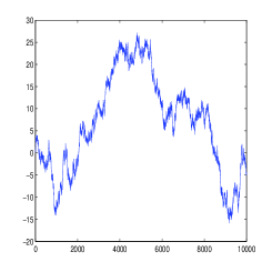
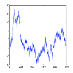
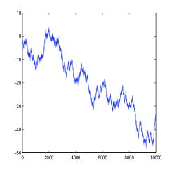
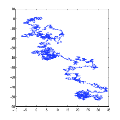
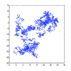
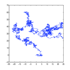
Figure 17: Illustration of a Brownian motion. Upper figures: one–dimensional Brownian motion – three realizations of $x(t)$ as a function of $t$. Lower figures: two–dimensional Brownian motion – three realizations of $\vec{\mbox{\boldmath$r$}}(t)=[x(t),y(t)]$. All realizations start at the origin.

We may visualize each collision on the pollen grain as that of an impulse, because the duration of each collision is extremely short. In other words, the position of the particle $x(t)$ is responding to a sequence of (positive and negative) impulses at random times. Let

$$R_{v}(\tau)=\left<v(t)v(t+\tau)\right>=\left<\dot{x}(t)\dot{x}(t+\tau)\right>$$ (8.2.8)

denote the autocorrelation of the random process $v(t)=\dot{x}(t)$ and let $S_{v}(\omega)={\cal F}\{R_{v}(\tau)\}$ be the power spectral density.

Clearly, by the Langevin equation $\{v(t)\}$ is the response of a linear, time–invariant linear system

$$H(s)=\frac{1}{ms+\gamma}=\frac{1}{m(s+1/\theta)};~{}~{}~{}~{}~{}~{}~{}h(t)=\frac{1}{m}e^{-t/\theta}u(t)$$ (8.2.9)

to the random input process $\{F_{r}(t)\}$. Assuming that the impulse process $\{F_{r}(t)\}$ is white noise, then

$$R_{v}(\tau)=\mbox{const}\cdot h(\tau)*h(-\tau)=\mbox{const}\cdot e^{-|\tau|/\theta}=R_{v}(0)e^{-|\tau|/\theta}=\frac{kT}{m}\cdot e^{-|\tau|/\theta}$$ (8.2.10)

and

$$S_{v}(\omega)=\frac{2kT}{m}\cdot\frac{\omega_{0}}{\omega^{2}+\omega_{0}^{2}},~{}~{}~{}~{}~{}\omega_{0}=\frac{1}{\theta}=\frac{\gamma}{m}$$ (8.2.11)

that is, a Lorentzian spectrum. We see that the relaxation time $\theta$ is indeed a measure of the “memory” of the particle and $\omega_{0}=1/\theta$ plays the role of 3dB cutoff frequency of the spectrum of $\{v(t)\}$. What is the spectral density of the driving input white noise process?

$$S_{F_{r}}(\omega)=\frac{S_{v}(\omega)}{|H(i\omega)|^{2}}=\frac{2kT\omega_{0}}{m(\omega^{2}+\omega_{0}^{2})}\cdot m^{2}(\omega^{2}+\omega_{0}^{2})=2kTm\omega_{0}=2kT\gamma.$$ (8.2.12)

This is a very important result. The spectral density of the white noise is $2kT$ times the dissipative coefficient of the system, $\gamma$. In other words, the dissipative element of the system is ‘responsible’ for the noise. At first glance, it may seem surprising: Why should the intensity of the (external) driving force $F_{r}(t)$ be related to the dissipative coefficient $\gamma$? The answer is that they are related via energy balance considerations, since we are assuming thermal equilibrium. Because the energy waste (dissipation) is proportional to $\gamma$, the energy supply from $F_{r}(t)$ must also be proportional to $\gamma$ in order to balance it.

Example 8.2 – Energy balance for the Brownian particle. The friction force $F_{friction}(t)=-\gamma v(t)$ causes the particle to loose kinetic energy at the rate of

$$P_{loss}=\left<F_{friction}(t)v(t)\right>=-\gamma\left<v^{2}(t)\right>=-\gamma\cdot\frac{kT}{m}=-\frac{kT}{\theta}.$$

On the other hand, the driving force $F_{r}(t)$ injects kinetic energy at the rate of

$$P_{injected} = \left<F_{r}(t)v(t)\right>$$ (8.2.13)

$$= \left<F_{r}(t)\int_{0}^{\infty}\mbox{d}\tau h(\tau)F_{r}(t-\tau)\right>$$ (8.2.14)

$$= 2kT\gamma\int_{0}^{\infty}\mbox{d}\tau h(\tau)\delta(\tau)$$ (8.2.15)

$$= kT\gamma h(0)=\frac{kT\gamma}{m}=\frac{kT}{\theta},$$ (8.2.16)

which exactly balances the loss. Here, we used that fact that $\int_{0}^{\infty}\mbox{d}\tau h(\tau)\delta(\tau)=h(0)/2$ since only “half” of the delta function is “alive” where $h(\tau)>0$. Exercise 8.2: What happens if $\gamma=0$, yet $F_{r}(t)$ has spectral density $N_{0}$? Calculate the rate of kinetic energy increase in two different ways: (i) Show that $\frac{m}{2}\left<v^{2}(t)\right>$ is linear in $t$ and find the constant of proportionality. (ii) calculate $\left<F_{r}(t)v(t)\right>$ for this case.

These principles apply not only to a Brownian particle in a liquid, but to any linear system that obeys a first order stochastic differential equation with a white noise input, provided that the energy equipartition theorem applies. An obvious electrical analogue of this is a simple electric circuit where a resistor $R$ and a capacitor $C$ are connected to one another (see Fig. 18).

Figure 18: An $R$–$C$ circuit.

The thermal noise generated by the resistor (due to the thermal random motion of the colliding free electrons in the conductor with extremely short mean time between collisions), a.k.a. the Johnson–Nyquist noise, is modeled as a current source connected in parallel to the resistor (or as an equivalent voltage source connected in series to the resistor), which generates a white noise current process $I_{r}(t)$. The differential equation pertaining to Kirchoff’s current law is

$$C\dot{V}(t)+\frac{V(t)}{R}=I_{r}(t)$$ (8.2.17)

where $V(t)$ is the voltage across the resistor as well as the parallel capacitor. Now, this is exactly the same differential equation as before, where $I_{r}(t)$ plays the role of the driving force, $V(t)$ is replacing $\dot{x}(t)$, $C$ substitutes $m$, and $1/R$ is the dissipative coefficient instead of $\gamma$. Thus, the spectral density of the current is

$$S_{I_{r}}(\omega)=\frac{2kT}{R}.$$ (8.2.18)

Alternatively, if one adopts the equivalent serial voltage source model then $V_{r}(t)=RI_{r}(t)$ and so

$$S_{V_{r}}(\omega)=\frac{2kT}{R}\cdot R^{2}=2kTR.$$ (8.2.19)

These results are well–knon from elementrary courses on random processes.

Finally, note that here we have something similar the ultraviolet catastrophe: White noise has infinite power, which is unphysical. Once again, this happens because we are working in the classical regime and we have not addressed quantum effects pertaining to very high frequencies ($\hbar\omega\gg kT$), which similarly as in black–body radiation, cause a sharp (exponential) decay in the spectrum beyond a cutoff frequency of the order of magnitude of $kT/\hbar$ (which is a huge frequency at room temperature). We will get back to this later on in Subsection 8.5.

8.3 Diffusion and the Fokker–Planck Equation

In this subsection, we consider the temporal evolution of the probability density function of $x(t)$ (and not only its second order statistics, as in the previous subsection), under quite general conditions.

The first successful treatment of Brownian motion was due to Einstein, who as mentioned earlier, reduced the problem to one of diffusion. It might be speculated that his motivation was that the diffusion equation is the simplest differential equation in mathematical physics, which is asymmetric in time: Since it includes a first order derivative w.r.t. $t$, replacing $t$ by $-t$ changes the equation. Because the Brownian motion is irreversible, it was important to include this feature in the analysis. Einstein’s argument can be summarized as follows: Assume that each particle moves independently of all other particles. The relaxation time is small compared to the observation time, but is long enough for the motions of a particle in two consecutive intervals of $\theta$ to be independent.

Let the number of suspended grains be $N$ and let the $x$ coordinate change by $\Delta$ in one relaxation time. $\Delta$ is a random variable, symmetrically distributed around $\Delta=0$. The number of particles $\mbox{d}N$ which are displaced by more than $\Delta$ but less than $\Delta+\mbox{d}\Delta$ is

$$\mbox{d}N=Np(\Delta)\mbox{d}\Delta$$ (8.3.1)

where $p(\Delta)$ is the pdf of $\Delta$. Since only small displacements are likely to occur, $p(\Delta)$ is sharply peaked at the origin. Let $\rho(x,t)$ denote the density of particles at position $x$, at time $t$. The number of particles in the interval $[x,x+\mbox{d}x]$ at time $t+\delta$ ($\delta$ small) is

$$\rho(x,t+\delta)\mbox{d}x=\mbox{d}x\int_{-\infty}^{+\infty}\rho(x-\Delta,t)p(\Delta)\mbox{d}\Delta$$ (8.3.2)

This equation simply tells that the probability of finding the particle around $x$ at time $t+\delta$ is made of contributions of finding it in $x-\Delta$ at time $t$, and then moving by $\Delta$ within duration $\delta$ to arrive at $x$ at time $t+\delta$. Here we assumed independence between the location $x-\Delta$ at time $t$ and the probability distribution of the displacement $\Delta$, as $p(\Delta)$ is independent of $x-\Delta$. Since $\theta$ is small, we take the liberty to use the Taylor series expansion

$$\rho(x,t+\delta)\approx\rho(x,t)+\delta\cdot\frac{\partial\rho(x,t)}{\partial t}$$ (8.3.3)

Also, for small $\Delta$, we approximate $\rho(x-\Delta,t)$, this time to the second order:

$$\rho(x-\Delta,t)\approx\rho(x,t)-\Delta\cdot\frac{\partial\rho(x,t)}{\partial x}+\frac{\Delta^{2}}{2}\cdot\frac{\partial^{2}\rho(x,t)}{\partial x^{2}}$$ (8.3.4)

Putting these in eq. (8.3.2), we get

$$\rho(x,t)+\delta\cdot\frac{\partial\rho(x,t)}{\partial t} = \rho(x,t)\int_{-\infty}^{+\infty}p(\Delta)\mbox{d}\Delta-\frac{\partial\rho(x,t)}{\partial x}\int_{-\infty}^{+\infty}\Delta p(\Delta)\mbox{d}\Delta+$$ (8.3.5)

$$\frac{1}{2}\cdot\frac{\partial^{2}\rho(x,t)}{\partial x^{2}}\int_{-\infty}^{+\infty}\Delta^{2}p(\Delta)\mbox{d}\Delta$$

or

$$\frac{\partial\rho(x,t)}{\partial t}=\frac{1}{2\delta}\cdot\frac{\partial^{2}\rho(x,t)}{\partial x^{2}}\int_{-\infty}^{+\infty}\Delta^{2}p(\Delta)\mbox{d}\Delta$$ (8.3.6)

which is the diffusion equation

$$\frac{\partial\rho(x,t)}{\partial t}=D\cdot\frac{\partial^{2}\rho(x,t)}{\partial x^{2}}$$ (8.3.7)

with the diffusion coefficient being

$$D=\lim_{\delta\to 0}\frac{\left<\Delta^{2}\right>}{2\delta}=\lim_{\delta\to 0}\frac{\left<[x(t+\delta)-x(t)]^{2}\right>}{2\delta}.$$ (8.3.8)

To solve the diffusion equation, define $\varrho(\kappa,t)$ as the Fourier transform of $\rho(x,t)$ w.r.t. the variable $x$, i.e.,

$$\varrho(\kappa,t)=\int_{-\infty}^{+\infty}\mbox{d}x\cdot e^{-i\kappa x}\rho(x,t).$$ (8.3.9)

Then, the diffusion equation becomes an ordinary differential equation w.r.t. $t$:

$$\frac{\varrho(\kappa,t)}{\partial t}=D(i\kappa)^{2}\varrho(\kappa,t)\equiv-D\kappa^{2}\varrho(\kappa,t)$$ (8.3.10)

whose solution is easily found to be

$$\varrho(\kappa,t)=C(\kappa)e^{-D\kappa^{2}t}.$$ (8.3.11)

Assuming that the particle is initially located at the origin, i.e., $\rho(x,0)=\delta(x)$, this means that the initial condition is $C(\kappa)=\varrho(\kappa,0)=1$ for all $\kappa$, and so

$$\varrho(\kappa,t)=e^{-D\kappa^{2}t}.$$ (8.3.12)

The density $\rho(x,t)$ is now obtained by the inverse Fourier transform, which is

$$\rho(x,t)=\frac{e^{-x^{2}/(4Dt)}}{\sqrt{4\pi Dt}},$$ (8.3.13)

and so $x(t)$ is zero–mean Gaussian with variance $\left<x^{2}(t)\right>=2Dt$. Of course, any other initial location $x_{0}$ would yield a Gaussian with the same variance $2Dt$, but the mean would be $x_{0}$. Comparing the variance $2Dt$ with eq. (8.2.7), we have

$$D=\frac{kT}{\gamma}$$ (8.3.14)

which is known as the Einstein relation, widely used in semiconductor physics.

The analysis thus far assumed that $\left<\Delta\right>=0$, namely, there is no drift to either the left or the right direction. We next drop this assumption. In this case, the diffusion equation generalizes to

$$\frac{\partial\rho(x,t)}{\partial t}=-v\cdot\frac{\partial\rho(x,t)}{\partial x}+D\cdot\frac{\partial^{2}\rho(x,t)}{\partial x^{2}}$$ (8.3.15)

where

$$v=\lim_{\delta\to 0}\frac{\left<\Delta\right>}{\delta}=\lim_{\delta\to 0}\frac{\left<x(t+\delta)-x(t)\right>}{\delta}=\frac{\mbox{d}}{\mbox{d}t}\left<\dot{x}(t)\right>$$ (8.3.16)

has the obvious meaning of the average velocity. Eq. (8.3.15) is well known as the Fokker–Planck equation. The diffusion equation and the Fokker–Planck equation are very central in physics. As mentioned already in Chapter 2, they are fundamental in semiconductor physics, as they describe processes of propagation of concentrations of electrons and holes in semiconductor materials.

Exercise 8.3. Solve the Fokker–Planck equation and show that the solution is $\rho(x,t)={\cal N}(vt,2Dt)$. Explain the intuition.

It is possible to further extend the Fokker–Planck equation so as to allow the pdf of $\Delta$ to be location–dependent, that is, $p(\Delta)$ would be replaced by $p_{x}(\Delta)$, but the important point to retain is that given the present location $x(t)=x$, $\Delta$ would be independent of the earlier history of $\{x(t^{\prime}),t^{\prime}<t\}$, which is to say that $\{x(t)\}$ should be a Markov process. Consider then a general continuous–time Markov process defined by the transition probability density function $W_{\delta}(x^{\prime}|x)$, which denotes the pdf of $x(t+\delta)$ at $x^{\prime}$ given that $x(t)=x$. A straightforward extension of the earlier derivation would lead to the following more general form

$$\frac{\partial\rho(x,t)}{\partial t}=-\frac{\partial}{\partial x}[v(x)\rho(x,t)]+\frac{\partial^{2}}{\partial x^{2}}[D(x)\rho(x,t)],$$ (8.3.17)

where

$$v(x)=\lim_{\delta\to 0}\frac{1}{\delta}\int_{-\infty}^{+\infty}(x^{\prime}-x)W_{\delta}(x^{\prime}|x)\mbox{d}x^{\prime}=\mbox{\boldmath$E$}[\dot{x}(t)|x(t)=x].$$ (8.3.18)

is the local average velocity and

$$D(x)=\lim_{\delta\to 0}\frac{1}{2\delta}\int_{-\infty}^{+\infty}(x^{\prime}-x)^{2}W_{\delta}(x^{\prime}|x)\mbox{d}x^{\prime}=\lim_{\delta\to 0}\frac{1}{2\delta}\mbox{\boldmath$E$}\{[x(t+\delta)-x(t)]^{2}|x(t)=x\}$$ (8.3.19)

is the local diffusion coefficient.

Example 8.3. Consider the stochastic differential equation

$$\dot{x}(t)=-ax(t)+n(t),$$

where $n(t)$ is Gaussian white noise with spectral density $N_{0}/2$. From the solution of this differential equation, it is easy to see that

$$x(t+\delta)=x(t)e^{-a\delta}+e^{-a(t+\delta)}\int_{t}^{t+\delta}\mbox{d}\tau n(\tau)e^{a\tau}.$$

This relation, between $x(t)$ and $x(t+\delta)$, can be used to derive the first and the second moments of $[x(t+\delta)-x(t)]$ for small $\delta$, and to find that $v(x)=-ax$ and $D(x)=N_{0}/4$ (Exercise 8.5: Show this). Thus, the Fokker–Planck equation, in this example, reads

$$\frac{\partial\rho(x,t)}{\partial t}=a\cdot\frac{\partial}{\partial x}[x\cdot\rho(x,t)]+\frac{N_{0}}{4}\cdot\frac{\partial^{2}\rho(x,t)}{\partial x^{2}}.$$

It is easy to check that the r.h.s. vanishes for $\rho(x,t)\propto e^{-2ax^{2}/N_{0}}$ (independent of $t$), which means that in equilibrium, $x(t)$ is Gaussian with zero mean and variance $N_{0}/4a$. This is in agreement with the fact that, as $x(t)$ is the response of the linear system $H(s)=1/(s+a)$ (or in the time domain, $h(t)=e^{-at}u(t)$) to $n(t)$, its variance is indeed (as we know from “Random Signals”):

$$\frac{N_{0}}{2}\int_{0}^{\infty}h^{2}(t)\mbox{d}t=\frac{N_{0}}{2}\int_{0}^{\infty}e^{-2at}\mbox{d}t=\frac{N_{0}}{4a}.$$

Note that if $x(t)$ is the voltage across the capacitor in a simple $R$–$C$ network, then $a=1/RC$, and since ${\cal E}(x)=Cx^{2}/2$, then in equilibrium we have the Boltzmann weight $\rho(x)\propto\exp(-Cx^{2}/2kT)$, which is again, a zero–mean Gaussian. Comparing the exponents, we immediately obtain $N_{0}/2=2kT/RC^{2}$. Exercise 8.6: Find the solution $\rho(x,t)$ for all $x$ and $t$ subject to the initial condition $\rho(x,0)=\delta(x)$. $\Box$

A slightly different representation of the Fokker–Planck equation is the following:

$$\frac{\partial\rho(x,t)}{\partial t}=-\frac{\partial}{\partial x}\left\{v(x)\rho(x,t)-\frac{\partial}{\partial x}[D(x)\rho(x,t)]\right\},$$ (8.3.20)

Now, $v(x)\rho(x,t)$ has the obvious interpretation of the drift current density $J_{\mbox{\tiny drift}}(x,t)$ of a ‘mass’ whose density is $\rho(x,t)$ (in this case, it is a probability mass), whereas

$$J_{\mbox{\tiny diffusion}}(x,t)=-\frac{\partial}{\partial x}[D(x)\rho(x,t)]$$

is the diffusion current density. Thus,

$$\frac{\partial\rho(x,t)}{\partial t}=-\frac{\partial J_{\mbox{\tiny total}}(x,t)}{\partial x}$$ (8.3.21)

where

$$J_{\mbox{\tiny total}}(x,t)=J_{\mbox{\tiny drift}}(x,t)+J_{\mbox{\tiny diffusion}}(x,t).$$

Eq. (8.3.21) is the equation of continuity, which we saw in Chapter 2. In steady state, when $\rho(x,t)$ is time–invariant, the total current may vanish. The drift current and the diffusion current balance one another, or at least the net current is homogenous (independent of $x$), so no mass accumulates anywhere.

Comment. It is interesting to relate the diffusion constant $D$ to the mobility of the electrons in the context of electric conductivity. The mobility $\mu$ is defined according to $v=\mu E$, where $E$ is the electric field. According to Fick’s law, the current density is proportional to the negative gradient of the concentration, and $D$ is defined as the constant of proportionality, i.e., $J_{\mbox{\tiny electrons}}=-D\partial\rho/\partial x$ or $J=-Dq_{e}\partial\rho/\partial x$. If one sets up a field $E$ in an open circuit, the diffusion current cancels the drift current, that is

$$J=\rho q_{e}\mu E-Dq_{e}\frac{\partial\rho}{\partial x}=0$$ (8.3.22)

which would give $\rho(x)\propto e^{\mu Ex/D}$. On the other hand, under thermal equilibrium, with potential energy $V(x)=-q_{e}Ex$, we also have $\rho(x)\propto e^{-V/kT}=e^{q_{e}Ex/kT}$. Upon comparing the exponents, we readily obtain the Einstein relation $D=kT\mu/q_{e}$. Note that $\mu/q_{e}=v/q_{e}E$ is related to the admittance (the dissipative coefficient) since $v$ is proportional to the current and $E$ is proportional to the voltage.

8.4 The Fluctuation–Dissipation Theorem

We next take another point of view on stochastic dynamics of a physical system: Suppose that a system (not necessarily a single particle as in the previous subsections) is initially in equilibrium of the canonical ensemble, but at a certain time instant, it is subjected to an abrupt, yet small change in a certain parameter that controls it (say, a certain force, like pressure, magnetic field, etc.). Right after this abrupt change in the parameter, the system is, of course, no longer in equilibrium, but it is not far, since the change is assumed small. How fast does the system re–equilibrate and what is its dynamical behavior in the course of the passage to the new equilibrium? Also, since the change was abrupt and not quasi–static, how is energy dissipated? Quite remarkably, it turns out that the answers to both questions are related to the equilibrium fluctuations of the system. Accordingly, the principle that quantifies and characterizes this relationship is called the fluctuation–dissipation theorem and this is the subject of this subsection. We shall also relate it to the derivations of the previous subsection.

Consider a physical system, which in the absence of any applied external field, has an Hamiltonian ${\cal E}(x)$, where here $x$ denotes the microstate, and so, its equilibrium distribution is the Boltzmann distribution with a partition function given by:

$$Z(\beta)=\sum_{x}e^{-\beta{\cal E}(x)}.$$ (8.4.1)

Now, let $w_{x}$ be an observable (a measurable physical quantity that depends on the microstate), which has a conjugate force $F$, so that when $F$ is applied, the change in the Hamiltonian is $\Delta{\cal E}(x)=-Fw_{x}$. Next suppose that the external force is time–varying according to a certain waveform $\{F(t),~{}-\infty<t<\infty\}$. As in the previous subsection, it should be kept in mind that the overall effective force can be thought of as a superposition of two contributions, a deterministic contribution, which is the above mentioned $F(t)$ – the external field that the experimentalist applies on purpose and fully controls, and a random part $F_{r}(t)$, which pertains to interaction with the environment (or the heat bath at temperature $T$). The random component $F_{r}(t)$ is responsible for the randomness of the microstate $x$ and hence also the randomness of the observable. We shall denote the random variable corresponding to the observable at time $t$ by $W(t)$. Thus, $W(t)$ is random variable, which takes values in the set $\{w_{x},~{}x\in{\cal X}\}$, where ${\cal X}$ is the space of microstates. When the external deterministic field is kept fixed ($F(t)\equiv\mbox{const.}$), the system is expected to converge to equilibrium and eventually obey the Boltzmann law. While in the section on Brownian motion, we focused only on the contribution of the random part, $F_{r}(t)$, now let us refer only to the deterministic part, $F(t)$. We will get back to the random part later on.

Let us assume first that $F(t)$ was switched on to a small level $\epsilon$ at time $-\infty$, and then switched off at time $t=0$, in other words, $F(t)=\epsilon U(-t)$, where $U(\cdot)$ is the unit step function (a.k.a. the Heaviside function). We are interested in the behavior of the mean of the observable $W(t)$ at time $t$, which we shall denote by $\left<W(t)\right>$, for $t>0$. Also, $\left<W(\infty)\right>$ will denote the limit of $\left<W(t)\right>$ as $t\to\infty$, namely, the equilibrium mean of the observable in the absence of an external field. Define now the (negative) step response function as

$$\zeta(t)=\lim_{\epsilon\to 0}\frac{\left<W(t)\right>-\left<W(\infty)\right>}{\epsilon}$$ (8.4.2)

and the auto–covariance function pertaining to the final equilibrium as

$$R_{W}(\tau)\stackrel{{\scriptstyle\Delta}}{{=}}\lim_{t\to\infty}\left<W(t)W(t+\tau)\right>-\left<W(\infty)\right>^{2},$$ (8.4.3)

Then, the fluctuation–dissipation theorem (FDT) asserts that

$$R_{W}(\tau)=kT\cdot\zeta(\tau)$$ (8.4.4)

The FDT then relates between the linear transient response of the system to a small excitation (after it has been removed) and the autocovariance of the observable in equilibrium. The transient response, that fades away is the dissipation, whereas the autocovariance is the fluctuation. Normally, $R_{W}(\tau)$ decays for large $\tau$ and so $\left<W(t)\right>$ converges to $\left<W(\infty)\right>$ at the same rate (see Fig. 19).

Figure 19: Illustration of the response of $\left<W(t)\right>$ to a step function at the input force $F(t)=\epsilon U(-t)$. According to the FDT, the response (on top of the asymptotic level $\left<W(\infty)\right>$) is proportional to the equilibrium autocorrelation function $R_{W}(t)$, which in turn may decay either monotonically (solid curve) or in an oscillatory manner (dashed curve).

To prove this result, we proceed as follows: First, we have by definition:

$$\left<W(\infty)\right>=\frac{\sum_{x}w_{x}e^{-\beta{\cal E}(x)}}{\sum_{x}e^{-\beta{\cal E}(x)}}$$ (8.4.5)

Now, for $t<0$, we have

$$P(x)=\frac{e^{-\beta{\cal E}(x)-\beta\Delta{\cal E}(x)}}{\sum_{x}e^{-\beta{\cal E}(x)-\beta\Delta{\cal E}(x)}}.$$ (8.4.6)

Thus, for all negative times, and for $t=0^{-}$ in particular, we have

$$\left<W(0^{-})\right>=\frac{\sum_{x}w_{x}e^{-\beta{\cal E}(x)-\beta\Delta{\cal E}(x)}}{\sum_{x}e^{-\beta{\cal E}(x)-\beta\Delta{\cal E}(x)}}.$$ (8.4.7)

Let $P_{t}(x^{\prime}|x)$ denote the probability that the system would be at state $x^{\prime}$ at time $t$ ($t>0$) given that it was in state $x$ at time $t=0^{-}$. This probability depends on the dynamical properties of the system (in the absence of the perturbing force). Let us define $\left<W(t)\right>_{x}=\sum_{x^{\prime}}w_{x^{\prime}}P_{t}(x^{\prime}|x)$, which is the expectation of $W(t)$ ($t>0$) given that the system was in state $x$ at $t=0^{-}$. Now,

$$\left<W(t)\right> = \frac{\sum_{x}\left<W(t)\right>_{x}e^{-\beta{\cal E}(x)-\beta\Delta{\cal E}(x)}}{\sum_{x}e^{-\beta{\cal E}(x)-\beta\Delta{\cal E}(x)}}$$ (8.4.8)

$$= \frac{\sum_{x}\left<W(t)\right>_{x}e^{-\beta{\cal E}(x)+\beta\epsilon w_{x}}}{\sum_{x}e^{-\beta{\cal E}(x)+\beta\epsilon w_{x}}}$$

and $\left<W(\infty)\right>$ can be seen as a special case of this quantity for $\epsilon=0$ (no perturbation at all). Thus, $\zeta(t)$ is, by definition, nothing but the derivative of $\left<W(t)\right>$ w.r.t. $\epsilon$, computed at $\epsilon=0$. I.e.,

$$\zeta(\tau) = \frac{\partial}{\partial\epsilon}\left[\frac{\sum_{x}\left<W(\tau)\right>_{x}e^{-\beta{\cal E}(x)+\beta\epsilon w_{x}}}{\sum_{x}e^{-\beta{\cal E}(x)+\beta\epsilon w_{x}}}\right]_{\epsilon=0}$$ (8.4.9)

$$= \beta\cdot\frac{\sum_{x}\left<W(\tau)\right>_{x}w_{x}e^{-\beta{\cal E}(x)}}{\sum_{x}e^{-\beta{\cal E}(x)}}-\beta\cdot\frac{\sum_{x}\left<W(\tau)\right>_{x}e^{-\beta{\cal E}(x)}}{\sum_{x}e^{-\beta{\cal E}(x)}}\cdot\frac{\sum_{x}w_{x}e^{-\beta{\cal E}(x)}}{\sum_{x}e^{-\beta{\cal E}(x)}}$$

$$= \beta\left[\lim_{t\to\infty}\left<W(t)W(t+\tau)\right>-\left<W(\infty)\right>^{2}\right]$$

$$= \beta R_{W}(\tau),$$

where we have used the fact that the dynamics of $\{P_{t}(x^{\prime}|x)\}$ preserve the equilibrium distribution.

Exercise 8.7. Extend the FDT to account for a situation where the force $F(t)$ is not conjugate to $W(t)$, but to another physical quantity $V(t)$.

While $\zeta(t)$ is essentially the response of the system to a (negative) step function in $F(t)$, then obviously,

$$h(t)=\left\{\begin{array}[]{cc}0&t<0\\ -\dot{\zeta}(t)&t\geq 0\end{array}\right.=\left\{\begin{array}[]{cc}0&t<0\\ -\beta\dot{R}_{W}(t)&t\geq 0\end{array}\right.$$ (8.4.10)

would be the impulse response. Thus, we can now express the response of $\left<W(t)\right>$ to a general signal $F(t)$ that vanishes for $t>0$ to be

$$\left<W(t)\right>-\left<W(\infty)\right> \approx -\beta\int_{-\infty}^{0}\dot{R}_{W}(t-\tau)F(\tau)\mbox{d}\tau$$ (8.4.11)

$$= -\beta\int_{-\infty}^{0}R_{W}(t-\tau)\dot{F}(\tau)\mbox{d}\tau$$

$$= -\beta R_{W}\otimes\dot{F},$$

where the second passage is from integration by parts and where $\otimes$ denotes convolution. Indeed, in our first example, $\dot{F}(t)=-\epsilon\delta(t)$ and we are back to the result $\left<W(t)\right>-\left<W(\infty)\right>=\beta\epsilon R_{W}(t)$.

It is instructive to look at these relations also in the frequency domain. Applying the one sided Fourier transform on both sides of the relation $h(t)=-\beta\dot{R}_{W}(t)$ and taking the complex conjugate (i.e., multiplying by $e^{i\omega t}$ and integrating over $t>0$), we get

$$H(-i\omega)\equiv\int_{0}^{\infty}h(t)e^{i\omega t}\mbox{d}t=-\beta\int_{0}^{\infty}\dot{R}_{W}(t)e^{i\omega t}\mbox{d}t=\beta i\omega\int_{0}^{\infty}R_{W}(t)e^{i\omega t}\mbox{d}t+\beta R_{W}(0),$$ (8.4.12)

where the last step is due to integration by parts. Upon taking the imaginary parts of both sides, we get:

$$\mbox{Im}\{H(-i\omega)\}=\beta\omega\int_{0}^{\infty}R_{W}(t)\cos(\omega t)\mbox{d}t=\frac{1}{2}\beta\omega S_{W}(\omega),$$ (8.4.13)

where $S_{W}(\omega)$ is the power spectrum of $\{W(t)\}$ in equilibrium, that is, the Fourier transform of $R_{W}(\tau)$. Equivalently, we have:

$$S_{W}(\omega)=2kT\cdot\frac{\mbox{Im}\{H(-i\omega)\}}{\omega}=-2kT\cdot\frac{\mbox{Im}\{H(i\omega)\}}{\omega}$$ (8.4.14)

Example 8.4 An electric circuit. Consider the circuit in Fig. 20. The driving force is the voltage source $V(t)$ and the conjugate variable is $Q(t)$ the of the capacitor. The resistors are considered part of thermal environment. The voltage waveform is $V(t)=\epsilon U(-t)$. At time $t=0^{-}$, the voltage across the capacitor is $\epsilon/2$ and the energy is $\frac{1}{2}C(V_{r}+\frac{\epsilon}{2})^{2}$, whereas for $t\to\infty$, it is $\frac{1}{2}CV_{r}^{2}$, so the difference is $\Delta{\cal E}=\frac{1}{2}CV_{r}\epsilon=\frac{1}{2}Q_{r}\epsilon$, neglecting the $O(\epsilon^{2})$ term. According to the FDT then, $\zeta(t)=\frac{1}{2}\beta R_{Q}(t)$, where the factor of $1/2$ follows the one in $\Delta{\cal E}$. This then gives

$$S_{Q}(\omega)=4kT\cdot\frac{\mbox{Im}\{H(-i\omega)\}}{\omega}.$$ (8.4.15)

In this case,

$$H(i\omega)=\frac{(R\|1/[i\omega C])\cdot C}{R+(R\|1/[i\omega C])}=\frac{C}{2+i\omega RC}$$ (8.4.16)

for which

$$\mbox{Im}\{H(-i\omega)\}=\frac{\omega RC^{2}}{4+(\omega RC)^{2}}$$ (8.4.17)

and finally,

$$S_{Q}(\omega)=\frac{4kTRC^{2}}{4+(\omega RC)^{2}}$$ (8.4.18)

Thus, the thermal noise voltage across the capacitor is $4kTR/[4+(\omega RC)^{2}]$. The same result can be obtained, of course, using the method studied in “Random Signals”:

$$2kT\cdot\mbox{Re}\left\{R\|R\|\frac{1}{i\omega C}\right\}=\frac{4kTR}{4+(\omega RC)^{2}}.$$ (8.4.19)

This concludes Example 8.4. $\Box$

Figure 20: Electric circuit for Example 8.4.

Earlier, we have seen that $\left<W(t)\right>-\left<W(\infty)\right>$ responds to a determinstic (small) waveform $F(t)$ via a linear(ized) system with an impulse response $h(t)$. By the same token, we can think of the random part around the mean, $W(t)-\left<W(\infty)\right>$, as the response of the same system to a random input $F_{r}(t)$ (thus, the total response is the superposition). If we wish to think of our physical system in equilibrium as a linear(ized) system with input $F_{r}(t)$ and output $W(t)$, then what would should the spectrum of the input process $\{F_{r}(t)\}$ be in order to comply with the last result? Denoting by $S_{F_{r}}(\omega)$ the spectrum of the input process, we know from “Random Signals” that

$$S_{W}(\omega)=S_{F_{r}}(\omega)\cdot|H(i\omega)|^{2}$$ (8.4.20)

and so comparing with (8.4.14), we have

$$S_{F_{r}}(\omega)=2kT\cdot\frac{\mbox{Im}\{H(-i\omega)\}}{\omega\cdot|H(i\omega)|^{2}}.$$ (8.4.21)

This extends our earlier result concerning the spectrum of the driving white noise in case the Brownian particle, where we obtained a spectral density of $2kT\gamma$.

Example 8.5 – Second order linear system. For a second order linear system (e.g., a damped harmonic oscillator),

$$m\ddot{W}(t)+\gamma\dot{W}(t)+KW(t)=F_{r}(t)$$ (8.4.22)

the force $F_{r}(t)$ is indeed conjugate to the variable $W(t)$, which is the location, as required by the FDT. Here, we have

$$H(i\omega)=\frac{1}{m(i\omega)^{2}+\gamma i\omega+K}=\frac{1}{K-m\omega^{2}+\gamma i\omega}.$$ (8.4.23)

In this case,

$$\mbox{Im}\{H(-i\omega)\}=\frac{\gamma\omega}{(K-m\omega^{2})^{2}+\gamma^{2}\omega^{2}}=\gamma\omega|H(i\omega)|^{2}$$ (8.4.24)

and so, we readily obtain

$$S_{F_{r}}(\omega)=2kT\gamma,$$ (8.4.25)

recovering the principle that the spectral density of the noise process is $2kT$ times the dissipative coefficient $\gamma$ of the system, which is responsible to the irreversible component. The difference between this and the earlier derivation is that earlier, we assumed in advance that the input noise process is white and we only computed its spectral level, whereas now, we have actually shown that at least for a second order linear system like this, it must be white noise (as far as the classical approximation holds).$\Box$

From eq. (8.4.21), we see that the thermal interaction with the environment, when referred to the input of the system, has a spectral density of the form that we can calculate. In general, it does not necessarily have to be a flat spectrum. Consider for example, an arbitrary electric network consisting of one voltage source (in the role of $F(t)$) and a bunch of resistors and capacitors. Suppose that our observable $W(t)$ is the voltage across one of the capacitors. Then, there is a certain transfer function $H(i\omega)$ from the voltage source to $W(t)$. The thermal noise process is contributed by all resistors by considering equivalent noise sources (parallel current sources or serial voltage sources) attached to each resistor. However, in order to refer the contribution of these noise sources to the input $F(t)$, we must calculate equivalent noise sources which are in series with the given voltage source $F(t)$. These equivalent noise sources will no longer generate white noise processes, in general. For example, in the circuit of Fig. 20, if an extra capacitor $C$ would be connected in series to one of the resistors, then, the contribution of the right resistor referred to the left one is not white noise.

8.5 Johnson–Nyquist Noise in the Quantum–Mechanical Regime

As promised at the end of Subsection 8.3, we now return to the problematics of the formula $S_{V_{r}}(\omega)=2kTR$ when it comes to very high frequencies, namely, the electrical analogue to the ultraviolet catastrophe. At very high frequencies, we are talking about very short waves, much shorter than the physical sizes of the electric circuit.

The remedy to the unreasonable classical results in the high frequency range, is to view the motion of electrons in a resistor as an instance of black–body radiation, but instead of the three–dimensional case that we studied earlier, this time, we are talking about the one–dimensional case. The difference is mainly the calculation of the density of states. Consider a long transmission line with characteristic impedance $R$ of length $L$, terminating at both ends by resistances $R$ (see Fig. 21), so that the impedances are matched at both ends. Then any voltage wave propagating along the transmission line is fully absorbed by the terminating resistor without reflection.

Figure 21: Transmission line of length $L$, terminated by resistances $R$ at both ends.

The system resides in thermal equilibrium at temperature $T$. The resistor then can be thought of as a black–body radiator in one dimension. A voltage wave of the form $V(x,t)=V_{0}\exp[i(\kappa x-\omega t)]$ propagates along the transmission line with velocity $v=\omega/\kappa$, which depends on the capacitance and the inductance of the transmission line per unit length. To count the possible modes, let us impose the periodic boundary condition $V(0,t)=V(L,t)$. Then $\kappa L=2\pi n$ for any positive integer $n$. Thus, there are $\Delta n=\Delta\kappa/2\pi$ such modes per unit length in the frequency range between $\omega=v\kappa$ and $\omega+\Delta\omega=v(\kappa+\Delta\kappa)$. The mean energy of such a mode is given by

$$\epsilon(\omega)=\frac{\hbar\omega}{e^{\hbar\omega/kT}-1}.$$ (8.5.1)

Since there are $\Delta n=\Delta\omega/(2\pi v)$ propagating modes per unit length in this frequency range, the mean energy per unit time (i.e., the power) incident upon a resistor in this frequency range is

$$P=\frac{L}{L/v}\cdot\frac{\Delta\omega}{2\pi v}\cdot\epsilon(\omega)=\frac{1}{2\pi}\cdot\frac{\hbar\omega\Delta\omega}{e^{\hbar\omega/kT}-1},$$ (8.5.2)

where $L/v$ at the denominator is the travel time of the wave along the transmission line. This is the radiation power absorbed by the resistor, which must be equal to the power emitted by the resistor in this frequency range. Let the thermal voltage generated by the resistor in the frequency range $[\omega,\omega+\Delta\omega]$ be denoted by $V_{r}(t)[\omega,\omega+\Delta\omega]$. This voltage sets up a current of $V_{r}(t)[\omega,\omega+\Delta\omega]/2R$ and hence an average power of $\left<V_{r}^{2}(t)[\omega,\omega+\Delta\omega]\right>/4R$. Thus, the balance between the absorbed and the emitted power gives

$$\frac{\left<V_{r}^{2}(t)[\omega,\omega+\Delta\omega]\right>}{4R}=\frac{1}{2\pi}\cdot\frac{\hbar\omega\cdot\Delta\omega}{e^{\hbar\omega/kT}-1},$$ (8.5.3)

which is

$$\frac{\left<V_{r}^{2}(t)[\omega,\omega+\Delta\omega]\right>}{\Delta\omega}=\frac{4R}{2\pi}\cdot\frac{\hbar\omega}{e^{\hbar\omega/kT}-1}$$ (8.5.4)

or

$$\frac{\left<V_{r}^{2}(t)[f,f+\Delta f]\right>}{\Delta f}=4R\cdot\frac{\hbar\omega}{e^{\hbar\omega/kT}-1}$$ (8.5.5)

Taking the limit $\Delta f\to 0$, the left–hand side becomes the one–sided spectral density of the thermal noise, and so the two–sided spectral density is

$$S_{V_{r}}(\omega)=2R\cdot\frac{\hbar\omega}{e^{\hbar\omega/kT}-1}.$$ (8.5.6)

We see then that when quantum–mechanical considerations are incorporated, the noise spectrum is no longer strictly flat. As long as $\hbar\omega\ll kT$, the denominator is very well approximated by $\hbar\omega/kT$, and so we recover the formula $2kTR$, but for frequencies of the order of magnitude of $\omega_{c}\stackrel{{\scriptstyle\Delta}}{{=}}kT/\hbar$, the spectrum falls off exponentially rapidly. So the quantum–mechanical correction is to replace

$$kT~{}\Longrightarrow~{}\frac{\hbar\omega}{e^{\hbar\omega/kT}-1}.$$ (8.5.7)

At room temperature ($T=300^{o}K$), the cutoff frequency is $f_{c}=\omega_{c}/2\pi\approx 6.2\mbox{THz}$, so the spectrum can be safely considered $2kTR$ flat over any frequency range of practical interest from the engineering perspective.

What is the total RMS noise voltage generated by a resistor $R$ at temperature $T$? The total mean square noise voltage is

$$\left<V_{r}^{2}(t)\right> = 4R\int_{0}^{\infty}\frac{hf\mbox{d}f}{e^{hf/kT}-1}$$ (8.5.8)

$$= \frac{4R(kT)^{2}}{h}\int_{0}^{\infty}\frac{x\mbox{d}x}{e^{x}-1}$$

$$= \frac{4R(kT)^{2}}{h}\int_{0}^{\infty}\frac{xe^{-x}\mbox{d}x}{1-e^{-x}}$$

$$= \frac{4R(kT)^{2}}{h}\sum_{n=1}^{\infty}\int_{0}^{\infty}xe^{-nx}\mbox{d}x$$

$$= \frac{4R(kT)^{2}}{h}\sum_{n=1}^{\infty}\frac{1}{n^{2}}$$

$$= \frac{2R(\pi kT)^{2}}{3h},$$

which is quadratic in $T$ since both the (low frequency) spectral density and the effective bandwidth are linear in $T$. The RMS is then

$$V_{RMS}=\sqrt{\left<V_{r}^{2}(t)\right>}=\sqrt{\frac{2R}{3h}}\cdot\pi kT,$$ (8.5.9)

namely, proportional to temperature and to the square root of the resistance. To get an idea of the order of magnitude, a resistor of $100\Omega$ at temperature $T=300^{o}$K generates an RMS thermal noise of about $4$mV. The equivalent noise bandwidth is

$$B_{eq}=\frac{2R(\pi kT)^{2}/3h}{2kTR}=\frac{\pi^{2}kT}{3h}=\frac{\pi^{2}}{3}\cdot f_{c}.$$ (8.5.10)

Exercise 8.9: Derive an expression for the autocorrelation function of the Johnson–Nyquist noise in the quantum mechnical regime.

8.6 Other Noise Sources

In addition to thermal noise, that we have discussed thus far, there are other physical mechanisms that generate noise in Nature in general, and in electronic circuits, in particular. We will not cover them in great depth here, but only provide short descriptions.

Flicker noise, also known as $1/f$ noise, is a random process with a spectrum that falls off steadily into the higher frequencies, with a pink spectrum. It occurs in almost all electronic devices, and results from a variety of effects, though always related to a direct current. According to the underlying theory, there are fluctuations in the conductivity due to the superposition of many independent thermal processes of alternate excitation and relaxation of certain defects (e.g., dopant atoms or vacant lattice sites). This means that every once in a while, a certain lattice site or a dopant atom gets excited and it moves into a state of higher energy for some time, and then it relaxes back to the lower energy state until the next excitation. Each one of these excitation/relaxation processes can be modeled as a random telegraph signal with a different time constant $\theta$ (due to different physical/geometric characteristics) and hence contributes a Lorentzian spectrum parametrized by $\theta$. The superposition of these processes, whose spectrum is given by the integral of the Lorentzian function over a range of values of $\theta$ (with a certain weight), gives rise to the $1/f$ behavior over a wide range of frequencies. To see this more concretely in the mathematical language, a random telegraph signal $X(t)$ is given by $X(t)=(-1)^{N(t)}$, where $N(t)$ is a Poisson process of rate $\lambda$. It is a binary signal where the level $+1$ can symbolize excitation and the level $-1$ designates relaxation. Here the dwell times between jumps are exponentially distributed. The autocorrelation function is given by

$$\left<X(t)X(t+\tau)\right> = \left<(-1)^{N(t)+N(t+\tau)}\right>$$ (8.6.1)

$$= \left<(-1)^{N(t+\tau)-N(t)}\right>$$

$$= \left<(-1)^{N(\tau)}\right>$$

$$= e^{-\lambda\tau}\sum_{k=0}^{\infty}\frac{(\lambda\tau)^{k}}{k!}\cdot(-1)^{k}$$

$$= e^{-\lambda\tau}\sum_{k=0}^{\infty}\frac{(-\lambda\tau)^{k}}{k!}$$

$$= e^{-2\lambda\tau}$$

and so the spectrum is Lorentzian:

$$S_{X}(\omega)={\cal F}\{e^{-2\lambda|\tau|}\}=\frac{4\lambda}{\omega^{2}+4\lambda^{2}}=\frac{2\theta}{1+(\omega\theta)^{2}},$$ (8.6.2)

where the time constant is $\theta=1/2\lambda$ and the cutoff frequency is $\omega_{c}=2\lambda$. Now, calculating the integral

$$\int_{\theta_{\min}}^{\theta_{\max}}\mbox{d}\theta\cdot g(\theta)\cdot\frac{2\theta}{1+(\omega\theta)^{2}}$$

with $g(\theta)=1/\theta$, yields a composite spectrum that is proportional to

$$\frac{1}{\omega}\tan^{-1}(\omega\theta_{\max})-\frac{1}{\omega}\tan^{-1}(\omega\theta_{\min}).$$

For $\omega\ll 1/\theta_{\max}$, using the approximation $\tan^{-1}(x)\approx x$ ($|x|\ll 1$), this is approximately a constant. For $\omega\gg 1/\theta_{\min}$, using the approximation $\tan^{-1}(x)\approx\frac{\pi}{2}-\frac{1}{x}$ ($|x|\gg 1$), this is approximately proportional to $1/\omega^{2}$. In between, in the range $1/\theta_{\max}\ll\omega\ll 1/\theta_{\min}$ (assuming that $1/\theta_{\max}\ll 1/\theta_{\min}$), the behavior is accordiong to

$$\frac{1}{\omega}\left(\frac{\pi}{2}-\frac{1}{\omega\theta_{\max}}\right)-\theta_{\min}=\frac{1}{\omega}\left(\frac{\pi}{2}-\frac{1}{\omega\theta_{\max}}-\omega\theta_{\min}\right)\approx\frac{\pi}{2\omega},$$

which is the $1/f$ behavior in this wide range of frequencies. There are several theories why $g(\theta)$ should be inversely proportional to $\theta$, but the truth is that they are not perfect, and the issue of $1/f$ noise is not yet perfectly (and universally) understood.

Shot noise in electronic devices consists of unavoidable random statistical fluctuations of the electric current in an electrical conductor. Random fluctuations are inherent when current flows, as the current is a flow of discrete charges (electrons). The the derivation of the spectrum of shot noise is normally studied in courses on random procsses.

Burst noise consists of sudden step–like transitions between two or more levels (non-Gaussian), as high as several hundred microvolts, at random and unpredictable times. Each shift in offset voltage or current lasts for several milliseconds, and the intervals between pulses tend to be in the audio range (less than 100 Hz), leading to the term popcorn noise for the popping or crackling sounds it produces in audio circuits.

Avalanche noise is the noise produced when a junction diode is operated at the onset of avalanche breakdown, a semiconductor junction phenomenon in which carriers in a high voltage gradient develop sufficient energy to dislodge additional carriers through physical impact, creating ragged current flows.

9 A Brief Touch on Information Theory^∗

9.1 Introduction – What is Information Theory About?

Our last topic in this course is about a very brief and concise description on the relation between statistical physics and information theory, a research field pioneered by Claude Elwood Shannon (1917–2001), whose seminal paper “A Mathematical Theory of Communications” (1948) has established the landmark of this field.

In a nutshell, information theory is a science that focuses on the fundamental limits, on the one hand, the achievable performance, on the other hand, concerning various information processing tasks, including most notably:

1. Data compression (lossless/lossy).

2. Error correction coding (coding for protection against errors due to channel noise.

3. Encryption.

There are also additional tasks of information processing that are considered to belong under the umbrella of information theory, like: signal detection, estimation (parameter estimation, filtering/smoothing, prediction), information embedding, process simulation, extraction of random bits, information relaying, and more.

Core information theory, which is called Shannon theory in the jargon of the professionals, is about coding theorems. It is associated with the development of computable formulas that characterize the best performance that can possibly be achieved in these information processing tasks under some (usually simple) assumptions on the probabilistic models that govern the data, the channel noise, the side information, the jammers if applicable, etc. While in most cases, this theory does not suggest constructive communication systems, it certainly provides insights concerning the features that an optimal (or nearly optimal) communication system must have. Shannon theory serves, first and foremost, as the theoretical basis for modern digital communication engineering. That being said, much of the modern research activity in information theory evolves, not only around Shannon theory, but also on the never-ending efforts to develop methodologies (mostly, specific code structures and algorithms) for designing very efficient communication systems, which hopefully come close to the bounds and the fundamental performance limits.

But the scope of information theory it is not limited merely to communication engineering: it plays a role also in computer science, and many other disciplines, one of them is thermodynamics and statistical mechanics, which is the focus of these remaining lectures. Often, information–theoretic problems are well approached from a statistical–mechanical point of view. We will taste this very briefly in two examples of problems.

In the framework of this course, we will not delve into information theory too deeply, but our purpose would be just to touch upon the interface of these two fields.

9.2 Entropy in Info Theory and in Thermo & Statistical Physics

Perhaps the first relation that crosses one’s mind is that in both fields there is a fundamental notion of entropy. Actually, in information theory, the term entropy was coined in the footsteps of the thermodynamic/statistical–mechanical entropy. Along this course, we have seen already three (seemingly) different forms of the entropy: The first is the thermodynamic entropy defined, in its differential form as

$$\delta S=\delta Q/T,$$ (9.2.1)

which was first introduced by Clausius in 1850. The second is the statistical entropy

$$S=k\ln\Omega,$$ (9.2.2)

which was defined by Boltzmann in 1872. The third is yet another formula for the entropy – the Gibbs formula for the entropy of the canonical ensemble:

$$S=-k\sum_{x}P(x)\ln P(x)=-k\left<\ln P(x)\right>,$$ (9.2.3)

which we encountered in Chapter 3.

It is virtually impossible to miss the functional resemblance between the last form above and the information–theoretic entropy, a.k.a. the Shannon entropy, which is simply

$$H=-\sum_{x}P(x)\log_{2}P(x)$$ (9.2.4)

namely, the same expression as above exactly, just without the factor $k$ and with the basis of the logarithm being 2 rather than $e$. So they simply differ by an immaterial constant factor. Indeed, this clear analogy was recognized already by Shannon and von Neumann. The well–known anecdote on this tells that von Neumann advised Shannon to adopt this term because it would provide him with “… a great edge in debates because nobody really knows what entropy is anyway.”

What is the information–theoretic meaning of entropy? It turns out that it has many information–theoretic meanings, but the most fundamental one concerns optimum compressibility of data. Suppose that we have a bunch of i.i.d. random variables, $x_{1},x_{2},\ldots,x_{N}$, taking values in a discrete set, say, the components of the microstate in a quantum system of non–interacting particles, and we want to represent the microstate information digitally (in bits) as compactly as possible, without losing any information – in other words, we require the ability to fully reconstruct the data from the compressed binary representation. How short can this binary representation be?

Let us look at the following example. Suppose that each $x_{i}$ takes values in the set $\{A,B,C,D\}$, independently with probabilities

$$P(A)=1/2;~{}~{}~{}~{}P(B)=1/4;~{}~{}~{}P(C)=1/8;~{}~{}~{}P(D)=1/8.$$

Clearly, when translating the letters into bits, the naive approach would be to say the following: we have 4 letters, so it takes 2 bits to distinguish between them, by mapping, say lexicographically, as follows:

$$A\to 00;~{}~{}~{}~{}B\to 01;~{}~{}~{}C\to 10;~{}~{}~{}D\to 11.$$

This would mean representing the list of $x$’s using 2 bits per–symbol. Very simple. But is this the best thing one can do?

It turns out that the answer is negative. Intuitively, if we can assign variable–length codewords to the various letters, using shorter codewords for more probably symbols and longer codewords for the less frequent ones, we might be able to gain something. In our example, $A$ is most probable, while $C$ and $D$ are the least probable, so how about the following solution:

$$A\to 0;~{}~{}~{}~{}B\to 10;~{}~{}~{}C\to 110;~{}~{}~{}D\to 111.$$

Now the average number of bits per symbol is:

$$\frac{1}{2}\cdot 1+\frac{1}{4}\cdot 2+\frac{1}{8}\cdot 3+\frac{1}{8}\cdot 3=1.75.$$

We have improved the average bit rate by 12.5%. Splendid. Is this now the best one can do or can we improve even further?

It turns out that this time, the answer is affirmative. Note that in this solution, each letter has a probability of the form $2^{-\ell}$ ($\ell$ – positive integer) and the length of the assigned codeword is exactly $\ell$ (for $A$, $\ell=1$, for $B$ – $\ell=2$, and for $C$ and $D$, $\ell=3$). In other words, the length of the codeword for each letter is the negative logarithm of its probability, so the average number of bits per symbol is $\sum_{x\in\{A,B,C,D\}}P(x)[-\log_{2}P(x)]$, which is exactly the entropy $H$ of the information source. One of the basic coding theorems of information theory tells us that we cannot compress to any coding rate below the entropy and still expect to be able to reconstruct the $x$’s perfectly. But why is this true?

We will not get into a rigorous proof of this statement, but we will make an attempt to give a statistical–mechanical insight into it. Consider the microstate $\mbox{\boldmath$x$}=(x_{1},\ldots,x_{N})$ and let us think of the probability function

$$P(x_{1},\ldots,x_{N})=\prod_{i=1}^{N}P(x_{i})=\exp\left\{-(\ln 2)\sum_{i=1}^{N}\log_{2}[1/P(x_{i})]\right\}$$ (9.2.5)

as an instance of the canonical ensemble at inverse temperature $\beta=\ln 2$, where Hamiltonian is additive, namely, ${\cal E}(x_{1},\ldots,x_{N})=\sum_{i=1}^{N}\epsilon(x_{i})$, with $\epsilon(x_{i})=-\log_{2}P(x_{i})$. Obviously, $Z(\beta)=Z(\ln 2)=1$, so the free energy is exactly zero here. Now, by the weak law of large numbers, for most realizations of the microstate $x$,

$$\frac{1}{N}\sum_{i=1}^{N}\epsilon(x_{i})\approx\left<\epsilon(x_{i})\right>=\left<-\log_{2}P(x_{i})\right>=H,$$ (9.2.6)

so the average ‘internal energy’ is $NH$. It is safe to consider instead the corresponding microcanonical ensemble, which is equivalent as far as macroscopic averages go. In the microcanonical ensemble, we would then have:

$$\frac{1}{N}\sum_{i=1}^{N}\epsilon(x_{i})=H$$ (9.2.7)

for every realization of $x$. How many bits would it take us to represent $x$ in this microcanonical ensemble? Since all $x$’s are equiprobable in the microcanonical ensemble, we assign to all $x$’s binary codewords of the same length, call it $L$. In order to have a one–to–one mapping between the set of accessible $x$’s and binary strings of representation, $2^{L}$, which is the number of binary strings of length $L$, should be no less than the number of microstates $\{\mbox{\boldmath$x$}\}$ of the microcanonical ensemble. Thus,

$$L\geq\log_{2}\bigg{|}\left\{\mbox{\boldmath$x$}:~{}\sum_{i=1}^{N}\epsilon(x_{i})=NH\right\}\bigg{|}\stackrel{{\scriptstyle\Delta}}{{=}}\log_{2}\Omega(H),$$ (9.2.8)

but the r.h.s. is exactly related (up to a constant factor) to Boltzmann’s entropy associated with ‘internal energy’ at the level of $NH$. Now, observe that the free energy of the original, canonical ensemble, which is zero, is related to the entropy $\ln\Omega(H)$ via the Legendre relation $\ln Z\approx\ln\Omega-\beta E$, which is

$$0=\ln Z(\ln 2)\approx\ln\Omega(H)-NH\ln 2$$ (9.2.9)

and so,

$$\ln\Omega(H)\approx NH\ln 2$$ (9.2.10)

or

$$\log_{2}\Omega(H)\approx NH,$$ (9.2.11)

and therefore, by (9.2.8):

$$L\geq\log_{2}\Omega(H)\approx NH,$$ (9.2.12)

which means that the length of the binary representation essentially cannot be less than $NH$, namely, a compression rate of $H$ bits per component of $x$. So we have seen that the entropy has a very concrete information–theoretic meaning, and in fact, it is not the only one, but we will not delve into this any further here.

9.3 Statistical Physics of Optimum Message Distributions

We next study another, very simple paradigm of a communication system, studied by Reiss [11] and Reiss and Huang [12]. The analogy and the parallelism to the basic concepts of statistical mechanics, that were introduced earlier, will be quite evident from the choice of the notation, which is deliberately chosen to correspond to that of analogous physical quantities.

Consider a continuous–time communication system that includes a noiseless channel, with capacity

$$C=\lim_{E\to\infty}\frac{\log_{2}M(E)}{E},$$ (9.3.1)

where $M(E)$ is the number of distinct messages (and $\log_{2}$ of this is the number of bits) that can be transmitted over a time interval of $E$ seconds. Over a duration of $E$ seconds, $L$ information symbols are conveyed, so that the average transmission time per symbol is $\sigma=E/L$ seconds per symbol. In the absence of any constraints on the structure of the encoded messages, $M(E)=r^{L}=r^{E/\sigma}$, where $r$ is the channel input–output alphabet size. Thus, $C=(\log r)/\sigma$ bits per second.

Consider now the thermodynamic limit of $L\to\infty$. Suppose that the $L$ symbols of duration $E$ form $N$ words, where by ‘word’, we mean a certain variable–length string of channel symbols. The average transmission time per word is then $\epsilon=E/N$. Suppose further that the code defines a certain set of word transmission times: Word number $i$ takes $\epsilon_{i}$ seconds to transmit. What is the optimum allocation of word probabilities $\{P_{i}\}$ that would support full utilization of the channel capacity? Equivalently, given the probabilities $\{P_{i}\}$, what are the optimum transmission times $\{\epsilon_{i}\}$? For simplicity, we will assume that $\{\epsilon_{i}\}$ are all distinct. Suppose that each word appears $N_{i}$ times in the entire message. Denoting $\mbox{\boldmath$N$}=(N_{1},N_{2},\ldots)$, $P_{i}=N_{i}/N$, and $\mbox{\boldmath$P$}=(P_{1},P_{2},\ldots)$, the total number of messages pertaining to a given $N$ is

$$\Omega(\mbox{\boldmath$N$})=\frac{N!}{\prod_{i}N_{i}!}\stackrel{{\scriptstyle\cdot}}{{=}}\exp\{N\cdot H(\mbox{\boldmath$P$})\}$$ (9.3.2)

where $H(\mbox{\boldmath$P$})$ is the Shannon entropy pertaining to the probability distribution $P$. Now,

$$M(E)=\sum_{\mbox{\boldmath$N$}:~{}\sum_{i}N_{i}\epsilon_{i}=E}\Omega(\mbox{\boldmath$N$}).$$ (9.3.3)

This sum is dominated by the maximum term, namely, the maximum–entropy assignment of relative frequencies

$$P_{i}=\frac{e^{-\beta\epsilon_{i}}}{Z(\beta)}$$ (9.3.4)

where $\beta>0$ is a Lagrange multiplier chosen such that $\sum_{i}P_{i}\epsilon_{i}=\epsilon$, which gives

$$\epsilon_{i}=-\frac{\ln[P_{i}Z(\beta)]}{\beta}.$$ (9.3.5)

For $\beta=1$, this is in agreement with our earlier observation that the optimum message length assignment in variable–length lossless data compression is according to the negative logarithm of the probability.

Suppose now that $\{\epsilon_{i}\}$ are kept fixed and consider a small perturbation in $P_{i}$, denoted $\mbox{d}P_{i}$. Then

$$\mbox{d}\epsilon =\sum_{i}\epsilon_{i}\mbox{d}P_{i}$$

$$=-\frac{1}{\beta}\sum_{i}(\mbox{d}P_{i})\ln[P_{i}Z(\beta)]$$

$$=-\frac{1}{\beta}\sum_{i}(\mbox{d}P_{i})\ln P_{i}-\frac{1}{\beta}\sum_{i}(\mbox{d}P_{i})\ln Z(\beta)$$

$$=-\frac{1}{\beta}\sum_{i}(\mbox{d}P_{i})\ln P_{i}$$

$$=\frac{1}{k\beta}\mbox{d}\left(-k\sum_{i}P_{i}\ln P_{i}\right)$$

$$\stackrel{{\scriptstyle\Delta}}{{=}}T\mbox{d}s,$$ (9.3.6)

where we have defined $T=1/(k\beta)$ and $s=-k\sum_{i}P_{i}\ln P_{i}$. The free energy per particle is given by

$$f=\epsilon-Ts=-kT\ln Z,$$ (9.3.7)

which is related to the redundancy of the code.

In [11], there is also an extension of this setting to the case where $N$ is not fixed, with correspondence to the grand—canonical ensemble. However, we will not include it here.

References

- [1] J. Barré, D. Mukamel, and S. Ruffo, “Inequivalence of ensembles in a system with long–range interactions,” Phys. Rev. Lett., vol. 87, no. 3, 030601, July 2001.
- [2] R. J. Baxter, Exactly Solved Models in Statistical Mechanics, Academic Press, 1982.
- [3] A. H. W. Beck, Statistical Mechanics, Fluctuations and Noise, Edward Arnold Publishers, 1976.
- [4] R. S. Ellis, Entropy, large deviations, and statistical mechanics, Springer–Verlag, NY, 1985.
- [5] M. J. W. Hall, “Universal geometric approach to uncertainty, entropy, and information,” Phys. Rev. A, vol. 59, no. 4, pp. 2602–2615, April 1999.
- [6] R. Kubo, Statistical Mechanics, North–Holland, 1961.
- [7] F. Mandl, Statistical Physics, John Wiley & Sons, 1971.
- [8] D. Mukamel, “Statistical mechanics of systems with long range interactions,” arXiv:0811.3120v1 [cond-mat.stat-mech] 19 Nov 2008.
- [9] L. Onsager, “Crystal statistics. I. A two-dimensional model with an order–disorder transition,” Phys. Rev., vol. 65, no. 2, pp. 117–149, 1944.
- [10] R. K. Pathria, Statistical Mechanics, Elsevier, 1996.
- [11] H. Reiss, “Thermodynamic–like transformations in Information Theory,” Journal of Statistical Physics, vol. 1, no. 1, pp. 107–131, 1969.
- [12] H. Reiss and C. Huang, “Statistical thermodynamic formalism in the solution of Information Theory problems,” Journal of Statistical Physics, vol. 3, no. 2, pp. 191–211, 1971.
- [13] F. W. Sears, M. W. Zemansky and H. D. Young, University Physics, Addison–Wesley, 1976.