Illumination complexes, $\Delta$-zonotopes,
and the polyhedral curtain theorem

Abstract

Illumination complexes are examples of ‘flat polyhedral complexes’ which arise if several copies of a convex polyhedron (convex body) $Q$ are glued together along some of their common faces (closed convex subsets of their boundaries). A particularly nice example arises if $Q$ is a $\Delta$-zonotope (generalized rhombic dodecahedron), known also as the dual of the difference body $\Delta-\Delta$ of a simplex $\Delta$, or the dual of the convex hull of the root system $A_{n}$. We demonstrate that the illumination complexes and their relatives can be used as ‘configuration spaces’, leading to new ‘fair division theorems’. Among the central new results is the ‘polyhedral curtain theorem’ (Theorem 3) which is a relative of both the ‘ham sandwich theorem’ and the ‘splitting necklaces theorem’.

1 Introduction

‘Polyhedral curtain theorem’ is a combinatorial relative of both the classical ‘ham sandwich theorem’ and Alon’s ‘splitting necklaces theorem’. In general, a ‘polyhedral curtain’ or a ‘polyhedral wall’ in $\mathbb{R}^{d}$ is a polyhedral set in $\mathbb{R}^{d}$ of dimension $(d-1)$ which is homeomorphic to $\mathbb{R}^{d-1}$ and which separates $\mathbb{R}^{d}$ into two connected components (polyhedral half-spaces). In this paper we deal mainly with conical polyhedral curtains generated by polyhedral spheres in $\mathbb{R}^{d}$.

Definition 1.

A conical, polyhedral hypersurface $D={\rm cone}(a,\Sigma)$, where $\Sigma\subset\mathbb{R}^{d}$ is a $(d-2)$-dimensional polyhedral sphere ($PL$-sphere) and $a\notin\Sigma$, is called a polyhedral curtain in $\mathbb{R}^{d}$.

The simplest example of a polyhedral curtain is the union of two rays in $\mathbb{R}^{2}$ emanating from the same point (Figure 1).

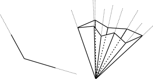
Figure 1: Conical polyhedral curtains in $\mathbb{R}^{2}$ and $\mathbb{R}^{3}$.

Our main examples of polyhedral curtains in $\mathbb{R}^{d}$ are $\Delta$-curtains in the sense of the following definition.

Definition 2.

Let $\Delta=\mbox{\em\rm conv}\{a_{0},a_{1},\ldots,a_{d}\}\subset\mathbb{R}^{d}$ be a non-degenerate simplex with the barycenter at the origin. For each pair $\theta=(F_{1},F_{2})$ of complementary faces of $\Delta$ there is a join decomposition $\Delta=F_{1}\ast F_{2}$. Assuming that both $F_{1}$ and $F_{2}$ are non-empty let $S^{d-2}_{\theta}=\partial(F_{1})\ast\partial(F_{2})\subset\partial(\Delta)$ be an associated $(d-2)$-dimensional, polyhedral sphere. A polyhedral hypersurface $H\subset\mathbb{R}^{d}$ is called a $\Delta$-curtain if for some $\theta=(F_{1},F_{2})$ and $x\in\mathbb{R}^{d}$

$$H=x+C_{\theta}=x+\mbox{\rm cone}(S^{d-2}_{\theta}).$$ (1)

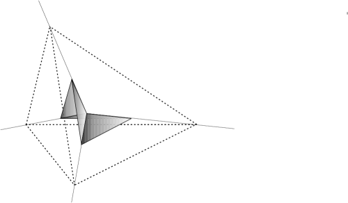
Figure 2: A fragment of a $\Delta$-curtain in $\mathbb{R}^{3}$.

The classical ham sandwich theorem claims that a collection of $d$ measurable sets in $\mathbb{R}^{d}$ admits a hyperplane bisector, i.e. a hyperplane that simultaneously cuts them in halves of equal measure. The following ‘polyhedral curtain theorem’ is formally a statement of similar nature where the role of hyperplanes is played by $\Delta$-curtains.

Theorem 3.

(Polyhedral curtain theorem) Suppose that $\Delta\subset\mathbb{R}^{d}$ is a simplex with the barycenter at the origin. Let $\mu_{1},\mu_{2},\ldots,\mu_{d}$ be a collection of continuous mass distributions (measures) on $\mathbb{R}^{d}$. Then there exists a $\Delta$-curtain $H=H_{(x,\theta)}$ which divides the space $\mathbb{R}^{d}$ into two ‘half-spaces’ $H^{+}$ and $H^{-}$ such that for each $j\in\{1,\ldots,d\}$,

$$\mu_{j}(H^{+})=\mu_{j}(H^{-}).$$

Remark 1.

In contrast with the ham sandwich theorem, Theorem 3 has a more combinatorial flavor, in this respect it resembles Radon’s and Tverberg theorem [20]. It will become clear from the proof that it is really an offspring of the multidimensional splitting necklace theorem [9], a higher dimensional generalization of the celebrated splitting necklace theorem of Alon, [1, 2].

2 Two dimensional case of Theorem 3

As a motivation for introducing $\Delta$-zonotopes (Section 3) and flat (polyhedral) complexes (Section 4), we outline the proof of the two dimensional case of the polyhedral curtain theorem (Theorem 3), emphasizing the main ideas and constructions. We will demonstrate that two (bounded) measurable sets $U$ and $V$ in the plane (say the simple shapes depicted in Figure 4) admit a fair division by a planar polyhedral curtain, with the directions of the rays prescribed in advance by a triangle $\Delta$. Without a loss of generality we assume that $U\cup V\subset\Delta$.

Theorem 3 is a ‘fair division theorem’, so like in other results of this type one is supposed to identify the associated ‘configuration space’ of allowed (admissible) divisions. For comparison, let us briefly review the construction of the configuration space for the two dimensional splitting necklace problem, [9, Section 2] (with $3$ vertical and $2$ horizontal axis aligned cuts). An admissible division of the square $I^{2}$, corresponding to the chosen sequences $0=x_{0}\leq x_{1}\leq x_{2}\leq x_{3}\leq x_{4}=1;0=y_{0}\leq y_{1}\leq y_{2}\leq y_{3}=1$, is depicted in Figure 3. It immediately follows that the configuration space of all divisions of $I^{2}$ (of the type $(3,2)$) is the product $\Delta^{3}\times\Delta^{2}$ of simplices.

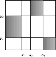
Figure 3: Division of the square with axis-aligned cuts.

Assuming that there are two persons involved in the division, we observe that there are $2^{12}$ possible scenarios for distributing these rectangles (one possibility is depicted in Figure 3). As a consequence, the configuration space $\Omega(3,2)$ of all divisions of the square of the type $(3,2)$, together with all possible allocations of rectangular pieces to two parties involved, is the union of $2^{12}$ polyhedral cells (copies of $\Delta^{3}\times\Delta^{2}$). These cells are glued together, along their boundaries, whenever some of the elementary rectangles degenerate (for example if $x_{i}=x_{i+1}$ or $y_{j}=y_{j+1}$), see [9, Section 2] for more details.

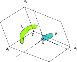
Figure 4: A division with a moving fan.

In the two dimensional case of the polyhedral curtain theorem, instead of the square, the basic shape (convex body) is a centrally symmetric hexagon, associated to the triangle $\Delta={\rm conv}\{a_{0},a_{1},a_{2}\}$, Figure 4. The axis-aligned cuts (of the square) are replaced by the dissection of the hexagon $Q$ into three regions, determined by the three rays emanating from the same point (the apex of the associated fan). The rays are always assumed to be translates of the basic system of rays (basic fan), generated by vectors $\{a_{0},a_{1},a_{2}\}$ with the apex at the origin $O$. The apex of the translated fan can be any point in the hexagon, including the boundary, so the configuration space of all such division is the hexagon $Q$ itself. There are $2^{3}=8$ possibilities to allocate the three regions, obtained by this division, to the two interested parties. As a result there are eight hexagons, each associated to one of possible eight scenarios for the division. These hexagons are glued together whenever one (or two) of the three regions degenerates, this happens if the apex $x$ is on the boundary of $Q$.

Summarizing, we observe that the configuration space encoding all admissible divisions, together with the associated division scenarios, is a cell complex obtained by gluing together eight identical copies of a convex body (hexagon $Q$) along their boundaries, following a specific gluing scheme. We denote this configuration space by $\mathbb{A}(Q,\mathcal{F},S)$ (see also Section 4) where $\mathcal{F}$ is the associated fan and $S=[2]=\{1,2\}$ the set of associated ‘colors’ (representing the parties involved in the division).

A moment’s reflection shows that $\mathbb{A}(Q,\mathcal{F},[2])$ is homeomorphic to the $2$-sphere. Moreover, the involution on the set $[2]$ (corresponding the parties interchanging their roles), defines an involution on the set of cells and on the configuration space $\mathbb{A}(Q,\mathcal{F},[2])$, which is easily identified as the usual antipodal action.

In order to complete the proof of the planar case of the polyhedral curtain theorem we construct a ‘test map’ $\phi:\mathbb{A}(Q,\mathcal{F},[2])\rightarrow\mathbb{R}^{2}$, testing the fairness of the chosen division-allocation. More explicitly, let $(x,s)\in\mathbb{A}(Q,\mathcal{F},[2])$, where $x$ is the apex of the associated fan $\mathcal{F}=\{F_{0},F_{1},F_{2}\}$ and $s:\mathcal{F}\rightarrow\{0,1\}$ is the associated allocation function. Let $X_{0}=\cup\{F_{i}\mid s(F_{i})=0\}$ and $X_{1}=\cup\{F_{i}\mid s(F_{i})=1\}$ be the associated polyhedral ‘half-planes’, the planar regions separated by the chosen polyhedral curtain. Then by definition,

$$\phi((x,s))=(m(X_{0}\cap U)-m(X_{1}\cap U),m(X_{0}\cap V)-m(X_{1}\cap V)).$$

This function is easily shown to be continuous. By construction $\phi(-z)=-\phi(z)$. Since the zeros of $\phi$ correspond to fair divisions, the planar case of the polyhedral curtain theorem follows as a consequence of the Borsuk-Ulam theorem.

Example 4.

(communicated by Siniša Vrećica) It is interesting that one cannot in general guarantee the existence of a bisecting $\Delta$-curtain for three measurable sets $U,V,W$, even if the rotations (isometries) of the $\Delta$-curtains are allowed. Indeed, the example is provided by small discs centered at the vertices of the triangle $\Delta$.

3 $\Delta$-zonotopes $R_{\Delta}$

Generalizing and developing the ideas from Section 2 we introduce $\Delta$-zonotopes as higher dimensional analogues of the centrally symmetric hexagon, used in the proof of the planar case of Theorem 3.

Definition 5.

Let $\Delta={\rm conv}\{a_{0},a_{1},\ldots,a_{d}\}$ be a non-degenerate simplex in $\mathbb{R}^{d}$ such that $a_{0}+\ldots+a_{d}=0$. The convex polytope, defined as the Minkowski sum,

$$R_{\Delta}=[0,a_{0}]+[0,a_{1}]+\ldots+[0,a_{d}]$$ (2)

is referred to as $\Delta$-zonotope. The simplex $\Delta$ is called the generating simplex of the polytope $R_{\Delta}$. Each polytope $R_{\Delta}$ has a ‘standard cubulation’ $R_{\Delta}=C_{0}\cup\ldots\cup C_{d}$ where $C_{i}$ is the parallelotope ($d$-parallelepiped) spanned by vectors $\{a_{j}\}_{j\neq i}$.

Figure 5: Rhombic dodecahedron and its generating simplex.

Two dimensional $\Delta$-zonotopes are the regular hexagon and its affine images. Figure 5 shows the rhombic dodecahedron, the $3$-dimensional $\Delta$-zonotope, together with its generating intervals (generating simplex). Recall that according to the classic classification of the mathematician, crystallographer, and mineralogist Evgraf Fedorov, rhombic dodecahedron is one of the five space filling polytopes known as parallelohedra. Rhombic dodecahedron is also the Voronoi cell of the face centered cubic lattice in the $3$-space.

Rhombic dodecahedron (and $\Delta$-zonotopes as its higher dimensional analogues) have appeared in a very interesting problem of Makeev [10] about universal covers of convex bodies of diameter $1$. Recall that the related result in dimension $2$ is one of the classics of the combinatorial geometry in the plane ([14]).

Conjecture 6.

(V.V. Makeev [10]) Every convex body $K$ in $\mathbb{R}^{d}$ of diameter $\leq 1$ can be covered by a translate of the convex body $R_{\Delta}$ for some non-degenerate simplex $\Delta$ of diameter $\leq 1$.

The conjecture was subsequently established in dimension $d=3$, independently by Makeev [11] (with mild assumptions on $K$), by Hausel, Makai, and Szücs [5], and by Kuperberg [6]. The original conjecture was formulated for the dual $D_{d}=(\Delta-\Delta)^{\circ}$ of the difference body of a simplex, rather than for the $\Delta$-zonotope $R_{\Delta}$. The added importance of the difference body $\Delta-\Delta={\rm conv}\{e_{i}-e_{j}\mid 0\leq n\}$ of the $d$-simplex $\Delta={\rm conv}\{e_{i}\}_{i=0}^{n}\subset\mathbb{R}^{n+1}$ stems from the fact that it can be described as the convex hull of the root system $A_{n}$. The following proposition shows the equivalence of these definitions of generalized rhombic dodecahedra.

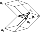
Figure 6: $\Delta$-zonotope $R_{\Delta}$ is the dual of $\Delta-\Delta$.

Proposition 7.

Let $\Delta={\rm conv}\{a_{0},a_{1},\ldots,a_{d}\}$ be a regular simplex in $\mathbb{R}^{d}$ such that $a_{0}+\ldots+a_{d}=0$. Let $H_{i,j}=\{x\in\mathbb{R}^{d}\mid|\langle x,a_{i}-a_{j}\rangle|\leq|\langle a_{i},a_{i}-a_{j}\rangle|\}$ be the region between two hyperplanes orthogonal to the edge $a_{i}-a_{j}$, passing respectively through the vertices $a_{i}$ and $a_{j}$. Then for some constant $\lambda>0$,

$$\lambda(\Delta-\Delta)^{\circ}=\bigcap_{i\neq j}H_{i,j}=R_{\Delta}.$$ (3)

Proof: (outline). Two parallelotopes $C_{0}$ and $C_{1}$ from the standard cubulation of $R_{\Delta}$ (Definition 5) are depicted in Figure 6. Let $P$ be the parallelotope generated by vectors $a_{2},\ldots,a_{d}$ and let $H$ be the associated hyperplane. Then $H$ is orthogonal to $a_{0}-a_{1}$ and the supporting hyperplanes $a_{0}+H$ and $a_{1}+H$ of $R_{\Delta}$ are precisely the boundary hyperplanes of $H_{0,1}$. $\square$

3.1 $\Delta$-zonotopes and quadrangulations

$\Delta$-zonotopes appear, at least implicitly, in toric topology in the context of standard quadrangulations (cubulations) of simple polytopes, see [3, Chapter 4]. Here we summarize one of this constructions, referring the reader to [3] for more details and other related information.

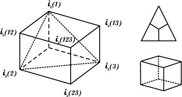
Figure 7: The front complex of a cube.

Each non-empty subset $I=\{j_{1},\ldots,j_{k}\}\subset[n]$ can be associated both a vertex $a_{I}=(1/k)(e_{j_{1}}+\ldots+e_{j_{k}})$ of the barycentric subdivision of the simplex $\Delta=\Delta^{n-1}={\rm conv}\{e_{1},\ldots,e_{n}\}$ and the vertex $b_{I}=e_{j_{1}}+\ldots+e_{j_{k}}$ of the standard cube $I^{n}\subset\mathbb{R}^{n}$. The correspondence $a_{I}\mapsto b_{I}$ is extended to a piecewise linear embedding $i_{c}:\Delta^{n-1}\rightarrow I^{n}$ which turns out to be an isomorphism of $\Delta^{n-1}$ with the ‘front face’ $F_{f}(I^{n})$ of the cube $I^{n}$ (Figure 7).

The front face $F_{f}(I^{n})$ is formally described as the union of all facets of $I^{n}$ which contain the vertex $b_{[n]}=e_{1}+\ldots+e_{n}$. A moment reflection shows that there exists a natural piecewise linear isomorphism $\nu:F_{f}(I^{n})\rightarrow R_{\Delta^{n-1}}$ of the front face $F_{f}(I^{n})$ and the $\Delta$-zonotope associated to $\Delta^{n-1}$. Indeed, the standard cubulation of $R_{\Delta^{n-1}}$ (Definition 5) is naturally brought into one-to-one correspondence with the natural cubulation of the front face of $I^{n}$.

Some of the properties of the piecewise linear isomorphisms $i_{c}$ and $\nu$, as well as their composition $I_{c}=\nu\circ i_{c}$,

$$I_{c}:\Delta^{n-1}\stackrel{{\scriptstyle i_{c}}}{{\longrightarrow}}F_{f}(I^{n})\stackrel{{\scriptstyle\nu}}{{\longrightarrow}}R_{\Delta^{n-1}},$$ (4)

are summarized in the following proposition.

Proposition 8.

The map $I_{c}$ described by (4) is a piecewise linear isomorphism which preserves the associated cubical decompositions (Figure 7). The standard cubulation $R_{\Delta^{n-1}}=C_{1}\cup\ldots\cup C_{n}$ (Definition 5) induces a decomposition

$$\partial(R_{\Delta^{n-1}})=F_{f}(C_{1})\cup\ldots\cup F_{f}(C_{n})$$

of the boundary of the $\Delta$-zonotope $R_{\Delta^{n-1}}$ into the associated front faces. This decomposition is well-behaved with respect to the isomorphism $I_{c}$ in the sense that $I_{c}(F_{i}(\Delta^{n-1}))=F_{f}(C_{i})$, where $\partial(\Delta^{n-1})=\cup_{i=1}^{n}~{}F_{i}(\Delta^{n-1})$ is the facet decomposition of the simplex $\Delta^{n-1}$.

4 Flat polyhedral complexes

A flat polyhedral complex $E$ arises if several copies of a convex polyhedron (convex body) $B$ are glued together along some of their common faces (closed convex subsets of their boundaries). By construction there is a ‘folding map’ $p:E\rightarrow B$ which resembles the moment map from toric geometry. Examples of flat polyhedral complexes include ‘small covers’ and other locally standard $\mathbb{Z}_{2}$-toric manifolds, but the idea can be also traced back (at least) to A.D. Alexandrov’s ‘flattened convex surfaces’.

A class of flat polyhedral complexes, modelled on a product of two or more simplices $B=\Delta^{p_{1}}\times\ldots\times\Delta^{p_{k}}$, was used in [9] for a proof of a multidimensional generalization of Alon’s ‘splitting necklace theorem’ [1]. Developing this idea we demonstrated in Section 1 that some new classes of flat polyhedral complexes naturally appear as ‘configuration spaces’, leading to new ‘fair division theorems’.

Here we introduce two classes of flat complexes, based on convex bodies (polyhedra) in $\mathbb{R}^{d}$ and develop their theory as far as it is needed for our central applications, including the proof of Theorem 3.

4.1 Convex fans and illumination systems

A convex fan $\mathcal{F}$ ([18]) is tacitly assumed to have the apex at the origin. Moreover, it is complete in the sense that it covers the whole of $\mathbb{R}^{d}$. For a given convex fan $\mathcal{F}$ in $\mathbb{R}^{d}$ let $\mathcal{F}_{max}=\{V_{1},V_{2},\ldots,V_{m}\}$ be the associated collection of maximal cones in $\mathcal{F}$. Since $\mathcal{F}$ is determined by $\mathcal{F}_{max}$, we shall (with a mild abuse of the language) often neglect the difference between $\mathcal{F}$ and $\mathcal{F}_{max}$ and sometimes write simply $\mathcal{F}=\{V_{1},V_{2},\ldots,V_{m}\}$. A translated fan is defined as $x+\mathcal{F}=\{x+V_{i}\}_{i=1}^{m}$.

There is a well known class of problems in classical combinatorial geometry known as illumination or visibility problems, see [12]. Motivated by this, a convex cone $V\subset\mathbb{R}^{d}$, with the apex at $a\in\mathbb{R}^{d}$ may be interpreted as the region in $\mathbb{R}^{d}$ illuminated by a light source (reflector) positioned at the point $a$. More generally, a fan $\mathcal{F}_{max}=\{V_{1},V_{2},\ldots,V_{m}\}$ can be interpreted as an ‘illumination system’ of essentially non-overlapping light sources, associated with the cones $V_{i}$.

Given a finite set of labels or colors $S$, the status or the state of the illumination system $\mathcal{F}_{max}=\{V_{1},V_{2},\ldots,V_{m}\}$ is a function $f:[m]\rightarrow S$ describing the state of each of the individual light sources. For example for $i\in[m]$, the associated value $f(i)$ may be interpreted as the color of the light chosen for the cone $V_{i}$ from the given set $S$ of colors. In the simplest case when $S=\{0,1\}$, the two possibilities naturally correspond to the status of the light source being turned on or turned off.

Summarizing, we observe that an illumination system is a pair $(\mathcal{F},S)$ where $\mathcal{F}$ is a complete fan of convex cones while $S$ the set of admissible colors for each of the individual light sources.

4.2 Illumination complexes $\mathbb{A}(K,\mathcal{F},S)$

Let us start with the following data:

• $K\subset\mathbb{R}^{d}$ is a convex polyhedron (or more generally a convex body);

• $\mathcal{F}$ is finite complex of convex cones in $\mathbb{R}^{d}$ (a convex fan);

• $S$ is finite set of ‘colors’.

The illumination complex $\mathbb{A}(K,\mathcal{F},S)$ is so designed to encode all possible ways of illuminating the body $K$ from some point $x\in K$ by the (translated) illumination system $(\mathcal{F},S)$. More precisely, a typical element of $\mathbb{A}(K,\mathcal{F},S)$ is a pair $(x,f)$ where $x\in K$ and $f:[m]\rightarrow S$ is a status of the illumination system $(\mathcal{F},S)$.

Figure 8: Elements of the illumination complex $\mathbb{A}(K,\mathcal{F},S)$.

The choice of $x\in K$ determines where in $K$ the illumination system should be positioned (translated) while the function $f:[m]\rightarrow S$ describes the chosen inner status of each of the individual light sources of the illumination system $(\mathcal{F},S)$.

In the example depicted in Figure 8 (a), the status function $f:[3]\rightarrow\{0,1\}$ dictates that the light is turned off in cones $V_{1}$ and $V_{2}$ and turned on in $V_{3}$. The three chosen positions of the point $x\in K$ (Figure 8 (b), (c) and (d)) illustrate typical situations that may occur. In (b) all three light sources illuminate a part of the interior of $K$. In (c) ${\rm int}(V_{2})\cap{\rm int}(K)=\emptyset$ which means that the inner status of the light source associated with the cone $V_{2}$ is no longer important and can be either $0$ or $1$. This observation is a motivation for making the identification of points $(x,f)$ and $(x,g)$ where $g:[3]\rightarrow\{0,1\}$ is the status function such that $f(i)=g(i)$ for $i\neq 2$.

After the informal description of the configuration space $\mathbb{A}(K,\mathcal{F},S)$ we are finally ready for a formal definition.

Definition 9.

The configuration space (cell complex) $\mathbb{A}(K,\mathcal{F},S)$ is by definition the identification space $(K\times X)/\sim$, where $X=Fun([m],S)$ is the set of all functions from the index set $[m]$ (of $\mathcal{F}$) to $S$ and $(x,f)\sim(y,g)$ if and only if, $x=y$ and $f(i)=g(i)$ for each $i\in[m]$ such that ${\rm int}(V_{i})\cap{\rm int}(K)\neq\emptyset$.

4.3 Modified illumination complex $\mathbb{B}(K,S)$

The construction of the modified illumination complex $\mathbb{B}(K,S)$ follows the same general pattern used in the case of $\mathbb{A}(K,\mathcal{F},S)$, with some important differences. First of all $K$ is assumed to be a convex polytope (in the previous case $K$ was allowed to be a convex body). Secondly, for each $x\in K$ there is an associated fan $\mathcal{F}_{x}=\mathcal{F}_{x}(K)$ (with the apex at $x$) where $\mathcal{F}_{x}=\{{\rm cone}(x,F)\mid F\mbox{ \rm is a proper face of }K\}$. Observe that if $x\in{\rm bd}(K)$, the dimension of the cone ${\rm cone}(x,F)$ is $d$ if and only if $F$ is a facet of $K$ such that $x\notin F$.

Summarizing, instead of a fan $\mathcal{F}$ which is prescribed in advance, and the associated translated fan $x+\mathcal{F}$, here we have a fan $\mathcal{F}_{x}$ with the moving apex $x$, generated by the facets of $K$.

If $F(K)=\{F_{i}\}_{i=1}^{m}$ is the set of all facets of $K$ then the status function describing the colors selected for each of the associated light sources is a function $f:[m]\rightarrow S$.

Definition 10.

The configuration space (cell complex) $\mathbb{B}(K,S)$ is by definition the identification space $(K\times X)/\sim$, where $X=Fun([m],S)$ is the set of all functions from the index set $[m]$ (indexing the facets of $\mathcal{F}$) to $S$ and $(x,f)\sim(y,g)$ if and only if, $x=y$ and $f(i)=g(i)$ for each $i\in[m]$ such that $x\notin F_{i}$.

4.4 The complex $\mathbb{B}(\Delta,S)$

Theorem 11.

Suppose that $\Delta={\rm conv}\{a_{0},a_{1},\ldots,a_{d}\}\subset\mathbb{R}^{d}$ is a non-degenerate simplex with the barycenter at the origin, and let $S$ be a finite, non-empty set (of colors). Then the associated $\mathbb{B}$-complex is homeomorphic to the join of $(d+1)$ copies of the $0$-dimensional complex $S$,

$$\mathbb{B}(\Delta,S)\cong S\ast S\ast\ldots\ast S=S^{\ast(d+1)}$$

Corollary 12.

If $S=\{0,1\}$ then the associated $\mathbb{B}$-complex $\mathbb{B}(\Delta,[2])$ is isomorphic to the $d$-sphere, the boundary $\partial\diamondsuit^{d}$ of the $d$-dimensional cross-polytope $\diamondsuit^{d}$.

Proof of Theorem 11: Suppose that the simplex $\Delta={\rm conv}\{a_{i}\}_{i=0}^{d}$ has volume $1$, $m(\Delta)=1$. Let us define a map,

$$\Phi:\mathbb{B}(\Delta,S)\rightarrow S^{\ast(d+1)}$$ (5)

and show that it is an isomorphism of simplicial complexes. Let $(x,f)\in\mathbb{B}(\Delta,S)$. Let $x=\alpha_{0}a_{0}+\ldots+\alpha_{d}a_{d}$ be the barycentric decomposition $x$ and let $F_{i}$ be the facet of $\Delta$, opposite to the vertex $a_{i}$, $F_{i}={\rm conv}\{a_{0},\ldots,\hat{a}_{i},\ldots,a_{d}\}$.

Lemma: The volume of the ‘pyramid’ $D_{i}(x):={\rm conv}(\{x\}\cup F_{i})$, with the apex at $x$ and the face $F_{i}$ as the base, is equal to the barycentric coordinate $\alpha_{i}$. In other words the knowledge of the volumes of all convex sets $D_{i}(x)$ allows us to determine uniquely the position of the point $x\in\Delta$.

By definition $\Phi(x,f)=\alpha_{0}f(0)+\alpha_{1}f(1)+\ldots+\alpha_{d}f(d)\in S^{\ast(d+1)}$. It is not difficult to see that this map is well defined and that it provides the desired isomorphism between $\mathbb{B}(\Delta,S)$ and $S^{\ast(d+1)}$. $\square$

4.5 Well illuminated complexes

Contrary to the case of the $\mathbb{B}$-complex (Theorem 11), the corresponding $\mathbb{A}$-complex $\mathbb{A}(\Delta,\mathcal{F},S)$, associated to the simplex $\Delta={\rm conv}\{a_{j}\}_{j=0}^{d}$, is quite irregular even if $\mathcal{F}$ is the fan $\mathcal{F}_{0}=\{{\rm cone\{F_{i}\}}\}_{i=0}^{d}$. The following definition clarifies which properties of $\mathbb{A}$-complexes should be considered ‘regular’, at least from the point of view of intended applications in this paper.

Definition 13.

Given a convex fan $\mathcal{F}$ in $\mathbb{R}^{d}$ and a finite set $S$ of colors, we say that a convex body $K\subset\mathbb{R}^{d}$ is $(\mathcal{F},S)$-well illuminated if the complex $\mathbb{A}(K,\mathcal{F},S)$ is $(d-1)$-connected.

Definition 14.

If $Q$ is a convex polytope such that $0\in{\rm int}(Q)$ there are two ‘tautological’ fans associated with $Q$. The first is the face fan,

$$\mathcal{F}_{Q}=\{{\rm cone}(F)\mid F\mbox{ {\rm is a proper face of} }Q\},$$ (6)

and the second is the normal fan $\nu(Q)$.

Problem 15.

For a given pair $(\mathcal{F},S)$ characterize convex bodies $K$ which are $(\mathcal{F},S)$-well illuminated in the sense of Definition 13. As a first step it would be interesting to know examples of well illuminated bodies, especially if $\mathcal{F}$ is one of the fans $\mathcal{F}_{Q}$ and $\nu(Q)$, associated to a convex body $Q$, and $S=\{0,1\}$ is a $2$-element set.

4.6 The complex $\mathbb{A}(R_{\Delta},\mathcal{F}_{\Delta},S)$

In this section we show that the centrally symmetric hexagon (in the plane), the rhombic dodecahedron (in the $3$-space) and their higher dimensional analogues $R_{\Delta}$ are all $(\mathcal{F}_{\Delta},S)$-well illuminated, if $\Delta$ is the associated ‘generating simplex’ (Definition 5).

Theorem 16.

Let $\Delta={\rm conv}\{a_{0},a_{1},\ldots,a_{d}\}$ be a non-degenerate simplex in $\mathbb{R}^{d}$ with the barycenter at the origin and let $R_{\Delta}$ be the associated $\Delta$-polytope (Definition 5). Let $S$ be a finite, non-empty set of colors. Let $\mathcal{F}_{\Delta}=\{{\rm cone}(F)\mid F\mbox{ {\rm is a proper face of} }\Delta\}$ be the fan generated by the facets of the simplex $\Delta$. Then,

$$\mathbb{A}(R_{\Delta},\mathcal{F}_{\Delta},S)\cong S\ast S\ast\ldots\ast S=S^{\ast(d+1)}.$$ (7)

Moreover, this isomorphism is equivariant with respect to any permutation of the colors $\pi:S\rightarrow S$. In particular if $S=\{0,1\}$, the corresponding $\mathbb{A}$-complex is homeomorphic to the $d$-sphere, the boundary of the cross-polytope, $\mathbb{A}(R_{\Delta},\mathcal{F}_{\Delta},[2])\cong\partial(\diamondsuit^{d})$.

Proof: Let $(x,f)\in\mathbb{A}(R_{\Delta},\mathcal{F}_{\Delta},S)$. Define $F_{i}={\rm conv}\{a_{0},\ldots,\hat{a}_{i},\ldots,a_{d}\}$ as the facet of $\Delta$, opposite to the vertex $a_{i}$, and let $\{{\rm cone}(F_{i})\}_{i=0}^{d}$ be the collection of maximal cones in $\mathcal{F}_{\Delta}$. The required isomorphism,

$$\Psi:\mathbb{A}(R_{\Delta},\mathcal{F}_{\Delta},S)\rightarrow S\ast S\ast\ldots\ast S=S^{\ast(d+1)}.$$ (8)

is defined by,

$$\Psi(x,f)=(1/\alpha)[\alpha_{0}f(0)+\alpha_{1}f(1)+\ldots+\alpha_{d}f(d)]$$ (9)

where $\alpha_{i}=\alpha_{i}(x,f)=m((x+{\rm cone}(F_{i}))\cap R_{\Delta})$ is the volume of the region in $R_{\Delta}$ illuminated by the cone $x+{\rm cone}(F_{i})$ and $\alpha=\alpha_{0}+\ldots+\alpha_{d}=m(R_{\Delta})$.

Lemma 17.

The map $\Psi$ is equivariant with respect to the group of all permutations of the set $S$ of colors.

Proof of Lemma 17: This is a consequence of the fact that the cell $C_{f}\subset\mathbb{A}(R_{\Delta},\mathcal{F}_{\Delta},S)$, associated to a function $f:\{0,\ldots,d\}\rightarrow S$, is mapped to the corresponding cell $D_{f}=\{f(0)\}\ast\ldots\ast\{f(d)\}\subset S^{\ast(d+1)}$. In other words $\Psi$ is the equivariant extension of the map $\psi:R_{\Delta}\rightarrow\Delta^{d}$, defined by

$$\psi(x)=\alpha_{0}a_{0}+\ldots+\alpha_{d}a_{d},$$ (10)

where $\alpha_{i}$ have the same meaning as in the equation (9). $\square$

In the following lemma we show that the map $\Psi$ defined by (9) is a monomorphism.

Lemma 18.

If $(x,f),(y,g)\in\mathbb{A}(R_{\Delta},\mathcal{F}_{\Delta},S)$ are distinct points then $\Psi(x,f)\neq\Psi(y,g)$.

Proof of Lemma 18: We can assume that $f=g$, indeed if $\alpha_{i}(x,f)\neq 0\neq\alpha_{i}(y,g)$ and $f(i)\neq g(i)$ then clearly $\Psi(x,f)\neq\Psi(y,g)$. Let us assume that $x$ is in the interior of $R_{\Delta}$. Since $\mathcal{F}_{\Delta}$ is a complete fan, $y-x\in{\rm cone}(F_{i})$ for some $i$. As a consequence,

$$(y+{\rm cone}(F_{i}))\cap{\rm int}(R_{\Delta}))\varsubsetneq(x+{\rm cone}(F_{i}))\cap{\rm int}(R_{\Delta})$$ (11)

which implies that $\alpha_{i}(y,f)<\alpha_{i}(x,f)$. A slight extension of this argument applies also in the case when both points $x$ and $y$ are on the boundary of $R_{\Delta}$. Indeed, a least one of the cones $V_{i}:=x+{\rm cone}(F_{i})$ such that $y-x\in V_{i}$ has the property $V_{i}\cap{\rm int}(R_{\Delta}))\neq\emptyset$ and the relation (11) is again satisfied. $\square$

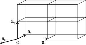
Figure 9:

Let us now show that $\Psi$ is an epimorphism. Since ${\rm Image}(\Psi)\subset S^{\ast(d+1)}$ is a closed set, it is sufficient to show that the image is everywhere dense in $S^{\ast(d+1)}$.

Lemma 19.

If $z\in S^{\ast(d+1)}$ has the representation $z=\beta_{0}z_{0}+\beta_{1}z_{1}+\ldots+\beta_{d}z_{d}\in S^{\ast(d+1)}$ such that $\beta_{i}\neq 0$ for each $i$, then for some $(x,f)\in\mathbb{A}(R_{\Delta},\mathcal{F}_{\Delta},S),\,\alpha_{i}(x,f)=\beta_{i}$.

Proof of Lemma 19: It is sufficient to show that the map $\psi:R_{\Delta}\rightarrow\Delta^{d}$, defined by (10) is an epimorphism. Let $\phi=\psi\circ I_{c}:\Delta^{d}\rightarrow\Delta^{d}$ where $I_{c}:\Delta_{d}\rightarrow R_{\Delta}$ is the map defined by (4) (Proposition 8). By inspection of the Figure 9 we observe that $\alpha_{i}(x)=0$ if $x\in F_{f}(C_{i})$, the front face of $C_{i}$, where $R_{\Delta}=C_{0}\cup\ldots\cup C_{d}$ is the standard cubulation of $R_{\Delta}$. From here and Proposition 8 it immediately follows that the map $\phi^{\prime}:\partial(\Delta^{d})\rightarrow\partial(\Delta^{d})$ is a homotopic to the identity map. By the standard argument, used in the proof of Brouwer’s fixed point theorem, it follows that ${\rm int}(\Delta^{d})\subset{\rm Image}(\phi)$ which in turn implies that $\psi$ is also an epimorphism. $\square$

Corollary 20.

In light of Theorem 11 the complexes $\mathbb{A}(R_{\Delta},\mathcal{F}_{\Delta},S)$ and $\mathbb{B}(\Delta,S)$ are equivariantly homeomorphic. Moreover, this homeomorphism is naturally defined in terms of the associated illumination systems.

5 Fair divisions by polyhedral cones

The general configuration space/test map-scheme (CS/TM-scheme) was used long before it was recognized in [19], as a key organizing principle for applying the topological methods on problems of combinatorial nature. According to this scheme [19, 20], the problem can be classified by the nature of its configuration space (the space of all reasonable ‘candidates for the solution’), and the nature of topological principles involved in its solution. The emphasis on ‘configuration spaces’ led to the systematization of tools for their analysis and construction and, as a useful byproduct, seemingly distant problems were recognized as neighbors or (topological) ‘genetic relatives’, see [13, 19, 20] for details and examples.

Following the CS/TM-scheme, the illumination complexes $\mathbb{A}(K,\mathcal{F},S)$ and $\mathbb{B}(K,S)$ were designed as configuration spaces suitable for applications to ‘envy-free’, ‘fair division’ or ‘consensus division’ theorems, where two or more parties are involved in dividing an object following the rules prescribed in advance (see [8] for an introduction and first examples, and [20] for an overview). In this section we formulate and prove these fair division results.

As in Section 4 the simplex $\Delta={\rm conv}\{a_{j}\}_{j=0}^{d}\subset\mathbb{R}^{d}$ is assumed to be non-degenerate with barycenter at the origin, and $\mathcal{F}_{\Delta}=\{{\rm cone}(F_{i})\}_{i=0}^{d}$ is the associated ‘face-fan’ determined by the facets $F_{i}$ of $\Delta$ (Definition 14).

Theorem 21.

Choose positive integers $n,q$ such that $q=p^{k}$ is a power of a prime $p\geq 2$ and let $d=n(q-1)$. Let $\mu_{1},\mu_{2},\ldots,\mu_{n}$ be a collection of continuous measures on $\mathbb{R}^{d}$ with finite support. Then there exists a translate $x+\mathcal{F}_{\Delta}=\{x+{\rm cone}(F_{i})\}_{i=0}^{d}$ of the face fan of $\Delta$ and an allocation function $\theta:\{0,1,\ldots,d\}\rightarrow\{1,\ldots,q\}$ such that for each $\mu_{i}$ and all $j=1,2,\ldots,q$,

$$\sum_{\theta(\nu)=j}\mu_{i}(x+{\rm cone}(F_{\nu}))=(1/q)\mu_{i}(\mathbb{R}^{d}).$$ (12)

Proof: Without loss of generality (by a homothetic enlargement of the simplex $\Delta$) we can assume that the supports of all measures $\mu_{i}$ are contained in $\Delta$. Let $R_{\Delta}$ be the $\Delta$-zonotope associated to $\Delta$ (Section 3) and let $\mathbb{A}(R_{\Delta},\mathcal{F}_{\Delta},S)$ be the associated illumination complex (Section 4.2) where $S=[q]$ is the chosen set of ‘colors’.

Recall that an element $(x,f)\in\mathbb{A}(R_{\Delta},\mathcal{F}_{\Delta},S)$ is a pair of a point $x\in R_{\Delta}$ and a status function $f:\{x+V_{i}\}_{i=0}^{d}\rightarrow[q]$ of the illumination system $x+\mathcal{F}=\{x+V_{i}\mid 0\leq i\leq d\}$, where $V_{i}={\rm cone}(F_{i})$.

For each pair of indices $i\in[n]$ and $j\in[q]$, define $\alpha_{i,j}=\alpha_{i,j}(x,f)$ by

$$\alpha_{i,j}=\alpha_{i,j}(x,f)=\sum_{\theta(\nu)=j}\mu_{i}(x+{\rm cone}(F_{\nu})).$$ (13)

The function $\alpha_{i,j}:\mathbb{A}(R_{\Delta},\mathcal{F}_{\Delta},S)\rightarrow\mathbb{R}$ is well-defined and continuous. The associated matrix valued function

$$\Phi:\mathbb{A}(R_{\Delta},\mathcal{F}_{\Delta},S)\rightarrow{\rm Mat}_{n\times q}(\mathbb{R}),\,\Phi(x,f)=A=(\alpha_{i,j})$$

is $\Sigma_{q}$-equivariant with respect to the action which permutes the columns of the matrix $A=(\alpha_{i,j})$. Observe that the unique fixed point of this action is the matrix $O=(\omega_{i,j})$ such that $\omega_{i,j}=(1/q)\mu_{i}(\mathbb{R}^{d})$ for each $i$ and $j$. Observe that ${\rm Image}(\Phi)\subset L$ where $L\subset{\rm Mat}_{n\times q}(\mathbb{R})$ is a $\Sigma_{q}$-invariant affine subspace define by equations,

$$\sum_{j=1}^{q}~{}x_{i,j}=\mu_{i}(\mathbb{R}^{d})\quad\mbox{ {\rm for each} }\,i=1,\ldots,n.$$

The dimension of this space is $n(q-1)$ and if (12) is never satisfied there arises a $\Sigma_{q}$-equivariant map,

$$\Psi:\mathbb{A}(R_{\Delta},\mathcal{F}_{\Delta},S)\rightarrow S(L)$$

where $S(L)$ is the $[n(q-1)-1]$-dimensional unit sphere in $L$. Since by Theorem 16 the complex $\mathbb{A}(R_{\Delta},\mathcal{F}_{\Delta},S)$ is $(d-1)$-connected, the existence of such a map would be in contradiction with the following general Borsuk-Ulam type theorem (Theorem 22).

Theorem 22.

([17, 15, 7, 19, 13, 8]) Suppose that $p\geq 2$ is a prime number and let $G=\mathbb{Z}_{p}^{\times k}$ be the elementary abelian group of order $p^{k}$. Assume that $X$ and $Y$ are fixed-point free $G$-spaces such that $X$ is $n$-connected and $Y$ is a $n$-dimensional sphere. Then there does not exist a $G$-equivariant map $f:X\rightarrow Y$.

Theorem 21 relied in essential way on the properties of the complex $\mathbb{A}(R_{\Delta},\mathcal{F}_{\Delta},S)$. A $\mathbb{B}(K,S)$-counterpart of that result is the following theorem.

Theorem 23.

Choose positive integers $n,q$ such that $q=p^{k}$ is a power of a prime $p\geq 2$ and let $d=n(q-1)$. Let $\Delta\subset\mathbb{R}^{d}$ be a non-degenerate simplex. Assume that $\mu_{1},\mu_{2},\ldots,\mu_{n}$ are continuous measures on $\mathbb{R}^{d}$ with finite support ${\rm Supp}(\mu_{i})\subset\Delta$ . Then there exists a point $x\in\Delta$ and an allocation function $\theta:\{0,1,\ldots,d\}\rightarrow\{1,\ldots,q\}$ such that for each $\mu_{i}$ and all $j=1,2,\ldots,q$,

$$\sum_{\theta(\nu)=j}\mu_{i}({\rm cone}(x,F_{\nu}))=(1/q)\mu_{i}(\mathbb{R}^{d})$$ (14)

where ${\rm cone}(x,F_{\nu})$ is the cone with the apex $x$ generated by the facet $F_{i}$.

Proof: The proof is similar to the proof of Theorem 21 with the Theorem 11 used instead of Theorem 16. The details are left to the reader. $\square$

The proof of Theorem 23 is somewhat simpler than the proof of Theorem 21 since the associated configuration space is simpler. Nevertheless, Theorem 21 can be deduced from Theorem 23 by a limit and compactness argument.

Proposition 24.

Theorem 23 implies Theorem 21.

Proof: (outline) Let us suppose that the supports of all measures $\mu_{i}$ are contained in the ball $B(0,r)$, i.e. that $\mu_{i}(\mathbb{R}^{d}\setminus B(0,r))=0$ for each $i=1,\ldots,n$. Enlarge the simplex $\Delta$ by a homothety so that its diameter $R$ is much larger than $r$, $R\gg r$. By Theorem 23 there exists a pair $(x,f)\in\mathbb{B}(\Delta,S)$ which describes a fair dissection in the sense of the equation (14). There exists a constant $C>1$ such that if $x\notin B(0,Cr)$ then for at least one $\nu\in\{0,\ldots,d\}$ the cone ${\rm cone}(x,F_{\nu})$ does not intersect $B(0,r)$. It follows that if $(x,f)$ is a fair division then $x\in B(0,Cr)$. Since $R\gg Cr$ we observe that the cones ${\rm cone}(x,F_{\nu})$ and $x+{\rm cone}(F_{\nu})$ are very close so by a limit and compactness argument the condition (12) can be also satisfied. $\square$

6 Proofs of the polyhedral curtain theorem

The ‘polyhedral curtain theorem’ (Theorem 3) is a special case of Theorem 21 for $q=2$, i.e. if there are only two parties involved in the fair division. Indeed, a polyhedral curtain is nothing but the common boundary of two polyhedral sets,

$$\bigcup_{\theta(\nu)=1}(x+{\rm cone}(F_{\nu}))\quad\mbox{\rm and}\quad\bigcup_{\theta(\nu)=2}(x+{\rm cone}(F_{\nu})).$$

The reader interested only in the polyhedral curtain theorem may use the Borsuk-Ulam theorem (along the lines of the proof of the two dimensional case in Section 2) together with the $S=\{0,1\}$ case of Theorem 16 which claims that

$$\mathbb{A}(R_{\Delta},\mathcal{F}_{\Delta},[2])\cong\partial(\diamondsuit^{d})\cong S^{d-1}.$$

A further simplification can be achieved if one uses Theorem 11 together with the Borsuk-Ulam theorem, and the limiting/compactness argument used in the proof of Proposition 24.

7 Applications

The ‘polyhedral curtain theorem’ (Theorem 3) is a more combinatorial version od the ham sandwich theorem since it involves alternatives.

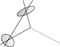
Figure 10: Ham sandwich and polyhedral curtain equipartitions.

For example in Figure 10 we see an equipartition of two measurable sets by a line and by one of three planar ‘curtains’ determined and prescribed in advance by the chosen triangle $\Delta$.

It can be expected that some standard applications of the ham sandwich theorem and its generalizations admit a modification involving the polyhedral curtain theorem and its extensions. In this section we offer only one example leaving a more complete discussion for subsequent versions of this paper.

7.1 Fair divisions by polynomial splines

One of the standard and useful extensions (consequences) of the ham sandwich theorem is the Stone-Tukey ‘polynomial ham sandwich theorem’, [16]. The key idea is to use some version of the monomial Veronese embedding $V:\mathbb{R}^{n}\rightarrow\mathbb{R}^{N}$ and read off the consequences in $\mathbb{R}^{n}$ of the ham sandwich theorem applied in $\mathbb{R}^{N}$. Here we apply a similar strategy to obtain consequences of the polyhedral curtain theorem.

For illustration we begin with an example. Let $W:\mathbb{R}^{2}\rightarrow\mathbb{R}^{3}$ be the embedding defined by $W(x,y)=(x,y,x^{2}+y^{2})$ and let $\pi:\mathbb{R}^{3}\rightarrow\mathbb{R}^{2},\,\pi(x,y,z)=(x,y)$ be the projection. Suppose that $X_{1},X_{2},X_{3}$ are measurable sets in $\mathbb{R}^{2}$ and let $Y_{i}=W(X_{i})$ be their images in the paraboloid $\Gamma\subset\mathbb{R}^{3}$, described by the equation $z=x^{2}+y^{2}$.

An application of the polyhedral curtain theorem in $\mathbb{R}^{3}$ on the sets $\{Y_{i}\}_{i=1}^{3}$ yields a piecewise circular curve (a circular spline) which cuts each of the sets $X_{i}$ in two parts of equal measure. The number of nodes of the spline is controlled by the number of faces in the polyhedral curtain.

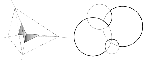
Figure 11: A circular spline associated to a polyhedral curtain.

Actually much more precise information about the spline can be deduced from the simplex $\Delta\subset\mathbb{R}^{3}$. Indeed, the slopes of the polyhedral faces of the curtain can be to some extent prescribed in advance by the shape of the generating tetrahedron $\Delta\subset\mathbb{R}^{3}$. Moreover, the $\pi$-images $\pi(L_{i}\cap\Gamma)$ of the (non-empty) intersections of two parallel planes $L_{1}$ and $L_{2}$ with the paraboloid $\Gamma$ are two concentric circles in $\mathbb{R}^{2}$.

From here we deduce that the splines can be chosen to be ‘concentric’ to one of seven circular splines which are prescribed in advance by the choice of the tetrahedron $\Delta$. These splines are referred to as $\Delta$-generated.

Proposition 25.

Suppose that $X_{1},X_{2},X_{3}\subset\mathbb{R}^{2}$ are three measurable sets in the plane. Then for each simplex $\Delta\subset\mathbb{R}^{3}$ there exists a $\Delta$-generated circular spline which cuts in half each of the measurable sets $X_{i}$.

References

- [1] N. Alon. Splitting necklaces. Advances in Math., 63:247–253, 1987.
- [2] N. Alon. Non-constructive proofs in combinatorics. Proc. Int. Congr. Math., Kyoto/Japan 1990, Vol. II(1991), 1421–1429.
- [3] V.M. Buchstaber, T. Panov. Torus Actions and Their Applications in Topology and Combinatorics, AMS, 2002.
- [4] A. Dold. Simple proofs of some Borsuk -Ulam results. Contemp. Math., 19:65 -69, 1983.
- [5] T. Hausel, E. Makai Jr., and A. Szücs. Inscribing cubes and covering by rhombic dodecahedra via equivariant topology. Mathematika, Vol. 47, Issue 1-2, December 2000, pp. 371–397. arXiv:math/9906066v2 [math.MG].
- [6] G. Kuperberg. Circumscribing constant-width bodies with polytopes, New York J. Math. 5 (1999), 91–100. arXiv:math/9809165v3 [math.MG].
- [7] M. de Longueville. Notes on the topological Tverberg theorem. Discrete Math., 241(1-3):207 -233, 2001.
- [8] M. de Longueville. A Course in Topological Combinatorics. Universitext, Springer New York, 2013.
- [9] M. de Longueville, R.T. Živaljević. Splitting multidimensional necklaces. Adv. Math. 218 (3): 926–939, 2008.
- [10] V.V. Makeev. Inscribed and circumscribed polyhedra to a convex body. (Russian) Mat. Zametki 55(4) (1994), 128–130, (English) Math. Notes 55 (1994), 423–425, MR 95h:52002.
- [11] V.V. Makeev, On affine images of a rhombo-dodecahedron circumscribed about a three-dimensional convex body. (Russian) Zapiski Nauchnykh Seminarov POMI, Vol. 246, 1997, pp. 191 -195. (English) Journal of Mathematical Sciences, June 2000, Vol. 100, Issue 3, pp. 2307–2309.
- [12] H. Martini, V. Soltan. Combinatorial problems on the illumination of convex bodies, Aequationes Math. 57 (1999) 121–152.
- [13] J. Matoušek, Using the Borsuk-Ulam Theorem. Lectures on Topological Methods in Combinatorics and Geometry, 2nd edition, Springer, 2007.
- [14] J. Pál, Über ein elementares Variationsproblem, Kgl. Danske Vid. Selskab., Mat–Fys. Medd. 3 (1920), 3–35, Jahrbuch Fortschr. Math. 47 (1919–1920), 684.
- [15] K.S. Sarkaria. Tverberg partitions and Borsuk -Ulam theorems. Pacific J. Math., 196:231 -241, 2000.
- [16] A.H. Stone, J.W. Tukey. Generalized sandwich theorems, Duke Mathematical Journal, 9: 356 -359.
- [17] A.Yu. Volovikov. On a topological generalization of the Tverberg theorem. Math. Notes, 59(3):324 -326, 1996. Translation from Mat. Zametki 59, No.3, 454–456 (1996).
- [18] G. Ziegler. Lectures on Polytopes, Graduate Texts in Mathematics 152, Berlin, New York: Springer-Verlag, 1995.
- [19] R.T. Živaljević. User’s guide to equivariant methods in combinatorics, I and II. Publ. Inst. Math. (Beograd) (N.S.), (I) 59(73), 1996, 114–130 and (II) 64(78), 1998, 107–132. Electronic versions available at, http://elib.mi.sanu.ac.rs/pages/browse_publication.php?db=publ.
- [20] R.T. Živaljević. Topological methods. Chapter 14 in Handbook of Discrete and Computational Geometry, J.E. Goodman, J. O’Rourke, eds, Chapman & Hall/CRC 2004, 305–330.