THE SPATIOKINEMATICAL STRUCTURE OF H₂O AND OH MASERS IN THE “WATER FOUNTAIN” SOURCE IRAS 18460$-$0151

Abstract

Using the Very Long Baseline Array and the European VLBI Network, we have observed 22.2 GHz H₂O and 1612 MHz OH masers in the water fountain source IRAS 18460$-$0151. The H₂O maser spectrum has a very wide line-of-sight velocity range ($\approx$310 km s^-1) and consists of three groups of emission features at the blue-shifted ($-68$ km s^-1$\lesssim$ $V_{\mbox{\scriptsize LSR}}$$\lesssim-17$ km s^-1) and red-shifted ($V_{\mbox{\scriptsize LSR}}$$\simeq$240 km s^-1) edges as well as around the systemic velocity (112 km s^-1$\lesssim$ $V_{\mbox{\scriptsize LSR}}$$\lesssim$133 km s^-1). The first two H₂O spectral components exhibit a highly-collimated high-velocity bipolar jet on the sky, with an angular separation of $\approx$120 milliarcseconds (mas) (240 AU in linear length) and a three-dimensional flow velocity of $\approx$160 km s^-1. The flow dynamical age is estimated to be only $\approx$6 yr (at the time of the observation epochs of 2006–2007). Interestingly, the systemic velocity component clearly exhibits a spherically-expanding outflow with a radius of $\approx$36 AU and a flow velocity of $\approx$9 km s^-1. On the other hand, the OH maser spectrum shows double peaks with a velocity separation of $\approx$25 km s^-1($V_{\mbox{\scriptsize LSR}}$$=$111–116 and 138–141 km s^-1), as typically seen in circumstellar envelopes of OH/IR stars. The angular offset between the velocity-integrated brightness peaks of the two high-velocity H₂O components is $\approx$25 mas (50 AU). The offset direction and the alignment of the red-shifted maser spots are roughly perpendicular to the axis of the H₂O maser flow. High-accuracy astrometry for the H₂O and OH masers demonstrates that the collimated fast jet and the slowly expanding outflow originate from a single or multiple sources which are located within 15 mas (30 AU). On the other hand, the estimated systemic velocity of the collimated jet ($V_{\rm sys}\approx$87–113 km s^-1) has a large uncertainty. This makes it difficult to provide strong constraints on models of the central stellar system of IRAS 18460$-$0151.

1 INTRODUCTION

“Water fountain” sources (WFs) are asymptotic giant branch (AGB) or post-AGB stars that host highly-collimated, fast ($V_{\rm exp}\gtrsim$50 km s^-1), bipolar jets traced by 22.2 GHz H₂O maser emission. Interestingly, all of the observed dynamical ages of the WF jets are less than 100 yr. As of 2013, 15 sources have been identified as possible WFs (in more detail, see Imai 2007; Desmurs et al. 2012). It is expected that they are signposts of the transition phase from the AGB to post-AGB, when one can see ignition of a stellar jet and a resulting metamorphosis from spherically symmetric to asymmetric structure of the circumstellar envelope (CSE).

Here we focus our interest on some WFs, in which H₂O masers near the dynamical centers of the jets show lower expansion velocities, roughly equal to a typical expansion velocity of a CSE in the AGB phase ($V_{\rm exp}\lesssim$30 km s^-1), and exhibit spherical symmetric distributions. The spherical expansion in such an expansion velocity is well traced in AGB CSEs by 1612 MHz OH maser emission (see, e.g., the stellar OH maser data base, Engels 2012). They are a completely different component from the collimated WF jet whose velocity often exceeds 100 km s^-1 (e.g., Imai et al. 2002; Imai 2007). For these interesting WFs, it is considered that they still host relic CSEs made at the end of the AGB phase because the majority of WFs are strongly obscured in the near-infrared bands (e.g. Deguchi et al. 2007). On the other hand, it is also considered that the stellar mass loss rate in the AGB phase will increase over $\dot{M}\geq 10^{-7}\>M_{\sun}{\rm yr}^{-1}$ or much higher (Bowers & Johnston, 1994). A WF likely appears when the mass loss rate of the AGB CSE reaches its maximum, but what will happen to the CSE soon after this phase? Thus, the exploration of the inner part of CSEs, including the OH and low-velocity H₂O masers, is important for identifying the stellar evolutionary phase through diagnosing the kinematics of such stellar mass loss. Eventually, the study of the WFs will provide important clues to understanding the mechanisms of stellar jet launching and planetary nebula shaping in terms of the AGB to post-AGB transition.

In this paper, we present the spatiokinematics of H₂O masers and their spatial relationship with the 1612 MHz OH maser emission associated with IRAS 18460$-$0151 (hereafter abbreviated as I18460), as revealed by observations with the Very Long Baseline Array (VLBA) and the European VLBI Network (EVN). The preliminary results were reported by Imai (2007) and Imai et al. (2008). Here we describe the results in more detail. This paper also presents additional data of the I18460 H₂O masers that were used for determining the secular proper motion of I18460. I18460 was first identified as a WF by Deguchi et al. (2007). The H₂O maser spectrum showed a very large velocity separation of $\approx$290 km s^-1, centered at the local-standard-of-rest (LSR) velocity of $V_{\mbox{\scriptsize LSR}}$$\approx$100 km s^-1. It also showed the systemic velocity component, whose velocity ($V_{\mbox{\scriptsize LSR}}$$\approx$120 km s^-1) coincides with that of the intrinsic CO emission of I18460 (Rizzo et al., 2012) and the center velocity of the double-peaked spectrum of OH masers (Sevenster et al., 1997). Such a systemic velocity component of H₂O maser emission has sometimes been observed in the archetypal WF source, W43A (Imai et al., 2002; Imai, 2007). It has been unclear with what that component is associated, candidates are either a relic AGB CSE as defined above or an “equatorial” flow. The latter has an expansion velocity ($v_{\rm exp}\gtrsim 30$ km s^-1) higher than that of the former ($v_{\rm exp}\approx$10–20 km s^-1). The existence of an equatorial flow in a WF was recognized in the spatiokinematical structure of SiO masers in W43A (Imai et al. 2005 (see also the case of IRAS 16342$-$3814, Sahai et al. 1999) ), but its origin is still obscure because of limited data from such flows. In IRAS 18286$-$0959, Paper II also recognized the existence of a similar flow, but H₂O maser features associated with the flow were considered as “outliers” of the collimated jet, which show proper motions much slower than those in the jet. In the case of I18460, we revealed the spatiokinematics of H₂O masers in the systemic velocity components in detail for the first time in WFs. In this paper, we adopt a distance to I18460 of $\sim$2 kpc (see Section 3.2), which is considerably less than the kinematic distance derived by assuming a circular orbit in the Milky Way (6.0 or 7.8 kpc).

Section 2 describes the VLBA and EVN observations of the H₂O and OH masers in I18460, respectively, including normal maser source mapping and phase-referencing astrometric procedures. Section 3 presents the H₂O and OH maser maps and the results of astrometry. Section 4 discusses the slowly expanding flow of I18460, whose spatiokinematical structure is clearly elucidated, and the secular motion of I18460 in the Milky Way, which may provide an important clue to revealing the character of the central star in I18460.

2 OBSERVATIONS AND DATA REDUCTION

We describe the VLBA and EVN observations (project codes BI033 and EI009, respectively) and the analyses of their data, which follow the same procedure as those in Paper II. We also describe the astrometry of the H₂O masers conducted in other VLBA observations (BI036).

2.1 VLBA Observations of the H₂O Masers

Table 1 summarizes the status of the VLBA observations and data reduction of the I18460 H₂O masers. VLBA observations were conducted three times during 2006 September–2007 February (BI033) and three times during 2008 September–2009 February (BI036). In the first set of observations, another H₂O maser source IRAS 18286$-$0959 was also observed at the same time Imai et al. (2013b) (hereafter Paper II), therefore the on-source time for I18460 was limited to 3 hr. In the second set of observations, the antenna-nodding, phase-referencing technique was employed for astrometry of the I18460 H₂O masers, in which the maser and the phase-reference source J185146.7$+$003532 (hereafter abbreviated as J1851, 2^∘.52 away from I18460) were observed in a source-switching cycle of one minute. In all of the six sessions, the continuum source OT 081 was also observed for 4 minutes in every 20 minutes for calibration of group-delay residuals and bandpass characteristics. The received signals were recorded at a rate of 128 Mbits s^-1 with 2 bit quantization into eight base-band channels (BBCs) in dual circular polarization. The centers of four pairs of BBCs, each of which has a bandwidth of 4 MHz, were set to LSR velocities of $-$55, 0, 120, and 240 km s^-1. The recorded data were correlated with the Socorro FX correlator using an integration period of 2 s. The data of each BBC was divided into 256 spectral channels, yielding a velocity spacing of 0.21 km s^-1 per spectral channel. The following coordinates were adopted as the delay-tracking centers in the data correlation:

$\alpha_{\rm J2000}=$18^h48^m42^s.94, $\delta_{\rm J2000}=$ $-$01^∘48^′30$\farcs$28 and

$\alpha_{\rm J2000}=$18^h48^m43^s.027, $\delta_{\rm J2000}=$ $-$01^∘48^′30$\farcs$46 for I18460 for the first and second sets of three sessions, respectively, and

$\alpha_{\rm J2000}=$18^h51^m46^s.723080, $\delta_{\rm J2000}=$ $+$00^∘35^′32$\farcs$36283 for J1851.

For the data reduction, we used the NRAO’s AIPS package and employed a normal procedure. After calibration of group-delay residuals and bandpass characteristics using scans on OT 081, fringe fitting and self-calibration were made using a spectral channel that contained bright maser emission. Column 3 in Table 1 gives the LSR velocity of the spectral channel selected as phase- and position-reference. The obtained solutions of calibration were applied to the data in all spectral channels. Finally, image cubes of the maser source were synthesized in visibility deconvolution through the CLEAN algorithm. Because most of the H₂O maser spots (velocity components) were spatially partially resolved, calibration solutions and the associated visibilities were missing from relatively long baselines ($B_{\lambda}\gtrsim{\rm 200~{}M}\lambda$) in the image synthesis. As a result, naturally weighted visibilities associated with available self-calibration solutions yielded a typical synthesized beam of 1.5 mas$\times$1.0 mas. Columns 4 and 5 of Table 1 give values of the 1 $\sigma$ noise level and the synthesized beam pattern, respectively.

In each spectral channel of the synthesized image cube, using a POPS pipeline script including the AIPS task SAD, brightness peaks higher than 7 $\sigma$ noise level were identified as maser spots and their parameters as Gaussian brightness components were extracted. We determined the position of a maser feature, which is a physical maser clump consisting of a cluster of maser spots seen in consecutive velocity components and at almost the same position within the synthesized beam, as described in Imai, Deguchi, & Sasao (2002). The peak-brightness velocity of a feature was determined by quadratic fitting of the peak intensities of the brightest three spots in the feature, then the position of the corresponding peak velocity was determined from linear interpolation of the positions of the two brightest spots.

For the astrometry of the I18460 H₂O masers, in the sessions of 2008–2009, all phase calibration steps were made using the data of J1851, the solutions were then applied to the data of I18460. Because the calibration of unknown zenith delay residuals was imperfect and I18460 is very close to the celestial equator, the synthesized maser source images were partially defocused, especially in the north–south direction. However, the obtained position accuracy of the H₂O masers ($\sim$0.1 mas and $\sim$0.5 mas in the right ascension (R.A.) and declination directions (decl.), respectively) is sufficient to measure the linear proper motions of the masers and to compare their coordinates with those of the OH masers. For measurement of relative maser proper motions, we used the image cube obtained from the astrometric analysis rather than that from the self-calibration scheme mentioned above.

2.2 EVN Observation of the OH Masers

The EVN observation of the I18460 OH masers ($F_{j}=1^{+}\rightarrow 2^{-1}$ ${}^{2}\Pi_{3/2}$ at 1.612231f GHz) (project code EI009B) was conducted on 2007 June 11 using the following telescopes: Lovell 76 m in Jodrell Bank, Cambridge 32 m, Westerbork Synthesis Radio Telescope (14 25-m), Medicina 32 m, Noto 32 m, Effelsberg 100 m, Onsala 25 m, Torun 32 m, and Hartebeesthoek 26 m. We used the antenna-nodding phase-referencing technique (e.g., Beasley & Conway 1995) to obtain astrometric measurements for the maser source. This was possible for every telescope except the Lovell 76 m, which always observed I18460 without antenna nodding. I18460 and the phase-reference continuum emission source J183307.8$+$013511 (hereafter abbreviated as J1833) were scanned in a source-switching cycle of 5 minutes, resulting in the total duration of scans on I18460 being $\sim$3 hr. J183243.5$+$135744 was observed for 3 minutes in every 40 minutes for calibration of group-delay residuals and bandpass characteristics. The received signals were recorded at a rate of 128 Mbits s^-1 with 2 bit quantization into eight BBCs in dual circular polarization. One pair of BBCs had a bandwidth of 1 MHz and others have 4 MHz for observing the I18460 H₂O maser and the J1833 continuum emission, respectively.

The recorded data were correlated with the Mark IV processor in the Joint Institute for VLBI in Europe using an integration period of 4 s. The data of each BBC was divided into 512 and 32 spectral channels, respectively, for the maser and continuum observations. A velocity channel spacing of 0.36 km s^-1 was obtained for the maser data. The coordinates of I18460 adopted in the data correlation were the same as the first set of the coordinates for the VLBA data (Section 2.1). The following coordinates for J1833 were used in the data correlation:

$\alpha_{\rm J2000}=$18^h33^m07^s.760875,

$\delta_{\rm J2000}=$ $+$01^∘15^′35$\farcs$30098.

In the analysis of the EVN data, in addition to the standard calibration procedures as described in Section 2.1, calibration of residual delays due to the ionosphere was also applied using the AIPS task TECOR. Fringe fitting and self-calibration were carried out as done for our VLBA observations but using the data of J183243.5$+$135744. Phase referencing, fringe fitting and self-calibration were undertaken using the data of J1833. The calibration solutions were applied to the data of I18460. The image of J1833 and the image cube of the OH maser source were synthesized in visibility deconvolution through the CLEAN algorithm. Calibration solutions and their associated visibilities were lost from long baselines ($B_{\lambda}\gtrsim{\rm 10~{}M}\lambda$) on J1833, which has an extended structure; this resulted in a large beam size for the image synthesis of the OH maser source. Through the phase-referencing technique, we synthesized a maser image cube (referred to as the phase-referencing-based cube) and determined the absolute coordinates of the OH maser source.

In addition, in order to obtain a higher angular resolution image cube of the OH maser source, free from the effects of the extended structure of J1833, fringe fitting and self-calibration were also carried out using the OH maser data. The spectral channel at $V_{\mbox{\scriptsize LSR}}$$=$111.7 km s^-1 was used as phase reference. The uniformly weighted visibilities yielded a synthesized beam of 97 mas$\times$23 mas at a P.A.$=$ 11°. Thus we generated another maser image cube (referred to as the self-calibration-based cube). The OH masers were also spatially resolved on baselines to the Hartebeesthoek station, causing the elongated beam pattern in the north–south direction.

3 RESULTS

Tables 2 and 3 give the parameters of H₂O maser features detected in the observation sessions in 2006–2007 and 2008–2009, respectively. In Table 3, the positions are given as offsets with respect to the phase-tracking center of I18460.

With LSR velocity and proper motion measurements, the three-dimensional spatiokinematics of the H₂O masers has been revealed. Table 4 gives the list of relative proper motions of H₂O maser features found in all observations. Note that the position-reference maser features IRAS 18460$-$0151:I2013 6 and 19 have similar LSR velocities but are unlikely the same maser feature. They were observed at different epochs and likely located around the eastern and southern parts of the center maser region, respectively. It is difficult to find the same feature detected in both of the first three epochs (2006–2007) and the last three epochs (2008–2009). Therefore, it is difficult to combine the proper motion data obtained from the 2006–2007 season with those from the l2008–2009 season. Nevertheless, we hereafter analyze the two sets of proper motions independently while checking their mutual consistency in the maser distributions and the kinematics.

The H₂O masers clearly exhibit both a highly collimated bipolar jet in the north–south direction (see Section 3.1) and a central cluster of maser features (hereafter the central components, see Section 3.2). The latter masers have LSR velocities within 10 km s^-1 of the systemic velocity, which we adopt as $V_{\mbox{\scriptsize LSR}}$$=$124.7 km s^-1 (Sevenster et al., 1997) in this paper. Using the astrometric data obtained during 2008 September–2009 February, the absolute coordinates of the H₂O masers in the central components and the secular stellar proper motion were derived (see Section 3.3). Using the same data, an annual parallax of the H₂O masers was tentatively detected.

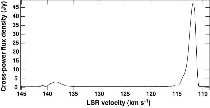
Figure 1: Cross-power spectrum of the OH masers in IRAS 18460$-$0151 obtained from the Effelsberg–Westerbork baseline.

The OH masers show a double-peaked spectrum with a velocity separation of $\approx$25 km s^-1($V_{\mbox{\scriptsize LSR}}$$=$111–114 and 136–140 km s^-1 in the phase-referencing-based cube and $V_{\mbox{\scriptsize LSR}}$$=$111–116 and 139–140 km s^-1 in the self-calibration-based cube), which is typical of that seen in other AGB stars. Figure 1 shows the cross-power spectrum of the OH masers in I18460. Table 5 gives the parameters of the OH maser spots detected using the two types of calibration scheme. The reason for the difference in the velocity ranges in which the maser spots are detected is unclear, but we speculate is due to the difference in the dynamic range caused by different conditions in phase calibration and the difference in the synthesized beam patterns. They are also exactly associated with the central H₂O maser components (see Section 3.4).

3.1 The Collimated Fast Jet

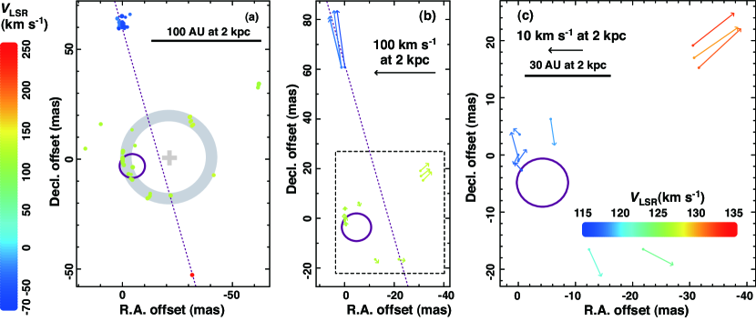
Figure 2: H₂O masers found in IRAS 18460$-$0151 in 2006–2007. (a) All of the H₂O maser features (dots) detected in all observations. The three-epoch maps are superposed using the common phase-reference maser spot in the maser feature IRAS 18460$-$0151:I2013-6 located at the map origin. A dashed magenta line (shown also in (b)) indicates the axis of the fast jet. A thick gray circle indicates a maser feature ring whose center is marked with a grey plus sign. An opened magenta ellipse (also shown in sub-panels (b) and (c)) indicates the location of the dynamical center of the central spherical flow, which was estimated by model fitting and whose uncertainty is indicated by the size of the ellipse. (b) Relative proper motions of H₂O masers (arrows) in the whole region of IRAS 18460$-$0151, which were measured with respect to the position-reference maser feature IRAS 18460$-$0151:I2013 -6. (c) Same as (b) but in the central region shown in a dashed box in (b). The systemic motion ($-$1.4, 2.4)(km s^-1) has been subtracted from the originally measured proper motions.

Figure 2 shows a comprehensive view of the spatiokinematics of H₂O masers in I18460 found in the first three epochs. As shown in Figure 2(a) and (b), the blue-shifted ($-68$ km s^-1$\lesssim$ $V_{\mbox{\scriptsize LSR}}$$\lesssim-17$ km s^-1) and red-shifted ($V_{\mbox{\scriptsize LSR}}$$\simeq$242 km s^-1) components are separated by $\approx$120 mas, corresponding to a linear scale of $\approx$240 AU at 2 kpc. We detected highly collimated, fast proper motions of the blue-shifted masers ($\mu\approx$10 mas yr^-1) with respect to the central masers. However, we could not measure proper motions of the red-shifted masers because they were detected at only the first epoch. Nevertheless we can approximate the relative proper motions of the blue-shifted masers with respect to the central masers as the velocity vectors of one side of the bipolar jet components. The maser locations and motions projected on the sky give a dynamical age of the jet to be only $\approx$6 yr in the observation epochs of 2006 September–2007 February.

The proper motions are well aligned along the jet axis, which is defined here to be a straight line connecting the blue-shifted masers with the red-shifted. The jet axis passes through the central masers. If we assume a circular distribution of the central masers (a thick grey circle in Figure 2(a) ), the separation between the circle center (a plus symbol in Figure 2(a) ) and the jet axis is only $\approx$10 mas ($\approx$20 AU). Because of the limited number of jet masers, this paper does not discuss a precessing jet model as proposed by Imai et al. (2005) and Yung et al. (2011).

The center velocity of the two velocity components of the jet masers ranges between $V_{\rm center}\approx$87–113 km s^-1, depending on which pair of the blue-shifted and red-shifted components are linked. Pairing of the $V_{\mbox{\scriptsize LSR}}$$\simeq$242 and $-17$ km s^-1 components gives $V_{\rm center}\approx$113 km s^-1, which is close to the systemic velocities derived from the central components and the OH masers ($V_{\mbox{\scriptsize LSR}}$$\sim$125 km s^-1) as mentioned in Sections 3.2 and 3.4, respectively. However, we cannot rule out pairing the $V_{\mbox{\scriptsize LSR}}$$\simeq$242 and $-67$ km s^-1 components to derive the center velocity. We derive a three-dimensional flow speed of $V_{\rm jet}\approx$180 km s^-1 at an inclination of $i\approx$32° with respect to the line of sight under the assumption of $V_{\rm sys}\approx$87 km s^-1İf we assume $V_{\rm sys}\approx$125 km s^-1, then we derive $V_{\rm jet}\approx$150 km s^-1 at $i\approx$40°Ṫhe implication of the difference in the assumed systemic velocity is discussed in Section 4.2. In both cases, a position angle of the jet, P.A.$\approx$8° east from north, is derived.

3.2 The Central Slow Flow Traced by H₂O Masers

As briefly mentioned in Section 3.1 and as shown in Figure 2(a), the distribution of a large fraction of H₂O maser features in the central component is well expressed by a (thick) ring with a radius of $\approx$18 mas ($\approx$36 AU). The maser features located in the central region but outside the ring are distributed in the east–west direction, perpendicular to the jet axis. We are able to measure 11 relative proper motions of H₂O masers. As shown in Figure 2(b) and (c), the proper motions are also loosely collimated perpendicular to the jet axis and exhibit an expanding flow.

In order to derive the kinematical parameters of this central outflow, we undertook a least-squares method based model-fitting analysis as described by Imai  et al. (2000) and Imai et al. (2012b). Using the model fitting, we derive a position vector of the originating point of outflow in the maser map, $(\Delta X_{\rm 0},\Delta Y_{\rm 0})$ and a velocity vector of the originating point, $(V_{0x},V_{0y})$. They were estimated by minimizing a $\chi^{2}$ value,

$$\chi^{2} = \frac{1}{3N_{\rm m}-N_{\rm p}}\sum^{N_{\rm m}}_{i}\left\{\frac{\left[\mu_{ix}-w_{ix}/(a_{{\rm 0}}D)\right]^{2}}{\sigma^{2}_{\mu_{ix}}}\right.$$ (1)

$$\left.+\frac{\left[\mu_{iy}-w_{iy}/(a_{{\rm 0}}D)\right]^{2}}{\sigma^{2}_{\mu_{iy}}}+\frac{\left[u_{iz}-w_{iz}\right]^{2}}{\sigma^{2}_{u_{iz}}}\right\}.$$

Here $N_{\rm m}=11$ is the number of maser features with measured proper motions, $N_{\rm p}=4$ the number of free parameters in the model fitting, $a_{\rm 0}=$4.74 km s^-1 mas^-1yr kpc^-1 a conversion factor from a proper motion to a transverse velocity, and $D\equiv$2.0 kpc the distance to the maser source from the Sun as determined below. $\mu_{ix}$ and $\mu_{iy}$ are the observed proper motion components in the R.A. and decl. directions, respectively, $\sigma_{\mu_{ix}}$ and $\sigma_{\mu_{iy}}$ their uncertainties; $u_{iz}$ the observed LSR velocity, and $\sigma_{iz}$ its uncertainty. For simplicity we assume a radially expanding outflow. In this case, the modeled velocity vector, $w_{i}$ $(w_{ix},w_{iy},w_{iz})$, is given as

$$\mbox{\boldmath$w_{i}$}=\mbox{\boldmath$V_{\rm 0}$}(V_{{\rm 0}x},V_{{\rm 0}y},V_{{\rm 0}z})+V_{\rm exp}(i)\frac{\mbox{\boldmath$r_{i}$}}{r_{i}},\\$$ (2)

where

$$r_{i} = \mbox{\boldmath$x_{i}$}(x_{i},y_{i},z_{i})-\mbox{\boldmath$x_{\rm 0}$}(\Delta X_{\rm 0},\Delta Y_{\rm 0}),$$ (3)

$$z_{i} = \frac{(u_{iz}-V_{{\rm 0}z})(r^{2}_{ix}+r^{2}_{iy})}{(u_{ix}-V_{{\rm 0}x})r_{ix}+(u_{iy}-V_{{\rm 0}y})r_{iy}},$$ (4)

$$u_{ix} = \mu_{ix}a_{\rm 0}D,\;\;u_{iy}=\mu_{iy}a_{\rm 0}D.$$ (5)

Table 6 gives the parameters derived through fitting. A magenta ellipse in Figure 2(a)–(c) indicates the estimated location of the originating point of the outflow; its size indicates the uncertainty of the location. The location appears biased to the eastern maser feature cluster due to the biased maser distribution and the complicated maser motions of the eastern cluster. The radial expansion velocities of the individual features are calculated after the model fitting using the following equation (Equation 7 of Imai et al. 2011)

$$V_{\rm exp}(i)=\frac{(u_{ix}-V_{{\rm 0}x})r_{ix}+(u_{iy}-V_{{\rm 0}y})r_{iy}+(u_{iz}-V_{{\rm 0}z})r_{iz}}{r_{i}}.$$ (6)

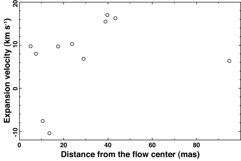
Figure 3: Distribution of the expansion velocities of the individual H₂O maser features in the central region of IRAS 18460$-$0151, which are derived from the fitting to a radially expanding flow model.

Figure 3 shows the distribution of the expansion velocities. The data points seem to concentrate around an expansion velocity of $\approx$9 km s^-1 near the outflow origin and $\sim$17 km s^-1 at the outer region. It is difficult, however, to recognize such outward acceleration from the limited number of data points. These values are typical of those seen in other AGB CSEs.

One can estimate the distance to I18460 using the statistical parallax method. This method assumes a uniform and random velocity field of gas clumps, therefore a velocity variance on the plane of the sky is expected to be equal to that in the line of sight. The equality of transverse and line-of-sight (or radial) velocity variances is also applicable to a spherically expanding model, such as the case of I18460. From the variances of proper motions and radial velocities of maser features, $\sigma^{2}_{\mu}$ and $\sigma^{2}_{v}$, respectively, the source distance and its uncertainty, $D$ and $\sigma_{D}$ respectively, are estimated using the following equations (Schneps et al., 1981):

$$D=\sigma_{v}/\sigma_{\mu},\;\;\;\frac{\sigma_{D}}{D}\sim\left\{\frac{1}{2N_{m}}+\frac{1}{4N_{m}}\left[1-\left(\frac{\epsilon_{\rm obs}}{\sigma^{\rm obs}_{\mu}}\right)^{2}\right]^{-1}\right\}^{1/2}.$$ (7)

We calculated a radial velocity variance, including a contribution from the expanding flow, $\sigma^{2}_{v_{z}}=$40.38 (km s^-1)² from a mean square deviation from the systemic velocity. The obtained proper motion variance was corrected for its error, $\epsilon^{2}_{\rm obs}$, by the following equation

$$\sigma^{2}_{\mu}=(\sigma^{\rm obs}_{\mu})^{2}-\epsilon^{2}_{\rm obs}.$$ (8)

We obtained the corrected variances of proper motions, $(\sigma_{\mu_{x}},\sigma_{\mu_{y}})=(0.61,0.63)$ in units of mas yr^-1. Their errors, (0.38, 0.39) (mas yr^-1), were derived from the uncertainties of the measured proper motions. These values give statistical parallax distance values: 2.2$\pm$0.6 kpc (between $\sigma_{\mu_{x}}$ and $\sigma_{v_{z}}$) and 2.1$\pm$0.6 kpc (between $\sigma_{\mu_{y}}$ and $\sigma_{v_{z}}$), yielding a weighted mean value of $D=2.1\pm 0.6$ kpc. The justification of the derived distance is discussed in Section 4.1.

3.3 The Stellar Secular Motion

We obtained five absolute proper motions of H₂O maser features observed in 2008–2009. Because of intrinsic fading of the H₂O masers, we detect the central component with a smaller number of features than that in 2006–2007. The northeast–southwest alignment and the proper motions of the H₂O maser features found in 2008–2009 were similar to those found in 2006–2007 (Figure 2(c) ). Therefore, we can assume that the masers from the different epochs are likely associated with a common origin. Two out of the five maser features were detected in all three epochs in 2008–2009. We fitted their absolute motions with respect to the position-reference source J1851 to the modeled motions, each of which was assumed to be composed of a constant velocity motion and an annual parallactic motion ($N_{\rm p}=5$).

Table 7 shows the results of the maser motion fitting. We obtained annual parallax values of 0.45–0.58 mas, corresponding to a range of the distance to I18460 of 1.7–2.2 kpc. However, the time baseline was too short (only 5 months) and the degree of freedom in the model fitting was too low ($2N_{\rm e}-N_{\rm p}=1$ where $N_{\rm e}=3$ is the number of observing epochs) for reliable analysis. Therefore, the derived parallax was used just to extract the non-negligible parallax modulations and to obtain more precise linear proper motions required for further analysis. Thus we derived the absolute proper motion of the position-reference maser feature (IRAS 18460$-$0151:I2013-19) of $(\mu_{\rm X},\mu_{\rm Y})=(-3.73\pm 1.17,-6.61\pm 0.41)$ mas in the celestial coordinates.

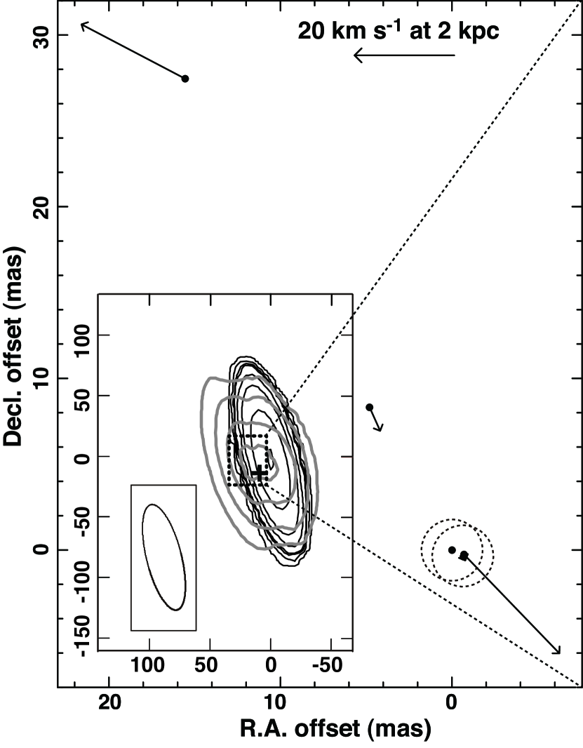
Figure 4: H₂O and OH masers observed in 2008 September–2009 February and in 2007 June, respectively. Here the self-calibration based map of the OH masers is displayed. The relative positions and proper motions of H₂O masers (filled circles and arrows, respectively) were measured with respect to the position-reference maser feature IRAS 18460$-$0151:I2013-19. The location of the two features IRAS 18460$-$0151:I2013-18 and 19, whose absolute motions were measured, are indicated by the centers of the dotted circles. The left-bottom sub-panel shows the velocity-integrated brightness distribution of the OH masers in the blue-shifted (black contours, $V_{\mbox{\scriptsize LSR}}$$=$111.0–115.6 km s^-1) and the red-shifted (gray contours, $V_{\mbox{\scriptsize LSR}}$$=$138.6–140.1 km s^-1) components, respectively. The contour levels are 0.18, 0.72, 1.44, 1.98, 5.76, 11.52, 23.04, and 39.60 Jy beam^-1km s^-1. The coordinate offsets are given with respect to the $V_{\mbox{\scriptsize LSR}}$$=$111.7 km s^-1 component of the OH masers. The ellipse at the left-bottom corner of this sub-panel shows the synthesized beam pattern. The plus symbol indicates the location of the H₂O maser feature IRAS 18460$-$0151:I2013-19 in this coordinate system.

Figure 4 shows the relative proper motions of the H₂O maser features found in 2008–2009 with respect to the position-reference feature. They exhibit expanding flow motions, similar to the masers shown in Figures 2(b)–(c) . This is clear even if we eliminate the motion of the feature, IRAS 18460$-$0151:I2013-17, which was detected at only two epochs and whose measured large relative proper motion was doubtful. Using the proper motion data of the features IRAS 18460$-$0151:I2013- 16, 18, 19, and 20, we estimated the stellar motion to be $(\Delta_{\mu X}^{\ast},\Delta_{\mu Y}^{\ast})\approx(0.49,0.14)$(mas yr^-1) with respect to the position-reference feature. This corresponds to an expanding velocity of the CSE of $\approx$5 km s^-1. The uncertainty of the relative stellar motion may be comparable to or smaller than this value. We added, therefore, this stellar motion to both the absolute proper motion of the reference feature and its error to obtain a stellar secular motion, $(\mu_{\rm X},\mu_{\rm Y})=(-3.24\pm 1.27,-6.47\pm 0.43)$ mas. The absolute coordinates of the reference feature were determined to be $\alpha_{\rm J2000}=$18^h48^m43^s.02792$\pm$0^s.00006, $\delta_{\rm J2000}=$ $-$01^∘48^′30$\farcs$46141$\pm$0$\farcs$00019 in 2008 September.

3.4 The Circumstellar Envelope Traced by OH Masers

Figure 4 shows the velocity-integrated brightness contour map of the two velocity components of the OH masers obtained from the self-calibration-based image cube. The origin of the contour map is set to the position of the reference OH maser spot at $V_{\mbox{\scriptsize LSR}}$$=$111.7 km s^-1, whose absolute coordinates were determined on the phase-referencing based image cube to be $\alpha_{\rm J2000}=$18^h48^m43^s.02701$\pm$0^s.00007, $\delta_{\rm J2000}=$ $-$01^∘48^′30$\farcs$4526$\pm$0$\farcs$0026. Interestingly, the position-reference H₂O feature and OH spot were located within 10 mas (see Section 3.3), corresponding to a linear scale of $\approx$20 AU, even taking into account the maser positions at the different epochs and the maser motions in the period of these epochs. The OH masers and the central H₂O ones have a common LSR velocity range (110–140 km s^-1) and indicate similar expansion velocities (10–20 km s^-1, Section 3.2). It is strongly suggested that these masers share a common origin.

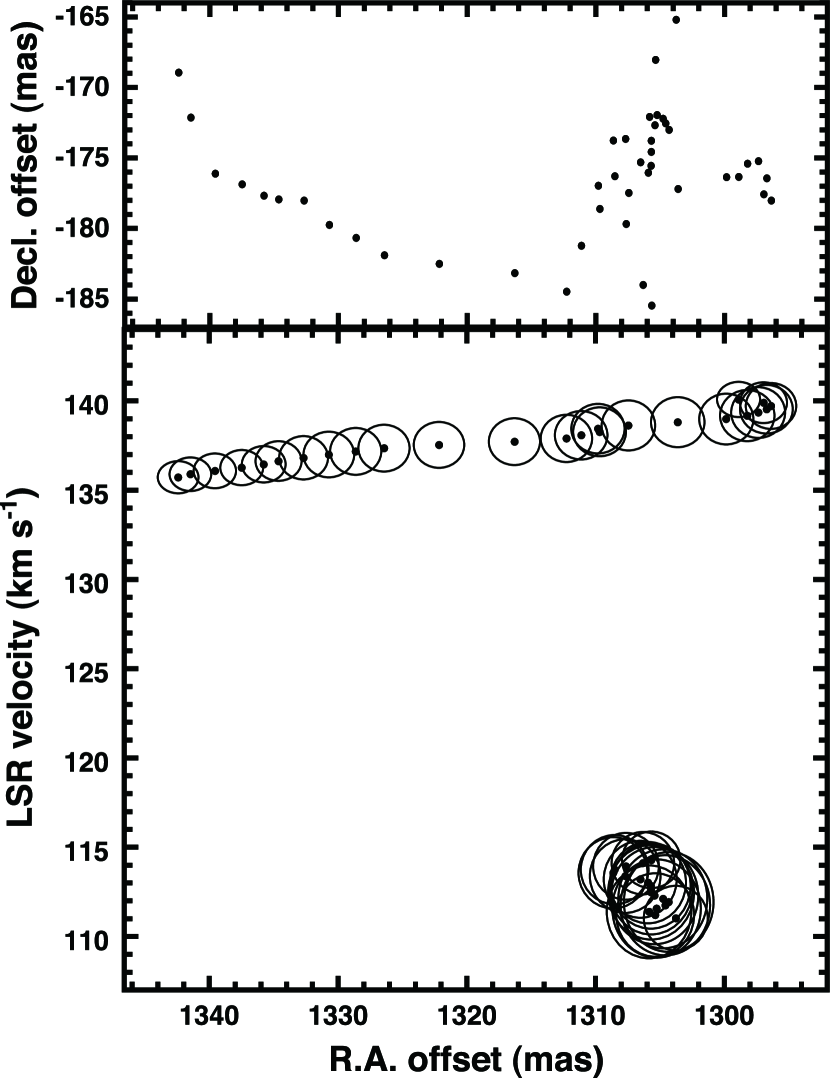
Figure 5: Angular distribution and position–velocity diagrams of the OH masers IRAS 18460$-$0151, which were detected on the phase-referencing-based image cube, denoted by filled circles. The size of the circle around the maser in the position–velocity diagram is proportional to logarithmic scale of its intensity.

Figure 5 shows the distribution of the OH masers in more detail. Each of the maser spots was resolved out on baselines to the Hartebeesthoek station: the spot size was estimated to be $\gtrsim$25 mas. The blue-shifted and red-shifted clusters of OH maser spots were split into the east–west direction by a separation of $\approx$50 mas, comparable to the extent of the central component of H₂O masers. The origin of a systematic LSR velocity gradient visible in only the red-shifted component is unknown and it should be investigated whether this velocity gradient is always visible. But we note that the directions of the elongation of the H₂O maser distribution (Section 3.2), the cluster splitting, and the velocity gradient are perpendicular to the axis of the H₂O maser jet (Section 3.1). Furthermore, the expansion speeds and the angular distribution sizes are equal for the central component of H₂O masers and the OH masers. These properties are similar to those of H₂O and OH masers in W 43A (Imai et al., 2002; Imai, 2007; Imai et al., 2008), where the existence of H₂O masers that are not associated with the collimated jet was first claimed. However, the kinematics of the W43A H₂O masers looks different from that of the OH maser although the kinematic information was quite limited in that source. The central component of H₂O masers in I18460 is the first example whose spatiokinematical structure was determined through the construction of the radially expanding flow model as described in Section 3.2 and compared with the kinematics of the OH masers.

4 DISCUSSION

4.1 Distance to IRAS 18460$-$0151

The results of this paper favor a much shorter distance to I18460 ($D\sim$2.0 kpc) than the derived kinematic distance ($D_{\rm kin}\sim$6.9 kpc). The latter value is obtained when one uses only the radial velocity and assumes a circular orbit of I18460 in the Milky Way. This suggests that this source is located close to a tangential point in the Milky Way. Using both the radial velocity and the proper motion (Section 3.3), $D_{\rm kin}\sim$6.0 or 7.8 kpc is obtained. However, unless the maser source is of a young generation, the assumption of a circular orbit is unlikely (see also Section 4.4).

As described in Section 3.2, the statistical parallax distance to I18460 is estimated as $D_{\rm stat}=2.1\pm 0.6$ kpc. As shown in Figure 2, the distribution of the central components of H₂O masers is elongated in the east–west direction. In addition, as shown in Figure 3, the expanding flow appears to be accelerated outward. These results may affect this estimate of distance; the variance of proper motions may have a bias in the east–west direction. In practice, as already mentioned, the outward acceleration is negligible and the calculated results support that such a variance bias is also negligible. On the other hand, if these H₂O masers are associated with a face-on equatorial flow, then a transverse velocity variance larger than that in the radial direction is expected, causing a possible bias to a shorter distance. This possibility is also unlikely when taking into account the similarity of the kinematics of the H₂O masers to that of the 1612 MHz OH masers, which suggest spherical expansion. Thus, even the possible bias in $D_{\rm stat}$ cannot explain the much shorter distance to I18460. The annual parallax unambiguously rules out a large $D_{\rm kin}$, although the uncertainty of the parallax is very large.

4.2 The Collimated Jet in IRAS 18460$-$0151

The driving mechanism of the WF jet is still in debate, but a comparison of the jet parameters with other parameters of the WF sources will shed light on the mechanism. For those WFs with an estimated three-dimensional jet velocity, however, we find so far no clear correlation among the three-dimensional velocity, dynamical age, and degree of collimation of the jet and the stellar luminosity (roughly evaluated with the IRAS flux at the 25 $\mu$m band multiplied by the square of the source distance).

An offset of the center velocity of a collimated jet from the systemic velocity of a CSE and an angular offset of the originating point of a collimated jet from that of a CSE are observable in the maser spatiokinematics. The existence of these offsets implies the existence of a binary system in which the jet and the CSE originate from different host stars. In the case of I18460, as shown in Figures 2 and 4 (see Sections 3.1, 3.2, and 3.4), an upper limit to the angular offset mentioned above was given to be $\lesssim$20 mas ($\lesssim$40 AU at 2 kpc). The center velocity offset was derived to be 10–40 km s^-1 from the center velocity of the jet H₂O masers and the systemic velocity derived from the OH maser spectrum (see Section 3.1). The derived velocity offset is roughly consistent with those in IRAS 16342$-$3814 and IRAS 18286$-$0959, in which the center velocities of H₂O and OH masers differ by up to 30 km s^-1(Claussen et al. 2009; Yung et al. 2011; Imai et al. 2013a, hereafter Paper I). However, uncertainties of these center velocities of the jet masers are large. Unless the point symmetry of the H₂O maser spectra is well examined, the large uncertainty of the center velocity of the jet cannot be reduced, so it prevents us from any realistic constraint on the orbital parameters of a supposed binary system or being convinced of the existence of the binary system.

Here, we consider the possibility of identification of a binary system, with one component driving the WF jet while the other hosts the CSE. The latter may be an O-rich intermediate-mass AGB or post-AGB star (Imai  et al., 2012a), so here we assume a current stellar mass of $\sim$1 $M_{\sun}$. In the case of W 43A, in which the center velocities of the H₂O, OH, and SiO masers are estimated to be consistent with one another within a few  km s^-1, it is possible to consider a separation of 100 AU between two stars, which is comparable to the upper limit to the separation estimated from the maser observations (Imai et al. 2002, 2005, see also the case of OH 12.8$-$0.9, Boboltz & Marvel 2007). If a companion orbits the supposed star with a velocity of 10–40 km s^-1 as estimated in I18460, the separation of these stars may be in a range of 0.6–9 AU, which cannot be spatially resolved with the current analysis technique relying on the maser data. On the other hand, the case of the highest velocity offset corresponds to a velocity fluctuation of the host star of $\gtrsim$0.3 km s^-1 at 9 AU and an orbital period of $\lesssim$30 yr. These derived parameters will be examined in future infrared and sub-millimeter observations which can resolve such a scale and which will enable us to conduct high-resolution spectroscopy of molecular lines associated with the central stars and the accompanying jets and CSEs. In any case, finding point a symmetric distribution of the jet masers and a reasonable jet model may be necessary to more precisely estimate the center velocity of the jet, which is essential to identify a binary system.

It is noteworthy that the H₂O masers in I18460 had faded between the 2006–2007 and 2008–2009 seasons. It should be taken into account that stellar H₂O masers are highly variable in both their angular and velocity distribution and some of the variation will be correlated with stellar pulsation (e.g., Bowers & Johnston 1994). In the case of the WF jet masers, however, it is possible that we are observing the evolution of the jet on a timescale comparable to the estimated dynamical time scale (see Section 3.1). We have to confirm, using future long-term observations, whether we are observing the true “death” of a WF or recurrent jet ejections; this should reveal the role of the WF jet in shaping the future planetary nebula.

4.3 The Relic AGB CSE in IRAS 18460$-$0151

The AGB CSE/equatorial flow as well as the collimated fast jet is important components to probe the evolutionary status of the WF source. As mentioned in Section 3.4, the OH masers and the central component of H₂O masers in I18460 resemble those of AGB CSEs. Taking into account that these masers do not have a high expansion velocity ($V_{\rm exp}\approx$8–15 km s^-1) and they trace only a limited volume of the CSE or equatorial flow, these masers likely have close association with each other as shown in some OH/IR stars.

It is noteworthy that the equatorial elongation in the H₂O/OH CSE is still marginal. It is suggested that the 1612 MHz OH masers are radially amplified and it is possible that their area projected on the plane of sky is sometimes smaller than that of H₂O masers. Even taking into account these factors, the noted properties of the OH and H₂O masers in I18460 imply that this CSE may be a relic AGB CSE rather than a product of recent rapid growth of an equatorial torus or flow as suggested by Huggins (2007). Because the collimated jet of I18460 still looks extremely young (it has a dynamical age of only $\sim$6 yr, see Section 3.1) it is too early to observe the intrinsic evolution of the equatorial flow even if it is recently launched. Huggins (2007) suggested a time lag of a few hundred years between the rapid growth of the equatorial torus and the ignition of the collimated jet. In practice, the dynamical age of the I18460 CSE is only $\approx$140 yr. Any dynamical age derived from the data of H₂O and OH masers may be much shorter than the true age of the dynamical component (i.e., jet or CSE). Nevertheless we believe that the former time scale is meaningful when comparing the dynamical time scales among the maser sources when discussing the evolution of the maser sources. In fact, Imai et al. (2005) and Boboltz & Marvel (2005) have found the temporal evolution of the H₂O maser jets in W 43A and OH 12.8$-$0.9 on the decade scale, respectively. In both cases, the expansion rate of the H₂O maser region in the jet is roughly consistent with that expected from the dynamical ages.

It is unclear whether the existence of the relic AGB CSE indicates that its hosting source is in the early phase of the WF. As already mentioned, the dynamical ages of the CSEs are much longer than those of the jets. The jet will affect only the inner part of the CSE in the WF phase, and the volume of the interaction with the highly collimated jet will be still quite limited. Therefore, it is difficult to find any correlation between the kinematic parameters of the jet and the CSE with the overall properties of the CSE as traced by its infrared colors. However, if we suppose a beaming effect of H₂O and OH masers, the small interaction with the jet may enhance the difference in preferred locations of these masers in the CSE. Similar to 1612 MHz OH masers, H₂O masers in a CSE prefer radial beaming, in which the maser emission is amplified radially with respect to the central star (e.g., Takaba et al. 1994). In this case, one can see H₂O masers associated with the CSE if the collimated jet breaks up the CSE only along the plane of the sky while THE CSE is still maintained in the line of sight. After checking the previous VLBI observations of WFs (Imai et al., 2002; Boboltz & Marvel, 2007; Claussen et al., 2009; Day et al., 2010; Yung et al., 2011), we speculate that the central H₂O masers of the WFs, associated with relic AGB CSEs, may be visible in the case in which the jet inclination angle with respect to the line of sight is sufficiently large ($i>$30°). This speculation should be further examined in future VLBI observations of other WFs.

4.4 The Secular Motion of IRAS 18460$-$0151

As shown in Sections 3.2 and 3.3, we have derived the distance and the secular motion of I18460 to be $D=2.1\pm 0.6$ kpc and $(\mu_{\rm X},\mu_{\rm Y})=(-3.24\pm 1.27,-6.47\pm 0.43)$ mas, respectively. Based on these values, we further estimate the location and the three-dimensional motion of I18460 in the Milky Way. Table 8 gives the list of relevant parameters. We note common properties of the WFs whose kinematics in the Milky Way have been estimated (IRAS 19134$+$2131, Imai  et al. 2007; IRAS 18286$-$0959, Paper I). Although some of the WFs are located several hundred parsecs away from the Galactic mid-plane (IRAS 163424$-$3814, IRAS 19134$+$2131), a large fraction of the WFs is located in the Galactic thin disk as seen for massive-star forming regions. Nevertheless, their three-dimensional motions have large deviations by $\gtrsim$50 km s^-1 from those expected from the circular Galactic rotation. It is expected that the motions of the WF sources have such large deviation as a result of dynamical relaxation during their relatively long lifetimes ($>10^{7}$ yr). However, this is inconsistent with the observation that some of the WFs, including I18460, still persist in the Galactic mid-plane. Paper I point out the possibility of a binary motion for such a peculiar motion.

5 CONCLUSIONS

The present VLBA and EVN observations have revealed the spatiokinematical structures of both of the collimated fast jet and the slowly expanding equatorial flow or CSE associated with I18460. The dynamical ages of these kinematical components are extremely short ($\sim$6 and $\sim$140 yr, respectively) although these values may not be equal to their true ages. The suggestion that I18460 should be in a very young stage of the WF evolution is supported by its association with the CSE as seen in OH/IR stars. The driving sources of the different components are located within $\sim$10 mas ($\sim$20 AU), a situation very similar to the case of the H₂O and SiO masers in W 43A (Imai et al., 2005). By adding the present results, the common properties of the three-dimensional velocity vectors of the WFs in the Milky Way have been elucidated, which implies that the WFs harbor binary systems. Future observations that enable us to resolve such binary systems ($\lesssim$20 AU at a few kilo parsecs), as those conducted with new facilities such as the Atacama Large Millimeter-submillimeter Array (ALMA), will directly shed light on the evolution of AGB/post-AGB stars generating the WFs.

Table 1: Parameters of the VLBA Observations and Data Reduction for Individual Epochs

Observation	Epoch	$V_{\mbox{\scriptsize ref}}$	Noise	Dynamic	Beam
code	(yy/mm/dd)	(km s-1)	(mJy beam-1)	Range	(mas)	$N_{\mbox{\scriptsize f}}$
BI033A	06/09/15	117.7	2.6	$\sim$90	1.31$\times$0.88, 2∘.7	34
BI033B	06/11/09	117.6	3.1	$\sim$220	1.37$\times$0.96, 17∘.4	27
BI033C	07/02/03	118.3	1.9	$\sim$110	1.50$\times$0.96, $-$12∘.7	16
BI036A	08/09/05	—	12	$\sim$30	1.77$\times$1.18, 11∘.1	11
BI036B	08/11/18	—	11	$\sim$50	1.65$\times$0.92, $-$2∘.1	10
BI036C	09/02/06	—	9.7	$\sim$40	1.58$\times$0.95, $-$3∘.5	3

Table 2: Parameters of the Detected H₂O Maser Features Found in 2006–2007

$V_{\mbox{\tiny LSR}}$	R.A. Offset		Decl. Offset		$I$	$\Delta V$
(km s-1)	(mas)		(mas)		(Jy beam-1)	(km s-1)
2006 September 15
$241.79$	$-31.66$ $\pm$	$0.02$	$-52.66$ $\pm$	$0.06$	$0.03$	$0.84$
$132.14$	$-31.60$ $\pm$	$0.02$	$15.24$ $\pm$	$0.04$	$0.07$	$0.84$
$130.56$	$-30.76$ $\pm$	$0.02$	$16.96$ $\pm$	$0.02$	$0.09$	$0.84$
$123.43$	$-21.86$ $\pm$	$0.02$	$-16.52$ $\pm$	$0.02$	$0.15$	$1.05$
$121.26$	$-12.40$ $\pm$	$0.01$	$-16.56$ $\pm$	$0.02$	$0.36$	$0.63$
$121.26$	$-12.59$ $\pm$	$0.02$	$-15.66$ $\pm$	$0.01$	$0.06$	$0.21$
$121.26$	$-12.15$ $\pm$	$0.01$	$-17.44$ $\pm$	$0.01$	$0.09$	$0.21$
$118.95$	$-3.94$ $\pm$	$0.03$	$-6.99$ $\pm$	$0.05$	$0.31$	$0.63$
$118.87$	$-5.68$ $\pm$	$0.02$	$6.25$ $\pm$	$0.06$	$0.43$	$0.84$
$118.37$	$-0.26$ $\pm$	$0.02$	$3.57$ $\pm$	$0.02$	$2.39$	$1.89$
$119.16$	$-4.34$ $\pm$	$0.11$	$13.37$ $\pm$	$0.08$	$0.19$	$0.84$
$118.74$	$-4.67$ $\pm$	$0.02$	$-3.71$ $\pm$	$0.04$	$0.35$	$0.21$
$118.10$	$-0.11$ $\pm$	$0.01$	$-0.85$ $\pm$	$0.05$	$1.54$	$0.63$
$117.85$	$-0.01$ $\pm$	$0.02$	$-0.01$ $\pm$	$0.05$	$2.66$	$1.90$
$117.89$	$-0.01$ $\pm$	$0.05$	$-1.08$ $\pm$	$0.05$	$0.90$	$0.84$
$116.94$	$-0.61$ $\pm$	$0.01$	$-2.70$ $\pm$	$0.04$	$0.09$	$0.84$
$113.54$	$-61.82$ $\pm$	$0.03$	$33.49$ $\pm$	$0.03$	$0.07$	$1.47$
$113.68$	$-61.59$ $\pm$	$0.01$	$32.56$ $\pm$	$0.01$	$0.06$	$0.42$
$113.47$	$-62.01$ $\pm$	$0.01$	$34.34$ $\pm$	$0.01$	$0.12$	$0.21$
$-17.11$	$1.24$ $\pm$	$0.05$	$60.68$ $\pm$	$0.09$	$0.04$	$1.26$
$-17.49$	$1.22$ $\pm$	$0.11$	$60.73$ $\pm$	$0.18$	$0.13$	$0.84$
$-19.52$	$1.24$ $\pm$	$0.02$	$60.74$ $\pm$	$0.06$	$0.12$	$2.32$
$-17.82$	$1.79$ $\pm$	$0.05$	$59.66$ $\pm$	$0.10$	$0.04$	$1.47$
$-19.71$	$1.21$ $\pm$	$0.02$	$60.80$ $\pm$	$0.03$	$0.13$	$0.63$
$-22.96$	$-3.40$ $\pm$	$0.03$	$65.86$ $\pm$	$0.06$	$0.04$	$0.21$
$-43.20$	$-2.21$ $\pm$	$0.04$	$60.06$ $\pm$	$0.11$	$0.04$	$0.84$
$-47.56$	$-1.09$ $\pm$	$0.01$	$60.41$ $\pm$	$0.02$	$0.40$	$3.16$
$-46.99$	$-0.86$ $\pm$	$0.01$	$59.46$ $\pm$	$0.01$	$0.11$	$1.26$
$-49.15$	$-0.14$ $\pm$	$0.01$	$60.82$ $\pm$	$0.01$	$1.38$	$2.32$
$-49.22$	$0.09$ $\pm$	$0.01$	$59.86$ $\pm$	$0.01$	$0.27$	$0.84$
$-49.31$	$-0.30$ $\pm$	$0.02$	$61.73$ $\pm$	$0.01$	$0.17$	$0.21$
$-50.65$	$-1.32$ $\pm$	$0.01$	$60.22$ $\pm$	$0.02$	$0.24$	$1.68$
$-54.21$	$0.12$ $\pm$	$0.02$	$60.74$ $\pm$	$0.06$	$0.08$	$2.11$
$-67.38$	$1.64$ $\pm$	$0.01$	$59.34$ $\pm$	$0.03$	$0.18$	$1.05$
2006 November 9
$133.06$	$-30.57$ $\pm$	$0.02$	$19.09$ $\pm$	$0.05$	$0.03$	$0.42$
$132.08$	$-31.84$ $\pm$	$0.02$	$15.37$ $\pm$	$0.02$	$0.11$	$1.26$
$130.52$	$-30.99$ $\pm$	$0.01$	$17.08$ $\pm$	$0.01$	$0.15$	$1.05$
$130.96$	$-41.48$ $\pm$	$0.02$	$-7.30$ $\pm$	$0.05$	$0.03$	$0.11$
$123.49$	$-22.03$ $\pm$	$0.01$	$-16.59$ $\pm$	$0.02$	$0.13$	$0.84$
$121.26$	$16.93$ $\pm$	$0.02$	$4.74$ $\pm$	$0.03$	$0.08$	$0.63$
$121.26$	$-12.48$ $\pm$	$0.01$	$-16.69$ $\pm$	$0.01$	$0.19$	$0.42$
$119.58$	$-4.45$ $\pm$	$0.03$	$-9.40$ $\pm$	$0.03$	$0.18$	$0.11$
$118.96$	$-5.72$ $\pm$	$0.02$	$6.12$ $\pm$	$0.05$	$0.91$	$1.05$
$118.34$	$-0.23$ $\pm$	$0.01$	$3.57$ $\pm$	$0.05$	$3.14$	$1.69$
$117.26$	$-0.21$ $\pm$	$0.01$	$3.23$ $\pm$	$0.04$	$0.14$	$0.42$
$118.26$	$-0.09$ $\pm$	$0.01$	$-0.71$ $\pm$	$0.06$	$2.08$	$0.63$
$118.02$	$-0.07$ $\pm$	$0.05$	$-1.03$ $\pm$	$0.10$	$0.70$	$1.05$
$118.32$	$-0.02$ $\pm$	$0.01$	$0.31$ $\pm$	$0.01$	$0.69$	$0.11$
$118.32$	$-0.05$ $\pm$	$0.01$	$2.66$ $\pm$	$0.01$	$0.64$	$0.42$
$118.10$	$0.04$ $\pm$	$0.01$	$-1.64$ $\pm$	$0.07$	$0.68$	$0.42$
$118.10$	$-0.03$ $\pm$	$0.01$	$-0.37$ $\pm$	$0.01$	$2.07$	$0.11$
$117.87$	$-0.01$ $\pm$	$0.02$	$-0.06$ $\pm$	$0.06$	$2.40$	$0.63$
$117.81$	$0.12$ $\pm$	$0.03$	$-0.84$ $\pm$	$0.01$	$1.07$	$1.26$
$117.89$	$-0.12$ $\pm$	$0.01$	$0.85$ $\pm$	$0.01$	$1.18$	$0.11$
$117.57$	$0.01$ $\pm$	$0.01$	$0.05$ $\pm$	$0.01$	$1.22$	$1.26$
$116.85$	$-0.59$ $\pm$	$0.01$	$-2.76$ $\pm$	$0.04$	$0.15$	$1.05$
$-17.74$	$1.54$ $\pm$	$0.02$	$62.05$ $\pm$	$0.03$	$0.13$	$1.90$
$-19.87$	$1.44$ $\pm$	$0.05$	$62.22$ $\pm$	$0.06$	$0.15$	$2.32$
$-21.07$	$1.39$ $\pm$	$0.03$	$62.23$ $\pm$	$0.05$	$0.09$	$1.48$
$-49.03$	$0.07$ $\pm$	$0.01$	$62.30$ $\pm$	$0.02$	$0.87$	$2.53$
$-48.89$	$0.24$ $\pm$	$0.02$	$61.36$ $\pm$	$0.04$	$0.10$	$1.05$
2007 February 3
$133.27$	$-30.64$ $\pm$	$0.02$	$15.65$ $\pm$	$0.10$	$0.02$	$0.63$
$132.05$	$-31.91$ $\pm$	$0.01$	$12.00$ $\pm$	$0.02$	$0.14$	$1.26$
$130.55$	$-31.08$ $\pm$	$0.02$	$13.64$ $\pm$	$0.01$	$0.10$	$1.05$
$124.06$	$-11.10$ $\pm$	$0.03$	$-21.62$ $\pm$	$0.04$	$0.03$	$0.63$
$120.42$	$10.11$ $\pm$	$0.04$	$12.15$ $\pm$	$0.07$	$0.03$	$0.11$
$118.40$	$0.04$ $\pm$	$0.01$	$-0.02$ $\pm$	$0.08$	$2.75$	$2.11$
$118.29$	$0.19$ $\pm$	$0.02$	$-4.20$ $\pm$	$0.09$	$1.25$	$0.63$
$117.89$	$-2.40$ $\pm$	$0.04$	$-10.55$ $\pm$	$0.07$	$0.07$	$0.11$
$117.89$	$0.26$ $\pm$	$0.01$	$-3.80$ $\pm$	$0.16$	$0.77$	$1.05$
$117.68$	$-3.36$ $\pm$	$0.04$	$-12.56$ $\pm$	$0.08$	$0.04$	$0.11$
$116.65$	$-0.31$ $\pm$	$0.02$	$-6.31$ $\pm$	$0.04$	$0.19$	$1.26$
$-15.81$	$2.66$ $\pm$	$0.11$	$60.17$ $\pm$	$0.07$	$0.63$	$6.32$
$-45.36$	$0.52$ $\pm$	$0.03$	$61.29$ $\pm$	$0.07$	$0.04$	$1.26$
$-47.01$	$0.50$ $\pm$	$0.02$	$61.29$ $\pm$	$0.04$	$0.06$	$1.48$
$-48.50$	$0.52$ $\pm$	$0.01$	$61.26$ $\pm$	$0.04$	$0.10$	$1.68$
$-46.57$	$-1.12$ $\pm$	$0.08$	$60.76$ $\pm$	$0.08$	$0.02$	$0.42$

Table 3: Same as Table 2 But in 2008–2009

$V_{\mbox{\tiny LSR}}$	R.A. offset		Decl. offset		$I$	$\Delta V$
(km s-1)	(mas)		(mas)		(Jy beam-1)	(km s-1)
2008 September 5
$121.47$	$39.52$ $\pm$	0.06	$20.92$ $\pm$	0.15	0.40	0.63
$121.47$	$36.48$ $\pm$	0.07	$0.72$ $\pm$	0.11	0.44	0.63
$121.47$	$36.86$ $\pm$	0.07	$24.97$ $\pm$	0.13	0.40	0.42
$121.04$	$29.36$ $\pm$	0.07	$13.39$ $\pm$	0.12	0.72	1.05
$118.96$	$13.82$ $\pm$	0.14	$-14.06$ $\pm$	0.19	1.02	1.05
$118.10$	$13.13$ $\pm$	0.10	$-14.46$ $\pm$	0.30	2.75	0.84
$118.74$	$13.63$ $\pm$	0.10	$-15.26$ $\pm$	0.07	0.66	0.84
$118.99$	$17.03$ $\pm$	0.09	$6.57$ $\pm$	0.14	0.52	0.63
$117.89$	$13.11$ $\pm$	0.13	$-14.33$ $\pm$	0.11	2.29	0.63
$117.26$	$21.62$ $\pm$	0.08	$14.57$ $\pm$	0.27	0.52	0.63
$117.05$	$18.62$ $\pm$	0.06	$-5.74$ $\pm$	0.11	0.54	0.42
2008 November 18
$122.53$	$-6.16$ $\pm$	0.06	$-23.63$ $\pm$	0.11	0.25	0.42
$121.12$	$29.37$ $\pm$	0.06	$11.56$ $\pm$	0.05	0.62	1.47
$119.13$	$13.38$ $\pm$	0.12	$-16.12$ $\pm$	0.09	3.30	1.69
$118.08$	$12.68$ $\pm$	0.08	$-16.41$ $\pm$	0.13	2.33	0.63
$119.16$	$13.41$ $\pm$	0.10	$6.95$ $\pm$	0.13	0.74	0.63
$119.37$	$11.62$ $\pm$	0.06	$-29.24$ $\pm$	0.08	0.47	0.42
$119.11$	$13.67$ $\pm$	0.11	$7.26$ $\pm$	0.16	0.74	0.84
$117.68$	$12.26$ $\pm$	0.16	$-16.82$ $\pm$	0.12	1.18	0.42
$117.00$	$18.14$ $\pm$	0.04	$-7.91$ $\pm$	0.13	0.81	1.05
$117.05$	$18.48$ $\pm$	0.06	$16.06$ $\pm$	0.11	0.62	0.84
2009 February 6
$119.26$	$13.15$ $\pm$	0.11	$-17.35$ $\pm$	0.05	4.78	1.69
$118.27$	$12.47$ $\pm$	0.41	$-17.76$ $\pm$	0.27	1.50	1.68
$118.74$	$13.89$ $\pm$	0.06	$-16.81$ $\pm$	0.04	1.06	0.42

Table 4: Parameters of H₂O Maser Features Measured Their Relative Proper Motions in 2006–2007 and 2008–2009

Maser Feature No.	Position Offset		Proper Motion				Radial Motion		Peak Intensity
	(mas)		( mas yr-1)				(km s-1)		(Jy beam-1)
(IRAS 18460$-$0151:
I2013	R.A.	Decl.	$\mu_{X}$	$\sigma\mu_{X}$	$\mu_{Y}$	$\sigma\mu_{Y}$	VZ	$\Delta$VZ
									06/09/15	06/11/09	07/02/03
1	$-0.13$	$60.84$	$1.37$	0.09	$9.92$	0.17	$-49.15$	2.42	1.38	0.87	$\ldots$
2	$1.22$	$60.82$	$2.03$	0.20	$8.38$	0.17	$-19.71$	2.81	0.13	0.09	0.63
3	$1.25$	$60.76$	$1.31$	0.32	$9.94$	0.55	$-19.52$	2.32	0.12	0.15	$\ldots$
4	$1.23$	$60.75$	$2.10$	0.73	$8.92$	1.22	$-17.49$	1.37	0.06	0.13	$\ldots$
5	$-0.60$	$-2.68$	$0.06$	0.06	$0.48$	0.13	$116.94$	1.05	0.09	0.15	0.19
6	$0.00$	$0.01$	$0.00$	0.06	$-0.04$	0.34	$117.85$	1.19	2.66	2.40	0.77
7	$0.00$	$-1.06$	$-0.40$	0.42	$0.61$	0.70	$117.89$	0.94	0.90	0.70	$\ldots$
8	$-0.10$	$-0.83$	$0.09$	0.06	$1.11$	0.26	$118.10$	0.63	1.54	2.08	1.25
9	$-0.25$	$3.59$	$0.04$	0.04	$0.43$	0.20	$118.37$	1.90	2.39	3.14	2.75
10	$-5.67$	$6.27$	$-0.27$	0.19	$-0.57$	0.51	$118.87$	0.94	0.43	0.91	$\ldots$
11	$-12.39$	$-16.54$	$-0.53$	0.05	$-0.59$	0.17	$121.26$	0.52	0.36	0.19	$\ldots$
12	$-21.85$	$-16.50$	$-1.09$	0.12	$-0.24$	0.19	$123.43$	0.94	0.15	0.13	$\ldots$
13	$-30.75$	$16.98$	$-1.53$	0.07	$1.21$	0.06	$130.56$	0.98	0.09	0.15	0.10
14	$-31.59$	$15.26$	$-1.47$	0.05	$1.48$	0.10	$132.14$	1.12	0.07	0.11	0.14
15	$-30.56$	$19.15$	$-1.44$	0.13	$1.27$	0.45	$133.06$	0.52	$\ldots$	0.03	0.02
									08/09/05	08/11/18	09/02/06
16	$4.80$	$8.32$	$-0.22$	0.35	$-0.50$	0.82	$117.05$	0.73	0.54	0.81	$\ldots$
17	$-0.71$	$-0.27$	$-2.02$	1.01	$-2.09$	0.78	$117.89$	0.52	2.29	1.18	$\ldots$
18	$-0.69$	$-0.40$	$-0.03$	0.55	$-0.08$	0.96	$118.10$	1.05	2.75	2.33	1.50
19	$0.00$	$0.00$	$0.00$	0.41	$0.00$	0.37	$118.96$	1.48	1.02	3.30	4.78
20	$15.54$	$27.45$	$2.20$	0.45	$1.15$	0.63	$121.04$	1.26	0.72	0.62	$\ldots$

Table 5: Parameters of the Detected OH Maser Spots

	On the Phase-referencing Based Image Cube					On Self-calibration Based Image Cube
$V_{\mbox{\scriptsize LSR}}$	R.A. offset		Decl. offset		$I_{\rm peak}$	R.A. offset		Decl. offset		$I_{\rm peak}$
(km s-1)	(mas)		(mas)		(Jy beam-1)	(mas)		(mas)		(Jy beam-1)
Red-shifted components
$140.07$	$1298.88$	1.04	$-176.34$	3.19	0.55	$-6.13$	0.53	$-3.31$	1.53	0.30
$139.89$	$1296.94$	1.11	$-177.57$	3.30	0.78	$-7.55$	0.45	$-3.12$	1.19	0.47
$139.71$	$1296.36$	1.10	$-178.02$	3.26	1.08	$-8.36$	0.47	$-2.94$	1.28	0.65
$139.53$	$1296.71$	0.98	$-176.43$	2.86	1.31	$-8.45$	0.31	$-2.94$	0.82	0.81
$139.34$	$1297.36$	0.94	$-175.21$	2.70	1.50	$-7.82$	0.27	$-1.99$	0.69	0.98
$139.16$	$1298.20$	0.83	$-175.40$	2.31	1.53	$-7.49$	0.14	$-1.62$	0.33	1.09
$138.98$	$1299.84$	0.81	$-176.35$	2.05	1.50	$-6.12$	0.14	$-2.17$	0.30	1.11
$138.80$	$1303.61$	0.89	$-177.21$	2.03	1.43	$-2.41$	0.24	$-2.16$	0.47	1.01
$138.62$	$1307.45$	1.02	$-177.49$	2.10	1.42	$1.95$	0.29	$-1.86$	0.55	1.00
$138.44$	$1309.80$	1.18	$-176.97$	2.18	1.39	…
$138.26$	$1309.68$	1.18	$-178.61$	1.98	1.32	…
$138.07$	$1311.11$	1.23	$-181.22$	2.09	1.29	…
$137.89$	$1312.25$	1.46	$-184.48$	2.38	1.17	…
$137.71$	$1316.30$	1.34	$-183.16$	2.32	1.15	…
$137.53$	$1322.16$	1.42	$-182.51$	2.83	1.08	…
$137.35$	$1326.43$	1.17	$-181.91$	2.91	1.13	…
$137.16$	$1328.64$	1.08	$-180.67$	2.91	1.16	…
$136.98$	$1330.71$	0.97	$-179.75$	2.73	1.08	…
$136.80$	$1332.68$	0.97	$-178.03$	2.72	0.93	…
$136.62$	$1334.63$	1.00	$-177.94$	2.78	0.73	…
$136.44$	$1335.78$	0.99	$-177.68$	2.75	0.59	…
$136.26$	$1337.49$	1.05	$-176.88$	3.02	0.55	…
$136.08$	$1339.58$	1.21	$-176.12$	3.58	0.52	…
$135.89$	$1341.47$	1.09	$-172.14$	3.21	0.49	…
$135.71$	$1342.42$	1.02	$-168.96$	2.96	0.45	…
Blue-shifted components
$115.56$	…					$1.29$	0.43	$-25.10$	1.17	0.39
$115.38$	…					$0.69$	0.26	$-29.94$	0.69	0.58
$115.19$	…					$0.94$	0.27	$-28.32$	0.71	0.75
$115.01$	…					$1.24$	0.14	$-27.34$	0.36	0.78
$114.83$	…					$2.21$	0.15	$-22.51$	0.35	0.67
$114.65$	…					$2.05$	0.19	$-17.93$	0.46	0.56
$114.47$	…					$1.55$	0.30	$-13.95$	0.81	0.69
$114.29$	$1305.66$	1.04	$-185.46$	3.20	2.19	$0.39$	0.37	$-14.45$	1.03	1.09
$114.11$	$1306.32$	1.10	$-184.00$	3.36	3.18	$0.34$	0.35	$-13.84$	0.99	1.83
$113.92$	$1307.63$	1.04	$-179.67$	3.08	4.20	$1.73$	0.26	$-9.90$	0.72	2.68
$113.74$	$1308.51$	1.07	$-176.30$	3.15	4.94	$2.95$	0.19	$-5.41$	0.51	3.33
$113.56$	$1308.63$	0.98	$-173.77$	2.87	5.59	$3.45$	0.18	$-2.39$	0.49	3.81
$113.38$	$1307.69$	1.00	$-173.65$	2.91	6.55	$2.47$	0.18	$-2.08$	0.47	4.35
$113.20$	$1306.52$	1.00	$-175.31$	2.94	8.13	$1.17$	0.21	$-3.42$	0.57	5.06
$113.02$	$1305.92$	1.02	$-176.04$	3.03	10.70	$0.49$	0.28	$-4.20$	0.77	6.63
$112.83$	$1305.70$	1.00	$-175.55$	2.98	14.50	$0.30$	0.34	$-4.28$	0.93	9.01
$112.65$	$1305.68$	1.02	$-174.57$	3.08	19.80	$0.28$	0.38	$-3.54$	1.05	12.30
$112.47$	$1305.68$	1.00	$-173.77$	3.01	25.40	$0.33$	0.35	$-2.35$	0.97	16.60
$112.29$	$1305.40$	0.94	$-172.68$	2.80	29.80	$0.06$	0.28	$-1.48$	0.75	20.80
$112.11$	$1304.76$	0.92	$-172.23$	2.71	33.60	$-0.52$	0.25	$-1.01$	0.65	23.60
$111.93$	$1304.31$	0.96	$-173.01$	2.84	35.50	$-1.08$	0.26	$-0.93$	0.68	26.10
$111.75$	$1304.57$	0.89	$-172.56$	2.64	35.50	$-1.05$	0.18	$-0.19$	0.48	28.70
$111.56$	$1305.25$	0.95	$-171.96$	2.82	32.40	$-0.37$	0.15	$0.31$	0.38	27.10
$111.38$	$1305.83$	0.89	$-172.08$	2.58	22.50	$0.00$	0.03	$-0.31$	0.07	22.10
$111.20$	$1305.36$	1.05	$-168.04$	2.65	12.20	$0.28$	0.16	$-0.28$	0.35	10.90
$111.02$	$1303.76$	2.03	$-165.21$	4.37	3.66	$0.38$	0.43	$-0.51$	0.74	3.98

Table 6: Parameters of the Best Fit Three-dimensional Spatiokinematical Models of the H₂O Masers in the Central Slow Flow

Parameter	Value
$X_{\mbox{0}}$ (mas)	$-4.7$	$\pm$	6.0
$Y_{\mbox{0}}$ (mas)	$-4.2$	$\pm$	4.5
$V_{\mbox{0x}}$ (km s-1)	$-$1.4	$\pm$	2.1
$V_{\mbox{0y}}$ (km s-1)	2.4	$\pm$	2.7
$V_{\mbox{0z}}$ (km s-1)	124.7
$D$ (kpc)	2.1
rms residual $\sqrt{\chi^{2}}$	1.23

Table 7: Results of Astrometry for the H₂O Maser Features Observed in 2008–2009

Maser Feature#	$X_{\mbox{\scriptsize}0}$		$Y_{\mbox{\scriptsize}0}$		$\mu_{X}$		$\mu_{Y}$		$\pi$		Deviation
(IRAS 18460$-$0151: I2013)	[mas]		[mas]		[mas yr-1]		[mas yr-1]		[mas]		$\sigma_{X}$	$\sigma_{Y}$
18	24.38$\pm$	3.44	63.58$\pm$	4.01	$-2.76$$\pm$	0.48	$-7.35$$\pm$	0.46	0.45$\pm$	0.18	0.10	0.15
19	32.99$\pm$	10.49	56.96$\pm$	3.69	$-3.73$$\pm$	1.17	$-6.61$$\pm$	0.41	0.58$\pm$	0.29	0.09	0.21

Table 8: Location and Three-dimensional Motion of IRAS 18460$-$0151 in the Milky Way Estimated from the VLBA Astrometry

Parameter	Value
Galactic coordinates, $(l,b)$ (deg)	(31.01, $-$0.22)
Heliocentric distance, $D$ (kpc)	2.1$\pm$	0.6
Systemic LSR velocity, $V_{\rm sys}$ (km s-1)	$124.7$$\pm$	2.0
Secular proper motion, $\mu_{\rm RA}$ (mas yr-1)	$-3.24$$\pm$	1.27
$\mu_{\rm decl}$ (mas yr-1)	$-6.47$$\pm$	0.43
$R_{\rm 0}$ (kpc)	8.0
$\Theta_{\rm 0}$ (km s-1)	240
$(U_{\odot},V_{\odot},W_{\odot})$ (km s-1)	(7.5, 13.5, 6.8)
$z_{\rm 0}$ (pc)	16
Galactocentric distance, $R_{\rm gal}$ (kpc)	6.3$\pm$	0.5
$z$ (pc)	7$\pm$	2
$V_{R}$ (km s-1)	100$\pm$	14
$V_{\theta}$ (km s-1)	268$\pm$	16
$V_{z}$ (km s-1)	$-9$$\pm$	11

References

- Beasley & Conway (1995) Beasley, J. A., & Conway, J. E. 1995, in ASP Conf. Ser. 82, Very Long Baseline Interferometry and the VLBA, ed. J. A. Zensus, P. J. Diamond, & P. J. Napier (San Francisco, CA: ASP), 328
- Boboltz & Marvel (2005) Boboltz, D. A., & Marvel, K. B. 2005, ApJ, 627, L45
- Boboltz & Marvel (2007) Boboltz, D. A., & Marvel, K. B. 2007, ApJ, 665, 680
- Bowers & Johnston (1994) Bowers, P. F., & Johnston, K. J. 1994, ApJS, 92, 189
- Claussen et al. (2012) Claussen, M. J., Sahai, R., Morris, M., & Rogers, H. 2012, in IAU Symp. 287, Cosmic Masers—from OH to , ed. R. S. Booth, E. M. L. Humphreys, & W. H. T. Vlemmings (Cambridge: Cambridge Univ. Press), 225
- Day et al. (2010) Day, F. M., Pihlström, Y. M., Claussen, M. J., & Sahai, R. 2010, ApJ, 713, 986
- Claussen et al. (2009) Claussen, M., Sahai, R., & Morris, M. R. 2009, ApJ, 691, 219
- Deguchi et al. (2007) Deguchi, S., Nakashima, J., Kwok, S., & Koning, N. 2007, ApJ, 664, 1130
- Dehnen & Binney (1998) Dehnen, W., & Binney, J. 1998, MNRAS, 294, 429
- Desmurs et al. (2012) Desmurs, J.-F. 2012, in IAU Symp. 287, Cosmic Masers—from OH to , ed. R. S. Booth, E. M. L. Humphreys, & W. H. T. Vlemmings (Cambridge: Cambridge Univ. Press), 217
- Engels (2012) Engels, D., 2012, in IAU Symp. 287, Cosmic Masers—from OH to , ed. R. S. Booth, E. M. L. Humphreys, & W. H. T. Vlemmings (Cambridge: Cambridge Univ. Press), 256
- Francis & Anderson (2009) Francis, C., & Anderson, E. 2009, NewA, 14, 615
- Hammersley et al. (1995) Hammersley, P. L., Garzón, F., Mahoney, T., & Calbet, X. 1995, MNRAS, 273, 206
- Honma et al. (2012) Honma, M., et al. 2012, PASJ, 64, 136 .
- Huggins (2007) Hugginns, P. J., 2007, ApJ, 663, 342
- Imai (2007) Imai, H. 2007, in IAU Symp. 242, Astrophysical Masers and their Environments, ed. W. Baan & J. Chapman (Cambridge:Cambridge Univ. Press), 279
- Imai et al. (2012a) Imai, H., Chong, S. Z., He. J.-H., et al. 2012a, PASJ, 64, 98
- Imai et al. (2000) Imai, H., Kameya, O., Sasao, T., et al. 2000, ApJ, 538, 751
- Imai et al. (2007) Imai, H., Sahai, R., & Morris, M. 2007, PASJ, 59, 1107
- Imai, Deguchi, & Sasao (2002) Imai, H., Deguchi, S., & Sasao, T. 2002, ApJ, 567, 971
- Imai et al. (2008) Imai, H., Diamond, P. J, Nakashima, J., Kwok, S., & Deguchi, S. 2008, in Proc. 9th European VLBI Network Symposium on the Role of VLBI in the Golden Age for Radio Astronomy and EVN Users Meeting, PoS (Trieste: SISSA), 60
- Imai et al. (2005) Imai, H., Nakashima, J., Diamond, P. J., Miyazaki, A., & Deguchi, S. 2005 ApJ, 622, L125
- Imai et al. (2013a) Imai, H., Kurayama, T., Honma, M., & Miyaji, T. 2013a, PASJ, 65, 28 (Paper I)
- Imai et al. (2013b) Imai, H., Nakashima, J., Yung, B. H. K., Deguchi, S., Kwok, S., & Diamond, P. J. 2013b, ApJ, 771, 47 (Paper II)
- Imai et al. (2012b) Imai, H., Sakai, N., Sakanoue, H., Nakanishi, H., Honma, M., & Miyaji, T. 2012b, PASJ, 64, 142
- Imai et al. (2011) Imai, H., Omi, R., Kurayama, T., Nagayama, T., Hirota, T., Miyaji, T., & Omodaka, T. 2011, PASJ, 63, 1293
- Imai et al. (2002) Imai, H., Obara, K., Diamond, P. J., Omodaka, T., & Sasao, T. 2002, Nature, 417, 829
- Richards et al. (2012) Richards, A.M.S., et al., 2012, A&A, 546, A16
- Rizzo et al. (2012) Rizzo, J. R., Gómez, J. F., Miranda, L. F., Osorio, M., & Suárez, O. 2012, in: IAU Symposium, Planetary Nebulae: An Eye to the Future, Manchado, A., Stanghellini, L., & Schönberner, S. (Cambridge University Press: Cambridge), p.484
- Sahai et al. (1999) Sahai, R., te Lintel Hellert, P., Morris, M., Zijlstra, A., & Likkel, L. 1999, ApJ, 514, L115
- Sevenster et al. (1997) Sevenster, M. N., Chapman, J. M., Habing, H. J., Killeen, N. E. B, & Lindqvist, M. 1997, A&AS, 122, 79
- Schneps et al. (1981) Schneps, M. H., Lane, A. P., Downes, D., Moran, J. M., Genzel, R., & Reid, M. J. 1981, ApJ, 249, 124
- Takaba et al. (1994) Takaba, H., Ukita, N., Miyaji, T., & Miyoshi, M. 1994, PASJ, 46, 629
- Vlemmings & van Langevelde (2007) Vlemmings, W. H. T., & van Langevelde, H. J. 2007, A&A, 472, 547
- Yung et al. (2011) Yung, B. H. K., Nakashima, J., Imai, H., Deguchi, S., Diamond, P. J., & Kwok, S. 2011, ApJ, 741, 94