The taxonomic distribution of asteroids from multi-filter all-sky photometric surveys
Abstract
The distribution of asteroids across the Main Belt has been studied for decades to understand the current compositional distribution and what that tells us about the formation and evolution of our solar system. All-sky surveys now provide orders of magnitude more data than targeted surveys. We present a method to bias-correct the asteroid population observed in the Sloan Digital Sky Survey (SDSS) according to size, distance, and albedo. We taxonomically classify this dataset consistent with the Bus (Bus and Binzel 2002a) and Bus-DeMeo (DeMeo et al. 2009) systems and present the resulting taxonomic distribution. The dataset includes asteroids as small as 5 km, a factor of three in diameter smaller than in previous work such as by Mothé-Diniz et al. (2003). Because of the wide range of sizes in our sample, we present the distribution by number, surface area, volume, and mass whereas previous work was exclusively by number. While the distribution by number is a useful quantity and has been used for decades, these additional quantities provide new insights into the distribution of total material. We find evidence for D-types in the inner main belt where they are unexpected according to dynamical models of implantation of bodies from the outer solar system into the inner solar system during planetary migration (Levison et al. 2009). We find no evidence of S-types or other unexpected classes among Trojans and Hildas, albeit a bias favoring such a detection. Finally, we estimate for the first time the total amount of material of each class in the inner solar system. The main belt’s most massive classes are C, B, P, V and S in decreasing order. Excluding the four most massive asteroids, (1) Ceres, (2) Pallas, (4) Vesta and (10) Hygiea that heavily skew the values, primitive material (C-, P-types) account for more than half main-belt and Trojan asteroids by mass, most of the remaining mass being in the S-types. All the other classes are minor contributors to the material between Mars and Jupiter.
keywords:
Asteroids, surfaces , Asteroids, composition , spectrophotometry1 Introduction
The current compositional makeup and distribution of bodies in the
asteroid belt is both a remnant of our early solar system’s primordial
composition and temperature gradient and its subsequent physical and dynamical
evolution. The distribution of material of different compositions has been studied based on
photometric color and spectroscopic studies of 2,000
bodies in visible and near-infrared wavelengths
(Chapman et al. 1971, 1975, Gradie and Tedesco 1982, Gradie et al. 1989, Bus 1999, Bus and Binzel 2002a, Mothé-Diniz et al. 2003).
These data were based on all available spectral
data at the time the work was performed including spectral surveys such as
Tholen (1984),
Zellner et al. (1985),
Barucci et al. (1987),
Xu et al. (1995),
Bus and Binzel (2002a),
and Lazzaro et al. (2004).
The first in-depth study showing the significance of global trends across
the belt looked at surface reflectivity (albedo) and spectrometric measurements
of 110 asteroids. It was then that the dominant trend in the belt was found: S-types
are more abundant in the part of the belt closer to the sun and the C-types further
out (Chapman et al. 1975). Later work by Gradie and Tedesco (1982)
and Gradie et al. (1989) revealed clear trends for each of the major classes
of asteroids, concluding that each group formed close to its current
location.
The Small Main-belt Asteroid Spectroscopic Survey
(SMASSII, Bus and Binzel 2002b)
measured visible spectra for 1,447 asteroids and the Small Solar
System Objects Spectroscopic Survey (S3OS2) observed 820 asteroids (Lazzaro et al. 2004).
The conclusion
of these major spectral surveys brought new discoveries and views of the main belt. Bus and Binzel (2002b) found the distribution to be largely
consistent with Gradie and Tedesco (1982), however they noted more finer detail within the S and C complex distributions,
particularly a secondary peak for C-types at 2.6 AU and for S-types at 2.85 AU. Mothé-Diniz et al. (2003) combined data from multiple spectral surveys
looking at over 2,000 asteroids with H magnitudes smaller than 13 (D15 km for the lowest albedo objects). Their work differed from early surveys finding that S-types continued to be abundant at further distances, particularly at the smaller size range covered in their work rather than the steep dropoff other
surveys noted.
Only in the past decade have large surveys at visible and
mid-infrared wavelengths been available allowing us to tap into the
compositional detail of the million or so asteroids greater than 1 kilometer
that are expected to exist in the belt
(Bottke et al. 2005).
The results of these surveys
(including discovery surveys), however, are heavily biased toward the closest,
largest, and brightest of asteroids. This distorts our overall picture of the belt
and affects subsequent interpretation.
In this work we focus on the data from
the Sloan Digital Sky Survey Moving Object Catalog
(SDSS, MOC, Ivezić et al. 2001, 2002) that observed over
100,000 unique asteroids in five photometric bands over visible wavelengths.
These bands provide enough information to broadly classify these objects
taxonomically (e.g., Carvano et al. 2010).
In this work we refer to the SDSS MOC as SDSS for simplicity.
We classify the SDSS data and determine
the distribution of asteroids in the main belt. We present a method to correct for the
survey’s bias against the dimmest, furthest bodies.
Traditionally, the asteroid compositional distribution has
been shown as the number objects of each taxonomic type as function of
distance.
While the number distribution is important for size-frequency distributions
and understanding the collisional environment in the asteroid belt,
the concern with this method is that objects of very different sizes are weighted equally.
For example, objects with diameters ranging from 15 km to greater than 500 km
were assigned equal importance in previous works. This is particularly
troublesome for SDSS and other large surveys because the distribution by number
further misrepresents the amount of material of each class by equally
weighting objects that differ by two orders of magnitude in diameter and
by six orders of magnitude in volume.
To create a more realistic and comprehensive view of the asteroid belt
we provide the taxonomic distribution according to number, surface area,
volume, and mass.
New challenges are presented when attempting to create
these distributions including
the inability to account for the smallest objects (below the efficiency limit of SDSS),
the incompleteness of SDSS even at size ranges where the survey is efficient, and
incomplete knowledge of the exact diameters, albedos and densities of each
object. We attempt to correct for as many of these issues as possible in the
present study.
The distribution according to surface area
is perhaps the most technically correct result because only the surfaces of
these bodies are measured.
We only have indirect information about asteroid interiors, mainly derived from
the comparison of their bulk density with that of their surface material,
suggesting differentiation in some cases, and presence of voids in others
(e.g., Consolmagno et al. 2008, Carry 2012).
The homogeneity in surface reflectance and albedo of
asteroids pertaining to dynamical families
(e.g., Ivezić et al. 2002, Cellino et al. 2002, Parker et al. 2008, Carruba et al. 2013) however suggest that most
asteroids have an interior composition similar to their surface
composition.
Nevertheless, recent models find that large bodies even though
masked with fairly primitive surfaces could actually have differentiated
interiors (Elkins-Tanton et al. 2011, Weiss et al. 2012).
The distribution of surface area is
relevant for dust creation from non-catastrophic collisions
(e.g. Nesvorný et al. 2006, 2008)
and from a resource standpoint such
as for mining materials on asteroid surfaces. The volume of material provides context
for the total amount of material in the asteroid belt with surfaces of a
given taxonomic class. While we
do not know the actual composition or properties of the interiors we can at least account
for the material that exists.
The most ideal case is to determine the distribution of mass.
This view accounts for all of the material in the belt, corrects for composition and porosity
of the interior and properly weights the relative importance of each asteroid according
to size and density. While the field is a long way away from having perfectly detailed
shape and density measurements for every asteroid, by applying estimated sizes and
average densities per taxonomic class to a large, statistical sample, we provide
in this work the first look at the distribution of classes in the asteroid
belt according to mass, and estimate the total
amount of material each class represents in the inner solar system.
The next section (Sec 2) introduces the data used for this work.
We overview observing biases and our correction method in
Sections 3 and 4.
We describe our classification method for our sample in Section 5.
We then explain in Section 6 our method
for building the compositional distribution and application of our dataset
to all asteroids in the main belt.
Finally, we present in Section 7
the bias-corrected taxonomic distribution of
asteroid material across the main belt according to number, surface area,
volume, and mass, and discuss the results in
Section 8.
2 The Dataset
2.1 Selection of high quality measurements from SDSS
The Sloan Digital Sky Survey (SDSS) is an imaging and
spectroscopy survey dedicated to
observing galaxies and quasars (Ivezić et al. 2001).
The images are taken in 5 filters, u’, g’, r’, i’, and z’, from 0.3 to
1.0 m.
The survey also observed over 400,000 moving objects in our solar system of which over
100,000 are unique objects linked to known asteroids. The current release
of the Moving Object Catalogue (SDSS MOC 4, Ivezić et al. 2002)
includes observations through March 2007.
We restrict our sample from the SDSS MOC database according to the
following criteria. First, we keep only objects assigned a number or a
provisional designation, i.e., those for which we can retrieve the orbital
elements.
We then remove observations that are deemed unreliable: with any
apparent magnitudes greater than 22.0, 22.2, 22.2, 21.3, 20.5 for each
filter (5.9% of the SDSS MOC4),
which are the limiting magnitudes for 95% completeness
(Ivezić et al. 2001),
or any photometric uncertainty greater than 0.05 (excluding the u’ filter, explained below). These
constraints remove a very large portion of the SDSS dataset (about 87% of
all observations), largely due to the greater typical error for the
z’ filter. While there is only a small subset of the sample remaining
(Fig. 1),
we are assured of the quality of the data. Additionally,
for higher errors, the ambiguity among taxonomic classes possible for an
object becomes so great that any classification becomes essentially
meaningless. We exclude the u’ filter from this work primarily
because of the significantly higher errors in this filter compared to the
others (Fig. 2),
and secondarily because neither the Bus nor Bus-DeMeo taxonomies
(that we use as reference for classification
consistency, Bus and Binzel 2002a, DeMeo et al. 2009)
covered that wavelength range.
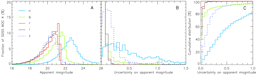
The fourth release of the MOC contains non-photometric nights in the dataset. The SDSS provides data checks that indicate potential problems with the measurements111http://www.sdss.org/dr4/products/catalogs/flags.html, http://www.sdss.org/dr4/products/catalogs/flags_detail.html, http://www.sdss.org/dr7/tutorials/flags/index.html, http://www.astro.washington.edu/users/ivezic/sdssmoc/moving_flags.txt. , and we thus remove observations with flags relevant to moving objects and good photometry: edge, badsky, peaks too close, not checked, binned4, nodeblend, deblend degenerate, bad moving fit, too few good detections, and stationary. These flags note issues such as data where objects were too close to the edge of the frame, the peaks from two objects were too close to be deblended, the object was detected only in a 4x4 binned frame, or the object was not detected as moving. Further details of the flags are provided on the websites in the footnotes. The presence of these flags does not necessary imply problematic data, but because the observations removed due to these flags represent a small percentage of the total objects that fall within the magnitude and photometric error constraints (2%), we prefer to slightly restrict the sample than to contaminate it. Of the 471,569 observations in MOC4 we have a sample of 58,607 observations after applying the selection criteria. We keep observations that are flagged as having interpolation (37% of our sample), including psf flux interp (26% of our sample) which indicates that over 20% of the point spread function flux is interpolated. We also include observations corrected for cosmic rays (6.5%) and those that might have a cosmic ray but are uncorrected (1.5%). Anyone wishing to use the SDSS data or classification results to analyze particular objects rather than large populations is cautioned to note all flags associated with an observation.
2.2 Average albedo of each taxonomic class
There have been recent efforts to determine average albedos per taxonomic class (Ryan and Woodward 2010, Usui et al. 2011, Masiero et al. 2011). These results can be used to more accurately estimate the diameter of a body of a given taxonomic class. In some cases, however, the results disagree by more than the reported uncertainties (e.g., B-types, see Table 1). We calculate mean values, weighted by the number of albedos determined and their accuracy, for each taxonomic class for this work based on averages reported from previously published results (Ryan and Woodward 2010, Usui et al. 2011, Masiero et al. 2011). See Table 1 for a summary of published values and the averages we use in this work. It must also be noted that the average albedo per class does not necessarily represent the actual albedo for any particular object because albedo may vary greatly among each class (e.g., Masiero et al. 2011).
The X class is divided into three classes, E, M, and P, distinguished solely by their albedo (P 0.075, 0.075 M 0.30, E 0.30). We calculate average albedo in each class from the roughly 2,000 objects in our sample that have WISE, AKARI, or IRAS albedos. We find average albedos of 0.45, 0.14, and 0.05 for E, M, and P, respectively. Because the average albedo for a given class is calculated solely using objects with spectral data, and the spectral measurements are biased toward brighter, higher albedo objects, this average could consequently be biased toward higher albedos.
| IRAS | AKARI | WISE | Average | |||||
|---|---|---|---|---|---|---|---|---|
| Class | # | a | a | # | a | # | a | a |
| A | 4 | 0.26 0.12 | 0.18 0.04 | 6 | 0.23 0.06 | 5 | 0.19 0.03 | 0.20 0.03 |
| B | 2 | 0.26 0.13 | 0.08 0.09 | 3 | 0.14 0.03 | 2 | 0.12 0.02 | 0.14 0.04 |
| C | 42 | 0.08 0.02 | 0.06 0.01 | 44 | 0.06 0.03 | 32 | 0.06 0.03 | 0.06 0.01 |
| D | 11 | 0.08 0.03 | 0.07 0.03 | 14 | 0.06 0.03 | 13 | 0.05 0.03 | 0.06 0.01 |
| K | 12 | 0.16 0.07 | 0.12 0.04 | 14 | 0.14 0.04 | 11 | 0.13 0.06 | 0.14 0.02 |
| L | 12 | 0.14 0.04 | 0.11 0.04 | 16 | 0.12 0.04 | 19 | 0.15 0.07 | 0.13 0.01 |
| Q | 1 | 0.51 0.10 | 0.41 0.08 | 1 | 0.28 0.01 | 1 | 0.15 0.03 | 0.27 0.08 |
| S | 50 | 0.26 0.06 | 0.20 0.06 | 104 | 0.23 0.05 | 121 | 0.22 0.07 | 0.23 0.02 |
| V | 1 | 0.37 0.08 | 0.35 0.07 | 1 | 0.34 0.01 | 8 | 0.36 0.10 | 0.35 0.01 |
2.3 Average density of each taxonomic class
To convert from number of objects to
mass, the average density for each class is crucial.
Recently, an order of magnitude improvement of the sample of
asteroid density estimates to 287 allowed the computation of the average density
for each taxonomic class (Carry 2012).
In that work, multiple average densities are reported
depending on the cutoff quality of measurements included.
For the
densities used in this work we chose the average densities using only the
highest quality measurements (despite the smaller sample size). While
these values are certainly an improvement over assuming the same density
for all asteroids, there is still significant uncertainty in the real
densities for any single object, and there is likely a correlation between
density and size particularly due to differences in macroporosity
(see Carry 2012, for details).
Because we use such a large sample, the differences between
any single asteroid and the average should have only a minor
effect on the outcome.
For E, M, and P class objects no average density was reported in
Carry (2012). In
this work we take all objects with densities in each of those classes and
calculate average densities for each class. We find densities of
= 2.8 1.2,
= 3.5 1.0, and
= 2.7 1.6 g/cm3.
The density of M-types is the highest which is consistent with the
current interpretation for their composition.
Some objects in that class are thought to be metallic,
and to contain significant amounts of dense iron
(e.g., Gaffey et al. 1989, Lipschutz et al. 1989, Bell et al. 1989).
However, the M-class is
degenerate in both visible spectrum and geometric albedo because multiple
kinds of asteroids are known to fall in that category each having
different composition and density
(see Rivkin et al. 2000, Shepard et al. 2008, Ockert-Bell et al. 2010, among others).
Not enough data are available to
confidently distinguish the distributions of the different objects falling
in the M-class so we group them together in this work. Additionally, as no
density measurements are available for the D class, we assign an average
density of 1 g/cm3, a density consistent with
comets and transneptunian objects from the outer solar
system (Carry 2012).
3 Observing Biases
Asteroid observations over visible wavelengths are subject to
multiple biases, and the SDSS dataset is no exception. Detection
biases for automatic surveys (relevant to discovery surveys as well
as SDSS) are due to properties of the asteroid (such as size, albedo,
and distance), the physical equipment (such as telescope size and CCD quality),
the scan pattern of the sky,
and the software’s automatic detection algorithm.
For a thorough description
of asteroid observing biases see
Jedicke et al. (2002).
Efforts to correct
the observed asteroid distribution from observing
biases have been undertaken for decades
(Chapman et al. 1971, Kiang 1971, Gradie and Tedesco 1982, Gradie et al. 1989, Bus 1999, Stuart and Binzel 2004). One of the most
significant is a bias toward observing objects with the highest apparent brightness
(objects that are larger, closer, or have a higher surface albedo). This
bias is particularly important for the smallest asteroids, where the
incompleteness of observed versus as-yet undiscovered asteroids is
considerable for any magnitude-limited survey.
The basis of relating the information in the given dataset to the entire
suite of asteroids done here is fundamentally the same as in most previous
work, however, it is executed slightly differently. In previous work
(e.g., Kiang 1971, Chapman et al. 1971, 1975, Gradie and Tedesco 1982, Zellner et al. 1985, Bus 1999, Bus and Binzel 2002b, Mothé-Diniz et al. 2003)
the asteroid belt is broken
up into bins based on orbital elements (typically semi-major axis but some
works include inclination as well) and brightness (earlier works used
the apparent magnitude in V but later works used the absolute magnitude H).
A correction factor is calculated
as the total discovered numbered objects in each bin divided by the total number
of objects in each bin in the given dataset. Each object in the dataset is then multiplied
by the appropriate correction factor.
In this work we determine the fraction of each taxonomic class in each bin from
our dataset and apply those fractions to the total number of discovered objects.
These methods are most accurate if the original dataset is essentially an unbiased
dataset and assume the relative fractions in each bin in the given dataset represent
the actual relative fractions of all asteroids. We describe in this work many steps to
both minimize bias in the dataset and to most accurately compare objects of similar
size. These include using the average albedo per taxonomic class to move from an
H magnitude-limited to diameter -limited sample and correcting for discovery
incompleteness at large H magnitudes. This work accounts for both the sensitivity
difference between the inner and outer parts of the belt and uses a dataset sensitive
enough to probe to very small sizes.
Many of the previous spectroscopic surveys were subject to a target selection bias.
These surveys focused more heavily on objects within asteroid families making the
sample weighted more strongly toward these objects. Previous work
included a correction for these biases (e.g., Bus and Binzel 2002a, Mothé-Diniz et al. 2003). However, because the SDSS is an automated
survey that does not specifically target any type of objects or region of
the belt it does not have the bias of many of the asteroid spectroscopic
surveys that targeted specific regions.
It is also arguable that, even after correcting
for this selection bias, counting family members overweights the
importance of the original parent
body in terms of overall compositional distribution.
Even with an ideal, unbiased dataset, if one counts each asteroid with an
equal weight (for example, by number) the compositional distribution
will be heavily weighted toward the asteroid families even though all the
family members are essentially of the same composition and
originate from the same body. This is fine for studies of number distributions, but
not for the distribution of total material.
A way to mitigate this oversampling of families is to explore the distribution
in terms of volume or mass as explained in the introduction. In this case we are
counting all contributed material of the family; in essence we are putting the
ejected fragments back together again and accounting for the total amount
of material.
Accounting for the bias amongst the smallest asteroids is common to
many datasets. Unique to SDSS compared to previous spectroscopic work
is the bias against observing the largest, brightest asteroids because they
saturated the SDSS detector. Any study of the SDSS sample
would need to correct for the missing large asteroids.
4 Defining the least-biased subset
4.1 Corrections for the largest, brightest asteroids
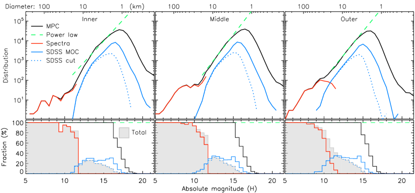
SDSS did not have the capability to measure the largest, brightest asteroids. Conveniently, past spectroscopic surveys are nearly complete at these sizes and fill in that gap (Fig. 1).
We include the taxonomic classes for 1,488 asteroids with an absolute magnitude H 12 determined using spectroscopic measurements in the visible wavelengths (Zellner et al. 1985, Bus and Binzel 2002b, Lazzaro et al. 2004, DeMeo et al. 2009), available on the Planetary Data System (Neese 2010). We keep only the large objects from these surveys where spectroscopic sampling is nearly complete (90%). The smaller objects in the spectroscopic surveys (H 12) were not included in this work because they are more subject to observing biases and selection criteria (Mothé-Diniz et al. 2003). If an object was observed both in the spectroscopic surveys and the SDSS dataset, we use the data and classification from the spectroscopic surveys.
4.2 Corrections for the smallest, dimmest asteroids
Rather than extrapolating into regions in which we have no data that could misrepresent reality, we instead remove the biased portions of the data. We determine the size of the smallest, dark asteroid at a far distance (in this case, the outer belt) at which the SDSS survey is highly efficient. This number is based on the magnitude limits given by Ivezić et al. (2001) and the turnover in objects detected in the survey as a function of size (described in the next paragraph). We then remove any asteroids from the sample that are smaller than that limit. In essence, we create a sample restricted by a physical rather than an observable quantity: a diameter-limited instead of an apparent magnitude-limited sample.
Taking the SDSS sample, we determine the
largest absolute magnitude (H) at which the survey is sensitive for each
zone.
We present in Fig. 1 the number of objects
and fraction of the sample covered by the spectroscopic surveys as well as
the fraction the SDSS covers relative to all discovered and undiscovered
asteroids for a large range of absolute magnitudes.
The peak of the black solid line in Fig. 1
represents the limit of
discovery efficiency for zones of the main belt. The cutoff magnitudes are
roughly 17.2, 16.5, 15.5, 14.5, and 12.5 for the inner (IMB), middle
(MMB), and outer Main Belt (OMB), Cybeles and Hildas, and Trojans,
respectively.
We use these absolute magnitude limits to define the asteroid size range for
which a distribution study can be reasonably confident. The smallest size
sampled among all asteroid types is limited by the darkest, farthest
objects (P-type, see Table 2).
For our sample we use the outer main belt
to determine our size cutoff. It would be preferable to use the Hilda or
Trojan regions, because then we explore the same size range from the main
belt out to the Trojans. However, this would drastically limit our
sample size. It is thus important to recognize that our results do not
contain Hildas and Trojans down to as small sizes as in the main belt.
In our sample, the number of Hildas and Trojans is severely biased toward
larger sizes, however, because these populations contain asteroids
all with similarly low albedos
(Grav et al. 2011, 2012a, 2012b)
there is no significant bias on the relative
number of bodies of each taxonomic class. For this reason we include
the Hildas and Trojans in the present work.
The smallest P-type asteroids the SDSS surveyed in the OMB have H=15.5
which represents a diameter of 5 km. While we sample, for
example, S-types in the outer belt and C-types in the inner belt with
diameters of 2 km and S- and V-types in the inner belt to 1 km or less,
including these smaller objects in
our sample would bias the results in terms of number toward
these smaller objects that are not sampled in the outer belt.
Instead we
include in our sample only objects that are 5 kilometers or larger.
This size is equivalent to a different H magnitude for each class.
The ratio of each taxonomic class’ albedo (, where is the
taxonomic class) with the P-type albedo () can be used to determine the
magnitude difference between same-size objects of different taxonomic
classes using the equation
| (1) |
We cut the sample of each taxonomic class according to these H magnitude
limits, which are listed in Table 2.
The average albedo for each class
was determined by taking the average of the albedo determined for each
class from IRAS, AKARI, and WISE
(Ryan and Woodward 2010, Usui et al. 2011, Masiero et al. 2011, see Sec. 2.2).
Using a different H magnitude for each taxonomic class is
critical. If we cut our sample at H=15.5 for all objects we would be
comparing, for example, 5 km P-types to 2 km S-types, which are
much more numerous owing to the steep size-frequency distribution of
the asteroid population.
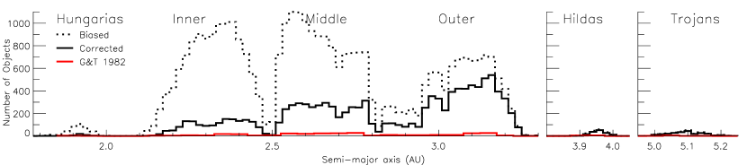
The size of the SDSS sample before and after the bias-correction
selection is shown in Fig. 3, together with the number of
objects presented in the preceding work by
Gradie and Tedesco (1982). It is clear that a vast
number of objects are removed from the inner and middle sections of the
belt because they are below the critical size limit. To give an
estimate on the importance of this size correction, there are
5,000 5 km asteroids in the middle belt, however there are
about 40,000 2 km ones known, nearly a factor of 10 greater.
| Class | H | Density | Albedo | ||
|---|---|---|---|---|---|
| A | 13.99 | 3.73 | 1.40 | 0.20 | 0.03 |
| B | 14.38 | 2.38 | 0.45 | 0.14 | 0.04 |
| C | 15.30 | 1.33 | 0.58 | 0.06 | 0.01 |
| D | 15.30 | 1.00 | 1.00 | 0.06 | 0.01 |
| K | 14.38 | 3.54 | 0.21 | 0.14 | 0.02 |
| L | 14.46 | 3.22 | 0.97 | 0.13 | 0.01 |
| S | 13.84 | 2.72 | 0.54 | 0.23 | 0.02 |
| V | 13.39 | 1.93 | 1.07 | 0.35 | 0.01 |
| E | 13.12 | 2.67 | 1.20 | 0.45 | 0.21 |
| M | 14.49 | 3.49 | 1.00 | 0.13 | 0.05 |
| P | 15.50 | 2.84 | 1.60 | 0.05 | 0.01 |
5 Taxonomic classification
The SDSS asteroid data has been grouped and classified according to their colors by many authors. Ivezić et al. (2002) classified the C, S, and V groups using the z’-i’ color and the first principal component of the r’-i’ vs r’-g’ colors. Nesvorný et al. (2005) used the first two principal components of u’, g’, r’, i’, z’ colors and distinguished between the C, X, and S-complexes. Carvano et al. (2010) converted colors to reflectance values and created a probability density map of previously classified asteroids and synthetic spectra to classify the SDSS dataset.
In this work we seek to maximize the taxonomic detail contained in the dataset and strive to keep the class definitions as consistent as possible with previous spectral taxonomies that were based on higher spectral resolution and larger wavelength coverage data sets, specifically Bus (Bus and Binzel 2002a) and Bus-DeMeo (DeMeo et al. 2009) taxonomies.
5.1 Motivation for manually defined class boundaries
The best way to mine the most information out of such a large
dataset could be to perform an analysis of the variation and
clustering. Methods such as Principal Component Analysis or Hierarchical
Clustering could separate and highlight groups within the data. The advantage to
automated methods is they are unbiased by human intervention and can
efficiently characterize large datasets, which are the motivations for
many unsupervised classifications.
However, because most of our understanding of asteroid mineralogy comes
from relating asteroid spectral taxonomic classes to meteorite classes
and comparing absorption bands, we find it more relevant to connect this
low-resolution data to already defined and well-studied asteroid
taxonomic classes (that were based on Principal Component
Analysis). This facilitates putting the SDSS results in context
with the findings from other observations that have accumulated over
decades. To classify the data we started with the class centers and
standard deviations (based on data used to create the Bus-DeMeo taxonomy
converted to SDSS colors) to
calculate the distance of each object to the class center.
Considering the above, while we still use the class centers and
calculated deviations as a guide, we choose to fix boundaries for each
class and manually tweak them (as described below) according to the data
to best capture the essence of each class. A negative consequence of
fixed boundaries is that near the boundary objects exist on either side
that may have very similar characteristics though are classified
differently (as opposed to methods which assign a probability for each
object to be in a certain class). Additionally, a human bias is
added. The advantage, however, is we are forced to carefully evaluate
the motivation for the definition of each class to group objects
according to the most diagnostic spectral parameters (particularly
considering the much wider spread of the SDSS dataset), consistency with
previous classifications, and potential compositional
interpretation. Additionally, fixing the boundary allows us to more easily use the
classifications as a tool. We can use these
classifications to determine the fraction of objects in each class and
the mass of each taxonomic type across the solar system.
5.2 Defining the class boundaries
We transform the apparent magnitudes from SDSS to reflectance values to directly compare with taxonomic systems based on reflectance data. We then subtract solar colors in each filter and calculate reflectance values using the following equation:
| (2) |
where () and () are the magnitudes of the object and sun in a certain filter , respectively, at the central wavelength of the filter. The equation is normalized to unity at the central wavelength of filter g using () and (): the magnitudes of the object and sun, respectively. Solar colors used in this work are r’-g’= -0.45 0.02, i’-g’= -0.55 0.03, and z’-g’= -0.61 0.04 from Holmberg et al. (2006). Note that because we use solar colors in the Sloan filters we do not convert from the g’, r’, i,’ z’ filters (central wavelengths: g’=0.4686, r’=0.6166, i’=0.7480, z’=0.8932 m) to standard g, r, i, z filters. As mentioned in Section 2.1, we do not use the u’ filter because of the very large errors for this datapoint.
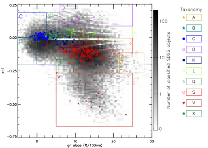
The classification of the dataset is based on two dimensions: spectral slope over the g’, r’, and i’ reflectance values (hereafter gri-slope), representing the slope of the continuum, and z’-i’ color, representing band depth of a potential 1 m band. We restrict the evaluation of the spectral slope to g’, r’, and i’ filters only, excluding the z’ filter because it may be affected by the potential 1 m band. These two parameters (slope and band depth) are the most characteristic spectral distinguishers in all major taxonomies beginning with Chapman et al. (1975) because they account for the largest amount of meaningful and readily interpretable variance in the system.
We choose not to use defined by Ivezić et al. (2002) or the first Principal Component (PC1) defined by Nesvorný et al. (2005) used in other works. is the first principal component of the r’-i’ versus g’-r’ colors and PC1 is the first principal component of the measured fluxes of all five filters. To most effectively use Principal Component Analysis, the dimension with the greatest variance, slope in this case, should be removed before running PCA to increase sensitivity to more subtle variation (see discussion in Bus 1999). We also disfavor the inclusion of the u’ filter (used for PC1) as it adds significant noise to the data (Fig 2). We find our slope parameter is reasonably well-correlated with but not well-correlated with PC1, as expected from the use of u’ photometry in PC1.
We base the classification on the 371 spectra used to create the Bus-DeMeo taxonomy (DeMeo et al. 2009), whose classes are very similar those of the Bus taxonomy (Bus and Binzel 2002a), with a few classes removed. The variation among the reflectance spectra of the 371 asteroids used to define the Bus-DeMeo classes helped guide the boundary conditions of the present SDSS taxonomy. We convert all the spectra into SDSS reflectance values by convolving them with the SDSS filter transmission curves222 http://www.sdss.org/dr7/instruments/imager/, thus providing the average SDSS colors and standard deviation per class (see Fig. 4)
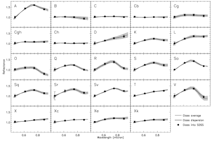
Because the SDSS data have a spectral resolution significantly lower than the Bus-DeMeo data set (see Fig. 4) and subtle spectral details are lost, we combine certain classes into their broader complex. The C-complex encompasses the region including C-, Cb-, Cg-, Cgh-, and Ch-types. The S-complex encompasses the S-, Sa-, Sq-, Sr-, and Sv-types. The X-complex includes X-, Xc-, Xe-, Xk-, and T-types. The classes that are maintained individually are A, B, D, L, K, Q, and V. While we distinguish all these classes based on the SDSS colors here, we slightly modify our use of some of these classes for this work (see Section 6.1). We do not classify the rare R- or O-type in this work, because there is significant overlap between O-types or R-types and other classes in the visible wavelength range, and they are particularly rare classes. The R class would overlap the V class essentially spanning the shallower z’-i’ “band depth” region. We tested separating the R class, but the majority of the objects classified as R were located in the Vesta family.
While the Bus-DeMeo class averages are very useful as a guide, the system was based on a sample size three orders of magnitude smaller than present SDSS sample. The SDSS dataset therefore shows a much more continuous range of reflectance characteristics. To compare the two datasets, we plot the distribution of SDSS objects in z’-i’ color and gri-slope, with the 371 objects from the Bus-DeMeo taxonomy (Fig. 5). Furthermore, the figure shows the boundaries for each class defined in this work. We drew boundaries that best separated each class based on the position of the class centers and standard deviations based on the 371 spectra dataset. We visually inspected each boundary by plotting the spectral data on each side of the boundary and comparing them with the designated class to tweak the position of the line and best separate each class.
We strove to preserve the uniqueness of the more exotic classes, restricting A- and D-types to the outliers with the largest slopes, and Q- and V-types with the deepest bands. The B-type was defined to have both a large, negative gri-slope and a negative z’-i’ value. A list of all the boundaries is provided in Table 3. Classification is performed in decision tree form, where the gri-slope and z’-i’ value of the asteroid is compared with each region in the following order: C, B, S, L, X, D, K, Q, V, A. If the object falls in more than one class, it is designated to the last class in which it resides. As can be seen in Fig. 5, there are a handful of objects that reside outside the defined classes. We give these objects the designation “U”, historically used to mark unusual objects in a sample that do not fall near any class. We do not include these objects in our study. Most of these extreme behaviors are likely due to problems with the data even though no flags were assigned (see details in Section 2.1). Follow-up observations could determine whether the objects really are unique.
| Class | Slope (%/100 nm) | z’-i’ | ||
|---|---|---|---|---|
| (min) | (max) | (min) | (max) | |
| A | 21.5 | 28.0 | -0.265 | -0.115 |
| B | -5.0 | 0.0 | -0.200 | 0.000 |
| C | -5.0 | 6.0 | -0.200 | 0.185 |
| D | 6.0 | 25.0 | 0.085 | 0.335 |
| K | 6.0 | 11.0 | -0.075 | -0.005 |
| L | 9.0 | 25.0 | -0.005 | 0.085 |
| Q | 5.0 | 9.5 | -0.265 | -0.165 |
| S | 6.0 | 25.0 | -0.265 | -0.005 |
| V | 5.0 | 25.0 | -0.665 | -0.265 |
| X | 2.5 | 9.0 | -0.005 | 0.185 |
5.3 Determining a single classification for multiple observations
Of the many observations in the SDSS MOC that remained after we applied cuts on the photometric precision (58,607, see Section 2.1), many were actually the same object observed more than once. The number of unique objects in our sample is 34,503. For some of these objects, not all observations fell into the same class. Because we seek to categorize each object with a unique class, we use the following criteria to choose a single class for any object that has multiple observations that fall under multiple classifications (5,401 asteroids, i.e., 15.7% of the sample):
-
1.
The class with the majority number of classifications is assigned (2,619 asteroids, i.e., 7.6% of the sample)
-
2.
If two classes have equal frequency and one of them is C, S, or X we assign the object to C, S, or X, continuing the philosophy of remaining conservative when assigning a more rare class (1867 asteroids, i.e., 5.4% of the sample)
-
3.
If the two majority classes are C/S, X/C, S/X (or three competing classes of C/S/X) we assign it to the U class and disregard those objects in the distribution work (919 asteroids, i.e., 2.6% of the sample). We prefer to keep the sample smaller, rather than contaminate it with objects that we have randomly chosen a classification among C, S, or X and thus possibly bias the sample.
-
4.
For objects that are assigned multiple classes but none is either the majority or C, S, or X is assigned to the U class.
Among the largest asteroids, particularly those between H magnitudes of 9 and 12, several asteroids observed by the SDSS had taxonomic classes from previous spectroscopic measurements. The classification based on SDSS and previous work were generally consistent, but in cases that differed, we assigned the asteroid to the class determined by spectroscopic measurements.
5.4 Caution on taxonomic interpretation
One must be careful when interpreting the classifications presented here. First, the resolution of the SDSS data are significantly lower than the spectra to which they are compared. Second, the fact that we find multiple classifications for multiply observed objects suggests there is a larger uncertainty in the data than expected. Third, for many classes (particularly L, S, Q, A), the visible data can only suggest the presence of a 1 m band, but do not actually predict the depth or shape of that band (for more detail see DeMeo et al. 2009, DeMeo 2010). This is important because, for example, a spectrum might look closer to a K- or an L-type in the visible range, but near-infrared data could place them more confidently in the S-class (or vice versa).
Each class is meant to be representative of a certain spectral characteristic, but with limited wavelength coverage and limited resolution, there is some degeneracy. For example, the Q-class defined here represents objects with a low slope and moderate 1 m band depth. We do not suppose that all objects classified as a Q-type are young, fresh surfaces as is typically associated with the Q class. Careful follow-up observations are important to make such a claim.
Defining boundaries for C, X, and D-types is not easy because they are distinguished only by slope and there is a continuous gradient of slope characteristics. This problem is not unique to the SDSS dataset. The boundary between each type is somewhat arbitrary. The difference between a C-type of slope zero and a D-type with a high slope is meaningful, however we do not yet know how to interpret the significance of these spectral differences. It is likely that there is some contamination between C- and X-types with our classification scheme, though it is unlikely that much contamination exists for example between C- and D-types that are more easily distinguished.
5.5 Verification of our classifications
With a unique class assigned to each object in our dataset we can now evaluate the robustness of our classifications. First, we compare the classification of each asteroid with the results of Carvano et al. (2010) available on the Planetary Data System (Hasselmann et al. 2011). Because their classification is based on the same dataset, it is not an entirely independent check. However, their classification method is different so consistency between the two supports both methods. Fig. 6 graphically compares the two classifications. We list the classification differences that are generally compatible but represent the different choices each method made. We find the two classifications quite consistent. Of the major classification differences between the two methods we suspect some are due to boundary condition differences and others are due to Carvano’s inclusion of the u’ filter, which we exclude in our work (see Sec. 2.1).

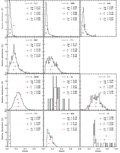
Second, we retrieved the albedo of the asteroids as determined
from IRAS, AKARI, and WISE data
(Tedesco et al. 2002, Ryan and Woodward 2010, Usui et al. 2011, Masiero et al. 2011, 2012, Grav et al. 2011, 2012a, 2012b).
We found 17,575 asteroids (out of 34,503, i.e., 51%) with albedo
determinations. We present in Fig. 7 the distribution of
albedo for each class, and the average values in Table 4.
The agreement between the average albedo per Bus-DeMeo class from previous
work (see Table 1) and of the
asteroids classified from SDSS colors gives confidence in our capability
to assign a relevant class to these asteroids.
One of the greatest differences is the albedo
of the B class.
| Class | Nobjects | Average | Mode | ||
|---|---|---|---|---|---|
| A | 32 | 0.274 | 0.093 | 0.258 | 0.055 |
| B | 833 | 0.071 | 0.033 | 0.061 | 0.021 |
| C | 4881 | 0.083 | 0.076 | 0.054 | 0.023 |
| D | 546 | 0.098 | 0.061 | 0.065 | 0.026 |
| K | 892 | 0.178 | 0.099 | 0.146 | 0.075 |
| L | 711 | 0.183 | 0.089 | 0.157 | 0.088 |
| S | 6565 | 0.258 | 0.087 | 0.247 | 0.084 |
| V | 711 | 0.352 | 0.107 | 0.345 | 0.104 |
| E | 47 | 0.536 | 0.247 | 0.322 | 0.016 |
| M | 825 | 0.143 | 0.051 | 0.115 | 0.051 |
| P | 771 | 0.053 | 0.012 | 0.053 | 0.012 |
We have separated the spectra of objects with negative slopes into the B class using SDSS colors as has traditionally been done in taxonomic systems. This separation can be a useful indicator of spectral differences between B and C classes. The average albedo for B-types classified from spectroscopic samples is significantly higher than for C-types (see Table 1) suggesting a compositional difference. However, the average albedo of B-types in our SDSS sample is similar to that for C-types so we caution that the B-types classified from spectroscopic surveys may not be fully representative of the B-types in our sample.
6 Building the compositional distribution
6.1 Additional taxonomic modifications
Keeping in mind the cautions mentioned in Section 5.4,
for the taxonomic distribution work presented here
we apply slight modifications to the
classes. First, we note a significant over abundance of S-types in the Eos
family. This is due to the similarity of S- and K-type spectra
using only a few color points and the visible-only wavelength range. We
thus reclassify all S-type objects to K-type within the Eos family
(defined by the family’s current orbital elements
a [2.95, 3.1],
i [8∘, 12∘], and
e [0.01, 0.13]).
Reviewing this change shows that the background of S-types
is now evenly distributed, no longer showing a concentration within the
Eos family. Additionally, for this study we group Q-types with the S-types
because they are compositionally similar (Binzel et al. 2010, Nakamura et al. 2011).
In the previous section we discussed the albedo differences
between B-types in our sample and B-types from other work.
While future work may want to focus specifically on objects
with negative slopes, in this we choose to merge B-types
with C-types classified by the SDSS dataset.
Our SDSS observations classify some Hildas and Trojans as K- and L-types.
Careful examination reveals that for the K- and L-
type objects that are near the border the X and D classes, the spectra could also be
consistent with X and D. These Hilda and Trojan K- and L-types that have multiple observations are
also classified X and D. For example, the Centaur (8405)
Asbolus has a very red visible spectral slope
(Barucci et al. 1999), categorizing it as a D-type.
Eight SDSS observations place this object in the L class and four
in the D class. This difficulty is partially due to the degeneracy of the
visible wavelength data. The Bus Ld class
that is intermediate between the
L and D classes does not remain an intact definable class when
near-infrared data are available
(DeMeo et al. 2009). There are four SDSS L-type Hildas and
Trojans with albedos all of which are below 0.08 further suggesting that
these objects are not characterized by what the K and L classes are
compositionally meant to represent.
We therefore choose the
more conservative option to reclassify
the Hilda and Trojan K- and L-types. The K-types that have slopes
more consistent with the X class are relabeled as X, while the L-types
have slopes more consistent with D-type and are relabeled as D.
Among the Hungarias, a population of small (H 13) C-types is
seen. Upon
closer inspection, all (8) of the small C-types with WISE data have
extremely high albedos (0.4–0.9), suggesting they are actually
E-types (the high albedo group of X-types). This is unsurprising, as the
Hungaria region is known to contain
a large population of high albedo E-type asteroids. We thus correct our
Hungaria sample by assuming all small C-types are incorrectly classified,
and remove those with H magnitudes greater than the E-type cutoff from our
sample. We expect some overlap between C-types and X-types (E, M, P)
in other regions of the belt as well (as addressed in Sec. 5.4)
although the classification of X v. C should be more balanced.
While we make these modifications for the objects in the SDSS sample
we do not make changes to the large objects classified spectroscopically from
previous work.
6.2 Discovery completeness
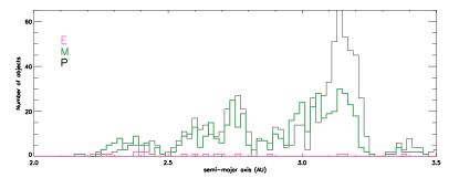
While we select the subset of SDSS data where the survey is efficient, the dataset not complete. The information from the SDSS dataset must be applied to all existing asteroids in the same size range. The Minor Planet Center (MPC) catalogues all asteroid discoveries. Here we asses discovery completeness.
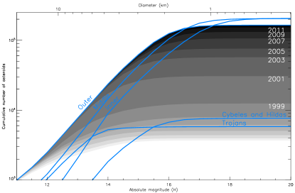
In Fig. 8, we plot the cumulative number of
discoveries in the outer belt for every two years of the past 10 years (to
2013-01-01).
We derive a limiting magnitude for the completeness of the
MPC database of H = 16, 15 and 14.5 (diameter of about 2, 3, and 4 km) for
the inner, middle, and outer belt, respectively.
We determine the completeness of small asteroids in each section of
the main belt by extrapolating the size of the population using a power
law fit to each region of the main belt
(shown in Fig. 1).
The difference between the currently observed populations and the extrapolated
populations derived from these power laws provide the expected number of
asteroids to be discovered at each size range.
The power law indices we find for the
IMB, MMB, and OMB (determined over the H magnitude range
14–16,
13–15, and
12–14.5) are -2.15, -2.57, and -2.42, respectively. These power law indices
agree with other fits to the observations
(Gladman et al. 2009) as well as with the
theoretical index calculated assuming a collision-dominated
environment (Dohnanyi 1969).
For almost all H magnitudes
in our sample we are nearly discovery complete. For the smallest size
we use a power law function to determine completeness.
In the H=15-16 magnitude range, we are
100%, 85%, and 60% complete in the IMB, MMB, and OMB respectively.
When applying the
taxonomic fractions to the MPC sample of known asteroids we add
a correction factor to account the 15% and 40% of objects that
have not been discovered in the middle and outer belt in the H=15-16 range.
For Cybeles, Hildas, and Trojans we do
not extrapolate to determine sample completeness because there is far too much
uncertainty in the size distribution of those populations due to fewer
discoveries. We have not corrected these populations.
The completeness of our dataset can be evaluated on
Fig. 1.
There are undoubtedly still many objects yet to be discovered, especially
at sizes smaller than we cover in this work. For reference, we explore the
total mass these undiscovered objects are expected to represent. The
largest objects represent the overwhelming majority of the mass in the
main belt. In fact, the asteroids from the spectral surveys (particularly H10)
represent 97% of the mass
(assuming a mass of 30 1020 kg for the entire main belt,
Kuchynka and Folkner 2013).
We calculate the undiscovered mass (assuming a general
density of 2.0 g/cm3 and an albedo of 0.18, 0.14, and 0.09 for the
inner, mid, and outer main belt, based on WISE
measurements, see Mainzer et al. 2011) up
to H magnitude of 22 to be
5.7 1012,
4.8 1013, and
1.6 1014 kg for the
IMB, MMB, and OMB, that each contain a total mass (with the same generic albedo
and density assumptions) of
6.2 1020,
1.3 1021, and
7.1 1020 kg,
with a total of 26 1020 kg.
Therefore, although hundreds of thousands of asteroids
will still be discovered and they will provide valuable information about asteroids
at small size scales, their expected contribution in terms of mass is minuscule
(below the part per million level).
6.3 Applying the SDSS distribution to all asteroids
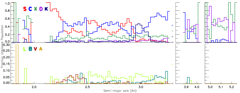
After applying data quality cutoffs, H-magnitude cutoffs, and taxonomic classifications, we can now calculate the number of SDSS objects in each class according to size and distance. We use H magnitude bins of 1 magnitude ranging from 3 to 16 (though each class has its appropriate H magnitude cutoff listed in Table 2). The semi-major axis bins applied are 0.02 AU wide ranging from 1.78 to 5.40 AU. Only asteroids among Hungarias, the main belt, Cybeles, Hildas and Trojans are included in this study covering the distances 1.78-2.05, 2.05-3.27, 3.27-3.7, 3.7-4.2, and 5.05-5.40 AU, respectively. Near-earth objects, comets, Centaurs, Transneptunian objects and any other objects outside the mentioned zones were excluded. We calculate the number of objects in each bin and the fraction of each class in each bin (Fi, where i is the taxonomic class). For example, for objects with H magnitudes between 13 and 14 and semi-major axes between 2.30 and 2.32 AU, we might find 60% of the objects are S-type (Fs = 0.6), 20% are C-type (Fc = 0.2), 20% are X-type (Fx = 0.2). Figs 9 and 10 show the bias-corrected and biased fraction of objects. The biased view of the asteroid belt shows a dominance of S-types (by number) out to nearly 3 AU because of the inclusion of the abundant smaller, higher albedo bodies (whose small, dark counterparts, the C-types, were not observed). The bias-corrected version demonstrates that instead, the S-types and C-types alternate dominating by number throughout the belt. Asteroid families play an important role in these figures since they contribute large numbers of taxonomically similar objects.
Albedo data enable the separation of X-types into three sub groups: E, M, P (Tholen 1984). Since albedo data are not available for every single spectral X-type, we calculate the fraction of E, M, and P for each region: Hungaria, Inner, Middle, Outer, Cybele, Hilda, Trojan. This fraction is calculated based on 2000 X-type objects in our sample with albedo measurements (from a total of 2500 X-types) from IRAS, AKARI, and WISE (Ryan and Woodward 2010, Usui et al. 2011, Masiero et al. 2011). See Fig. 11 for the bias-corrected distribution of the E, M, and P types across the main belt that was used to extrapolate the X-type EMP fraction for our entire dataset. Among Hungarias the sample is entirely E-type as expected. There are an insignificant number of E-types among the other regions (though we note a bias against observing high visible albedo objects in mid-infrared wavelength ranges). The fraction of all bias-corrected X-types that are M in each region are: 0.00, 0.58, 0.44, 0.35, 0.28, 0.08, and 0.17, respectively. The fraction for P-types is thus one minus the M-type fraction, except for the Hungaria region where it is also zero. Among Trojans we find that 0.17 (1 out of 6) X-types have an M-type albedo, however because of large uncertainty due to a small sample we assume the same fraction for Trojans as Hildas (0.08).
We now know the relative abundance of each taxonomic type at each size range and distance
determined from the SDSS dataset with and adjustment for the division of
E, M, and P types from the X class.
However, at many size ranges the SDSS only observed 30%
of the total asteroids that exist at that size and distance. As long as we only use a
size range in which asteroid discovery is essentially complete or make a correction for
discovery incompleteness, we can apply these fractions to
the entire set of known asteroids at these sizes from the Minor Planet Center to determine
the distribution of taxonomic type across the main belt according to number, surface area, volume,
and mass.
When calculating the number of objects, surface area, volume, or mass at each size range and distance we use two different methods. For the largest asteroids with H 10 where our SDSS sample is complete, we calculate the surface area, volume, or mass for each asteroid using that body’s H magnitude, albedo (or average albedo for its taxonomic class when not available), and average density (Carry 2012) for that taxonomic class.
For objects with 10 H 13, where our sampling is not complete, we use the following method. The surface area, volume, or mass is calculated for an object using the H magnitude, average albedo and average density for that class. That value is multiplied by the number of objects of that class in that bin (Ni) which is the the total number of known asteroids in that (size and distance) bin, Nbin, and by the fraction (Fi) of objects of that class from SDSS: Ni=Nbin Fi.
For objects with H13 we have the added complication that we cannot directly apply our fraction to the total number of known objects because our fraction of each type at each size from SDSS is calculated with certain (higher albedo) classes removed. We thus must also calculate the fraction of objects in the SDSS database that were kept, Fkept, (i.e., those that were not removed because they are smaller than 5 kilometers) for H magnitude bins H=13, 14, and 15. For all other size bins Fkept is equal to 1. The number of objects of a certain class (Ni) can be determined by the total number of discovered objects in that bin (Nbin) multiplied by the fraction of objects in that class (Fi) and by the fraction of objects in that bin that are kept (Fkept), thus Ni=Nbin Fi Fkept.
Previously in this section, we calculated the bias-corrected fraction of E, M, and P types in each zone, although, as above, we cannot apply this true (bias-corrected) correction factor to the observed (biased) MPC dataset. For the H bins 14 and 15 where some M-types were removed due to size we calculate the fraction of (M+P)-types kept in each region. The fraction for H=14 is 0.60, 0.67, 0.64, 0.79, for the IMB, MMB, OMB, and Cybeles and 0.22, 0.39, 0.41, 0.70 for H=15. There are no small objects in our sample to be removed in the Hilda and Trojan regions so the fraction kept is unity.
Finally, if we simply assume an average H magnitude for each bin (say 12.5 for the H=12 bin) we could potentially over- or underestimate the surface area, volume, or mass, depending on the H magnitude distribution of objects in that bin. We thus calculate the number of objects in each 0.1 H magnitude sub-bin and apply the same class fractions to each for accuracy.
7 The compositional makeup of the main belt
7.1 Motivation for number, surface area, volume, and mass
Previous work calculated compositional distribution based on the number of
objects at each distance
(e.g. Chapman et al. 1975, Gradie and Tedesco 1982, Gradie et al. 1989, Mothé-Diniz et al. 2003).
This was not unreasonable because those datasets
included only the largest objects, often greater than 50 km in diameter.
If we restrict our study to the number of asteroids, our views
would be strongly influenced by the small asteroids.
There are indeed more asteroids of small size than large ones. This is the
result of eons of collisions, grinding the asteroids down from
larger to smaller.
The size-frequency distribution of asteroids
(Fig. 1) can be approximated by a power-law, and
for any diameter below 20 km, there are about 10 times more asteroids
with half the diameter.
The amount of material (i.e., the volume) of the two size ranges is
however similar: if there are asteroids of a given diameter ,
there are about 10 asteroids with a diameter of , each with a
volume 8 times smaller, evening out the apparently dominating importance
of the smaller sizes.
Ceres alone contains about a third of the mass in the entire main belt using
a mass of 30 1020 kg for the main
belt (Kuchynka and Folkner 2013), and 9 1020 kg for Ceres
(from a selection of 28 estimates, see Carry 2012)),
and yet it is negligible (1 out of 600,000) when
accounted for in a distribution by number.
Therefore, the relative importance of Ceres in the main belt can change by
orders of magnitude depending on how we look at the distribution.
The study of the compositional distribution by
number is perfectly valid and is useful for size-frequency distribution studies
and collisional evolution. For studies of the distribution of the amount
of material, it puts too much emphasis on the
small objects compared to the largest.
A simple way to balance the situation is to consider each object weighted
by its diameter.
This opens new views on asteroids: we can study how much surface area
of a given composition is accessible for sampling or mining purposes
(Section 7.2), or how much material accreted
in the early solar system has survived in the Belt
(Sections 7.3 and 7.4 for the distributions
by volume and mass).
7.2 Asteroid distribution by surface area
To estimate the surface area of each asteroid, we need first to estimate its diameter . For that we use the following equation from Pravec and Harris (2007, and references therein):
| (3) |
where is the absolute magnitude (determined by the
SDSS survey) and is the albedo.
For the largest asteroids (H 10) we use the object’s calculated albedo
from WISE, AKARI, or IRAS. For small asteroids, and large ones for
which no albedo is available, we use the average albedo for that object’s
taxonomic class, see 2.2.
The equation above provides a crude estimation of the diameter only.
Evaluation for a particular target should be considered with caution,
the absolute magnitude and albedo being possibly subject to large
uncertainties and biases (e.g., Romanishin and Tegler 2005, Mueller et al. 2011, Pravec et al. 2012).
We can nevertheless make good use of this formula for statistical
purposes: the precision on the diameters is indeed rough but seemingly
unbiased (Carry 2012).
With a diameter determined for each asteroid, we estimated their
individual surface area
by computing the area of a sphere of the same diameter:
= .
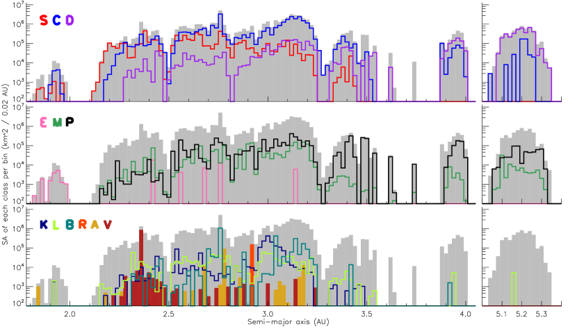
The surface area distribution is presented in
Fig. 12.
The total surface area per bin ranges from 103 km2 in the
Hungarias to 106 in the main belt.
Viewing the distribution with respect to surface area we can
immediately notice the relative importance of larger bodies. Ceres
and Pallas are represented by the blue peak near 2.75 AU and
Vesta by the red peak near 2.35 AU. Additionally the E-types in pink,
distributed throughout the main belt, are each only one or two asteroids.
7.3 Asteroid distribution by volume
While the real value we seek is mass, because the density contributes significant uncertainty to the mass calculation we also present the distribution according to volume of material which gives similar results but is not affected by density uncertainties.
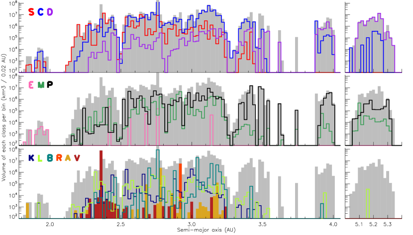
To evaluate the amount of material in the main belt, for each taxonomic class, we estimate the volume of all the asteroids by computing the volume of a sphere of the same diameter: . We use the same method to calculate the total volume distribution by applying SDSS taxonomic fractions to the MPC dataset as described in Section 6.3. By looking at the compositional distribution in terms of volume instead of numbers, most of the issues described in Section 7.1 are addressed. Indeed, if there are about 2500 asteroids with a diameter of 10 km in the main belt, their cumulated volume is 300 times smaller than that of Ceres, re-establishing the proportions. The conversion from numbers to volume also corrects our sample for an overrepresentation of the contribution by collisional families (when viewed by number). Indeed, a swarm of fragments is released during every cataclysmic disruptive event, “artificially” increasing the relative proportion of a given taxonomic class locally (e.g., the Vestoids in the inner belt, see Fig. 10). Here, we are accounting for all the material of the family as if put back together again.
We present the distribution of taxonomic class by volume in Fig. 13. The distribution is the same as for surface area, but with the y-axis stretched because volume is proportional to diameter cubed while surface area is proportional to diameter squared. Asteroid distributions by volume were first presented by Consolmagno et al. (2012).
7.4 Asteroid distribution by mass
Ultimately, the mass is the physical parameter we seek that provides insights on the distribution of material in the solar system. To precisely measure the mass of each asteroid we would need a fleet of missions to fly by each asteroid. Barring that as an option in the foreseeable future, to estimate the mass of each asteroid we need an approximate density together with the estimated volume determined above. The density is the least well-constrained value used in this work because these measurements are extremely difficult to obtain (see discussion in Britt et al. 2002, 2006, Carry 2012). Nevertheless, the study of meteorites tells us that the available range for asteroid density is narrower than it may seem. Indeed, no meteorite denser than 7.7 g/cm3 has ever been found, and most of the meteorites cluster in a tight range, from 2 to 5 g/cm3 (see Consolmagno and Britt 1998, Consolmagno et al. 2008, Britt and Consolmagno 2003, Macke et al. 2010, 2011, and references therein), with the exception of iron meteorites above 7 g/cm3 (see the summary table in Carry 2012). This range may be wider, especially at the lower end, for asteroids due to the possible presence of voids in their interiors, such as the low density of 1.3 g/cm3 found for asteroid (253) Mathilde (Veverka et al. 1997). However, even if we assign an incorrect density to an asteroid, the impact on its mass will remain contained within a factor of 4 at the very worst. The impact may even be smaller as the typical densities of the most common asteroid classes (i.e., C and S) are known with better accuracy (Carry 2012).
The uncertainty on the density will therefore affect the distribution in a much lesser extent than equal weighting of bodies according to number. Of course, any uncertainty on any of the parameters will sum up in the total uncertainty. However, we are confident that the trends we discuss below are real: both the discovery completeness, diameter estimates, and average albedo and density per taxonomic class have become more and more numerous and reliable over the last decade.
To calculate the distribution by mass we apply the average density of each class (Table 2, 2.3) and multiply that by the volume determined in the previous Section. For Ceres, Vesta, Pallas, and Hygiea, the four most massive asteroids we include their measured masses (9.44, 2.59, 2.04, and 0.86 1020 kg, from Carry 2012, Russell et al. 2012) each accounting for about 31%, 9%, 7% and 3% of the mass of the main belt, respectively (using a total mass of the belt of 30 1020 kg, Kuchynka and Folkner 2013)
The distribution of mass is presented in Fig.14 The fractional distribution of each class throughout the belt is given in Fig. 15. Again, we find the general trends to be similar to volume and surface area. The difference in the case of mass is that the relative abundance of the taxonomic types have changed. Because S-types are generally denser than C-types by a factor of roughly 2 we see S-type material is more abundant relative to C than in our previous plots. Because in many cases the relative abundance of different taxonomic types already vary by an order of magnitude or more, we do not see drastic relative abundance changes. For example, C-types contribute more mass to the outer belt than S-types even though their relative abundance by mass is closer than by volume.
7.5 Search for S-types among Hildas and Trojans
We note a sharp cliff at the edge of the outer belt delineating the limit of S-type asteroids. Mothé-Diniz et al. (2003) were the first to show the presence of S-types out to 3 AU in their dataset of asteroids 15 km and greater. We find that almost no S-types exist among Cybeles, and they are entirely absent beyond 3.5 AU.
Despite the bias toward discovering S-types (they reflect 5 times more light than C-, D-, and P- type bodies of the same size) and their abundance in the main belt, we find no convincing evidence for S-type asteroids among Hildas and Trojans. Ten asteroids among Hildas and Trojans have at least one SDSS measurement classified as S-type. Half of those objects have another observation that does not suggest an S-like composition (the second observation is typically classified D). Visual inspection suggests the quality of the data for two of them are poor. Only one object has an albedo measurement, but the low value of 0.07 is very unlikely to represent an S-type composition. One object among each of the Hildas and Trojans remains. While we cannot rule out these objects, given the other mis-categorized data and our caution against interpreting single objects, we do not find any convincing evidence from this dataset of S-types among Hildas or Trojans (or any other high albedo classes). We reach conclusions similar to the many authors who have investigated the compositions of these regions (Emery and Brown 2003, 2004, Emery et al. 2011, Fornasier et al. 2004, 2007, Yang and Jewitt 2007, 2011, Roig et al. 2008, Gil-Hutton and Brunini 2008, Grav et al. 2011, 2012a, 2012b). The wider range of albedos found among the smallest Trojans (Fernández et al. 2009, Grav et al. 2012b) which are not well-sampled in this work should prompt further follow up investigation of these targets to determine their taxonomic class. While it is possible this albedo difference with size is due to the younger age of the smaller bodies (Fernández et al. 2009), finding a wider variety of classes would prove interesting in the context of current dynamical theories such as by Morbidelli et al. (2005).
7.6 Evidence for D-types in the inner belt
We find evidence for D-types in the inner and mid belt from SDSS colors. The potential presence of D-types was also seen by Carvano et al. (2010). Here we take a scrutinizing look at the SDSS data to be certain the data are reliable.
While D-types typically have a low albedo, Bus-DeMeo D-types have been measured to have albedos as high as 0.12 (Bus and Tholen D-types have maximum albedos of 0.25). We compare the median albedo of D-types in the inner, middle, and outer belt. For samples of 35, 81 and 108 we find medians of 0.13, 0.13, and 0.08. The median albedos in the inner and middle belt suggest that there is more contamination from other asteroid classes, however, there is still a large portion of the sample with low albedos. Next we inspect the data for all SDSS D-types in the inner belt including those without albedos. We find that 9 out of the 65 objects were observed more than once and that they all remain consistent with a D classification, all objects observed twice were twice classified as D, objects with more observations were classified as D for at least half the observations. Additionally, we check if any of the 65 D-types are members of families. We find two objects associated with the Nysa-Polana family. Because there are many C- and X-types in that family it could indicate those two objects were misclassified, however, they represent a small fraction of our sample. Because many these objects have low albedos, are not associated with C- or X-type families and have been observed multiple times and remain consistent with the D class, we have confidence in the existence of D-types in the inner belt. The orbital elements of inner belt D-types are scattered; we find no clustering of objects. The presence of D-type asteroids in the inner belt might not be entirely consistent with the influx of primitive material from migration in the Nice model. Levison et al. (2009) find that D-type and P-type material do not come closer than 2.6 AU in their model, however, their work focused on bodies with diameters greater than 40 km.
8 Overall View
We find a total mass of the main belt of 2.7 1021 kg
which is in excellent agreement with the estimate by
Kuchynka and Folkner (2013) of
3.0 1021 kg.
The main belt’s most massive classes are C, B, P, V and S in
decreasing order (all B-types come from the spectroscopic sample, not the SDSS sample,
see Sec. 6.1).
The total mass of each taxonomic class and respective percentage of the total main
belt mass is listed in Table 5.
The overall mass distribution is heavily skewed
by the four most massive asteroids, (1) Ceres, (2) Pallas, (4) Vesta
and (10) Hygiea, together accounting for more than half of the mass
of the entire main belt. Ceres, Pallas, Vesta, Hygiea are roughly 35%, 10%, 8%, and 3%
respectively of the mass of the main belt (based on the total mass from this work).
If we remove the four most massive bodies as shown in Table 5,
the most massive classes are then C, P, S, B and M in decreasing order.
The mass of the C class is six times the mass of the S class,
and with Ceres and Hygeia removed, the S-types are about 1/3 and C-types
2/3 of their combined mass.
| Class | Mass (kg) | Fraction (%) | Largest Removed (%) | |
|---|---|---|---|---|
| A | 9.93 | 0.37 | 0.37 | |
| B | 3.00 | 11.10 | 3.55 | |
| C | 1.42 | 52.53 | 14.41 | |
| D | 5.50 | 2.03 | 2.03 | |
| K | 2.56 | 0.95 | 0.95 | |
| L | 1.83 | 0.68 | 0.68 | |
| S | 2.27 | 8.41 | 8.41 | |
| V | 2.59 | 9.59 | 0.01 | |
| E | 1.46 | 0.05 | 0.05 | |
| M | 8.82 | 3.26 | 3.26 | |
| P | 2.98 | 11.02 | 11.02 | |
| Total | 2.70 | 100 | 45 | |
The distribution of each class by total mass percentage in each
zone of the main belt is shown in Table 6. As we
expect, E-types dominate the Hungaria region both by mass percentage
and also in total number of objects, and C and S-types are the next most
abundant by mass in the Hungaria region.
Most of the mass of the inner belt is in Vesta, and S-types account for 4 times
more mass in the inner belt than C-types (20 and 5% of the
total mass, respectively).
In the middle belt Ceres and Pallas once again make up the majority of the mass. When excluding
these two bodies, C-types and S-types each make up 30% of the mass
of the middle belt, P-types 20% and B- and M-types 5%.
The outer belt is heavily weighted toward C-types including or excluding the
most massive body, (10) Hygiea.
A shift to an abundance of P-types occurs in the Cybeles.
Both the Cybeles and Hildas are predominantly P-type by mass. The majority of Trojans
are D-type asteroids. Based on these findings, we can confirm and recreate the
general trend of
E, S, C, P, and D-type asteroids with increasing distance from the sun as
established by Gradie and Tedesco (1982)
and Gradie et al. (1989).
| Zone | A | B | C | D | K | L | S | V | E | M | P | Total |
|---|---|---|---|---|---|---|---|---|---|---|---|---|
| Hungaria | 7 | 0 | 21 | 1 | 5 | 7 | 9 | 0 | 50 | 0 | 0 | 100 |
| Inner | 0 | 1 | 6 | 1 | 1 | 1 | 21 | 69 | 1 | 1 | 1 | 100 |
| Middle | 1 | 15 | 70 | 1 | 1 | 1 | 8 | 0 | 1 | 1 | 4 | 100 |
| Outer | 1 | 13 | 52 | 1 | 2 | 1 | 5 | 0 | 1 | 10 | 15 | 100 |
| Cybele | 0 | 1 | 13 | 2 | 1 | 1 | 1 | 0 | 0 | 1 | 84 | 100 |
| Hilda | 0 | 0 | 14 | 15 | 0 | 1 | 0 | 0 | 0 | 1 | 71 | 100 |
| Trojan | 0 | 0 | 2 | 67 | 0 | 1 | 0 | 0 | 0 | 4 | 26 | 100 |
| Zone | A | B | C | D | K | L | S | V | E | M | P |
|---|---|---|---|---|---|---|---|---|---|---|---|
| Hungaria | 1 | 0 | 0 | 0 | 1 | 1 | 0 | 0 | 3 | 0 | 0 |
| Inner | 1 | 1 | 1 | 1 | 10 | 25 | 35 | 100 | 44 | 6 | 1 |
| Middle | 94 | 74 | 74 | 2 | 37 | 47 | 51 | 0 | 45 | 23 | 21 |
| Outer | 6 | 26 | 22 | 8 | 53 | 27 | 14 | 0 | 8 | 67 | 30 |
| Cybele | 0 | 1 | 1 | 5 | 1 | 1 | 1 | 0 | 0 | 1 | 36 |
| Hilda | 0 | 0 | 1 | 10 | 0 | 1 | 0 | 0 | 0 | 1 | 8 |
| Trojan | 0 | 0 | 1 | 74 | 0 | 1 | 0 | 0 | 0 | 3 | 5 |
| Total | 100 | 100 | 100 | 100 | 100 | 100 | 100 | 100 | 100 | 100 | 100 |
Previous work reports the distribution as relative frequency in each semi-major axis bin. Thus the results reported so far can be compared to previous work, however, previous fractions were reported by number and not by mass. This view ignores the relative importance of each semi-major axis zone. The results must be weighted according to how much mass each region holds. The Hungarias only contain about 0.02% of the mass of the inner belt for example. The total mass of each region increases moving outward, peaks in the middle belt and decreases thereafter, though the Trojans hold more mass than the Hildas. Excluding the 4 most massive objects the total mass peaks in the outer belt.
A relative weighting by mass allows us to more accurately see how each class is distributed across the belt (see Table 7). For example there have been differing views about S-type abundances. S-types are typically thought of being most abundant in the inner belt where their relative frequency is greatest (Gradie et al. 1989, Bus and Binzel 2002a). Mothé-Diniz et al. (2003) find S-types distributed evenly across the main belt. We report that one third of the mass of all S-types is in the inner belt, one half is actually in the middle, belt and 15% of S-type mass is in the outer belt.
Another example of the importance of relative weighting is the E-types. E-types are typically associated with the Hungaria region. The numerous E-types (Tholen 1984, Clark et al. 2004) found in this region are thought to be a part of the Hungaria asteroid family (Warner et al. 2009, Milani et al. 2010), the largest being (434) Hungaria after which this region is named. However, Hungarias only account for 3% of the mass of E-types. Nearly 90% of the mass of E-types resides in the inner and middle belt split among a few large asteroids.
While the large majority of V-type mass is contained within Vesta (although one must keep in mind this is a differentiated body and thus has differing composition as a function of distance from the center, only the surface layer is V-type), aside from Vesta nearly 20% of the mass of V-types is in the outer belt, due to (1459) Magnya. A careful study of the distribution of V-types across the belt with follow-up observations of SDSS candidates was performed by (Moskovitz et al. 2008).
Most of the mass of C- and B-types lies in the middle belt, however, if Ceres and Pallas are excluded, the majority lies in the outer belt. While most of the mass of C-types is in the middle and outer belt, the inner belt and Cybeles contain roughly the same amount of C-type material (1%). P-types are actually relatively evenly distributed throughout the middle, outer, and Cybele regions and the Hildas and Trojans only account for a small mass (15%) although this number is biased because discoveries among Hildas and Trojans are incomplete.
Tables 5, 6, and 7 provide the total amount of material for each asteroid class present in the inner solar system and how they are distributed. The composition of each body was set at an early stage of the solar system formation when the asteroids accreted. The subsequent dynamical history of the solar system may have shifted their positions and greatly reduced their numbers (e.g., Gomes et al. 2005, Morbidelli et al. 2005, Tsiganis et al. 2005, Minton and Malhotra 2009). The masses listed in Table 5 can be directly compared to the output of numerical simulations using assumptions on the original formation location of each class.
9 Conclusion
In this work we present the bias-corrected taxonomic distribution of asteroids down to 5 km. We present a method to connect the broad-band photometry of the Sloan Digital Sky Survey to previous asteroid taxonomies, based on spectra with high spectral resolution and similar wavelength range. Such a method could be applied to other multi-filter surveys. We then present a bias-correction method relevant to large datasets whereby we select the least-biased subset to account for regions and sizes adequately sampled by the SDSS survey and include a correction for discovery incompleteness of the MPC at the smallest sizes. The color-based taxonomy and bias-correction is used to study the distribution of material in the asteroid belt for the first time according to a variety of new parameters (surface area, volume, and mass) rather than number to more accurately represent the total material. These quantities add a new perspective that was previously unachievable by studying solely the distribution by number. For instance, the E-types, are often described as unique to the Hungarias yet 90% of E-type mass is in the main belt. Additionally, the primary residence of S-types is typically thought to be the inner belt, yet we find half the mass of S-types is in the middle belt.
We confirm many trends seen in previous works with S- and V-type asteroids accounting for most of the inner belt, and C-, P-, and D-type asteroids dominating the outer belt to the Trojans. We find this view of the compositional distribution of the largest bodies determined in the early 1980s is still robust. We confirm the presence of S-types in the outer parts of the main belt as seen by Mothé-Diniz et al. (2003) as well as the scarcity of S-type among Hildas and Trojans noted by many authors. We find evidence for numerous D-types in the inner belt that were previously expected to be nonexistent in that region, and in possible contradiction with the dynamical models of implementation of trans-Neptunian objects in the outer belt during planetary migration.
The main belt’s most massive classes are C, B, P, V and S in decreasing order. Excluding the four most massive asteroids, (1) Ceres, (2) Pallas, (4) Vesta and (10) Hygiea that heavily skew the values, primitive material (C-, P-types) account for more than half main-belt and Trojan asteroids, most of the remaining mass being in the S-types. All the other classes are minor contributors to the material between Mars and Jupiter.
Acknowledgments
We thank Rick Binzel, Tom Burbine, and Andy Rivkin for useful discussions and clarifications. We thank two anonymous referees for helpful comments. We acknowledge support from the Faculty of the European Space Astronomy Centre (ESAC) for F.D.’s visit. This material is based upon work supported by the National Science Foundation under Grant 0907766 and by the National Aeronautics and Space Administration under Grant No. NNX12AL26G. Any opinions, findings, and conclusions or recommendations expressed in this material are those of the authors and do not necessarily reflect the views of the National Science Foundation or the National Aeronautics and Space Administration
Funding for the SDSS and SDSS-II has been provided by the Alfred P. Sloan Foundation, the Participating Institutions, the National Science Foundation, the U.S. Department of Energy, the National Aeronautics and Space Administration, the Japanese Monbukagakusho, the Max Planck Society, and the Higher Education Funding Council for England. The SDSS Web Site is http://www.sdss.org/.
This publication makes use of data products from the Wide-field Infrared Survey Explorer, which is a joint project of the University of California, Los Angeles, and the Jet Propulsion Laboratory/California Institute of Technology, funded by the National Aeronautics and Space Administration.
References
- Barucci et al. (1987) Barucci, M. A., Capria, M. T., Coradini, A., Fulchignoni, M., Nov. 1987. Classification of asteroids using G-mode analysis. Icarus 72, 304–324.
- Barucci et al. (1999) Barucci, M. A., Lazzarin, M., Tozzi, G. P., Apr. 1999. Compositional Surface Variety among the Centaurs. Astronomical Journal 117, 1929–1932.
- Bell et al. (1989) Bell, J. F., Davis, D. R., Hartmann, W. K., Gaffey, M. J., 1989. Asteroids: The big picture. Asteroids II, 921–948.
- Binzel et al. (2010) Binzel, R. P., Morbidelli, A., Merouane, S., DeMeo, F. E., Birlan, M., Vernazza, P., Thomas, C. A., Rivkin, A. S., Bus, S. J., Tokunaga, A. T., Jan. 2010. Earth encounters as the origin of fresh surfaces on near-Earth asteroids. Nature 463, 331–334.
- Bottke et al. (2005) Bottke, W. F., Durda, D. D., Nesvorný, D., Jedicke, R., Morbidelli, A., Vokrouhlický, D., Levison, H., May 2005. The fossilized size distribution of the main asteroid belt. Icarus 175, 111–140.
- Britt and Consolmagno (2003) Britt, D. T., Consolmagno, G. J., Aug. 2003. Stony meteorite porosities and densities: A review of the data through 2001. Meteoritics and Planetary Science 38, 1161–1180.
- Britt et al. (2006) Britt, D. T., Consolmagno, G. J., Merline, W. J., mar 2006. Small Body Density and Porosity: New Data, New Insights. In: S. Mackwell & E. Stansbery (Ed.), 37th Annual Lunar and Planetary Science Conference. Vol. 37 of Lunar and Planetary Inst. Technical Report. p. 2214.
- Britt et al. (2002) Britt, D. T., Yeomans, D. K., Housen, K. R., Consolmagno, G. J., 2002. Asteroid Density, Porosity, and Structure. Asteroids III, 485–500.
- Bus (1999) Bus, S. J., January 1999. Compositional structure in the asteroid belt: Results of a spectroscopic survey. Ph.D. thesis, MASSACHUSETTS INSTITUTE OF TECHNOLOGY.
- Bus and Binzel (2002a) Bus, S. J., Binzel, R. P., July 2002a. Phase II of the Small Main-Belt Asteroid Spectroscopic Survey: A Feature-Based Taxonomy. Icarus 158, 146–177.
- Bus and Binzel (2002b) Bus, S. J., Binzel, R. P., July 2002b. Phase II of the Small Main-Belt Asteroid Spectroscopic Survey: The Observations. Icarus 158, 106–145.
- Carruba et al. (2013) Carruba, V., Domingos, R. C., Nesvorný, D., Roig, F., Huaman, M. E., Souami, D., May 2013. A multi-domain approach to asteroid families identification. MNRAS accepted for publication.
- Carry (2012) Carry, B., Dec. 2012. Density of asteroids. Planetary and Space Science 73, 98–118.
- Carvano et al. (2010) Carvano, J. M., Hasselmann, H., Lazzaro, D., Mothé-Diniz, T., 2010. SDSS-based taxonomic classification and orbital distribution of main belt asteroids. Astronomy and Astrophysics 510, A43.
- Cellino et al. (2002) Cellino, A., Bus, S. J., Doressoundiram, A., Lazzaro, D., 2002. Spectroscopic Properties of Asteroid Families. Asteroids III, 633–643.
- Chapman et al. (1971) Chapman, C. R., Johnson, T. V., McCord, T. B., 1971. A Review of Spectrophotometric Studies of Asteroids. NASA Special Publication 267, 51.
- Chapman et al. (1975) Chapman, C. R., Morrison, D., Zellner, B. H., may 1975. Surface properties of asteroids - A synthesis of polarimetry, radiometry, and spectrophotometry. Icarus 25, 104–130.
- Clark et al. (2004) Clark, B. E., Bus, S. J., Rivkin, A. S., Shepard, M. K., Shah, S., Dec. 2004. Spectroscopy of X-Type Asteroids. Astronomical Journal 128, 3070–3081.
- Consolmagno et al. (2008) Consolmagno, G., Britt, D., Macke, R., Apr. 2008. The significance of meteorite density and porosity. Chemie der Erde / Geochemistry 68, 1–29.
- Consolmagno et al. (2012) Consolmagno, G., Macke, R. J., Britt, D. T., Oct. 2012. The Evidence in Asteroids for Chemical and Physical Trends in the Solar Nebula. In: AAS Division for Planetary Sciences Meeting Abstracts. Vol. 44 of AAS Division for Planetary Sciences Meeting Abstracts. p. 110.20.
- Consolmagno and Britt (1998) Consolmagno, G. J., Britt, D. T., Nov. 1998. The density and porosity of meteorites from the Vatican collection. Meteoritics and Planetary Science 33, 1231–1241.
- DeMeo (2010) DeMeo, F., 2010. Ph.D. thesis, Observatoire de Paris.
- DeMeo et al. (2009) DeMeo, F. E., Binzel, R. P., Slivan, S. M., Bus, S. J., jul 2009. An extension of the Bus asteroid taxonomy into the near-infrared. Icarus 202, 160–180.
- Dohnanyi (1969) Dohnanyi, J. S., May 1969. Collisional Model of Asteroids and Their Debris. Journal of Geophysical Research 74, 2531.
- Elkins-Tanton et al. (2011) Elkins-Tanton, L. T., Weiss, B. P., Zuber, M. T., 2011. Chondrites as samples of differentiated planetesimals. Earth and Planetary Science Letters 305, 1–10.
- Emery and Brown (2003) Emery, J. P., Brown, R. H., Jul. 2003. Constraints on the surface composition of Trojan asteroids from near-infrared (0.8-4.0 m) spectroscopy. Icarus 164, 104–121.
- Emery and Brown (2004) Emery, J. P., Brown, R. H., Jul. 2004. The surface composition of Trojan asteroids: constraints set by scattering theory. Icarus 170, 131–152.
- Emery et al. (2011) Emery, J. P., Burr, D. M., Cruikshank, D. P., Jan. 2011. Near-infrared Spectroscopy of Trojan Asteroids: Evidence for Two Compositional Groups. Astronomical Journal 141, 25.
- Fernández et al. (2009) Fernández, Y. R., Jewitt, D., Ziffer, J. E., Jul. 2009. Albedos of Small Jovian Trojans. Astronomical Journal 138, 240–250.
- Fornasier et al. (2007) Fornasier, S., Dotto, E., Hainaut, O., Marzari, F., Boehnhardt, H., de Luise, F., Barucci, M. A., Oct. 2007. Visible spectroscopic and photometric survey of Jupiter Trojans: Final results on dynamical families. Icarus 190, 622–642.
- Fornasier et al. (2004) Fornasier, S., Dotto, E., Marzari, F., Barucci, M. A., Boehnhardt, H., Hainaut, O., de Bergh, C., Nov. 2004. Visible spectroscopic and photometric survey of L5 Trojans: investigation of dynamical families. Icarus 172, 221–232.
- Gaffey et al. (1989) Gaffey, M. J., Bell, J. F., Cruikshank, D. P., 1989. Reflectance spectroscopy and asteroids surface mineralogy. Asteroids II, 98–127.
- Gil-Hutton and Brunini (2008) Gil-Hutton, R., Brunini, A., Feb. 2008. Surface composition of Hilda asteroids from the analysis of the Sloan Digital Sky Survey colors. Icarus 193, 567–571.
- Gladman et al. (2009) Gladman, B. J., Davis, D. R., Neese, C., Jedicke, R., Williams, G., Kavelaars, J. J., Petit, J.-M., Scholl, H., Holman, M., Warrington, B., Esquerdo, G., Tricarico, P., Jul. 2009. On the asteroid belt’s orbital and size distribution. Icarus 202, 104–118.
- Gomes et al. (2005) Gomes, R., Levison, H. F., Tsiganis, K., Morbidelli, A., May 2005. Origin of the cataclysmic Late Heavy Bombardment period of the terrestrial planets. Nature 435, 466–469.
- Gradie and Tedesco (1982) Gradie, J., Tedesco, E., Jun. 1982. Compositional structure of the asteroid belt. Science 216, 1405–1407.
- Gradie et al. (1989) Gradie, J. C., Chapman, C. R., Tedesco, E. F., 1989. Distribution of taxonomic classes and the compositional structure of the asteroid belt. Asteroids II, 316–335.
- Grav et al. (2012a) Grav, T., Mainzer, A. K., Bauer, J., Masiero, J., Spahr, T., McMillan, R. S., Walker, R., Cutri, R., Wright, E., Eisenhardt, P. R., Blauvelt, E., DeBaun, E., Elsbury, D., Gautier, T., Gomillion, S., Hand, E., Wilkins, A., Jan. 2012a. WISE/NEOWISE Observations of the Hilda Population: Preliminary Results. Astrophysical Journal 744, 197.
- Grav et al. (2011) Grav, T., Mainzer, A. K., Bauer, J., Masiero, J., Spahr, T., McMillan, R. S., Walker, R., Cutri, R., Wright, E., Eisenhardt, P. R. M., Blauvelt, E., DeBaun, E., Elsbury, D., Gautier, IV, T., Gomillion, S., Hand, E., Wilkins, A., Nov 2011. WISE/NEOWISE Observations of the Jovian Trojans: Preliminary Results. Astrophysical Journal 742, 40.
- Grav et al. (2012b) Grav, T., Mainzer, A. K., Bauer, J. M., Masiero, J. R., Nugent, C. R., Nov. 2012b. WISE/NEOWISE Observations of the Jovian Trojan Population: Taxonomy. Astrophysical Journal 759, 49.
- Hasselmann et al. (2011) Hasselmann, P. H., Carvano, J. M., Lazzaro, D., Jun. 2011. SDSS-based Asteroid Taxonomy V1.0. NASA Planetary Data System 145.
- Holmberg et al. (2006) Holmberg, J., Flynn, C., Portinari, L., Apr. 2006. The colours of the Sun. MNRAS 367, 449–453.
- Ivezić et al. (2002) Ivezić, Ž., Lupton, R. H., Jurić, M., Tabachnik, S., Quinn, T., Gunn, J. E., Knapp, G. R., Rockosi, C. M., Brinkmann, J., Nov. 2002. Color Confirmation of Asteroid Families. Astronomical Journal 124, 2943–2948.
- Ivezić et al. (2001) Ivezić, Ž., Tabachnik, S., Rafikov, R., Lupton, R. H., Quinn, T., Hammergren, M., Eyer, L., Chu, J., Armstrong, J. C., Fan, X., Finlator, K., Geballe, T. R., Gunn, J. E., Hennessy, G. S., Knapp, G. R., Leggett, S. K., Munn, J. A., Pier, J. R., Rockosi, C. M., Schneider, D. P., Strauss, M. A., Yanny, B., Brinkmann, J., Csabai, I., Hindsley, R. B., Kent, S., Lamb, D. Q., Margon, B., McKay, T. A., Smith, J. A., Waddel, P., York, D. G., the SDSS Collaboration, Nov. 2001. Solar System Objects Observed in the Sloan Digital Sky Survey Commissioning Data. Astronomical Journal 122, 2749–2784.
- Jedicke et al. (2002) Jedicke, R., Larsen, J., Spahr, T., 2002. Observational Selection Effects in Asteroid Surveys. Asteroids III, 71–87.
- Kiang (1971) Kiang, T., 1971. The Distribution of Asteroids in the Direction Perpendicular to the Ecliptic Plane. NASA Special Publication 267, 187.
- Kuchynka and Folkner (2013) Kuchynka, P., Folkner, W. M., Jan. 2013. A new approach to determining asteroid masses from planetary range measurements. Icarus 222, 243–253.
- Lazzaro et al. (2004) Lazzaro, D., Angeli, C. A., Carvano, J. M., Mothé-Diniz, T., Duffard, R., Florczak, M., Nov. 2004. S3OS2: the visible spectroscopic survey of 820 asteroids. Icarus 172, 179–220.
- Levison et al. (2009) Levison, H. F., Bottke, W. F., Gounelle, M., Morbidelli, A., Nesvorný, D., Tsiganis, K., Jul. 2009. Contamination of the asteroid belt by primordial trans-Neptunian objects. Nature 460, 364–366.
- Lipschutz et al. (1989) Lipschutz, M. E., Gaffey, M. J., Pellas, P., 1989. Meteoritic Parent Bodies: Nature, Number, Size and Relation to Present-Day Asteroids. Asteroids II, 740–777.
- Macke et al. (2011) Macke, R. J., Britt, D. T., Consolmagno, G. J., Feb. 2011. Density, porosity, and magnetic susceptibility of achondritic meteorites. Meteoritics and Planetary Science 46, 311–326.
- Macke et al. (2010) Macke, R. J., Consolmagno, G. J., Britt, D. T., Hutson, M. L., Sep 2010. Enstatite chondrite density, magnetic susceptibility, and porosity. Meteoritics and Planetary Science 45, 1513–1526.
- Mainzer et al. (2011) Mainzer, A., Bauer, J. M., Grav, T., Masiero, J., Cutri, R. M., Dailey, J., Eisenhardt, P., McMillan, R. S., Wright, E., Walker, R. G., Jedicke, R., Spahr, T., Tholen, D. J., Alles, R., Beck, R., Brandenburg, H., Conrow, T., Evans, T., Fowler, J., Jarrett, T., Marsh, K., Masci, F., McCallon, H., Wheelock, S., Wittman, M., Wyatt, P., DeBaun, E., Elliott, G., Elsbury, D., Gautier, T., Gomillion, S., Leisawitz, D., Maleszewski, C., Micheli, M., Wilkins, A., apr 2011. Preliminary Results from NEOWISE: An Enhancement to the Wide-field Infrared Survey Explorer for Solar System Science. Astrophysical Journal 731, 53–66.
- Masiero et al. (2011) Masiero, J. R., Mainzer, A. K., Grav, T., Bauer, J. M., Cutri, R. M., Dailey, J., Eisenhardt, P. R. M., McMillan, R. S., Spahr, T. B., Skrutskie, M. F., Tholen, D., Walker, R. G., Wright, E. L., DeBaun, E., Elsbury, D., Gautier, IV, T., Gomillion, S., Wilkins, A., Nov 2011. Main Belt Asteroids with WISE/NEOWISE. I. Preliminary Albedos and Diameters. Astrophysical Journal 741, 68.
- Masiero et al. (2012) Masiero, J. R., Mainzer, A. K., Grav, T., Bauer, J. M., Cutri, R. M., Nugent, C., Cabrera, M. S., Nov. 2012. Preliminary Analysis of WISE/NEOWISE 3-Band Cryogenic and Post-cryogenic Observations of Main Belt Asteroids. Astrophysical Journal 759, L8.
- Milani et al. (2010) Milani, A., Knežević, Z., Novaković, B., Cellino, A., Jun. 2010. Dynamics of the Hungaria asteroids. Icarus 207, 769–794.
- Minton and Malhotra (2009) Minton, D. A., Malhotra, R., Feb. 2009. A record of planet migration in the main asteroid belt. Nature 457, 1109–1111.
- Morbidelli et al. (2005) Morbidelli, A., Levison, H. F., Tsiganis, K., Gomes, R., May 2005. Chaotic capture of Jupiter’s Trojan asteroids in the early Solar System. Nature 435, 462–465.
- Moskovitz et al. (2008) Moskovitz, N. A., Jedicke, R., Gaidos, E., Willman, M., Nesvorný, D., Fevig, R., Ivezić, Ž., nov 2008. The distribution of basaltic asteroids in the Main Belt. Icarus 198, 77–90.
- Mothé-Diniz et al. (2003) Mothé-Diniz, T., Carvano, J. M. Á., Lazzaro, D., Mar. 2003. Distribution of taxonomic classes in the main belt of asteroids. Icarus 162, 10–21.
- Mueller et al. (2011) Mueller, M., Delbo, M., Hora, J. L., Trilling, D. E., Bhattacharya, B., Bottke, W. F., Chesley, S., Emery, J. P., Fazio, G., Harris, A. W., Mainzer, A., Mommert, M., Penprase, B., Smith, H. A., Spahr, T. B., Stansberry, J. A., Thomas, C. A., Apr. 2011. ExploreNEOs. III. Physical Characterization of 65 Potential Spacecraft Target Asteroids. Astronomical Journal 141, 109.
-
Nakamura et al. (2011)
Nakamura, T., Noguchi, T., Tanaka, M., Zolensky, M. E., Kimura, M.,
Tsuchiyama, A., Nakato, A., Ogami, T., Ishida, H., Uesugi, M.,
Yada, T., Shirai, K., Fujimura, A., Okazaki, R., Sandford, S. A.,
Ishibashi, Y., Abe, M., Okada, T., Ueno, M., Mukai, T.,
Yoshikawa, M., Kawaguchi, J., Aug 2011. Itokawa Dust Particles: A Direct
Link Between S-Type Asteroids and Ordinary Chondrites. Science 333,
1113–1115.
URL http://adsabs.harvard.edu/abs/2011Sci...333.1113N - Neese (2010) Neese, C., 2010. Asteroid Taxonomy. NASA Planetary Data System, eAR-A-5-DDR-TAXONOMY-V6.0.
- Nesvorný et al. (2008) Nesvorný, D., Bottke, W. F., Vokrouhlický, D., Sykes, M., Lien, D. J., Stansberry, J., Jun. 2008. Origin of the Near-Ecliptic Circumsolar Dust Band. Astrophysical Journal 679, L143–L146.
- Nesvorný et al. (2005) Nesvorný, D., Jedicke, R., Whiteley, R. J., Ivezić, Ž., Jan. 2005. Evidence for asteroid space weathering from the Sloan Digital Sky Survey. Icarus 173, 132–152.
- Nesvorný et al. (2006) Nesvorný, D., Vokrouhlický, D., Bottke, W. F., Sykes, M., Mar. 2006. Physical properties of asteroid dust bands and their sources. Icarus 181, 107–144.
- Ockert-Bell et al. (2010) Ockert-Bell, M. E., Clark, B. E., Shepard, M. K., Isaacs, R. A., Cloutis, E. A., Fornasier, S., Bus, S. J., Dec 2010. The composition of M-type asteroids: Synthesis of spectroscopic and radar observations. Icarus 210, 674–692.
- Parker et al. (2008) Parker, A., Ivezić, Ž., Jurić, M., Lupton, R., Sekora, M. D., Kowalski, A., Nov 2008. The size distributions of asteroid families in the SDSS Moving Object Catalog 4. Icarus 198, 138–155.
- Pravec and Harris (2007) Pravec, P., Harris, A. W., Sep 2007. Binary asteroid population. 1. Angular momentum content. Icarus 190, 250–259.
- Pravec et al. (2012) Pravec, P., Harris, A. W., Kušnirák, P., Galád, A., Hornoch, K., Sep. 2012. Absolute magnitudes of asteroids and a revision of asteroid albedo estimates from WISE thermal observations. Icarus 221, 365–387.
- Rivkin et al. (2000) Rivkin, A. S., Howell, E. S., Lebofsky, L. A., Clark, B. E., Britt, D. T., jun 2000. The nature of M-class asteroids from 3-micron observations. Icarus 145, 351–368.
- Roig et al. (2008) Roig, F., Ribeiro, A. O., Gil-Hutton, R., Jun. 2008. Taxonomy of asteroid families among the Jupiter Trojans: comparison between spectroscopic data and the Sloan Digital Sky Survey colors. Astronomy and Astrophysics 483, 911–931.
- Romanishin and Tegler (2005) Romanishin, W., Tegler, S. C., Dec. 2005. Accurate absolute magnitudes for Kuiper belt objects and Centaurs. Icarus 179, 523–526.
- Russell et al. (2012) Russell, C. T., Raymond, C. A., Coradini, A., McSween, H. Y., Zuber, M. T., Nathues, A., De Sanctis, M. C., Jaumann, R., Konopliv, A. S., Preusker, F., Asmar, S. W., Park, R. S., Gaskell, R., Keller, H. U., Mottola, S., Roatsch, T., Scully, J. E. C., Smith, D. E., Tricarico, P., Toplis, M. J., Christensen, U. R., Feldman, W. C., Lawrence, D. J., McCoy, T. J., Prettyman, T. H., Reedy, R. C., Sykes, M. E., Titus, T. N., May 2012. Dawn at Vesta: Testing the Protoplanetary Paradigm. Science 336, 684–686.
- Ryan and Woodward (2010) Ryan, E. L., Woodward, C. E., Oct 2010. Rectified Asteroid Albedos and Diameters from IRAS and MSX Photometry Catalogs. Astronomical Journal 140, 933–943.
- Shepard et al. (2008) Shepard, M. K., Clark, B. E., Nolan, M. C., Howell, E. S., Magri, C., Giorgini, J. D., Benner, L. A. M., Ostro, S. J., Harris, A. W., Warner, B. D., Pray, D. P., Pravec, P., Fauerbach, M., Bennett, T., Klotz, A., Behrend, R., Correia, H., Coloma, J., Casulli, S., Rivkin, A. S., may 2008. A radar survey of M- and X-class asteroids. Icarus 195, 184–205.
- Stuart and Binzel (2004) Stuart, J. S., Binzel, R. P., Aug. 2004. Bias-corrected population, size distribution, and impact hazard for the near-Earth objects. Icarus 170, 295–311.
- Tedesco et al. (2002) Tedesco, E. F., Noah, P. V., Noah, M. C., Price, S. D., Feb. 2002. The Supplemental IRAS Minor Planet Survey. Astronomical Journal 123, 1056–1085.
- Tholen (1984) Tholen, D. J., 1984. Asteroid taxonomy from cluster analysis of Photometry. Ph.D. thesis, Arizona Univ., Tucson.
- Tsiganis et al. (2005) Tsiganis, K., Gomes, R., Morbidelli, A., Levison, H. F., May 2005. Origin of the orbital architecture of the giant planets of the Solar System. Nature 435, 459–461.
- Usui et al. (2011) Usui, F., Kuroda, D., Müller, T. G., Hasegawa, S., Ishiguro, M., Ootsubo, T., Ishihara, D., Kataza, H., Takita, S., Oyabu, S., Ueno, M., Matsuhara, H., Onaka, T., Jun 2011. Asteroid Catalog Using Akari: AKARI/IRC Mid-Infrared Asteroid Survey. Publications of the Astronomical Society of Japan 63, 1117–1138.
- Veverka et al. (1997) Veverka, J., Thomas, P. C., Harch, A., Clark, B. E., Bell, J. F., Carcich, B., Joseph, J., Chapman, C. R., Merline, W. J., Robinson, M. S., Malin, M., McFadden, L. A., Murchie, S. L., Hawkins, S. E., Faquhar, R., Izenberg, N., Cheng, A. F., 1997. NEAR’s Flyby of 253 Mathilde: Images of a C Asteroid. Science 278, 2109–2114.
- Warner et al. (2009) Warner, B. D., Harris, A. W., Vokrouhlický, D., Nesvorný, D., Bottke, W. F., Nov. 2009. Analysis of the Hungaria asteroid population. Icarus 204, 172–182.
- Weiss et al. (2012) Weiss, B. P., Elkins-Tanton, L. T., Antonietta Barucci, M., Sierks, H., Snodgrass, C., Vincent, J.-B., Marchi, S., Weissman, P. R., Pätzold, M., Richter, I., Fulchignoni, M., Binzel, R. P., Schulz, R., Jun. 2012. Possible evidence for partial differentiation of asteroid Lutetia from Rosetta. Planetary and Space Science 66, 137–146.
- Xu et al. (1995) Xu, S., Binzel, R. P., Burbine, T. H., Bus, S. J., May 1995. Small Main-belt Asteroid Spectroscopic Survey: Initial results. Icarus 115, 1–35.
- Yang and Jewitt (2007) Yang, B., Jewitt, D., Jul. 2007. Spectroscopic Search for Water Ice on Jovian Trojan Asteroids. Astronomical Journal 134, 223–228.
- Yang and Jewitt (2011) Yang, B., Jewitt, D., Mar. 2011. A Near-infrared Search for Silicates in Jovian Trojan Asteroids. Astronomical Journal 141, 95.
- Zellner et al. (1985) Zellner, B., Tholen, D. J., Tedesco, E. F., Mar. 1985. The eight-color asteroid survey - Results for 589 minor planets. Icarus 61, 355–416.