Fermion condensate from torsion in the reheating era after inflation

Abstract

The inclusion of Dirac fermions in Einstein-Cartan gravity leads to a four-fermion interaction mediated by non-propagating torsion, which can allow for the formation of a Bardeen-Cooper-Schrieffer condensate. By considering a simplified model in 2+1 spacetime dimensions, we show that even without an excess of fermions over antifermions, the nonthermal distribution arising from preheating after inflation can give rise to a fermion condensate generated by torsion. We derive the effective Lagrangian for the spacetime-dependent pair field describing the condensate in the extreme cases of nonrelativistic and massless fermions, and show that it satisfies the Gross-Pitaevski equation for a gapless, propagating mode.

I Introduction

Unlike scalar and vector fields, fermions do not sit nicely in the standard metric formalism of general relativity. Since spinors live in SU(2) one can instead introduce vierbeins $e^{I}_{\mu}$, which provide a connection between spacetime indices (Greek) and the internal Lorentz indices (Latin). These are related to the metric by $g_{\mu\nu}=\eta_{IJ}e^{I}_{\mu}e^{J}_{\nu}$. The components of any tensor object can be expressed in an orthogonal basis or a coordinate basis. In the former case, the covariant derivative $\nabla_{\mu}$ is defined in terms of the spin connection $\omega_{\mu}{}^{I}{}_{J}$ so that

$$\nabla_{\mu}X^{I}{}_{J}=\partial_{\mu}X^{I}{}_{J}+\omega_{\mu}{}^{I}{}_{K}X^{K}{}_{J}-\omega_{\mu}{}^{K}{}_{J}X^{I}{}_{K}.$$

The metric compatibility condition ($\nabla g=0$) implies $\omega_{\mu IJ}=-\omega_{\mu JI}$. For consistency in the case of a mixed basis (i.e. a combination of indices $I$ and $\mu$) we require the tetrad postulate

$$\nabla_{\mu}e_{\nu}^{I}=\partial_{\mu}e_{\nu}^{I}-\Gamma^{\lambda}_{\mu\nu}e_{\lambda}^{I}+\omega_{\mu}{}^{I}{}_{J}e^{J}_{\nu}=0,$$

to be satisfied, irrespective of the properties of the coordinate basis connection $\Gamma^{\lambda}_{\mu\nu}$. In particular, we can consider the situation in which the torsion tensor, defined by $T_{\mu\nu}{}^{\lambda}=\Gamma^{\lambda}_{\mu\nu}-\Gamma^{\lambda}_{\nu\mu}$, is nonzero.

Without fermions, it is the variation of the action with respect to the connection that gives the torsionless condition. The covariant derivative of fermions necessarily involves the spin connection, and thus when fermions are included there is an extra term, which, upon repeating the procedure, gives rise to an extra four-fermion interaction; an observation first noted by Kibble in 1960 Kibble:1961ba . This can be found by considering both the standard Einstein-Hilbert action (written in terms of vierbeins) as well as the Holst term, involving the dual of the Riemann tensor (cf. deBerredoPeixoto:2012xd ; Magueijo:2012ug , and references therein). The strength of this interaction depends on the coupling constant of this term, the Barbero-Immirzi parameter $\gamma$, which (if real) is unconstrained. However, the particular combination that is relevant for the action is $G\gamma^{2}/(1+\gamma^{2})$, so in any case it is extremely weak. For simplicity, in this work, the gravitational sector is described by the Einstein-Hilbert action.

Given an extra interaction between fermions, one can investigate the consequences. There are two approaches in the literature: either to consider the modifications to the fermionic fluid due to the self-interaction Dolan:2009ni ; deBerredoPeixoto:2012xd ; Khriplovich:2012yj ; Khriplovich:2013tqa or form a condensate Poplawski:2010jv ; Poplawski:2011wj . The latter approach is of interest, especially in the case of neutrinos, as there is the possibility of finding a connection between the neutrino mass scale and dark energy, thereby at least easing the cosmological constant problem. (See Caldi:1999db ; Blasone:2004yh ; Barenboim:2010db for related work utilising other interactions.) With this aim, Alexander and collaborators Alexander:2009uu ; PhysRevD.81.069902 ; Alexander:2008vt ; Alexander:2006we have investigated the formation of a Bardeen-Cooper-Schrieffer (BCS) condensate. They consider the pairing of neutrinos in order to derive the gap equation that is related to the change in the vacuum energy of the system.

However, the analogy with condensed matter means that the neutrino BCS condensate model requires the same basic conditions for the formation of a condensate as in low-temperature superconductors: degenerate fermions, i.e. it is assumed that there is a substantial chemical potential. In low-temperature superconductors, a Fermi surface at $\epsilon=\mu$ can form in momentum space, below which the occupation number is approximately 1 and above which it is 0. Cooper pairs form in a small region (of momentum space) in the vicinity of the Fermi surface where a phonon mediated interaction becomes positive. The presence of an attractive force, no matter how small, leads to the formation of pairs. In Alexander et al., the authors integrate out the fermions and write an effective potential for the pair field $\Delta$, however, unlike the standard BCS case (where the interaction is attractive only in a finite region) this involves a divergent integral over momentum space. Regularising the potential introduces a new scale that, although unconstrained, determines the energy density of the condensate. The motivation for treating the regularisation scale as physical is that the interaction is non-renormalisable (although this is not obvious from the original form of the action) but this results in a loss of predictive power.

A serious obstacle is that the conditions for the formation of a BCS condensate via Cooper pairing do not appear to be satisfied in the early universe. The density is certainly high, so a gravitational strength interaction is more relevant that at the present time, however, the temperature is also extremely high, so $\mu\gg T$ would require an enormous excess of fermions. The chemical potentials of different species are tightly constrained: for charged species $\mu/T\sim n_{p}/n_{\gamma}\sim 10^{-10}$ and for neutrinos $|\mu_{\nu}/T|<0.07$ Serpico:2005bc . While the universe expands adiabatically, the ratio $\mu/T$ is unchanged, so although the chemical potential is larger in the early universe, it is not significant.

In search of a large chemical potential in the early universe, one could consider an out-of-equilibrium situation in a yet earlier epoch. Models of inflation of all types face the problem of recovering the initial conditions of the hot big bang model after the period of quasi-exponential expansion ceases. In scalar field models this can be realised with a period of reheating, in which the scalar field (inflaton) decays perturbatively into lighter fields while undergoing oscillations about its potential. It was realised by Kofman and collaborators that in addition, the field can decay by parametric resonance, in which the number density of created particles is amplified by an exponential factor in particular resonance bands Kofman:1997yn . The decay products (which are necessary relativistic due to their lightness compared to the inflaton field) then subsequently thermalise. At first it was thought that this process was only possible for bosons, as Pauli blocking places a bound on the occupation number of fermions. However, it was found Greene:2000ew not only that fermionic preheating is possible, but that it can be extremely efficient. In the case of an expanding universe, the created fermions can be thought of as stochastically filling a Fermi sphere defined by $k_{F}=q^{1/4}m_{\phi}$, where $m_{\phi}$ is the inflaton mass. The parameter $q$ is defined by $q=h^{2}\phi_{0}^{2}/m_{\phi}^{2}$, where $\phi_{0}$ is the amplitude of the inflaton oscillations and $h$ the (Yukawa type) coupling between the inflaton and the fermions.

Models of far-from-equilibrium phenomena indicate that the particles undergo prethermalisation on timescales dramatically shorter than the thermal equilibration time, giving rise to a constant ‘kinetic temperature’ $T_{\rm kin}=(E_{\rm kin}(t)/E_{\rm kin,eq})T_{\rm eq}$, even though the system is not yet in thermal or chemical equilibrium Berges:2004ce . One can think of this as arising due to the loss of phase information resulting from the smoothing of the rapidly oscillating fermion distribution function generated by the inflaton. In contrast, the ‘mode temperatures’, defined by equating the mode numbers to a Fermi-Dirac distribution, are not constant for all modes until thermalisation occurs, so the distribution can differ significantly from a thermal one. More detailed studies of fermions produced during preheating Berges:2010zv indeed show that the distribution is approximately thermal for IR modes, with a temperature determined by the total energy density of fermions. However, for modes larger than the scale set by the amplitude of the background oscillations $\phi_{0}$, the occupation falls off with a shape reminiscent of a Fermi-Dirac distribution with a chemical potential. Over time, the decay products of the inflaton will thermalise completely and, except for changes due to, for example, baryogenesis, the final distribution will be determined almost exclusively by the temperature. Since the torsion-generated four-fermion interaction is not confined to a small region in phase space, as in the BCS case, it is interesting to consider the possibility that any Cooper pairs formed during such a nonthermal period could persist after thermalisation.

In this paper we address the problem by considering a simplified model in 2+1 spacetime dimensions. Three dimensional gravity has been a focus of study for many decades due to its interesting and surprising properties (cf. Deser:1983tn ; Carlip:2005zn for discussions and further references). Static and stationary solutions of Einstein-Cartan gravity in 2+1 dimensions have been investigated in Hortacsu:2008uy ; Dereli:2010kv . In our case, the reduced dimensionality makes it possible to obtain analytical expressions for the coefficients entering the effective action for the pair field. We implement the effect of the nonthermal distribution by splitting the momentum integrals at the Fermi surface corresponding to $k_{F}=q^{1/4}m_{\phi}$ and assigning high and low temperatures to the low and high momentum modes respectively. This produces an effect similar (but opposite) to $y$-distortion in the cosmic microwave background (CMB), which occurs when Compton scattering becomes less efficient, leading to a decrease in temperature for low energy photons and a corresponding increase for high energy photons.

We begin in Sec. II with the simpler problem of deriving the effective Lagrangian for the spacetime dependent pair field in the extreme case of nonrelativistic fermions using this prescription (described in detail in Sec. II.2). In Sec. III we derive the gravitational four-fermion interaction explicitly in 2+1 dimensions and comment on the possible interaction channels. Using this result, in Sec. IV we derive the effective Lagrangian for the opposite extreme — massless fermions — and close in Sec. V with a discussion of the implication of the results.

II Non-relativistic fermions

II.1 Preliminaries

As a stepping stone to understanding the effect of a nonthermal distribution of fermions on the formation of a BCS condensate, we consider a nonrelativistic toy model in 2+1 dimensions in which the temperature entering the momentum integrals differs for large- and small-scale modes. Following the review paper by Schakel Schakel:1999pa we use the non-relativistic Lagrangian

$$\mathcal{L}=\psi_{\uparrow}^{*}[i\partial_{0}-\xi(-i\nabla)]\psi_{\uparrow}+\psi_{\downarrow}^{*}[i\partial_{0}-\xi(-i\nabla)]\psi_{\downarrow}+\lambda_{0}\psi_{\uparrow}^{*}\psi_{\downarrow}^{*}\psi_{\downarrow}\psi_{\uparrow},$$ (1)

where $\xi(-i\nabla)=\epsilon(-i\nabla)-\mu_{0}$ with $\epsilon(-i\nabla)=-\nabla^{2}/2m$ and $\lambda_{0}$ is a positive coupling constant characterising the attractive four-fermion interaction. The metric signature is $(+,-,-)$. Introducing the auxiliary field

$$\Delta=\lambda_{0}\psi_{\downarrow}\psi_{\uparrow},$$ (2)

and integrating out the fermions one gets

$$Z=\int D\Delta^{*}D\Delta\exp\left(iS_{\rm eff}-\frac{i}{\lambda_{0}}\int_{x}|\Delta|^{2}\right),$$ (3)

where the effective action is given by the formal expression

$$S_{\rm eff}=-i{\rm tr}\int_{x}\int_{k}e^{ik\cdot x}\log\left(\begin{array}[]{cc}p_{0}-\xi(\bf p)&\Delta\\ \Delta^{*}&p_{0}+\xi(\vec{p})\end{array}\right)e^{-ik\cdot x},$$ (4)

and the integrals are abbreviated as $\int_{x}=\int_{t,\bf x}=\int dtd^{2}x$ and $\int_{k}=\int_{k_{0},\bf k}=\int\frac{d^{3}k}{(2\pi)^{3}}$. When the pair field is spacetime dependent we need to perform a derivative expansion on the logarithm. Shifting the momentum operators to the right using

$$f(x)p_{\mu}g(x)=(p_{\mu}-i\partial_{\mu})f(x)g(x),$$ (5)

where the derivative $\partial_{\mu}=(\partial_{0},-{\bf\nabla})$ acts only on the next object to its right, we obtain the following quadratic and quartic terms

$$S_{\rm eff}^{(2)} = i\int_{x}\int_{k}\frac{1}{k_{0}+\xi(\bf k)}\frac{1}{\tilde{k}_{0}-\xi(\bf\tilde{k})}\Delta^{*}\Delta,$$ (6)

$$S_{\rm eff}^{(4)} = \frac{i}{2}\int_{x}\int_{k}\frac{1}{[k_{0}^{2}-\xi^{2}({\bf k})]^{2}}|\Delta|^{4},$$ (7)

where $\tilde{k}_{\mu}=(k_{0}-i\partial_{0},{\bf k}+i{\bf\nabla})$. The temperature is included by going to imaginary time $t\rightarrow-i\tau$ and substituting

$$\int\frac{dk_{0}}{2\pi}g(k_{0})\rightarrow i\beta^{-1}\sum_{n}g(i\omega_{n}),$$

where $n$ is an integer, $\omega_{n}=\pi\beta^{-1}(2n+1)$ is the (fermionic) Matsubara frequency and $\beta=1/T$. This gives the finite temperature (Euclidean) action

$$S_{\rm eff}^{E}=\int_{0}^{\beta}d\tau\int_{\bf x}\int_{\bf k}\beta^{-1}\sum_{n}\left[\frac{1}{i\omega_{n}+\xi(\bf k)}\frac{1}{i\omega_{n}+\partial_{\tau}-\xi(\bf k+i\nabla)}\Delta^{*}\Delta+\frac{1}{2}\frac{1}{[\omega_{n}^{2}-\xi^{2}(\bf k)]^{2}}|\Delta|^{4}\right],$$ (8)

where the Euclidean action is related to the Minkowski action by

$$S=-i\int_{0}^{\beta}d\tau\int_{\bf x}\mathcal{L}(-i\tau,{\bf x})=S^{E}.$$

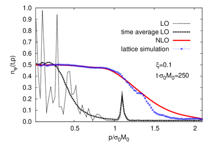
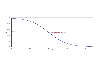
Figure 1: Left: number distribution of massless fermions produced after preheating (from Berges, Gelfand and Pruschke (2011) Berges:2010zv with kind permission). The different curves indicate the result of the inclusion of leading order (LO) and next-to-leading order (NLO) effects in the calculation. Right: Distribution functions $f(p)=[\exp(\beta(E(p)-\mu))+1]^{-1}$ (red, dashed) and $f(p)=[\exp(\alpha\beta(E(p)-\mu))+1]^{-1}$ (blue, solid) with $\alpha=40$, $\beta=0.1$, $\mu=1$ and $m=0.01$.

II.2 Deriving the effective Lagrangian

Using the expressions for the sums over the Matsubara frequencies given in the appendix we can expand the integrand to get a time-independent Lagrangian of the form

$$\mathcal{L}_{\rm eff}=\Delta^{*}(c\nabla^{2}+a)\Delta-\tfrac{1}{2}b|\Delta|^{4}.$$ (9)

The distribution (see Fig. 1) is such that low momentum modes approximately follow a thermal distribution with a large temperature related to the total energy, while high momentum states are not yet filled. To take account of the distortion from a true thermal distribution, we split the momentum integral into two parts and replace all instances of $\beta$ by $\beta/\alpha$ for $k$ satisfying $\xi=k^{2}/2m-\mu<0$ and $\alpha\beta$ for $k$ satisfying $\xi=k^{2}/2m-\mu>0$ i.e.

$$\beta(k)=\Bigg{\{}\begin{array}[]{cc}\beta/\alpha&\xi<0\\ \alpha\beta&\xi>0\end{array}$$ (10)

The effect is similar (but opposite and more extreme) to $y$-distortion in the cosmic microwave background, which occurs when Compton scattering becomes less efficient, leading to a decrease in temperature for low energy photons and a corresponding increase for high energy photons (cf. Chluba11012012 ). To model the sharp decrease in occupation number at $\xi=0$, we consider $\alpha\gg 1$. In particular, we assume

$$c_{1}\equiv\frac{\mu\beta}{2\alpha}\ll 1,\qquad\qquad c_{2}\equiv\frac{\mu\alpha\beta}{2}\gtrsim 1,$$ (11)

which are used frequently in the following sections. Thus, the effect of replacing the temperature for high momentum modes by a smaller value is that the effect of the chemical potential is no longer negligible. It should be stressed that the chemical potential term considered here is unrelated to any excess of fermions, but is merely a parameter used to describe the fermion distribution, and corresponds roughly to a value $\mu\sim k_{F}=q^{1/4}m_{\phi}$ below which the bulk of the fermion modes were created during preheating. Thermalisation in this situation would correspond to the limit $\alpha\rightarrow 1$.

Both $\mu$ and $\alpha$ have physical interpretations relating to the underlying physics. In this simplistic scenario, the end-product of the non-perturbative parametric resonance decay of the inflaton is represented by a two-parameter toy model. $\mu$, which acts as the chemical potential, is related to the inflaton mass because it is this mass scale that determines the limit in momentum space below which most of the fermions are created by parametric resonance. $\alpha$ is not related directly to the parameters in the inflaton Lagrangian, but instead depends on the physics of the decay process in a nontrivial way. It is a measure of the extent to which parametric resonance prefers low-momentum fermions, and cannot be too large (or too small) without failing to accurately represent the phenomenology of the full calculation.

So if $\alpha$ is not undetermined, what value should it take? Because $\alpha=1$ corresponds to a thermal distribution, any deviation requires that $\alpha>1$; because the distortion has been shown to be large in detailed lattice calculations, $\alpha$ must also be large to reflect this. In this toy model $\alpha$ need only be large enough to ensure that the conditions (11) are satisfied, so as to cause significant distortion of the (eventual) thermal distribution.

The key dimensionless parameter is actually $c_{2}$, not $\alpha$, as it is the degree to which $c_{2}$ exceeds unity that parameterises the importance of the chemical potential $\mu$ and controls the resulting distribution for high-momentum modes. For the chemical potential to be significant for high-momentum modes, $c_{2}\gtrsim 1$ is necessary. However, this parameter too is constrained by the requirement to capture the post-preheating physics; extremely large values ($c_{2}\gg 1$) would lead to an unnaturally sharp cutoff in the distribution function and should not be considered.

An alternative way to parameterise the distortion of the number density for high-momentum fermions would be to employ a momentum-dependent chemical potential $\mu(p)$. The form of $\mu(p)$ should satisfy the following properties:

• As thermalisation occurs, $\mu(p)\rightarrow 0$.

• $\mu(p)<0$ in order to enhance the exponential part of the Fermi-Dirac distribution.

• $|\mu(p)|$ is an increasing function of $p$, so that the suppression of the number density is enhanced for large momentum modes.

• To avoid deviations from the thermal distribution for low-momentum fermions, $p$ should not become positive for small $p$.

The effect of such a function would be closer to that of $\mu$-distortion in the CMB. An example of a function that satisfies these criteria and gives rise to the power law decay $f(p)\sim p^{-4}$ for high-momentum modes characteristic for strong turbulence (as reported in Berges:2010zv ) is

$$\mu(p)=\Bigg{\{}\begin{array}[]{cc}0,&p<p_{0}\\ \alpha[-4\beta^{-1}\log(e^{\tfrac{1}{4}\beta E(p_{0})}p/p_{0})+E(p)],&p>p_{0}\end{array}$$ (12)

where $p_{0}$ is the point at which the suppression takes effect and thermalisation occurs in the limit $\alpha\rightarrow 0$. For the remainder of this work, however, we shall use the temperature distortion prescription (10), for which the coefficients in the effective Lagrangian can be calculated analytically.

II.3 The quadratic term $a$

We expand the $\Delta^{*}\Delta$ term in (8) in gradients using

$$\frac{1}{i\omega_{n}-\xi(\bf k+i\nabla)}=\frac{1}{i\omega_{n}-\xi({\bf k})}+\frac{1}{[i\omega_{n}-\xi({\bf k})]^{2}}\frac{i\bf k\cdot\nabla}{m}+\\ +\left\{\frac{1}{[i\omega_{n}-\xi({\bf k})]^{2}}\left(\frac{-\nabla^{2}}{2m}\right)-\frac{1}{[i\omega_{n}-\xi({\bf k})]^{3}}\left(\frac{\bf k\cdot\nabla}{m}\right)^{2}\right\}+\dots$$ (13)

The term proportional to $({\bf k\cdot\nabla})\Delta^{*}\Delta$ will not contribute as we integrate over all $\bf k$. For the quadratic term we have

$$a=\frac{1}{4\pi}\int_{0}^{\sqrt{2m\mu}}\frac{dkk}{\xi}\tanh(\beta\xi/2)+\frac{1}{4\pi}\int_{\sqrt{2m\mu}}^{\infty}\frac{dkk}{\xi}\tanh(\beta\xi/2)-\frac{1}{\lambda_{0}},$$ (14)

where we have split the integral at the point $\xi=k^{2}/2m-\mu=0$. Following the standard BCS treatment, we swap the coupling constant for the binding energy of a fermion pair $\epsilon_{a}$. The two quantities are related by

$$\frac{1}{\lambda_{0}}=\tfrac{1}{2}\nu(0)\ln\left(\frac{2\epsilon_{\Lambda}}{\epsilon_{a}}\right),$$ (15)

where $\epsilon_{\Lambda}=\Lambda^{2}/2m$ ($\Lambda$ is a momentum cutoff) and $\nu(0)=m/2\pi$ is the 2d density of states per spin degree of freedom. Next, we apply the temperature prescription (10) and use the substitution

$$x=\Bigg{\{}\begin{array}[]{cc}\beta\xi/(2\alpha)&\xi<0\\ \alpha\beta\xi/2&\xi>0\end{array}$$ (16)

where $x$ is unrelated to the spacetime coordinates. This gives

$$a=\frac{1}{2}\nu(0)\left\{\int_{-c_{1}}^{0}\frac{X}{x}dx+\int_{0}^{\alpha\beta\epsilon_{\Lambda}/2}\frac{X}{x}dx+\ln\left(\frac{\epsilon_{a}}{2\epsilon_{\Lambda}}\right)\right\},$$

where we define $X=\tanh(x)$ and $c_{1}$ and $c_{2}$ are defined in (11). Since $c_{1}\ll 1$ we can neglect the contribution from the first integral. Making use of (98) with $\epsilon_{\Lambda}\rightarrow\infty$ the second integral can be rewritten

$$\int_{0}^{\alpha\beta\epsilon_{\Lambda}/2}\frac{X}{x}dx\rightarrow\ln\left(\frac{2\alpha\beta\epsilon_{\Lambda}e^{\gamma}}{\pi}\right),$$

so

$$a\simeq\tfrac{1}{2}\nu(0)\ln\left(\frac{T_{0}}{T}\right),$$ (17)

with

$$T_{0}\equiv\frac{\alpha\epsilon_{a}e^{\gamma}}{\pi}.$$ (18)

This takes the same form as the standard BCS formula but with a different transition temperature (the standard case has $T_{0}=e^{\gamma}\sqrt{2\mu\epsilon_{a}}/\pi$).

II.4 The quartic term $b$

Using (95), the quartic term is found to be

$$b=-\frac{1}{4}\int\frac{d^{2}k}{(2\pi)^{2}}\frac{1}{\xi}\frac{d}{d\xi}\left(\frac{\tanh(\beta\xi/2)}{\xi}\right).$$ (19)

Splitting the integral into two parts and using (10) and (16) gives

$$b=-\frac{\nu(0)\beta^{2}}{16}\left\{\frac{1}{\alpha^{2}}\int_{-c_{1}}^{0}\frac{dx}{x}\frac{d}{dx}\left(\frac{X}{x}\right)+\alpha^{2}\int_{0}^{\infty}\frac{dx}{x}\frac{d}{dx}\left(\frac{X}{x}\right)\right\}.$$

Neglecting the first integral as before and using (102) we find

$$b\simeq\frac{7\nu(0)\alpha^{2}\beta^{2}}{16\pi^{2}}\zeta(3).$$ (20)

II.5 The gradient term

From (13) we see that the gradient term has two contributions. Performing the sum using (96), the first can be rewritten

$$-\frac{1}{8m}\int\frac{d^{2}k}{(2\pi)^{2}}\frac{d}{d\xi}\left(\frac{\tanh(\beta\xi/2)}{\xi}\right)=-\frac{\nu(0)\alpha\beta}{16m}\left[\frac{1}{\alpha^{2}}\int_{-c_{1}}^{\infty}dx\frac{d}{dx}\left(\frac{X}{x}\right)+\int_{0}^{\infty}dx\frac{d}{dx}\left(\frac{X}{x}\right)\right].$$

Similarly, using (97), the second integral is

$$\begin{split}&-\frac{1}{32\pi m^{2}}\int_{-\beta\mu/2}^{\infty}dkk^{3}\Bigg{[}\frac{\tanh(\beta\xi/2)}{\xi^{3}}+\frac{\beta}{2}\frac{d}{d\xi}\left(\frac{\cosh(\beta\xi/2)}{\xi}\right)\Bigg{]}\\ &\quad=-\frac{\nu(0)\alpha\beta}{16m}\left[\frac{1}{\alpha^{2}}\int_{-c_{1}}^{\infty}dx\left(x+c_{1}\right)\left(\frac{X}{x^{3}}+\frac{d}{dx}\left(\frac{Y}{x}\right)\right)+\int_{0}^{\infty}dx\left(x+c_{2}\right)\left(\frac{X}{x^{3}}+\frac{d}{dx}\left(\frac{Y}{x}\right)\right)\right],\end{split}$$

where $Y\equiv\mathrm{sech}^{2}(x)$. Since $X/x^{3}+(Y/x)^{\prime}$ is smooth at $x=0$ we can let $c_{1}\rightarrow 0$ in the integrand and denominator. Combining the two parts gives the gradient term as

$$\begin{split}c&\simeq-\frac{\nu(0)\alpha\beta}{16m}\left\{\int_{0}^{\infty}dx\left(\frac{X}{x^{2}}-\frac{Y}{x}\right)+\left[\frac{X}{x}+Y\right]^{\infty}_{0}\right\},\\ &=\frac{\nu(0)\alpha\beta}{16m}.\end{split}$$ (21)

II.6 Time-dependence

To take account of the time-dependence, we must return to the quadratic term (6), using $\tilde{k}_{0}=i\omega_{n}+\partial_{\tau}=i\omega_{n}-i\omega_{\ell}$. The dynamical part of the action is then found by expanding

$$Q(i\omega_{\ell})=S_{\rm eff}^{(2)}(\vec{k}=0,k_{0}=i\omega_{n},\tilde{k}_{0}=i\omega_{n}-i\omega_{\ell})-S_{\rm eff}^{(2)}(\vec{k}=0,k_{0}=i\omega_{n},\tilde{k}_{0}=i\omega_{n}),$$

after analytic continuation to the real axis with the prescription $i\omega_{\ell}=q_{0}+i\epsilon$ SadeMelo:1993zz . The dynamical part of the effective Lagrangian is then given by Schakel:1999pa

$$\mathcal{L}_{\rm dyn}=[Q^{\prime}(i\partial_{0})-i\pi Q^{\prime\prime}(i\partial_{0})]\Delta^{*}\Delta,$$ (22)

with

$$Q^{\prime}(q_{0})=-\mathchoice{{\vbox{\hbox{$\textstyle-$ }}\kern-7.83337pt}}{{\vbox{\hbox{$\scriptstyle-$ }}\kern-5.90005pt}}{{\vbox{\hbox{$\scriptscriptstyle-$ }}\kern-4.75003pt}}{{\vbox{\hbox{$\scriptscriptstyle-$ }}\kern-4.25003pt}}\!\int_{\bf k}\frac{q_{0}\tanh(\beta\xi/2)}{2\xi(2\xi+q_{0})},\qquad Q^{\prime\prime}(q_{0})=-\int_{\bf k}\delta(2\xi+q_{0})\tanh(\tfrac{1}{2}\beta\xi),$$ (23)

where $\mathchoice{{\vbox{\hbox{$\textstyle-$ }}\kern-7.83337pt}}{{\vbox{\hbox{$\scriptstyle-$ }}\kern-5.90005pt}}{{\vbox{\hbox{$\scriptscriptstyle-$ }}\kern-4.75003pt}}{{\vbox{\hbox{$\scriptscriptstyle-$ }}\kern-4.25003pt}}\!\int$ stands for the principal part (the $Q^{\prime}$ integral has a single pole at $\xi=q_{0}/2$). Expanding the integrand about $q_{0}=0$ gives

$$\begin{split}Q^{\prime}(q_{0})&=-\frac{\nu(0)}{2}\Bigg{\{}\frac{\alpha\beta q_{0}}{4}\left[\frac{1}{\alpha^{2}}\mathchoice{{\vbox{\hbox{$\textstyle=$ }}\kern-10.83342pt}}{{\vbox{\hbox{$\scriptstyle=$ }}\kern-7.76675pt}}{{\vbox{\hbox{$\scriptscriptstyle=$ }}\kern-6.08339pt}}{{\vbox{\hbox{$\scriptscriptstyle=$ }}\kern-5.58339pt}}\!\int_{-c_{1}}^{0}\frac{X}{x^{2}}dx+\mathchoice{{\vbox{\hbox{$\textstyle=$ }}\kern-10.83342pt}}{{\vbox{\hbox{$\scriptstyle=$ }}\kern-7.76675pt}}{{\vbox{\hbox{$\scriptscriptstyle=$ }}\kern-6.08339pt}}{{\vbox{\hbox{$\scriptscriptstyle=$ }}\kern-5.58339pt}}\!\int_{0}^{\infty}\frac{X}{x^{2}}dx\right]+\mathcal{O}(q_{0}^{2})\Bigg{\}}\\ &\simeq-\frac{\nu(0)\alpha\beta q_{0}}{8}\left[\eta-\frac{\ln(c_{1})}{\alpha^{2}}\right]\\ &\simeq-\frac{\nu(0)\alpha\beta\eta q_{0}}{8},\end{split}$$ (24)

where in the second line

$$\eta\equiv 1+2\int_{0}^{\infty}XY\ln(x)dx\approx 0.7905,$$ (25)

is a constant and the principal value integrals have been evaluated using (106). In the third line, we have neglected the subdominant term $\alpha^{-2}\ln(c_{1})=\alpha^{-2}\ln(c_{2}\alpha^{-2})\ll 1$ as $\alpha$ is large. The expansion to second order in $q_{0}$ is performed in Appendix D.

The delta function in (23) picks out $\xi=-\tfrac{1}{2}q_{0}$, which, as $q_{0}\ll\mu$, is extremely close to $\xi=0$ where the temperature jumps according to the prescription (10). To avoid unphysical features arising from the treatment of the jump as a step-function we take $\beta(k)=\beta$ here, which gives

$$Q^{\prime\prime}(q_{0})=\tfrac{1}{2}\nu(0)\tanh\left(\frac{\beta q_{0}}{4}\right)\simeq\tfrac{1}{8}\nu(0)\beta q_{0}.$$ (26)

After integrating by parts, the dynamical part of the Lagrangian is then

$$\mathcal{L}_{\rm dyn}\simeq\frac{\beta\nu(0)}{8}\Delta^{*}\left(\alpha\eta i-\pi\right)\partial_{0}\Delta.$$ (27)

II.7 The effective Lagrangian

Putting these parts together gives the effective Lagrangian

$$\begin{split}\mathcal{L}_{\rm eff}=\tfrac{1}{2}\nu(0)\Bigg{\{}\Delta^{*}\Bigg{[}\ln\left(\frac{T_{0}}{T}\right)+&\frac{\beta}{4}\left(\alpha\eta i-\pi\right)\partial_{0}+\frac{\beta\alpha}{8m}\nabla^{2}\Bigg{]}\Delta-\frac{7\beta^{2}\alpha^{2}}{16\pi^{2}}\zeta(3)|\Delta|^{4}\Bigg{\}}.\end{split}$$ (28)

Considering only the potential terms, one can see from the expression for the transition temperature (18), that if $\alpha$ is large enough, $T<T_{0}$. The quadratic term in the effective potential will then be negative while the quartic term is positive; there is then a minimum at

$$|\Delta_{\rm min}|=\sqrt{\frac{16\pi^{2}}{7\alpha^{2}\beta^{2}\zeta(3)}\ln\left(\frac{\alpha\beta\epsilon_{a}e^{\gamma}}{\pi}\right)},$$ (29)

and the value of the potential at the minimum is negative

$$V(|\Delta_{\rm min}|)=-\frac{2\nu(0)\pi^{2}\ln^{2}\left(\frac{\alpha\beta\epsilon_{a}e^{\gamma}}{\pi}\right)}{7\alpha^{2}\beta^{2}\zeta(3)}.$$ (30)

Analysis of the time-independent part thus suggests that the effect of the non-thermal distribution function — implemented quantitatively with $\alpha\gg 1$ — is to give rise to a shift in the ground state of the system.

However, the form of the time-derivative terms is unusual. The interpretation of the real part of the $\Delta^{*}\partial_{0}\Delta$ term is that high energy fermion pairs can break up as in the standard BCS model with weak coupling; the imaginary part indicates that $\Delta$ has a propagating part. Time-derivative terms with complex coefficients can also occur in the weak coupling limit of the BCS-BEC crossover, as a result of a starting Lagrangian that is not particle-hole symmetric SadeMelo:1993zz . An important difference here is that the real part is subdominant. To better understand the effect of the time-derivative terms, it is necessary to repeat the analysis with a relativistic Lagrangian: this will be the subject of the following sections.

III Relativistic fermions

In this section, we apply the methods of the previous section to a 2+1 dimensional model with relativistic fermions described by the Dirac Lagrangian. Following some preliminary comments on the treatment of fermions in 2+1 dimensions, we explicitly derive the gravitational four-fermion interaction and use the result to calculate the effective Lagrangian for the pair field.

III.1 Fermions in 2+1 dimensions

To treat the case where the fermions are relativistic, our starting point must be the Dirac Lagrangian. However, in 2+1 dimensions this comes hand-in-hand with several nonintuitive features arising from the fact that in odd spacetime dimensions there are two inequivalent representations of the gamma matrices, which can be written in terms of the Pauli matrices as: $\gamma^{0}=\sigma_{3}$, $\gamma^{1}=i\sigma_{1}$, $\gamma^{2}=\pm i\sigma_{2}$. (Note that the Dirac spinors have only two components.) Following deJesusAnguianoGalicia:2005ta , we refer to the $+i\sigma_{2}$ case as the A representation and $-i\sigma_{2}$ case as the B representation.

The solutions of the Dirac equation in the A and B representations are not independent, but are related by a parity transform $\mathcal{P}$: $(\psi_{A})^{\mathcal{P}}=-i\gamma^{1}\psi_{B}e^{i\phi_{P}}$ and $(\psi_{B})^{\mathcal{P}}=-i\gamma^{1}\psi_{A}e^{-i\phi_{P}}$, where $\phi_{P}$ is a phase, which converts a spin-up particle (antiparticle) to a spin-down particle (antiparticle) and vice versa Shimizu:1984ik .

Thus in order to describe fermions with both spins, we need the (parity invariant) Lagrangian

$$\mathcal{L}=\bar{\psi}_{A}(i\not{\partial}_{A}-m)\psi_{A}+\bar{\psi}_{B}(i\not{\partial}_{A}+m)\psi_{B},$$ (31)

where the slashed notation $\not{\partial}_{A}$ in this equation indicates contraction with the $2\times 2$ gamma matrices in the A representation. This can be written in the form $\mathcal{L}=\bar{\psi}(i\not{\partial}-m)\psi$ using the four-component representation

$$\gamma^{0}=\begin{pmatrix}\sigma_{3}&0\\ \makebox[0.0pt]{$0$}&\makebox[0.0pt]{$-\sigma_{3}$}\end{pmatrix},\qquad\gamma^{1}=\begin{pmatrix}i\sigma_{1}&0\\ \makebox[0.0pt]{$0$}&\makebox[0.0pt]{$-i\sigma_{1}$}\end{pmatrix},\qquad\gamma^{2}=\begin{pmatrix}i\sigma_{2}&0\\ \makebox[0.0pt]{$0$}&\makebox[0.0pt]{$-i\sigma_{2}$}\end{pmatrix},$$ (32)

and $\psi=(\psi_{A}\ \psi_{B})^{T}$. Since there are only three gamma matrices, we have sufficient freedom to define the following matrices

$$\gamma^{3}=\begin{pmatrix}0&I\\ \makebox[0.0pt]{$I$}&\makebox[0.0pt]{$0$}\end{pmatrix},\qquad\gamma^{5}=i\begin{pmatrix}0&I\\ \makebox[0.0pt]{$-I$}&\makebox[0.0pt]{$0$}\end{pmatrix},$$ (33)

which anticommute with $\gamma^{\mu}$. From these we can define the Hermitian matrix

$$\gamma^{35}\equiv i\gamma^{3}\gamma^{5}=\left(\begin{matrix}1&0\\ \ 0\ &-1\end{matrix}\right),$$ (34)

which commutes with $\gamma^{\mu}$ and anticommutes with $\gamma^{3}$, $\gamma^{5}$.

In order to derive the equivalent Lagrangian to that used in the non-relativistic case, we shall rewrite the Lagrangian in the Nambu-Gorkov basis (cf. Deng:2006ed ) with a non-zero chemical potential $\mu$ i.e.

$$\mathcal{L}=\tfrac{1}{2}\bar{\Psi}^{NG}\begin{pmatrix}i\not{\partial}-m+\gamma^{0}\mu&0\\ 0&i\not{\partial}-m-\gamma^{0}\mu\end{pmatrix}\Psi^{NG}.$$ (35)

The Nambu-Gorkov spinor is

$$\Psi^{NG}=\begin{pmatrix}\psi\\ \psi^{c}\end{pmatrix},\qquad\bar{\Psi}^{NG}=(\bar{\psi}\quad\bar{\psi}^{c}),$$ (36)

where the superscript $c$ indicates the charge conjugate, given (up to an overall phase) by

$$\psi^{c}=C\bar{\psi}^{T},\qquad\bar{\psi}^{c}=-\psi^{T}C^{\dagger},\qquad C=\gamma^{2}e^{i\phi_{C}\gamma^{35}},$$ (37)

where $\phi_{C}$ is a phase.

III.2 Derivation of the interaction term

To derive the interaction term, we will consider minimally coupled fermions in curved space in the Vielbein-Einstein-Palatini formulism, in which the spin connection $\bar{\omega}_{\mu}{}^{I}{}_{J}$ and the vielbein $e^{\mu}_{I}$ are taken as independent variables. The Lagrangian is

$$\mathcal{L}=e\left\{\tfrac{M_{\mathrm{pl}}}{2}e_{I}^{\mu}e^{\nu J}R_{\mu\nu}{}^{I}{}_{J}+\tfrac{i}{2}\left[\bar{\psi}e^{\mu}_{I}\nabla_{\mu}\psi-(\nabla_{\mu}\bar{\psi})e^{\mu}_{I}\gamma^{I}\psi\right]-m\bar{\psi}\psi\right\},$$ (38)

where $e=|\det(e^{I}_{\mu})|$ and $M_{\mathrm{pl}}=(8\pi G_{3})^{-1}$ is the reduced Planck mass in three spacetime dimensions. $R_{\mu\nu}{}^{I}{}_{J}$ and the covariant derivatives of the fermions are given in terms of the spin connection by

$$R_{\mu\nu}{}^{I}{}_{J}=\partial_{\nu}\bar{\omega}_{\mu}{}^{I}{}_{J}-\partial_{\mu}\bar{\omega}_{\nu}{}^{I}{}_{J}+\bar{\omega}_{\nu}{}^{I}{}_{K}\bar{\omega}_{\mu}{}^{K}{}_{J}-\bar{\omega}_{\mu}{}^{I}{}_{K}\bar{\omega}_{\nu}{}^{K}{}_{J}.$$ (39)

and

$$\nabla_{\mu}\psi=\partial_{\mu}\psi+\tfrac{1}{4}\bar{\omega}_{\mu IJ}\gamma^{[I}\gamma^{J]}\psi,\qquad\nabla_{\mu}\bar{\psi}=\partial_{\mu}\psi-\tfrac{1}{4}\bar{\psi}\bar{\omega}_{\mu IJ}\gamma^{[I}\gamma^{J]}.$$ (40)

The spin connection can be decomposed into the symmetric Levi-Civita spin-connection $\omega_{\mu}{}^{I}{}_{J}$ (which is torsionfree and metric compatible i.e. $\nabla_{\mu}\eta_{IJ}=0$) and an antisymmetric part $D_{\mu}{}^{I}{}_{J}$ as

$$\bar{\omega}_{\mu}{}^{I}{}_{J}=\omega_{\mu}{}^{I}{}_{J}+D_{\mu}{}^{I}{}_{J},$$

so that the Lagrangian can be be rewritten as $\mathcal{L}=\mathcal{L}_{LC}+\mathcal{L}_{\rm torsion}$, where $\mathcal{L}_{LC}$ takes the same form as (38), but with covariant derivatives and $R_{\mu\nu}{}^{I}{}_{J}$ given purely in terms of the Levi-Civita spin connection $\omega_{\mu}{}^{I}{}_{J}$. The second term $\mathcal{L}_{\rm torsion}$ contains the torsion-dependent parts of the original gravitational and fermion Lagrangians and is given explicitly by

$$\mathcal{L}_{\rm torsion}=e\left\{\frac{M_{\mathrm{pl}}}{2}e_{I}^{\mu}e^{\nu J}\left(D_{\nu}{}^{I}{}_{K}D_{\mu}{}^{K}{}_{J}-D_{\mu}{}^{I}{}_{K}D_{\nu}{}^{K}{}_{J}\right)+D_{\mu IJ}A^{\mu IJ}\right\},$$ (41)

(plus a total divergence) with

$$A^{\mu IJ}\equiv\tfrac{i}{8}e^{\mu}_{K}\bar{\psi}\left\{\gamma^{[I}\gamma^{J]},\gamma^{K}\right\}\psi=\tfrac{1}{4}e^{\mu}_{K}\epsilon^{IJK}(\bar{\psi}\gamma^{35}\psi).$$ (42)

In the second equality of (42) we have used the identity $\left\{\gamma^{[I}\gamma^{J]},\gamma^{K}\right\}=2\epsilon^{IJK}\gamma^{3}\gamma^{5}=-2i\epsilon^{IJK}\gamma^{35}$. We can now find an explicit expression for the antisymmetric part of the spin-connection by considering the equation of motion obtained from $\mathcal{L}_{\rm torsion}$ Dadhich:2010xa . Defining the tensors

$$E_{\mu}{}^{\alpha}{}_{\beta}\equiv e^{\alpha}_{I}e^{K}_{\beta}D_{\mu}{}^{I}{}_{K},\qquad\text{and}\qquad A^{\mu\rho\sigma}\equiv e^{\rho}_{K}e^{\sigma}_{L}A^{\mu KL},$$ (43)

the Lagrangian can be written

$$\mathcal{L}_{\rm torsion}=eE^{\alpha\beta\gamma}\left[\tfrac{1}{2}M_{\mathrm{pl}}\left(E_{\beta\gamma\alpha}-g_{\alpha\gamma}E^{\mu}{}_{\mu\beta}\right)+A_{\alpha\beta\gamma}\right].$$ (44)

Varying with respect to $E^{\alpha\beta\gamma}$ yields

$$E_{\beta\gamma\alpha}+E_{\gamma\alpha\beta}-g_{\alpha\gamma}E^{\mu}{}_{\mu\beta}-g_{\alpha\beta}E^{\mu}{}_{\gamma\mu}=\tilde{A}_{\alpha\beta\gamma},$$ (45)

where $\tilde{A}_{\alpha\beta\gamma}=-\tfrac{2}{M_{\mathrm{pl}}}A_{\alpha\beta\gamma}$. $E^{\alpha\beta\gamma}$ has three independent traces: $c_{1}=E_{\gamma\rho}{}^{\rho}$, $c_{2}=E_{\rho\gamma}{}^{\rho}$ and $c_{3}=E_{\rho}{}^{\rho}{}_{\gamma}$. Substituting these into (45) and contracting indices with $g^{\alpha\gamma}$ and $g^{\gamma\beta}$ yields the relation

$$c_{2}=c_{3}+2\tilde{A}^{\alpha}{}_{\beta\alpha},$$

so (45) can be rewritten in terms of $\tilde{A}_{\alpha\beta\gamma}$ and an arbitrary vector $U_{\gamma}=c_{3}$ as

$$E_{\beta\gamma\alpha}+E_{\gamma\alpha\beta}=\tilde{A}_{\alpha\beta\gamma}+2g_{\alpha\beta}\tilde{A}^{\rho}{}_{\gamma\rho}+g_{\alpha\gamma}U_{\beta}+g_{\alpha\beta}U_{\gamma}.$$

Cyclically permuting indices gives two further equations, which combine to give

$$\begin{split}E_{\alpha\beta\gamma}&=\tfrac{1}{2}(\tilde{A}_{\gamma\alpha\beta}+\tilde{A}_{\beta\gamma\alpha}-\tilde{A}_{\alpha\beta\gamma})+(g_{\beta\gamma}\tilde{A}^{\rho}{}_{\alpha\rho}+g_{\alpha\gamma}\tilde{A}^{\rho}{}_{\beta\rho}-g_{\alpha\beta}\tilde{A}^{\rho}{}_{\gamma\rho})+g_{\beta\gamma}U_{\alpha},\\ &=\tfrac{1}{2}\tilde{A}_{\alpha\beta\gamma}+g_{\beta\gamma}U_{\alpha},\end{split}$$ (46)

where in the second line we have used the fact that $\tilde{A}_{\alpha\beta\gamma}$ is totally antisymmetric, as can been seen from (42). Substituting this back into the Lagrangian (44) gives

$$\mathcal{L}_{\rm torsion}=-\frac{e}{2M_{\mathrm{pl}}}A^{\alpha\beta\gamma}A_{\alpha\beta\gamma},$$ (47)

where the symmetric part vanishes due to the antisymmetry of $A^{\alpha\beta\gamma}$; as it should, since it is a gauge artifact Dadhich:2010xa . Substituting the definition of $A^{\alpha\beta\gamma}$ in (42) and using the identity $\epsilon_{IJK}\epsilon^{IJK}=6$ yields the interaction term

$$\mathcal{L}_{\rm torsion}=-\frac{3e}{16M_{\mathrm{pl}}}(\bar{\psi}\gamma^{35}\psi)^{2}.$$ (48)

To make contact with the fermion Lagrangian in the Nambu-Gorkov basis (35) we shall rewrite $\mathcal{L}_{\rm torsion}$ in terms of the charge-conjugated fields (37) using the Fierz identities given in Appendix B. Applying (114) gives

$$\mathcal{L}_{\rm torsion}=\frac{\lambda_{0}}{2}\left[(\bar{\psi}\psi^{c})(\bar{\psi}^{c}\psi)+(\bar{\psi}\gamma^{35}\psi^{c})(\bar{\psi}^{c}\gamma^{35}\psi)+\tilde{\Phi}^{\dagger}\tilde{\Phi}+\tilde{\Phi}^{\dagger}_{\mu}\tilde{\Phi}^{\mu}\right],$$ (49)

where

$$\lambda_{0}=\frac{3}{32M_{\mathrm{pl}}}=\frac{3}{4}\pi G_{3},$$ (50)

and the doublets $\tilde{\Phi}$ and $\tilde{\Phi}^{\mu}$ are defined in (115). In what follows, for simplicity we shall focus on the effect of the scalar and $\gamma^{35}$ interactions.

III.3 Integrating out the fermions

Following the procedure used in the non-relativistic case, we remove the four-fermion interaction by inserting the following terms in the Lagrangian,

$$-\frac{1}{2\lambda_{0}}\left\{[\Delta_{1}-\lambda_{0}\bar{\psi}^{c}\psi]^{\dagger}[\Delta_{1}-\lambda_{0}\bar{\psi}^{c}\psi]+[\Delta_{2}-\lambda_{0}\bar{\psi}^{c}\gamma^{35}\psi]^{\dagger}[\Delta_{2}-\lambda_{0}\bar{\psi}^{c}\gamma^{35}\psi]\right\},$$

which correspond to multiplying the path integral by a Gaussian integral in the auxiliary fields, and thus do not affect the equations of motion. Variation with respect to $\Delta_{1}^{\dagger}$ and $\Delta_{2}^{\dagger}$ show that $\Delta_{1}$ and $\Delta_{2}$ describe fermion pairs coupled in the scalar and $\gamma^{35}$ channels

$$\Delta_{1}=\lambda_{0}\bar{\psi}^{c}\psi,\qquad\Delta_{2}=\lambda_{0}\bar{\psi}^{c}\gamma^{35}\psi.$$ (51)

Rather than work directly with $\Delta_{1}$ and $\Delta_{2}$, we redefine as follows

$$\Delta_{A}=\tfrac{1}{2}(\Delta_{1}+\Delta_{2}),\qquad\Delta_{B}=\tfrac{1}{2}(\Delta_{1}-\Delta_{2}),$$ (52)

so the interaction Lagrangian is

$$\mathcal{L}_{\text{int}}=\tfrac{1}{2}\bar{\Psi}^{NG}\begin{pmatrix}0&0&\Delta_{A}&0\\ 0&0&0&\Delta_{B}\\ \Delta_{A}^{\dagger}&0&0&0\\ 0&\Delta_{B}^{\dagger}&0&0\end{pmatrix}\Psi^{NG}-\frac{1}{\lambda_{0}}(|\Delta_{A}|^{2}+|\Delta_{B}|^{2}),$$ (53)

where each entry indicates a $2\times 2$ block. The advantage of this is that the complete Lagrangian may be split into two parts, composed of $\psi_{A}$ and $\psi_{B}$ spinors respectively, as

$$\mathcal{L}=\mathcal{L}_{A}+\mathcal{L}_{B}=(\mathcal{L}_{A}^{\psi}+\mathcal{L}_{A}^{\text{tree}})+(\mathcal{L}_{B}^{\psi}+\mathcal{L}_{B}^{\text{tree}})$$

with

$$\mathcal{L}_{A}^{\psi} = \tfrac{1}{2}\bar{\Psi}^{NG}_{A}\begin{pmatrix}i\not{\partial}-m+\gamma^{0}\mu&\Delta_{A}\\ \Delta_{A}^{\dagger}&i\not{\partial}-m-\gamma^{0}\mu\end{pmatrix}\Psi^{NG}_{A},$$ (54)

$$\mathcal{L}_{B}^{\psi} = \tfrac{1}{2}\bar{\Psi}^{NG}_{B}\begin{pmatrix}i\not{\partial}+m+\gamma^{0}\mu&-\Delta_{B}\\ -\Delta_{B}^{\dagger}&i\not{\partial}+m-\gamma^{0}\mu\end{pmatrix}\Psi^{NG}_{B},$$ (55)

and

$$\mathcal{L}_{A}^{\text{tree}}=-\frac{1}{\lambda_{0}}|\Delta_{A}|^{2},\qquad\mathcal{L}_{B}^{\text{tree}}=-\frac{1}{\lambda_{0}}|\Delta_{B}|^{2}.$$ (56)

IV The massless case

In this section, we specialise to the extreme case of massless fermions. For simplicity, and because we consider only the the very short time-scales relevant for the preheating process, we do not consider the effect of a curved background. Preheating occurs when the homogeneous zero mode of the inflaton field is exhibiting oscillations about the minimum of its potential, so that the dominant effect of including spacetime curvature is to introduce an additional friction term that damps the oscillations. Whilst this does have an effect on the process of parametric resonance used to produce the fermions, on very small timescales, one can treat the background as constant.

In this case, the covariant derivatives in the Dirac Lagrangian (taken with the Levi-Civita spin connection) reduce to partial derivatives. Here, as in (31), the $2\times 2$ gamma matrices are $\gamma^{0}=\sigma_{3}$, $\gamma^{1}=i\sigma_{1}$ and $\gamma^{2}=i\sigma_{2}$.

Considering only the $A$ parts, we can integrate out the fermions to get

$$Z=\int D\Delta_{A}^{\dagger}D\Delta_{A}\exp\left(iS_{\rm eff}-\frac{i}{\lambda_{0}}\int_{x}|\Delta_{A}|^{2}\right),$$ (57)

where $S_{\rm eff}$ is the one-loop effective action

$$S_{\rm eff}=-i\text{Tr}\ln[K(p,x)]=-i\text{tr}\int_{x}\int_{k}e^{ik\cdot x}\ln[K(p,x)]e^{-ik\cdot x}.$$ (58)

Anticipating the derivative expansion Schakel:1999pa , we write $K(p,x)$ as

$$K(p,x)=G_{0}^{-1}\left[I-G_{0}\left(\begin{smallmatrix}0&-\Delta_{A}\\ -\Delta_{A}^{\dagger}&0\end{smallmatrix}\right)\right],$$ (59)

with

$$G_{0}=\begin{pmatrix}G_{+}&0\\ 0&G_{-}\end{pmatrix},\qquad G_{\pm}=\frac{1}{(p_{0}\pm\mu)^{2}-p^{2}}\begin{pmatrix}p_{0}\pm\mu&-ip_{1}-p_{2}\\ -ip_{1}+p_{2}&-p_{0}\mp\mu\end{pmatrix}.$$ (60)

Here $p=\sqrt{p_{1}^{2}+p_{2}^{2}}$. Dropping the $\log G_{0}^{-1}$ term, which is independent of $\Delta_{A}$ and does not contribute to the effective action, we can expand as

$$S_{\rm eff}=\sum_{\ell=1}^{\infty}S_{\rm eff}^{(\ell)}=i\text{Tr}\sum_{\ell=1}^{\infty}\frac{(-1)^{\ell}}{\ell}\begin{pmatrix}0&G_{+}\Delta_{A}\\ G_{-}\Delta_{A}^{\dagger}&0\end{pmatrix}^{\ell}.$$ (61)

As in the non-relativistic case only the even powers give a non-zero contribution. For $\ell=2$ we get

$$S_{\rm eff}^{(2)}=i\text{Tr}\left\{\frac{(k_{0}-\mu)(\tilde{k}_{0}+\mu)-k_{1}\tilde{k}_{1}-k_{2}\tilde{k}_{2}}{[(k_{0}-\mu)^{2}-k^{2}][(\tilde{k}_{0}+\mu)^{2}-\tilde{k}^{2}]}\Delta_{A}^{\dagger}\Delta_{A}+\frac{(k_{0}+\mu)(\tilde{k}_{0}-\mu)-k_{1}\tilde{k}_{1}-k_{2}\tilde{k}_{2}}{[(k_{0}+\mu)^{2}-k^{2}][(\tilde{k}_{0}-\mu)^{2}-\tilde{k}^{2}]}\Delta_{A}\Delta_{A}^{\dagger}\right\},$$ (62)

where $\tilde{k}_{\mu}=(k_{0}-i\partial_{0},k_{i}+i\nabla_{i})$. An important subtlety here is that the derivatives here act only on the next object on their right, meaning that after expanding in $\tilde{k}_{\mu}$, the first derivatives in the first term in (62) pick up a minus sign from integration by parts when the term is expressed in the form $\propto\Delta_{A}^{\dagger}\partial_{\mu}\Delta_{A}$. We include the quartic terms without derivatives, so $p_{\mu}$ can be treated as a c-number, giving

$$S_{\rm eff}^{(4)}=\frac{i}{2}\text{Tr}\left\{\frac{1}{[k_{0}^{2}-\xi(k)]^{2}}+\frac{1}{[k_{0}^{2}-\bar{\xi}(k)]^{2}}\right\}|\Delta_{A}|^{4}.$$ (63)

Here we have introduced the useful notation

$$\xi(k)=k-\mu,\qquad\qquad\bar{\xi}(k)=k+\mu.$$ (64)

The time-independent part of the Euclidean action is then

$$S_{\rm eff}^{E}=\int_{0}^{\beta}d\tau\int_{\bf x}\int_{\bf k}\beta^{-1}\sum_{n}\bigg{[}\bigg{(}M_{Q_{1}}\nabla^{2}+M_{Q_{2}}(\vec{k}\cdot\vec{\nabla})^{2}-\frac{1}{\omega_{n}^{2}+\xi^{2}}-\frac{1}{\omega_{n}^{2}+\bar{\xi}^{2}}\bigg{)}|\Delta_{A}|^{2}+\\ +\frac{1}{2}\left(\frac{1}{[\omega_{n}^{2}+\xi]^{2}}+\frac{1}{[\omega_{n}^{2}+\bar{\xi}]^{2}}\right)|\Delta_{A}|^{4}\bigg{]},$$ (65)

where the coefficients $M_{L}$, $M_{Q_{1}}$ and $M_{Q_{2}}$ are defined in Appendix C. We have not included the linear term (proportional to $i{\bf k\cdot\nabla}$) since it vanishes when we integrate over all $\bf k$.

IV.1 Deriving the effective Lagrangian

In deriving the effective Lagrangian for $\Delta_{A}$, we proceed along the same lines as in Sec. II.2, applying the temperature prescription (10) with $\xi=k-\mu$. Each of the terms in the Lagrangian (9) can be split into terms involving only $\xi$ and $\bar{\xi}$, as can already be seen in (65). The latter, involving the combination $k+\mu$, arise from the antifermions (cf. OHSAKU_2+1 ; Nishida:2005ds ; He:2007kd ) and, as we shall see, represent only subdominant contributions.

IV.1.1 The quadratic term $a$

Using the Matsubura sums in Appendix A, the quadratic term is

$$\begin{split}a&=\int\frac{d^{2}k}{(2\pi)^{2}}\left[\frac{\tanh(\tfrac{1}{2}\beta\xi)}{\xi}+\frac{\tanh(\tfrac{1}{2}\beta\bar{\xi})}{\bar{\xi}}\right]-\frac{1}{\lambda_{0}},\\ &\equiv a_{\xi}+a_{\bar{\xi}}-\frac{1}{\lambda_{0}}.\end{split}$$ (66)

We can treat the $\xi$ and $\bar{\xi}$ parts separately. Starting with the first term, we apply the temperature prescription (10) to get

$$\begin{split}a_{\xi}&=\frac{1}{4\pi}\left\{\int_{0}^{\mu}dkk\frac{\tanh(\tfrac{\beta}{2\alpha}\xi)}{\xi}+\int_{\mu}^{\Lambda}dkk\frac{\tanh(\tfrac{\alpha\beta}{2}\xi)}{\xi}\right\},\\ &=\frac{1}{4\pi}\left\{\frac{2\alpha}{\beta}\int_{-c_{1}}^{0}dx(x+c_{1})\frac{X}{x}+\frac{2}{\alpha\beta}\int_{0}^{\alpha\beta\Lambda/2}dx(x+c_{2})\frac{X}{x}\right\},\end{split}$$ (67)

where $c_{1}$ and $c_{2}$ are defined in (11), $\Lambda$ is a UV cutoff, and we have used $x=\beta\xi/(2\alpha)$ in the first integral and $x=\alpha\beta\xi/2$ in the second. In the limit $c_{1}\rightarrow 0$ the first integral can be neglected. Thus

$$\begin{split}a_{\xi}&\simeq\frac{1}{2\pi\alpha\beta}\left[\ln(\cosh(\alpha\beta\Lambda/2))+c_{2}\ln\left(\frac{2\alpha\beta\Lambda e^{\gamma}}{\pi}\right)\right],\\ &\simeq\frac{\Lambda}{4\pi}+\frac{1}{2\pi\alpha\beta}\left[c_{2}\ln\left(\frac{2\alpha\beta\Lambda e^{\gamma}}{\pi}\right)-\ln 2\right].\end{split}$$ (68)

Returning to the $\bar{\xi}$ integral, we proceed in a similar fashion and split the integral at $k=\mu$. Using the substitutions $x=\beta\bar{\xi}/(2\alpha)$ and $x=\alpha\beta\bar{\xi}/2$ and the definition (64) we get

$$\begin{split}a_{\bar{\xi}}&=\frac{1}{4\pi}\left\{\frac{2\alpha}{\beta}\int_{c_{1}}^{2c_{1}}dx(x-c_{1})\frac{X}{x}+\frac{2}{\alpha\beta}\int_{2c_{2}}^{\alpha\beta\Lambda/2}dx(x-c_{2})\frac{X}{x}\right\},\\ &\simeq\frac{\Lambda}{4\pi}+\frac{1}{2\pi\alpha\beta}\left[-c_{2}\ln\left(\frac{2\alpha\beta\Lambda e^{\gamma}}{\pi}\right)-\ln 2-\int_{0}^{2c_{2}}dx(x-c_{2})\frac{X}{x}\right],\\ &\simeq\frac{\Lambda}{4\pi}+\frac{1}{2\pi\alpha\beta}\left[-c_{2}\ln\left(\frac{2\alpha\beta\Lambda e^{\gamma}}{\pi}\right)+c_{2}\ln\left(\frac{4e^{\gamma-2}c_{2}}{\pi}\right)\right],\end{split}$$ (69)

where, as before, we have neglected the first integral in the limit $c_{1}\rightarrow 0$. In the last line we used the fact that $c_{2}\gtrsim 1$ to simplify the integral using $\int_{0}^{2c_{2}}Xdx\simeq 2c_{2}-\ln 2$ and (98). The quadratic function can then be written

$$a\simeq\frac{\Lambda}{2\pi}+\frac{1}{2\pi\alpha\beta}\left[c_{2}\ln\left(\frac{4e^{\gamma-2}c_{2}}{\pi}\right)-\ln 2\right]-\frac{1}{\lambda_{0}}.$$ (70)

In the nonrelativistic calculation, the explicit dependence on the cutoff was removed by expressing the coupling constant $\lambda_{0}$ in terms of the binding energy in vacuum, obtained by solving the Schrödinger equation for a fermionic pair in vacuum. Since in this case we deal with massless fermions, this cannot be done. Nevertheless, it is instructive to consider the equivalent problem for relativistic bound states using the instantaneous Bethe-Salpeter equations. For spinless fermion-fermion bound states with a scalar interaction, the scalar part of the reduced wavefunction $\Psi_{S}$ satisfies Suttorp:1979sd

$$\frac{E}{k^{2}}(E^{2}-\epsilon_{B}^{2})\Psi_{S}(k)=\int_{\vec{k}^{\prime}}V_{S}\Psi_{S}(\vec{k}^{\prime}),$$ (71)

where $E=k^{2}+m^{2}$, and the bound state has a mass $2\epsilon_{B}<2m$. As in the nonrelativistic case, we consider for simplicity an attractive scalar contact interaction $\lambda_{0}\delta(\vec{x})$ (cf. Schakel:1999pa ) which gives

$$\frac{1}{\lambda_{0}}=\frac{1}{2\pi}\int_{0}^{\Lambda}dk\frac{k^{3}}{\sqrt{m^{2}+k^{2}}(m^{2}+k^{2}-\epsilon_{B}^{2})}\simeq\frac{\Lambda}{2\pi}-\frac{m}{2\pi}\left(1+\frac{1-B^{2}}{B}{\rm arctanh}(B)\right)+\mathcal{O}(\Lambda^{-1}),$$ (72)

where $B=\epsilon_{B}/m$. In the limit of small $m$ with $B$ finite we see the same dependence on the cutoff as exhibited in (70), with corrections of $\mathcal{O}(m)$. This suggests that (for $c_{2}\gtrsim 1$) the leading term in $a$ is the logarithm and the coefficient is approximately given by

$$a\approx\frac{c_{2}}{2\pi\alpha\beta}\ln\left(\frac{4e^{\gamma-2}c_{2}}{\pi}\right).$$ (73)

We postpone a discussion on the validity of this approach until Sec. V.

IV.1.2 The quartic term $b$

Using (95), the quartic term is

$$b=-\frac{1}{4}\int\frac{d^{2}k}{(2\pi)^{2}}\left[\frac{1}{\xi}\frac{d}{d\xi}\left(\frac{\tanh(\tfrac{1}{2}\beta\xi)}{\xi}\right)+\frac{1}{\bar{\xi}}\frac{d}{d\bar{\xi}}\left(\frac{\tanh(\tfrac{1}{2}\beta\bar{\xi})}{\xi}\right)\right].$$ (74)

Repeating the steps taken in the evaluation of $a$, we obtain

$$\begin{split}b&=-\frac{\alpha\beta}{16\pi}\left\{\int_{0}^{\infty}dx\left(\frac{x+c_{2}}{x}\right)\frac{d}{dx}\left(\frac{X}{x}\right)+\int_{2c_{2}}^{\infty}dx\left(\frac{x-c_{2}}{x}\right)\frac{d}{dx}\left(\frac{X}{x}\right)\right\},\\ &=\frac{\alpha\beta}{16\pi}\left\{1+\frac{\tanh(2c_{2})}{2c_{2}}-c_{2}\int_{0}^{2c_{2}}\frac{dx}{x}\frac{d}{dx}\left(\frac{X}{x}\right)\right\},\\ &=\frac{\alpha\beta}{16\pi}\left\{1+\frac{\tanh(2c_{2})}{8c_{2}}+\frac{\mathrm{sech}^{2}(2c_{2})}{4}+c_{2}\int_{0}^{2c_{2}}dx\frac{XY}{x}\right\},\\ &\approx\frac{\alpha\beta}{16\pi}\left\{1+\frac{7\zeta(3)}{\pi^{2}}c_{2}\right\},\end{split}$$ (75)

where in the third line we have used (101). In the fourth line, we have neglected the subdominant $\tanh$ term (which is $<0.12$ for $c_{2}>1$) and used (100) and (107).

IV.1.3 The gradient term

From (65) it can be seen that there are two contributions to the coefficient of the gradient term in the Lagrangian. (The linear term $M_{L}$ need not be considered as it vanishes when we perform the angular integral.) Taking account of the factor of $\tfrac{1}{2}$ arising from the $\cos^{2}\theta$ in the scalar product, the coefficient is

$$M=-\sum_{n}\left[M_{Q_{1}}+\tfrac{1}{2}k^{2}M_{Q_{2}}\right]=M_{\xi}+M_{\bar{\xi}}\ ,$$

where the coefficients $M_{Q_{1}}$ and $M_{Q_{2}}$ are given by (116) and

$$\begin{split}M_{\xi}&=\frac{1}{64\pi}\int_{0}^{\infty}dk\left\{\frac{\beta^{2}k}{\xi}\mathrm{sech}^{2}(\tfrac{1}{2}\beta\xi)\tanh(\tfrac{1}{2}\beta\xi)+\beta\mu\frac{\mathrm{sech}^{2}(\tfrac{1}{2}\beta\xi)}{\xi^{2}}+\frac{2(\xi-\mu)}{\mu\xi^{3}}\tanh(\tfrac{1}{2}\beta\xi)\right\},\\ &=\frac{\beta}{64\pi\alpha}\int_{-c_{1}}^{0}dx\tilde{M}_{\xi}+\frac{\alpha\beta}{64\pi}\int_{0}^{\infty}dx\tilde{M}_{\xi}.\end{split}$$ (76)

In the first line we have evaluated the Matsubura sums using (117) and in the second applied the prescription (10). Similarly, the second term is

$$M_{\bar{\xi}}=\frac{\beta}{64\pi\alpha}\int_{c_{1}}^{2c_{1}}dx\tilde{M}_{\bar{\xi}}+\frac{\alpha\beta}{64\pi}\int_{2c_{2}}^{\infty}dx\tilde{M}_{\bar{\xi}}\ ,$$ (77)

where the integrands are given by

$$\tilde{M}_{\xi} =\frac{2(x+c_{2})}{x}XY+c_{2}\frac{Y}{x^{2}}+\left(\frac{x^{2}-c_{2}^{2}}{c_{2}}\right)\frac{X}{x^{3}},$$ (78a)

$$\tilde{M}_{\bar{\xi}} =\frac{2(x-c_{2})}{x}XY-c_{2}\frac{Y}{x^{2}}-\left(\frac{x^{2}-c_{2}^{2}}{c_{2}}\right)\frac{X}{x^{3}},$$ (78b)

and we have evaluated the Matsubura sums using (117). Neglecting the $c_{1}$ integrals we find

$$\begin{split}M&=\frac{\alpha\beta}{64\pi}\left[2\hskip 1.00006pt\mathrm{sech}^{2}(2c_{2})+\int_{0}^{2c_{2}}dx\tilde{M}_{\xi}\right],\\ &=\frac{\alpha\beta}{64\pi}\left[1+\frac{1}{8c_{2}}\left[\tanh(2c)+6\mathrm{sech}^{2}(2c_{2})\right]+\frac{1}{c_{2}}\int_{0}^{2c_{2}}dx(c_{2}^{2}Y+1)\frac{X}{x}\right],\end{split}$$ (79)

where in the second line we have used (103). We can make use of use of (98) and (100) to obtain the following approximation

$$M\simeq\frac{\alpha\beta}{64\pi}\left[1+\frac{7\zeta(3)}{\pi^{2}}c_{2}+\frac{1}{c_{2}}\ln\left(\frac{8c_{2}e^{\gamma}}{\pi}\right)\right],$$ (80)

which is valid for $c_{2}\gtrsim 1$.

IV.1.4 Time-dependence

Following the procedure discussed in Sec. II.6, the time-dependent part of the effective Lagrangian is

$$\mathcal{L}_{\rm dyn}=[Q_{(+)}^{\prime}(i\partial_{0})-i\pi Q_{(+)}^{\prime\prime}(i\partial_{0})]\Delta^{\dagger}_{A}\Delta_{A}+[Q_{(-)}^{\prime}(i\partial_{0})-i\pi Q_{(-)}^{\prime\prime}(i\partial_{0})]\Delta_{A}\Delta^{\dagger}_{A},$$ (81)

with

$$Q_{(\pm)}^{\prime}(q_{0}) =-\frac{q_{0}}{4}\left(\mathchoice{{\vbox{\hbox{$\textstyle-$ }}\kern-7.83337pt}}{{\vbox{\hbox{$\scriptstyle-$ }}\kern-5.90005pt}}{{\vbox{\hbox{$\scriptscriptstyle-$ }}\kern-4.75003pt}}{{\vbox{\hbox{$\scriptscriptstyle-$ }}\kern-4.25003pt}}\!\int_{\vec{k}}\frac{\tanh(\tfrac{1}{2}\beta\xi)}{\xi(q_{0}\pm 2\xi)}+\mathchoice{{\vbox{\hbox{$\textstyle-$ }}\kern-7.83337pt}}{{\vbox{\hbox{$\scriptstyle-$ }}\kern-5.90005pt}}{{\vbox{\hbox{$\scriptscriptstyle-$ }}\kern-4.75003pt}}{{\vbox{\hbox{$\scriptscriptstyle-$ }}\kern-4.25003pt}}\!\int_{\vec{k}}\frac{\tanh(\tfrac{1}{2}\beta\bar{\xi})}{\bar{\xi}(q_{0}\mp 2\bar{\xi})}\right),$$ (82a)

$$Q_{(\pm)}^{\prime\prime}(q_{0}) =\mp\tfrac{1}{2}\int_{\vec{k}}\left[\tanh(\tfrac{1}{2}\beta\xi)\delta(q_{0}\pm 2\xi)-\tanh(\tfrac{1}{2}\beta\bar{\xi})\delta(q_{0}\mp 2\bar{\xi})\right].$$ (82b)

The barred integral indicates that the principal part should be computed. Expanding (82a) in $q_{0}$ to first order and applying the prescription (10) gives

$$\begin{split}Q_{(-)}^{\prime}(q_{0})=-Q_{(+)}^{\prime}&=\frac{q_{0}}{8}\left[\mathchoice{{\vbox{\hbox{$\textstyle=$ }}\kern-10.83342pt}}{{\vbox{\hbox{$\scriptstyle=$ }}\kern-7.76675pt}}{{\vbox{\hbox{$\scriptscriptstyle=$ }}\kern-6.08339pt}}{{\vbox{\hbox{$\scriptscriptstyle=$ }}\kern-5.58339pt}}\!\int_{\vec{k}}\frac{\tanh(\tfrac{1}{2}\beta\xi)}{\xi^{2}}-\mathchoice{{\vbox{\hbox{$\textstyle=$ }}\kern-10.83342pt}}{{\vbox{\hbox{$\scriptstyle=$ }}\kern-7.76675pt}}{{\vbox{\hbox{$\scriptscriptstyle=$ }}\kern-6.08339pt}}{{\vbox{\hbox{$\scriptscriptstyle=$ }}\kern-5.58339pt}}\!\int_{\vec{k}}\frac{\tanh(\tfrac{1}{2}\beta\bar{\xi})}{\bar{\xi}^{2}}\right],\\ &=\frac{q_{0}}{16\pi}\bigg{[}\mathchoice{{\vbox{\hbox{$\textstyle=$ }}\kern-10.83342pt}}{{\vbox{\hbox{$\scriptstyle=$ }}\kern-7.76675pt}}{{\vbox{\hbox{$\scriptscriptstyle=$ }}\kern-6.08339pt}}{{\vbox{\hbox{$\scriptscriptstyle=$ }}\kern-5.58339pt}}\!\int_{-c_{1}}^{0}\left(\frac{x+c_{1}}{x}\right)Xdx-\int_{c_{1}}^{2c_{1}}\left(\frac{x-c_{1}}{x}\right)Xdx\ +\\ &\qquad\qquad\qquad\qquad+\mathchoice{{\vbox{\hbox{$\textstyle=$ }}\kern-10.83342pt}}{{\vbox{\hbox{$\scriptstyle=$ }}\kern-7.76675pt}}{{\vbox{\hbox{$\scriptscriptstyle=$ }}\kern-6.08339pt}}{{\vbox{\hbox{$\scriptscriptstyle=$ }}\kern-5.58339pt}}\!\int_{0}^{\infty}\frac{X}{x^{2}}dx+\int_{0}^{2c_{2}}\frac{X}{x}dx+c_{2}\int_{2c_{2}}^{\infty}\frac{X}{x^{2}}dx\bigg{]},\end{split}$$ (83)

where in the second line we have applied the prescription (10) and converted to $x$ as before, combining integrals where possible. Since, using (106b) we have

$$c_{1}\mathchoice{{\vbox{\hbox{$\textstyle=$ }}\kern-10.83342pt}}{{\vbox{\hbox{$\scriptstyle=$ }}\kern-7.76675pt}}{{\vbox{\hbox{$\scriptscriptstyle=$ }}\kern-6.08339pt}}{{\vbox{\hbox{$\scriptscriptstyle=$ }}\kern-5.58339pt}}\!\int_{-c_{1}}^{0}\frac{X}{x^{2}}dx\approx-c_{1}\ln(c_{1}),$$

and the other $c_{1}$ integrals are $\mathcal{O}(c_{1})$, we can neglect their contribution. Using (98), (106a) and (108), when $c_{2}\gtrsim 1$ we get

$$Q_{(-)}^{\prime}(q_{0})=-Q_{(+)}^{\prime}\simeq\frac{q_{0}}{16\pi}\left[\eta c_{2}+\ln\left(\frac{8e^{\gamma+1/2}c_{2}}{\pi}\right)\right].$$ (84)

Turning to the $Q^{\prime\prime}$ terms, we see from (82b) that the second delta functions pick out $k=-\mu+\tfrac{1}{2}q_{0}$ and $k=-\mu-\tfrac{1}{2}q_{0}$. As $q_{0}\ll\mu$, both of these are always negative so these terms vanish. The first delta function picks out $k=\mu-\tfrac{1}{2}q_{0}$ in $Q_{(+)}^{\prime\prime}(q_{0})$ and $k=\mu+\tfrac{1}{2}q_{0}$ in $Q_{(-)}^{\prime\prime}(q_{0})$. As in the nonrelativistic case, by the nature of the expansion $q_{0}\ll\mu$ and these values are extremely tiny shifts in $k$ on either side of the temperature jump at $k=\mu$. Thus, to avoid an unphysical artefact of the step function prescription, we evaluate $1/T$ at the midpoint $1/T=\beta$, giving

$$Q_{(+)}^{\prime\prime}(q_{0}) =\frac{1}{4\pi}(\mu-\tfrac{1}{2}q_{0})\tanh\left(\frac{\beta q_{0}}{4}\right)\simeq\frac{\beta\mu}{16\pi}q_{0}+\mathcal{O}(q_{0}^{2}),$$ (85a)

$$Q_{(-)}^{\prime\prime}(q_{0}) =\frac{1}{4\pi}(\mu-\tfrac{1}{2}q_{0})\tanh\left(\frac{\beta q_{0}}{4}\right)\simeq\frac{\beta\mu}{16\pi}q_{0}+\mathcal{O}(q_{0}^{2}).$$ (85b)

Substituting (84) and (85) into (81), and integrating the $\Delta_{A}^{\dagger}\Delta_{A}$ term by parts, we find that the $Q_{(\pm)}^{\prime\prime}$ parts cancel, giving

$$\mathcal{L}_{\rm dyn}\simeq\frac{i}{8\pi}\Delta_{A}^{\dagger}\left[\eta c_{2}+\ln\left(\frac{8e^{\gamma+1/2}c_{2}}{\pi}\right)\right]\partial_{0}\Delta_{A}.$$ (86)

IV.2 The effective Lagrangian arising from massless fermions

Combining equations (73), (75), (80) and (86) we arrive at the effective Lagrangian for $\Delta_{A}$

$$\begin{split}\mathcal{L}_{\rm eff}\simeq\Delta_{A}^{\dagger}\Bigg{\{}&\frac{1}{8\pi}\left[\eta c_{2}+\ln\left(\frac{8e^{\gamma+1/2}c_{2}}{\pi}\right)\right]i\partial_{0}+\frac{c_{2}}{16\pi}\left[1+\frac{7\zeta(3)}{\pi^{2}}c_{2}+\frac{1}{c_{2}}\ln\left(\frac{8c_{2}e^{\gamma}}{\pi}\right)\right]\frac{\nabla^{2}}{2\mu}+\\ &+\frac{\mu}{4\pi}\ln\left(\frac{4e^{\gamma-2}c_{2}}{\pi}\right)\Bigg{\}}\Delta_{A}-\frac{c_{2}}{16\pi}\left[1+\frac{7\zeta(3)}{\pi^{2}}c_{2}\right]\frac{1}{\mu}|\Delta_{A}|^{4}.\end{split}$$ (87)

We recall at this point that, from Eqns. (50) and (52), $\Delta_{A}$ is related to the Planck mass by

$$\Delta_{A}=\frac{3}{64M_{\mathrm{pl}}}(\bar{\psi}^{c}\psi+\psi^{c}\gamma^{35}\psi).$$ (88)

The value of the pair field is then necessarily small, which is consistent with our approach (as in neglecting the time derivatives in the quartic term, we have implicitly assumed $q_{0}\gg|\Delta_{A}|$.) The Lagrangian (87) may be compared with the time-dependent Ginzburg-Landau theory Abrahams:1966zz ; Schakel:1999pa , also given in terms of an auxiliary field consisting of a fermion bilinear multiplied by a weak, dimensionful coupling parameter. In that case, the effective Lagrangian depends on the fermion mass, the chemical potential and the coupling strength, the latter entering the effective Lagrangian only via the transition temperature in the quadratic term (which involves the expression for the binding energy). Here, the entire Lagrangian depends only on one dimensionful parameter $\mu$, which is related to the inflaton mass (and thus should be much smaller than the Planck scale).

For fixed temperature, $c_{2}$ is a dimensionless constant so we can perform the field redefinition

$$\hat{\Delta}_{A}=\left(\frac{1}{8\pi}\left[\eta c_{2}+\ln\left(\frac{8e^{\gamma+1/2}c_{2}}{\pi}\right)\right]\right)^{1/2}\Delta_{A},$$ (89)

involving the numerical factors $\eta\approx 0.79$ and $c_{2}\gtrsim 1$, so that

$$\mathcal{L}_{\rm eff}\simeq\hat{\Delta}_{A}^{\dagger}\Bigg{\{}i\partial_{0}+\hat{\mu}+\frac{\nabla^{2}}{2\hat{m}}\Bigg{\}}\hat{\Delta}_{A}-\hat{\lambda}|\hat{\Delta}_{A}|^{4},$$ (90)

where

$$\hat{m} \equiv 2\mu\eta\left[1+\frac{\ln\left(8c_{2}e^{\gamma+1/2}/\pi\right)}{\eta c_{2}}\right]\left[1+\frac{7\zeta(3)}{\pi^{2}}c_{2}+\frac{1}{c_{2}}\ln\left(\frac{8c_{2}e^{\gamma}}{\pi}\right)\right]^{-1},$$ (91)

$$\hat{\mu} \equiv 2\mu\ln\left(\frac{4e^{\gamma-2}c_{2}}{\pi}\right)\left[\eta c_{2}+\ln\left(\frac{8e^{\gamma+1/2}c_{2}}{\pi}\right)\right]^{-1},$$ (92)

$$\hat{\lambda} \equiv\frac{4\pi c_{2}}{\mu}\left[1+\frac{7\zeta(3)}{\pi^{2}}c_{2}\right]\left[\eta c_{2}+\ln\left(\frac{8e^{\gamma+1/2}c_{2}}{\pi}\right)\right]^{-2}.$$ (93)

In this form we see that the effective theory for the auxiliary field $\Delta_{A}$ is that of a weakly interacting Bose gas, described by the Gross-Pitaevski theory (see Andersen:2003qj for a review). The mass of the bosons is of the order of the mass scale $\mu$, which is comparable to the inflaton mass. The dependence of these coefficients on the value of $c_{2}$ is shown in Fig. 2. It is important to note that for $c\gtrsim 3.26$, $\hat{\mu}$ is positive, allowing for the formation of a condensate.

In the strong coupling limit of the BCS-BEC crossover in 2+1 dimensions, one finds a similar Gross-Pitaevski equation DrechslerZwerger . In that case the effective chemical potential $\hat{\mu}$ is a function of the binding energy but the repulsive interaction depends only on the density of states, reflecting the statistical interaction due to the Pauli principle. What is striking about our case is that this form arises even though the gravitational coupling is extremely weak. Since we work with massless fermions, (90) is independent of any binding energy between the fermions: the formation of the condensate is determined only by the magnitude of the departure from thermal equilibrium, as parameterised by $c_{2}$.

While the final result may take a simple form, it is not immediately obvious that the effective Lagrangian for $\Delta_{A}$ would describe a propagating field. The presence of an extremely weak coupling and an effective low-temperature limit might lead one to expect BCS condensate behaviour (as discussed in other studies involving condensates with the gravitational four-fermion interaction term) a characteristic feature of which is the breaking up of Cooper pairs at high energy. In this case, the opposite happens: the fermions pairs can be treated as propagating bosons even at high energies. It is the combination of the temperature ansatz (that renders low-momentum modes irrelevant) and the absence of a tight cutoff in momentum space (a consequence of the gravitational nature of the interaction term) that give rise to this behaviour in spite of the BCS-like starting point.

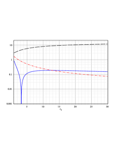
Figure 2: The combinations $\hat{\mu}/\mu$ (solid, blue), $\hat{m}/\mu$ (dot-dash, red) and $\hat{\lambda}\mu$ (dashed, black) as a function of $c_{2}$. $\hat{\mu}/\mu$ is negative for $c_{2}<\pi e^{2-\gamma}/\pi\approx 3.26$.

IV.3 Heuristic explanation

In both the nonrelativistic and massless cases the quadratic and quartic potential terms in the effective Lagrangian for the pair field have appropriate signs for the formation of a condensate. This is possible partly because the the four-fermion interaction is attractive, which gives the correct sign for the bare quadratic term, and partly because the nonthermal distribution generates conditions equivalent to the presence of a Fermi surface for high-momentum modes i.e. a nonnegligible chemical potential and low effective temperature. The latter is important both because it prevents the range of integration (which depends on the combination $\mu\beta$) used in deriving the coefficients from vanishing in the high temperature limit and because the transition temperature that enters the logarithm in the quadratic term is enhanced by a factor $\alpha$. Heuristically, this is a result of the fact that the interaction is not confined to a small region in momentum space as in the standard BCS case — i.e. it is a contact interaction — so the contribution of high-momentum modes is important.

It is also important to emphasise here that the torsion mediated interaction does not introduce a new coupling constant: the dependence of $\lambda_{0}$ on the Planck mass arises purely as a result of considering Einstein-Cartan gravity. The fermions themselves source the (non-propagating) torsion, as they have intrinsic spin.

The kinetic terms of the two examples differ: the massless fermion condensate has a purely propagating mode while the nonrelativistic case has a small, real, dissipative part. This would be dominant in the standard BCS case; here the asymmetry between the effective temperature felt by the modes on either side of the Fermi surface gives rise to an additional imaginary term. Although one also obtains a Gross-Pitaevski equation in the strong coupling limit of the BCS-BEC crossover, there these terms are absent because the chemical potential is negative, and the tightly-bound pairs cannot beak up. The difference arises in this model due to the inclusion of antifermions in the relativistic case, which cancel the real first order derivative terms entering the Lagrangian.

V Discussion

The starting action was (with the addition of the necessary curvature squared terms) renormalisable, however, in integrating out the antisymmetric part of the connection we have obtained an apparently nonrenormalisable four-fermion term. The status of this term seems a little different from the standard BCS case, in which the bare coupling constant $\lambda_{0}$ is renormalised by the considering the effective action for the fermions up to one-loop order. As this procedure could have been performed after renormalisation of the gravitational constant, $\lambda_{0}$ is already written in terms of renormalised quantities. As mentioned in the introduction, different approaches to this issue have been taken in the literature. A consistent approach would perhaps be to renormalise the entire Lagrangian (gravitational and fermion) simultaneously, although since the four-fermion interaction term is naively nonrenormalisable, it is not clear whether in this case $\lambda$ would simply be determined by the experimentally observed value. Here, despite the fact that integrating out $D_{\mu}{}^{I}{}_{J}$ can be done exactly, we have treated the resulting Lagrangian as an effective field theory valid up to a scale $\Lambda$, taken to be of the order of the scale defined by the inverse coupling $\lambda_{0}^{-1}\sim M_{\mathrm{pl}}$

This is important when treating the quadratic term in the effective Lagrangian for the pair field, since it is this term that represents a correction to the bare coupling. In the nonrelativistic calculation, the logarithmic dependence on the cutoff does not enter the effective Lagrangian explicitly, as the $\Lambda$ terms cancel when one expresses $\lambda_{0}^{-1}$ in terms of the binding energy $\epsilon_{a}$, calculated using the Schrödinger equation. In the relativistic calculation, since we have treated the fermions as massless fields, this is not possible. In Sec. IV.1.1, it is shown that there is in this case a linear dependence on $\Lambda/2\pi$, making it difficult to estimate the magnitude of this term. Consideration of the instantaneous Bethe-Salpeter equations for a spinless fermion-fermion bound state with a scalar interaction suggests that the combination that appears in this term, $\lambda_{0}^{-1}-\Lambda/2\pi$, should involve only negligible corrections of the order of the fermion mass. The form of the quadratic term $a|\Delta_{A}|^{2}$ is then logarithmic, as in the nonrelativistic case. For a rigorous treatment, one should include the mass from the beginning, however, since this introduces complications, we defer this to future work.

The equivalent calculation in the relativistic massive case would also be interesting because it would introduce another physical scale, the fermion mass, into the calculation. As mentioned in the introduction, many authors have focused on neutrino condensates with a view to relating the neutrino mass scale to dark energy. The condensation mechanism presented here is not particular to neutrinos, so one may think that if neutrinos can condense, so can other species. However, neutrinos are unusual in that they are the only known fundamental neutral fermions, so there is less competition between the gravitational interaction and gauge interactions compared to other species (cf. Barenboim:2010db ).

The result (90) takes the form of a Gross-Pitaevski theory describing a weakly interacting composite Bose gas. In the BCS-BEC crossover using nonrelativistic fermions, one finds a similar equation in the strong coupling regime Schakel:1999pa , where the bosons have twice the fermion mass. In this case, the mass of the boson is of the order of the only mass scale in the theory (with the exception of that defined by the coupling $\lambda_{0}^{-1}\sim M_{\mathrm{pl}}$) which is directly related to the inflaton mass. Thus, the mass of the boson in the effective field theory arises from the kinetic energy of the fermions. In the standard case, the appearance of a purely propagating mode in the BEC limit is related to the spontaneous breaking of the global U(1) symmetry i.e. $\Delta$ is a (pseudo) Goldstone mode. To fully understand and interpret the calculation presented here, it is therefore important to identify the role played by symmetry breaking. This is also particularly important in order to be able to comment on the change of vacuum energy of the system.

In our ansatz, thermalisation corresponds to the limit $\alpha\rightarrow 1$, at which point the fermions have a thermal distribution characterised by a high temperature $T=1/\beta$, such that $\beta\mu$ is negligible. It is important to note that one cannot take this limit directly in (90), since the assumptions (11) have been repeatedly used in the derivation. Since in this calculation $\mu$ is merely a scale used to parameterise the nonthermal distribution felt by the fermions subsequent to their creation in the preheating process, after thermalisation this should be replaced by a chemical potential term relating to any excess of fermions over antifermions, which should be zero.

Despite the fact that the inflaton field $\phi$ is also coupled to the fermions (perhaps indirectly) since the latter are produced by its decay, in this simplified description we have not included its effect directly. Although, like the four-fermion interaction (49), the Yukawa interaction $h\phi\bar{\psi}\psi$ is attractive, the effects of the two terms differ as $\phi$ acts like a mass term for the fermions, coupling $\bar{\psi}$ and $\psi$. To properly treat the thermalisation limit, one would need to include the effect of energy exchange between the fermions and the $\phi$-bosons; however, this is beyond the scope of this work.

To summarise, by considering a simplified model in 2+1 spacetime dimensions, we have shown for the first time that the nonthermal distribution of fermions arising from preheating after inflation can give rise to a fermion condensate. By considering the effective Lagrangian for the spacetime dependent pair field in the extreme cases of nonrelativistic and massless fermions, we have shown that it describes a gapless, propagating mode.

Appendix A Integrals and sums

The sums over the Matsubara frequencies are

$$\beta^{-1}\sum_{n}\frac{1}{\omega_{n}^{2}+\xi^{2}} = \frac{\tanh(\beta\xi/2)}{2\xi},$$ (94)

$$\beta^{-1}\sum_{n}\frac{1}{(\omega_{n}^{2}+\xi^{2})^{2}} = -\frac{1}{4\xi}\frac{d}{d\xi}\left(\frac{\tanh(\beta\xi/2)}{\xi}\right),$$ (95)

$$\beta^{-1}\sum_{n}\frac{1}{i\omega_{n}+\xi}\frac{1}{(i\omega_{n}-\xi)^{2}} = -\frac{1}{4}\frac{d}{d\xi}\left(\frac{\tanh(\beta\xi/2)}{\xi}\right),$$ (96)

$$\beta^{-1}\sum_{n}\frac{1}{i\omega_{n}+\xi}\frac{1}{(i\omega_{n}-\xi)^{3}} = -\frac{\tanh(\beta\xi/2)}{8\xi^{3}}-\frac{\beta}{16}\frac{d}{d\xi}\left(\frac{\mathrm{sech}^{2}(\beta\xi/2)}{\xi}\right).$$ (97)

We make use of the integral

$$\int_{0}^{a}\frac{X}{x}dx=\tanh(a)\ln(a)+\ln(4e^{\gamma}/\pi)+\int_{a}^{\infty}Y\ln(x)dx,$$ (98)

where $X\equiv\tanh(x)$ and $Y\equiv\mathrm{sech}^{2}(x)$ and $\gamma=0.577216\dots$ is the Euler-Mascheroni constant. Setting $a$ to 0 gives the result

$$\int_{0}^{\infty}Y\ln(x)dx=-\ln(4e^{\gamma}/\pi).$$ (99)

Also, the definite integral

$$\int_{0}^{\infty}\frac{XY}{x}dx=\frac{7}{\pi^{2}}\zeta(3),$$ (100)

can be combined with

$$\int_{0}^{a}\frac{dx}{x}\frac{d}{dx}\left(\frac{X}{x}\right)=\tfrac{1}{2}a^{-2}[\tanh(a)-a\ \mathrm{sech}^{2}(a)]-\int_{0}^{a}\frac{XY}{x}dx,$$ (101)

to give

$$\int_{0}^{\infty}\frac{dx}{x}\frac{d}{dx}\left(\frac{X}{x}\right)=-\frac{7}{\pi^{2}}\zeta(3).$$ (102)

Using this

$$\ \int_{0}^{\infty}x^{-3}[X-xY]dx=-\int_{0}^{\infty}\frac{dx}{x}\frac{d}{dx}\left(\frac{X}{x}\right)=\frac{7}{\pi^{2}}\zeta(3).$$ (103)

Principal value integrals with singularity and lower boundary occurring at $0$ can be treated with the formula Ramm:1990fk

$$\mathchoice{{\vbox{\hbox{$\textstyle=$ }}\kern-10.83342pt}}{{\vbox{\hbox{$\scriptstyle=$ }}\kern-7.76675pt}}{{\vbox{\hbox{$\scriptscriptstyle=$ }}\kern-6.08339pt}}{{\vbox{\hbox{$\scriptscriptstyle=$ }}\kern-5.58339pt}}\!\int_{0}^{a}\frac{f(x)}{x^{p+1}}dx=\int_{0}^{a}\frac{1}{x^{p+1}}\left[f(x)-\sum_{j=0}^{p}\frac{f^{(j)}(0)x^{j}}{j}\right]dx+\sum_{j=0}^{p-1}\frac{f^{(j)}(0)}{j!}\frac{a^{-p+j}}{j-p}+\frac{f^{(p)}(0)}{p!}\ln(a)$$ (104)

Taking $p=1$ and $p=2$ and $f(x)=X(x)$ gives

$$\mathchoice{{\vbox{\hbox{$\textstyle=$ }}\kern-10.83342pt}}{{\vbox{\hbox{$\scriptstyle=$ }}\kern-7.76675pt}}{{\vbox{\hbox{$\scriptscriptstyle=$ }}\kern-6.08339pt}}{{\vbox{\hbox{$\scriptscriptstyle=$ }}\kern-5.58339pt}}\!\int_{0}^{a}\frac{X}{x^{3}}dx =-\tfrac{1}{2}a^{-2}[\tanh(a)+a\ \mathrm{sech}^{2}(a)]-\int_{0}^{a}\frac{XY}{x}dx,$$ (105a)

$$\mathchoice{{\vbox{\hbox{$\textstyle=$ }}\kern-10.83342pt}}{{\vbox{\hbox{$\scriptstyle=$ }}\kern-7.76675pt}}{{\vbox{\hbox{$\scriptscriptstyle=$ }}\kern-6.08339pt}}{{\vbox{\hbox{$\scriptscriptstyle=$ }}\kern-5.58339pt}}\!\int_{0}^{a}\frac{X}{x^{2}}dx =1+\mathrm{sech}^{2}(a)\ln(a)-\frac{\tanh(a)}{a}+2\int_{0}^{a}XY\ln(x)dx.$$ (105b)

Using (105b) we obtain

$$\mathchoice{{\vbox{\hbox{$\textstyle=$ }}\kern-10.83342pt}}{{\vbox{\hbox{$\scriptstyle=$ }}\kern-7.76675pt}}{{\vbox{\hbox{$\scriptscriptstyle=$ }}\kern-6.08339pt}}{{\vbox{\hbox{$\scriptscriptstyle=$ }}\kern-5.58339pt}}\!\int_{0}^{\infty}\frac{X}{x^{2}}dx =1+2\int_{0}^{\infty}XY\ln(x)dx\equiv\eta,$$ (106a)

$$\mathchoice{{\vbox{\hbox{$\textstyle=$ }}\kern-10.83342pt}}{{\vbox{\hbox{$\scriptstyle=$ }}\kern-7.76675pt}}{{\vbox{\hbox{$\scriptscriptstyle=$ }}\kern-6.08339pt}}{{\vbox{\hbox{$\scriptscriptstyle=$ }}\kern-5.58339pt}}\!\int_{0}^{a}\frac{X}{x^{2}}dx \approx\ln(a),\qquad\qquad(a\ll 1)$$ (106b)

$$\mathchoice{{\vbox{\hbox{$\textstyle=$ }}\kern-10.83342pt}}{{\vbox{\hbox{$\scriptstyle=$ }}\kern-7.76675pt}}{{\vbox{\hbox{$\scriptscriptstyle=$ }}\kern-6.08339pt}}{{\vbox{\hbox{$\scriptscriptstyle=$ }}\kern-5.58339pt}}\!\int_{0}^{\infty}\frac{X}{x^{3}}dx =-\frac{7\zeta(3)}{\pi^{2}},$$ (106c)

$$\mathchoice{{\vbox{\hbox{$\textstyle=$ }}\kern-10.83342pt}}{{\vbox{\hbox{$\scriptstyle=$ }}\kern-7.76675pt}}{{\vbox{\hbox{$\scriptscriptstyle=$ }}\kern-6.08339pt}}{{\vbox{\hbox{$\scriptscriptstyle=$ }}\kern-5.58339pt}}\!\int_{0}^{a}\frac{X}{x^{2}}dx \approx-a^{-1}.\qquad\qquad(a\ll 1)$$ (106d)

Here, $\eta\approx 0.7905$ is a constant. For $a\gtrsim 1$ one can use the leading term of the asymptotic series approximation for the exponential integral, $E_{1}(z)=\frac{e^{-z}}{z}\sum_{n=0}^{N-1}\frac{n!}{(-z)^{n}}$, with $N=1$ to derive the following useful approximations

$$\int_{a}^{\infty}\frac{XY}{x}dx =-4\sum_{n=1}^{\infty}(-1)^{n}n^{2}E_{1}(2na)\simeq\frac{1}{2a}\mathrm{sech}^{2}(a), (a\gtrsim 1),$$ (107)

$$a\int_{a}^{\infty}\frac{X}{x^{2}}dx =1-2\sum_{n=1}^{\infty}(-1)^{n}\left[e^{-2na}+2naE_{1}(2na)\right]$$

$$\simeq 1+\frac{4}{1+e^{2a}}\approx 1. (a\gtrsim 1).$$ (108)

Appendix B Fierz identities

To derive the Fierz identities for the four-component representation, one can consider the basis:

$$\{I,\ \gamma^{\mu},\ \gamma^{35}\gamma^{\mu},\ \gamma^{3}\gamma^{\mu},\ \gamma^{5}\gamma^{\mu},\ i\gamma^{3},\ i\gamma^{5},\gamma^{35}\}.$$

However, the bilinears involving $\gamma^{3}$ and $\gamma^{5}$ do not transform simply under parity and charge conjugation, but instead transform as doublets. We have

$$\Phi=\begin{pmatrix}\bar{\psi}i\gamma^{3}\psi\\ \bar{\psi}i\gamma^{5}\psi\end{pmatrix},\qquad\Phi^{\mu}=\begin{pmatrix}\bar{\psi}\gamma^{3}\gamma^{\mu}\psi\\ \bar{\psi}\gamma^{5}\gamma^{\mu}\psi\end{pmatrix},$$ (109)

which are termed axi-scalar and axi-vector respectively in Burden:1991mb , as under parity they transform as $(\Phi)^{\mathcal{P}}=R_{P}\Phi$ and $(\Phi^{\mu})^{\mathcal{P}}=\Lambda^{\mu}{}_{\nu}R_{P}\Phi^{\mu}$ with $\Lambda^{\mu}{}_{\nu}=\mathrm{diag}(1,-1,1)$ and $R_{P}=\left(\begin{smallmatrix}-\cos(2\phi_{P})&\sin(2\phi_{P})\\ \sin(2\phi_{P})&\cos(2\phi_{P})\end{smallmatrix}\right)$. Introducing the shorthand

$$\begin{array}[]{lll}s_{1}=(\bar{\psi}_{4}\psi_{2})(\bar{\psi}_{3}\psi_{1})&&s_{2}=(\bar{\psi}_{4}\psi_{1})(\bar{\psi}_{3}\psi_{2})\\ v_{1}=(\bar{\psi}_{4}\gamma^{\mu}\psi_{2})(\bar{\psi}_{3}\gamma_{\mu}\psi_{1})&&v_{2}=(\bar{\psi}_{4}\gamma^{\mu}\psi_{1})(\bar{\psi}_{3}\gamma_{\mu}\psi_{2})\\ a_{1}=(\bar{\psi}_{4}\gamma^{35}\gamma^{\mu}\psi_{2})(\bar{\psi}_{3}\gamma^{35}\gamma_{\mu}\psi_{1})&&a_{2}=(\bar{\psi}_{4}\gamma^{35}\gamma^{\mu}\psi_{1})(\bar{\psi}_{3}\gamma^{35}\gamma_{\mu}\psi_{2})\\ x_{1}=(\Phi^{\dagger})_{(4;2)}(\Phi)_{(3;1)}&&x_{2}=(\Phi^{\dagger})_{(4;1)}(\Phi)_{(3;2)}\\ y_{1}=(\Phi^{\dagger}_{\mu})_{(4;2)}(\Phi^{\mu})_{(3;1)}&&y_{2}=(\Phi^{\dagger}_{\mu})_{(4;1)}(\Phi^{\mu})_{(3;2)}\\ z_{1}=(\bar{\psi}_{4}\gamma^{35}\psi_{2})(\bar{\psi}_{3}\gamma^{35}\psi_{1})&&z_{2}=(\bar{\psi}_{4}\gamma^{35}\psi_{1})(\bar{\psi}_{3}\gamma^{35}\psi_{2})\end{array}$$

where the subscripts on the $\Phi$ and $\Phi^{\mu}$ terms indicate the arrangement of the fermion bilinears that comprise the doublet, the Fierz identities are

$$\begin{pmatrix}s_{1}\\ v_{1}\\ a_{1}\\ x_{1}\\ y_{1}\\ z_{1}\end{pmatrix}=-\frac{1}{4}\begin{pmatrix}\hphantom{-}1&\hphantom{-}1&\hphantom{-}1&-1&-1&\hphantom{-}1\\ \hphantom{-}3&-1&-1&-1&\hphantom{-}3&\hphantom{-}3\\ \hphantom{-}3&-1&-1&\hphantom{-}1&-3&\hphantom{-}3\\ -6&-2&\hphantom{-}2&\hphantom{-}0&\hphantom{-}0&\hphantom{-}6\\ -2&\hphantom{-}2&-2&\hphantom{-}0&\hphantom{-}0&\hphantom{-}2\\ \hphantom{-}1&\hphantom{-}1&\hphantom{-}1&\hphantom{-}1&\hphantom{-}1&\hphantom{-}1\\ \end{pmatrix}\begin{pmatrix}s_{2}\\ v_{2}\\ a_{2}\\ x_{2}\\ y_{2}\\ z_{2}\end{pmatrix}.$$ (110)

When the four fermion fields are equal $\psi_{1}=\psi_{2}=\psi_{3}=\psi_{4}=\psi$, we can drop the subscripts on the variables $s_{1}$ to $z_{1}$ and obtain the relationship

$$3(s+z)+(a+v)=0.$$ (111)

Since the bilinears $s$ and $z$ are even under charge conjugation, and $v$ and $a$ are odd, we can conjugate one of the bilinears in each combination to get

$$3(s_{1}+z_{1})-(a_{1}+v_{1})=0,$$ (112)

where $\psi_{2}=\psi_{4}=\psi$ and $\psi_{3}=\psi_{1}=\psi^{c}$. Using (110) we find

$$v_{2}+a_{2}=0,$$ (113)

which can be substituted back into the identity for $z_{1}$ to give

$$m=m_{1}=-\tfrac{1}{4}[s_{2}+x_{2}+y_{2}+z_{2}].$$

More explicitly, this is

$$(\bar{\psi}\gamma^{35}\psi)^{2}=-\tfrac{1}{4}\left[(\bar{\psi}\psi^{c})(\bar{\psi}^{c}\psi)+(\bar{\psi}\gamma^{35}\psi^{c})(\bar{\psi}^{c}\gamma^{35}\psi)+\tilde{\Phi}^{\dagger}\tilde{\Phi}+\tilde{\Phi}^{\dagger}_{\mu}\tilde{\Phi}^{\mu}\right],$$ (114)

with

$$\tilde{\Phi}=\begin{pmatrix}\bar{\psi}^{c}i\gamma^{3}\psi\\ \bar{\psi}^{c}i\gamma^{5}\psi\end{pmatrix},\qquad\tilde{\Phi}^{\mu}=\begin{pmatrix}\bar{\psi}^{c}\gamma^{3}\gamma^{\mu}\psi\\ \bar{\psi}^{c}\gamma^{5}\gamma^{\mu}\psi\end{pmatrix}.$$ (115)

Appendix C Expansion terms

The quadratic part of the spatial Lagrangian can be expanded to second order in gradients as

$$\left[M_{Q_{1}}\nabla^{2}+M_{Q_{2}}(\vec{k}\cdot\vec{\nabla})^{2}-\frac{1}{\omega_{n}^{2}+\xi^{2}}-\frac{1}{\omega_{n}^{2}+\bar{\xi}^{2}}\right]|\Delta_{A}|^{2},$$

where

$$M_{Q_{1}} =-\frac{(\omega_{n}^{2}+\xi\bar{\xi})(2\omega_{n}^{2}+\xi^{2}+\bar{\xi}^{2})}{(\omega_{n}^{2}+\xi^{2})^{2}(\omega_{n}^{2}+\bar{\xi}^{2})^{2}},$$ (116a)

$$M_{Q_{2}} =\frac{4[(\omega_{n}^{2}+\xi\bar{\xi})^{2}-\omega^{2}_{n}(\xi-\bar{\xi})^{2}](2\omega_{n}^{2}+\xi^{2}+\bar{\xi}^{2})}{(\omega_{n}^{2}+\xi^{2})^{3}(\omega_{n}^{2}+\bar{\xi}^{2})^{3}}-\frac{4(\omega_{n}^{2}+\xi\bar{\xi})}{(\omega_{n}^{2}+\xi^{2})^{2}(\omega_{n}^{2}+\bar{\xi}^{2})^{2}}.$$ (116b)

The relevant Matsubara sums are

$$\beta^{-1}\sum_{n}M_{Q_{1}} =\frac{\beta}{8(\xi+\bar{\xi})}\left[\frac{\mathrm{sech}^{2}(\tfrac{1}{2}\beta\xi)}{\xi}+\frac{\mathrm{sech}^{2}(\tfrac{1}{2}\beta\bar{\xi})}{\bar{\xi}}\right]-$$

$$\quad-\frac{1}{4(\bar{\xi}-\xi)}\left[\frac{\tanh(\tfrac{1}{2}\beta\xi)}{\xi^{2}}-\frac{\tanh(\tfrac{1}{2}\beta\bar{\xi})}{\bar{\xi}^{2}}\right],$$ (117a)

$$\beta^{-1}\sum_{n}M_{Q_{2}} =-\frac{\beta^{2}}{4(\xi+\bar{\xi})^{2}}\left[\frac{\mathrm{sech}^{2}(\tfrac{1}{2}\beta\xi)\tanh(\tfrac{1}{2}\beta\xi)}{\xi}+\frac{\mathrm{sech}^{2}(\tfrac{1}{2}\beta\bar{\xi})\tanh(\tfrac{1}{2}\beta\bar{\xi})}{\bar{\xi}}\right]-$$

$$\quad-\frac{\beta}{4(\xi+\bar{\xi})^{3}}\left[\frac{\bar{\xi}+3\xi}{\xi^{2}}\mathrm{sech}^{2}(\tfrac{1}{2}\beta\xi)+\frac{3\bar{\xi}+\xi}{\bar{\xi}^{2}}\mathrm{sech}^{2}(\tfrac{1}{2}\beta\bar{\xi})\right]+$$

$$\quad+\frac{1}{2(\bar{\xi}^{2}-\xi^{2})}\left[\frac{\tanh(\tfrac{1}{2}\beta\xi)}{\xi^{3}}-\frac{\tanh(\tfrac{1}{2}\beta\bar{\xi})}{\bar{\xi}^{3}}\right].$$ (117b)

Appendix D The time-dependent Lagrangian to second order

D.1 Nonrelativistic case

Using (106), the terms second order in $q_{0}$ in (23) are

$$\begin{split}Q^{\prime}(q_{0})&\supset\frac{\nu(0)}{2}\frac{\alpha^{2}\beta^{2}q_{0}^{2}}{16}\left[\frac{1}{\alpha^{4}}\mathchoice{{\vbox{\hbox{$\textstyle=$ }}\kern-10.83342pt}}{{\vbox{\hbox{$\scriptstyle=$ }}\kern-7.76675pt}}{{\vbox{\hbox{$\scriptscriptstyle=$ }}\kern-6.08339pt}}{{\vbox{\hbox{$\scriptscriptstyle=$ }}\kern-5.58339pt}}\!\int_{-c_{1}}^{0}\frac{X}{x^{3}}dx+\mathchoice{{\vbox{\hbox{$\textstyle=$ }}\kern-10.83342pt}}{{\vbox{\hbox{$\scriptstyle=$ }}\kern-7.76675pt}}{{\vbox{\hbox{$\scriptscriptstyle=$ }}\kern-6.08339pt}}{{\vbox{\hbox{$\scriptscriptstyle=$ }}\kern-5.58339pt}}\!\int_{0}^{\infty}\frac{X}{x^{3}}dx\right],\\ &\simeq-\frac{\nu(0)}{2}\frac{\alpha^{2}\beta^{2}q_{0}^{2}}{16}\left[\frac{7\zeta(3)}{\pi^{2}}+\frac{1}{\alpha^{4}c_{1}}\right],\\ &\simeq-\frac{\nu(0)}{2}\frac{\alpha^{2}\beta^{2}q_{0}^{2}}{16},\end{split}$$ (118)

where in the third line, we have neglected the subdominant term $1/(\alpha^{4}c_{1})=1/(\alpha^{2}c_{2})\ll 1$ as $\alpha$ is large. After integrating by parts, the dynamical part of the Lagrangian to second order is

$$\mathcal{L}^{(2)}_{\rm dyn}\simeq\left(\frac{m}{2\pi}\right)\frac{7\alpha^{2}\beta^{2}\zeta(3)}{32\pi^{2}}\Delta^{*}\partial_{0}^{2}\Delta.$$ (119)

D.2 Relativistic case

If we were to expand up to second order in $q_{0}$ in (85) the integration by parts gives a relative plus sign. The $q_{0}^{2}$ terms cancel exactly and we have only to evaluate the hypersingular integral $Q_{\xi}^{\prime}(q_{0})$ and the integral $Q_{\bar{\xi}}^{\prime}(q_{0})$, given by

$$\begin{split}Q_{\xi}^{\prime}(q_{0})&=\frac{q_{0}^{2}\alpha\beta}{32\pi}\left\{\frac{1}{\alpha^{2}}\mathchoice{{\vbox{\hbox{$\textstyle=$ }}\kern-10.83342pt}}{{\vbox{\hbox{$\scriptstyle=$ }}\kern-7.76675pt}}{{\vbox{\hbox{$\scriptscriptstyle=$ }}\kern-6.08339pt}}{{\vbox{\hbox{$\scriptscriptstyle=$ }}\kern-5.58339pt}}\!\int_{-c_{1}}^{0}dx\frac{(x+c_{1})X}{x^{3}}+\mathchoice{{\vbox{\hbox{$\textstyle=$ }}\kern-10.83342pt}}{{\vbox{\hbox{$\scriptstyle=$ }}\kern-7.76675pt}}{{\vbox{\hbox{$\scriptscriptstyle=$ }}\kern-6.08339pt}}{{\vbox{\hbox{$\scriptscriptstyle=$ }}\kern-5.58339pt}}\!\int_{0}^{\infty}dx\frac{(x+c_{2})X}{x^{3}}\right\},\\ &\simeq-\frac{q_{0}^{2}\alpha\beta}{32\pi}\left\{\frac{1}{\alpha^{2}}[1+\ln(c_{1})]-\eta+\frac{7\zeta(3)}{\pi^{2}}c_{2}\right\},\end{split}$$ (120)

where in the second line we have evaluated the principal value integrals using (105), keeping only the non-vanishing terms as $c_{1}\rightarrow 0$, and

$$\begin{split}Q_{\bar{\xi}}^{\prime}(q_{0})&=\frac{q_{0}^{2}\alpha\beta}{32\pi}\left\{\frac{1}{\alpha^{2}}\mathchoice{{\vbox{\hbox{$\textstyle=$ }}\kern-10.83342pt}}{{\vbox{\hbox{$\scriptstyle=$ }}\kern-7.76675pt}}{{\vbox{\hbox{$\scriptscriptstyle=$ }}\kern-6.08339pt}}{{\vbox{\hbox{$\scriptscriptstyle=$ }}\kern-5.58339pt}}\!\int_{c_{1}}^{2c_{1}}dx\frac{(x-c_{1})X}{x^{3}}+\mathchoice{{\vbox{\hbox{$\textstyle=$ }}\kern-10.83342pt}}{{\vbox{\hbox{$\scriptstyle=$ }}\kern-7.76675pt}}{{\vbox{\hbox{$\scriptscriptstyle=$ }}\kern-6.08339pt}}{{\vbox{\hbox{$\scriptscriptstyle=$ }}\kern-5.58339pt}}\!\int_{2c_{2}}^{\infty}dx\frac{(x-c_{2})X}{x^{3}}\right\},\\ &\simeq\frac{q_{0}^{2}\alpha\beta}{32\pi}\left\{\frac{1}{\alpha^{2}}\left[\ln 2-\frac{1}{2}\right]+\frac{3}{8c_{2}}\tanh(2c_{2})-\mathrm{sech}^{2}(2c_{2})\ln(2c_{2})+2\int_{2c_{2}}^{\infty}XY\ln(x)dx\right\},\\ &\lesssim\frac{q_{0}^{2}\alpha\beta}{32\pi}\left\{\frac{1}{\alpha^{2}}\left[\ln 2-\frac{1}{2}\right]+\frac{1}{2}\right\}.\end{split}$$ (121)

This is valid for $c_{2}\gtrsim 1$ as in the second line we have integrated by parts and used (107), and in the third line noted that the expression is a decreasing function of $c_{2}$. Combining (120) and (121), we have

$$Q_{\xi}^{\prime}(q_{0})+Q_{\bar{\xi}}^{\prime}(q_{0})\approx-\frac{q_{0}^{2}\alpha\beta}{32\pi}\left(\frac{\ln(c_{1})}{\alpha^{2}}+\frac{7\zeta(3)}{\pi^{2}}c_{2}\right)\approx-\frac{q_{0}^{2}\alpha\beta}{32\pi}\frac{7\zeta(3)}{\pi^{2}}c_{2},$$ (122)

modulo corrections by subdominant numerical factors $\sim\mathcal{O}(1)$ inside the parentheses. In the second approximation, we have used the fact that for large $\alpha$ we have

$$\frac{\ln(c_{1})}{\alpha^{2}}+\frac{7\zeta(3)}{\pi^{2}}c_{2}=\frac{\ln(c_{2}/\alpha^{2})}{\alpha^{2}}+\frac{7\zeta(3)}{\pi^{2}}c_{2}\rightarrow\frac{7\zeta(3)}{\pi^{2}}c_{2},$$

so the second term is dominant. The correction to the Lagrangian (86) is then

$$\mathcal{L}_{\rm dyn}^{(2)}\approx\left(\frac{\mu}{2\pi}\right)\frac{7\alpha^{2}\beta^{2}\zeta(3)}{32\pi^{2}}\Delta_{A}^{\dagger}\partial_{0}^{2}\Delta_{A}.$$ (123)

Comparing with (119) it can be seen that the scale $\mu$ enters in the same way as the mass of the fermions in the nonrelativistic case. In the nonrelativistic case, the $\mathcal{L}_{\rm dyn}^{(2)}$ represents the second term in series expansion in $q_{0}/T$, which appears in the Lagrangian as the Cooper pairs can break up. The presence of an equivalent term in the relativistic case suggests that the weakly interacting bosons described by (90) are not stable, although this is most important for the higher energy modes.

References

- (1) L. Parker and D. Toms, Quantum field theory in curved spacetime. Quantized fields and gravity. (Cambridge Monographs on Mathematical Physics. Cambridge University Press, 2009).
- (2) C. W. Misner, K. S. Thorne, J. A. Wheeler, Gravitation (Freeman, San Francisco, 1973).
- (3) T. Kibble, J.Math.Phys. 2, 212 (1961).
- (4) G. de Berredo-Peixoto, L. Freidel, I. Shapiro, and C. de Souza, JCAP 1206, 017 (2012), 1201.5423.
- (5) J. Magueijo, T. Zlosnik, and T. Kibble, Phys.Rev.D 87, 063504 (2013), 1212.0585.
- (6) B. P. Dolan, Class.Quant.Grav. 27, 095010 (2010), 0911.1636.
- (7) I. Khriplovich and A. Rudenko, JCAP 1211, 040 (2012), 1210.7306.
- (8) I. Khriplovich and A. Rudenko, (2013), 1303.1348.
- (9) N. J. Poplawski, Annalen Phys. 523, 291 (2011), 1005.0893.
- (10) N. J. Poplawski, Gen.Rel.Grav. 44, 491 (2012), 1102.5667.
- (11) D. R. Brill and J. A. Wheeler, Rev.Mod.Phys. 29, 465 (1957).
- (12) D. Caldi and A. Chodos, (1999), hep-ph/9903416.
- (13) M. Blasone, A. Capolupo, S. Capozziello, S. Carloni, and G. Vitiello, Phys.Lett. A323, 182 (2004), gr-qc/0402013.
- (14) G. Barenboim, Phys.Rev. D82, 093014 (2010), 1009.2504.
- (15) S. Alexander, T. Biswas, and G. Calcagni, Phys.Rev. D81, 043511 (2010), 0906.5161.
- (16) S. Alexander, T. Biswas, and G. Calcagni, Phys. Rev. D 81, 069902(E) (2010).
- (17) S. Alexander and T. Biswas, Phys.Rev. D80, 023501 (2009), 0807.4468.
- (18) S. H. Alexander and D. Vaid, (2006), hep-th/0609066.
- (19) P. D. Serpico and G. G. Raffelt, Phys.Rev. D71, 127301 (2005), astro-ph/0506162.
- (20) L. Kofman, A. D. Linde, and A. A. Starobinsky, Phys.Rev. D56, 3258 (1997), hep-ph/9704452.
- (21) P. B. Greene and L. Kofman, Phys.Rev. D62, 123516 (2000), hep-ph/0003018.
- (22) J. Berges, S. Borsanyi, and C. Wetterich, Phys.Rev.Lett. 93, 142002 (2004), hep-ph/0403234.
- (23) J. Berges, D. Gelfand, and J. Pruschke, Phys.Rev.Lett. 107, 061301 (2011), arXiv: 1012.4632.
- (24) S. Deser, R. Jackiw, and G. ’t Hooft, Annals Phys. 152, 220 (1984).
- (25) S. Carlip, Class.Quant.Grav. 22, R85 (2005), gr-qc/0503022.
- (26) M. Hortacsu, H. Ozcelik, and N. Ozdemir, (2008), 0807.4413.
- (27) T. Dereli, N. Özdemir, and Ö. Sert, Eur.Phys.J. C73, 2279 (2013), 1002.0958.
- (28) A. M. Schakel, Time dependent Ginzburg-Landau theory and duality, in Topological defects and the nonequilibrium dynamics of symmetry breaking phase transitions: proceedings, edited by Y. M. Bunkov and H. Godrin, , NATO Science Series C: Mathematical and Physical Science Vol. 549, pp. 213–238, 2000, arXiv:cond-mat/9904092.
- (29) J. Chluba and R. A. Sunyaev, Monthly Notices of the Royal Astronomical Society 419, 1294 (2012).
- (30) C. Sa de Melo, M. Randeria, and J. R. Engelbrecht, Phys.Rev.Lett. 71, 3202 (1993).
- (31) M. de Jesus Anguiano Galicia and A. Bashir, Few Body Syst. 37, 71 (2005), hep-ph/0502089.
- (32) K. Shimizu, Prog.Theor.Phys. 74, 610 (1985).
- (33) J. Deng, A. Schmitt, and Q. Wang, Phys.Rev. D76, 034013 (2007), nucl-th/0611097.
- (34) C. Burden, Nucl.Phys. B387, 419 (1992).
- (35) N. Dadhich and J. M. Pons, Gen.Rel.Grav. 44, 2337 (2012), 1010.0869.
- (36) T. Ohsaku, International Journal of Modern Physics B 18, 1771 (2004).
- (37) Y. Nishida and H. Abuki, Phys.Rev. D72, 096004 (2005), hep-ph/0504083.
- (38) L. He and P. Zhuang, Phys.Rev. D75, 096003 (2007), hep-ph/0703042.
- (39) L. Suttorp, Annals Phys. 122, 397 (1979).
- (40) E. Abrahams and T. Tsuneto, Phys.Rev. 152, 416 (1966).
- (41) J. O. Andersen, Rev.Mod.Phys. 76, 599 (2004), cond-mat/0305138.
- (42) M. Drechsler and W. Zwerger, Annalen der Physik 504, 15 (1992).
- (43) A. Ramm and A. Sluis, Numerische Mathematik 57, 139 (1990).