Abstract

In this article, we study momentum dependence of the hadronic coupling constants $G_{B_{c}^{*}B_{c}\Upsilon}$, $G_{B_{c}^{*}B_{c}J/\psi}$, $G_{B_{c}B_{c}\Upsilon}$ and $G_{B_{c}B_{c}J/\psi}$ with the off-shell $\Upsilon$ and $J/\psi$ using the three-point QCD sum rules. Then we fit the hadronic coupling constants into analytical functions and extrapolate them into deep time-like regions to obtain the on-shell values $G_{B_{c}^{*}B_{c}\Upsilon}(q^{2}=M_{\Upsilon}^{2})$, $G_{B_{c}^{*}B_{c}J/\psi}(q^{2}=M_{J/\psi}^{2})$, $G_{B_{c}B_{c}\Upsilon}(q^{2}=M_{\Upsilon}^{2})$ and $G_{B_{c}B_{c}J/\psi}(q^{2}=M_{J/\psi}^{2})$ for the first time. Those hadronic coupling constants can be taken as basic input parameters in phenomenological analysis.

PACS number: 12.38.Lg, 14.40.Pq

Key words: QCD sum rules, Heavy quarkonium

1 Introduction

The suppression of $J/\psi$ production in relativistic heavy ion collisions is considered as an important signature to identify the quark-gluon plasma [1]. The dissociation of $J/\psi$ in the quark-gluon plasma due to color screening can lead to a reduction of its production. The bottomonium states are also sensitive to the color screening, the $\Upsilon$ suppression in high energy heavy ion collisions can also be taken as a signature to identify the quark-gluon plasma [2]. The suppressions on the $\Upsilon$ production in ultra-relativistic heavy ion collisions will be studied in details at the Relativistic Heavy Ion Collider (RHIC) and Large Hadron Collider (LHC). Before drawing a definite conclusion on appearance of the quark-gluon plasma, we have to disentangle the color screening versus recombination of the off-diagonal $\bar{c}c$ (or $\bar{b}b$ ) pairs in the hot dense medium versus cold nuclear matter effects such as nuclear absorption, shadowing and anti-shadowing [3, 4].

We can study the heavy quarkonium absorptions with the effective Lagrangians in meson-exchange models [5], and calculate the absorption cross sections based on the interactions among the heavy quarkonia and heavy mesons, where the hadronic coupling constants are basic input parameters. The detailed knowledge of the hadronic coupling constants is of great importance in understanding the effects of heavy quarkonium absorptions in hadronic matter. Furthermore, the hadronic coupling constants among the heavy quarkonia and heavy mesons play an important role in understanding final-state interactions in the heavy quarkonium decays [6].

The hadronic coupling constants in the $D^{*}D\pi$, $D^{*}D_{s}K$, $D_{s}^{*}DK$, $B^{*}B\pi$, $B^{*}_{s}BK$, $DD\rho$, $D_{s}DK^{*}$, $B_{s}BK^{*}$, $D^{*}D\rho$, $D^{*}_{s}DK^{*}$, $B^{*}_{s}BK^{*}$, $D^{*}D^{*}\rho$, $B^{*}B^{*}\rho$, $B_{s0}BK$, $B_{s1}B^{*}K$, $D^{*}_{s}DK_{1}$, $B^{*}_{s}BK_{1}$, $J/\psi DD$, $J/\psi DD^{*}$, $J/\psi D^{*}D^{*}$ vertices have been studied with the three-point QCD sum rules (QCDSR) [7, 8], while the hadronic coupling constants in the $D^{*}D\pi$, $D^{*}D_{s}K$, $D^{*}_{s}DK$, $B^{*}B\pi$, $DD\rho$, $DD_{s}K^{*}$, $D_{s}D_{s}\phi$, $BB\rho$, $D^{*}D\rho$, $D^{*}D_{s}K^{*}$, $D_{s}^{*}D_{s}\phi$, $B^{*}B\rho$, $D^{*}D^{*}\pi$, $D^{*}D_{s}^{*}K$, $B^{*}B^{*}\pi$, $D^{*}D^{*}\rho$, $D_{0}D\pi$, $B_{0}B\pi$, $D_{0}D_{s}K$, $D_{s0}DK$, $B_{s0}BK$, $D_{1}D^{*}\pi$, $B_{1}B^{*}\pi$, $D_{s1}D^{*}K$, $B_{s1}B^{*}K$, $B_{1}B_{0}\pi$, $B_{2}B_{1}\pi$, $B_{2}B^{*}\pi$, $B_{1}B^{*}\rho$, $B_{1}B\rho$, $B_{2}B^{*}\rho$, $B_{2}B_{1}\rho$ vertices have been studied with the light-cone QCDSR [9].

To my knowledge, the hadronic coupling constants among the heavy quarkonium states have not been studied with the three-point QCDSR or light-cone QCDSR. In the article, we study the vertices $B_{c}^{*}B_{c}\Upsilon$, $B_{c}^{*}B_{c}J/\psi$, $B_{c}B_{c}\Upsilon$ and $B_{c}B_{c}J/\psi$ with the three-point QCDSR. The QCD sum rules is a powerful nonperturbative approach in studying the heavy quarkonium states, and has given many successful descriptions of the masses, decay constants, form-factors, hadronic coupling constants [10, 11, 12].

The $B_{c}^{*\pm}$ mesons have not been observed yet, but they are expected to be observed at the LHC through the radiative transitions. In previous works, we study the vector and axial-vector $B_{c}$ mesons with the QCDSR, make reasonable predictions of the masses and decay constants, then calculate the $B_{c}^{*}\to B_{c}$ electromagnetic form-factor with the three-point QCDSR, and obtain the decay width of the radiative transitions $B_{c}^{*\pm}\to B_{c}^{\pm}\gamma$ [13, 14].

The article is arranged as follows: we study the $B_{c}^{*}B_{c}\Upsilon$, $B_{c}^{*}B_{c}J/\psi$, $B_{c}B_{c}\Upsilon$ and $B_{c}B_{c}J/\psi$ vertices using the three-point QCDSR in Sect.2; in Sect.3, we present the numerical results and discussions; and Sect.4 is reserved for our conclusions.

2 The $B_{c}^{*}B_{c}\Upsilon$ and $B_{c}B_{c}\Upsilon$ (also $B_{c}^{*}B_{c}J/\psi$ and $B_{c}B_{c}J/\psi$) vertices with QCD sum rules

We study the $B_{c}^{*}B_{c}\Upsilon$ and $B_{c}B_{c}\Upsilon$ vertices with the three-point correlation functions $\Pi_{\mu\nu}(p,p^{\prime})$ and $\Pi_{\mu}(p,p^{\prime})$, respectively,

$$\Pi_{\mu\nu}(p,p^{\prime}) = i^{2}\int d^{4}xd^{4}ye^{ip^{\prime}\cdot x+i(p-p^{\prime})\cdot y}\langle 0|T\left\{J_{5}(x)j_{\mu}(y)J_{\nu}^{\dagger}(0)\right\}|0\rangle\,,$$

$$\Pi_{\mu}(p,p^{\prime}) = i^{2}\int d^{4}xd^{4}ye^{ip^{\prime}\cdot x+i(p-p^{\prime})\cdot y}\langle 0|T\left\{J_{5}(x)j_{\mu}(y)J_{5}^{\dagger}(0)\right\}|0\rangle\,,$$ (1)

where

$$j_{\mu}(x) = \bar{b}(x)\gamma_{\mu}b(x)\,,$$

$$J_{5}(x) = \bar{c}(x)i\gamma_{5}b(x)\,,$$

$$J^{\dagger}_{\nu}(x) = \bar{b}(x)\gamma_{\nu}c(x)\,,$$ (2)

the currents $j_{\mu}(x)$, $J_{5}(x)$ and $J^{\dagger}_{\nu}(x)$ interpolate the heavy quarkonia $\Upsilon$, $B_{c}$ and $B_{c}^{*}$, respectively.

We can insert a complete set of intermediate hadronic states with the same quantum numbers as the current operators $j_{\mu}(y)$, $J_{5}(x)$, $J^{\dagger}_{\nu}(0)$ and $J^{\dagger}_{5}(0)$ into the correlation functions $\Pi_{\mu\nu}(p,p^{\prime})$ and $\Pi_{\mu}(p,p^{\prime})$ to obtain the hadronic representation [10, 11]. After isolating the ground state contributions come from the heavy quarkonia $\Upsilon$, $B_{c}$ and $B_{c}^{*}$, we get the following results,

$$\Pi_{\mu\nu}(p,p^{\prime}) = \frac{\langle 0|J_{5}(0)|B_{c}(p^{\prime})\rangle\langle 0|j_{\mu}(0)|\Upsilon(q)\rangle\langle B_{c}^{*}(p)|J^{\dagger}_{\nu}(0)|0\rangle\langle B_{c}(p^{\prime})\Upsilon(q)|{\mathcal{L}}(0)|B_{c}^{*}(p)\rangle}{(M_{B_{c}}^{2}-p^{\prime 2})(M_{\Upsilon}^{2}-q^{2})(M_{B_{c}^{*}}^{2}-p^{2})}+\cdots\,,$$ (3)

$$= -\frac{f_{B_{c}}M_{B_{c}}^{2}f_{B_{c}^{*}}M_{B_{c}^{*}}f_{\Upsilon}M_{\Upsilon}}{(m_{b}+m_{c})(M_{B_{c}}^{2}-p^{\prime 2})(M_{B_{c}^{*}}^{2}-p^{2})(M_{\Upsilon}^{2}-q^{2})}\,G_{B_{c}^{*}B_{c}\Upsilon}(q^{2})\,\epsilon_{\mu\nu\alpha\beta}p^{\alpha}p^{\prime\beta}+\cdots\,,$$

$$\Pi_{\mu}(p,p^{\prime}) = \frac{\langle 0|J_{5}(0)|B_{c}(p^{\prime})\rangle\langle 0|j_{\mu}(0)|\Upsilon(q)\rangle\langle B_{c}(p)|J^{\dagger}_{5}(0)|0\rangle\langle B_{c}(p^{\prime})\Upsilon(q)|{\mathcal{L}}(0)|B_{c}(p)\rangle}{(M_{B_{c}}^{2}-p^{\prime 2})(M_{\Upsilon}^{2}-q^{2})(M_{B_{c}}^{2}-p^{2})}+\cdots\,,$$ (4)

$$= \frac{f_{B_{c}}^{2}M_{B_{c}}^{4}f_{\Upsilon}M_{\Upsilon}}{(m_{b}+m_{c})^{2}(M_{B_{c}}^{2}-p^{\prime 2})(M_{B_{c}}^{2}-p^{2})(M_{\Upsilon}^{2}-q^{2})}\,G_{B_{c}B_{c}\Upsilon}(q^{2})\,(p+p^{\prime})_{\mu}+\cdots\,,$$

$$= \Gamma_{p}(p,p^{\prime})p_{\mu}+\Gamma_{p^{\prime}}(p,p^{\prime})p^{\prime}_{\mu}+\cdots\,,$$

where we have used the following effective Lagrangian ${\mathcal{L}}$ and definitions for the decay constants $f_{B_{c}^{*}}$, $f_{B_{c}}$, $f_{\Upsilon}$,

$${\mathcal{L}} = G_{B_{c}^{*}B_{c}\Upsilon}\,\epsilon_{\lambda\tau\rho\sigma}B_{c}^{\dagger}\partial^{\lambda}\Upsilon^{\tau}\partial^{\rho}B_{c}^{*\sigma}+iG_{B_{c}B_{c}J/\psi}\Upsilon^{\mu}\left(B_{c}^{\dagger}\partial_{\mu}B_{c}-\partial_{\mu}B_{c}^{\dagger}B_{c}\right)\,,$$ (5)

$$\langle 0|J_{\mu}(0)|B_{c}^{*}(p)\rangle = f_{B_{c}^{*}}M_{B_{c}^{*}}\zeta_{\mu}\,,$$

$$\langle 0|J_{5}(0)|B_{c}(p^{\prime})\rangle = \frac{f_{B_{c}}M_{B_{c}}^{2}}{m_{b}+m_{c}}\,,$$

$$\langle 0|j_{\mu}(0)|\Upsilon(q)\rangle = f_{\Upsilon}M_{\Upsilon}\xi_{\mu}\,,$$ (6)

$q_{\mu}=(p-p^{\prime})_{\mu}$, the $\zeta_{\mu}$ and $\xi_{\mu}$ are the polarization vectors. The tensor structures $p_{\mu}$ and $p^{\prime}_{\mu}$ associate with the correlation functions $\Gamma_{p}(p,p^{\prime})$ and $\Gamma_{p^{\prime}}(p,p^{\prime})$, respectively, we obtain the QCDSR by considering the combination $\Gamma_{p}(p,p^{\prime})+\Gamma_{p^{\prime}}(p,p^{\prime})$.

The effective fields describe point-like particles only in the case that all the interacting particles are on the mass-shell. When at least one particle in the vertex is off-shell, the finite-size effects of the hadrons become important. We should introduce form-factors in the hadronic coupling constants to parameterize the off-shell effects, which are of great importance in calculating scattering amplitudes at the hadronic level. In this article, we parameterize the $q^{2}$ dependence of the hadronic coupling constants $G(q^{2})$ with suitable functions, then obtain the on-shell values $G(q^{2}=-Q^{2}=M_{\Upsilon}^{2})$ by analytically continuing the $q^{2}$ to the physical region.

Now, we briefly outline the operator product expansion for the correlation functions $\Pi_{\mu\nu}(p,p^{\prime})$ and $\Pi_{\mu}(p,p^{\prime})$. We contract the quark fields in the correlation functions $\Pi_{\mu\nu}(p,p^{\prime})$ and $\Pi_{\mu}(p,p^{\prime})$ with Wick theorem firstly,

$$\Pi_{\mu\nu}(p,p^{\prime}) = \int d^{4}xd^{4}ye^{ip^{\prime}\cdot x+i(p-p^{\prime})\cdot y}\,\,{\rm Tr}\left\{i\gamma_{5}B^{mn}(x-y)\gamma_{\mu}B^{nk}(y)\gamma_{\nu}C^{km}(-x)\right\}\,,$$

$$\Pi_{\mu}(p,p^{\prime}) = \int d^{4}xd^{4}ye^{ip^{\prime}\cdot x+i(p-p^{\prime})\cdot y}\,\,{\rm Tr}\left\{i\gamma_{5}B^{mn}(x-y)\gamma_{\mu}B^{nk}(y)i\gamma_{5}C^{km}(-x)\right\}\,,$$ (7)

replace the $b$ and $c$ quark propagators $B^{ij}(x)$ and $C^{ij}(x)$ with the corresponding full propagators $S_{ij}(x)$,

$$S_{ij}(x) = \frac{i}{(2\pi)^{4}}\int d^{4}ke^{-ik\cdot x}\left\{\frac{\delta_{ij}}{\!\not\!{k}-m_{Q}}-\frac{g_{s}G^{n}_{\alpha\beta}t^{n}_{ij}}{4}\frac{\sigma^{\alpha\beta}(\!\not\!{k}+m_{Q})+(\!\not\!{k}+m_{Q})\sigma^{\alpha\beta}}{(k^{2}-m_{Q}^{2})^{2}}+\frac{\delta_{ij}\langle g^{2}_{s}GG\rangle}{12}\right.$$ (8)

$$\left.\frac{m_{Q}k^{2}+m_{Q}^{2}\!\not\!{k}}{(k^{2}-m_{Q}^{2})^{4}}+\cdots\right\}\,,$$

where $Q=c,b$, $\langle g^{2}_{s}GG\rangle=\langle g^{2}_{s}G^{n}_{\alpha\beta}G^{n\alpha\beta}\rangle$, $t^{n}=\frac{\lambda^{n}}{2}$, the $\lambda^{n}$ are the Gell-Mann matrixes, the $i$, $j$ are color indexes [11], then compute the integrals. In this article, we take into account the leading-order contributions $\Pi_{\mu\nu}^{0}(p,p^{\prime})$, $\Pi_{\mu}^{0}(p,p^{\prime})$ and gluon condensate contributions $\Pi_{\mu\nu}^{GG}(p,p^{\prime})$, $\Pi_{\mu}^{GG}(p,p^{\prime})$ in the operator product expansion, and show them explicitly using the Feynman diagrams in Figs.1-2.

The leading-order contributions $\Pi_{\mu\nu}^{0}(p,p^{\prime})$, $\Pi_{\mu}^{0}(p,p^{\prime})$ can be written as

$$\Pi_{\mu\nu}^{0}(p,p^{\prime}) = \frac{3}{(2\pi)^{4}}\int d^{4}k\frac{{\rm Tr}\left\{\gamma_{5}\left[\!\not\!{k}+m_{b}\right]\gamma_{\mu}\left[\!\not\!{k}+\!\not\!{p}-\!\not\!{p^{\prime}}+m_{b}\right]\gamma_{\nu}\left[\!\not\!{k}-\!\not\!{p^{\prime}}+m_{c}\right]\right\}}{\left[k^{2}-m_{b}^{2}\right]\left[(k+p-p^{\prime})^{2}-m_{b}^{2}\right]\left[(k-p^{\prime})^{2}-m_{c}^{2}\right]}\,,$$ (9)

$$= \int dsdu\frac{\rho_{\mu\nu}(s,u,q^{2})}{(s-p^{2})(u-p^{\prime 2})}\,,$$

$$\Pi_{\mu}^{0}(p,p^{\prime}) = \frac{3i}{(2\pi)^{4}}\int d^{4}k\frac{{\rm Tr}\left\{\gamma_{5}\left[\!\not\!{k}+m_{b}\right]\gamma_{\mu}\left[\!\not\!{k}+\!\not\!{p}-\!\not\!{p^{\prime}}+m_{b}\right]\gamma_{5}\left[\!\not\!{k}-\!\not\!{p^{\prime}}+m_{c}\right]\right\}}{\left[k^{2}-m_{b}^{2}\right]\left[(k+p-p^{\prime})^{2}-m_{b}^{2}\right]\left[(k-p^{\prime})^{2}-m_{c}^{2}\right]}\,,$$ (10)

$$= \int dsdu\frac{\rho_{\mu}(s,u,q^{2})}{(s-p^{2})(u-p^{\prime 2})}\,.$$

We put all the quark lines on mass-shell using the Cutkosky’s rules, see Fig.1, and obtain the leading-order spectral densities $\rho_{\mu\nu}(s,u,q^{2})$ and $\rho_{\mu}(s,u,q^{2})$,

$$\rho_{\mu\nu}(s,u,q^{2}) = -\frac{3i}{(2\pi)^{3}}\int d^{4}k\delta\left[k^{2}-m_{b}^{2}\right]\delta\left[(k+p-p^{\prime})^{2}-m_{b}^{2}\right]\delta\left[(k-p^{\prime})^{2}-m_{c}^{2}\right]$$ (11)

$${\rm Tr}\left\{\gamma_{5}\left[\!\not\!{k}+m_{b}\right]\gamma_{\mu}\left[\!\not\!{k}+\!\not\!{p}-\!\not\!{p^{\prime}}+m_{b}\right]\gamma_{\nu}\left[\!\not\!{k}-\!\not\!{p^{\prime}}+m_{c}\right]\right\}$$

$$= -\frac{3\epsilon_{\mu\nu\alpha\beta}p^{\alpha}p^{\prime\beta}}{4\pi^{2}\sqrt{\lambda(s,u,q^{2})}}\left\{m_{b}+\frac{(m_{b}-m_{c})(s+u-q^{2}+2m_{b}^{2}-2m_{c}^{2})q^{2}}{\lambda(s,u,q^{2})}\right\}\,,$$

$$\rho_{\mu}(s,u,q^{2}) = \frac{3}{(2\pi)^{3}}\int d^{4}k\delta\left[k^{2}-m_{b}^{2}\right]\delta\left[(k+p-p^{\prime})^{2}-m_{b}^{2}\right]\delta\left[(k-p^{\prime})^{2}-m_{c}^{2}\right]$$ (12)

$${\rm Tr}\left\{\gamma_{5}\left[\!\not\!{k}+m_{b}\right]\gamma_{\mu}\left[\!\not\!{k}+\!\not\!{p}-\!\not\!{p^{\prime}}+m_{b}\right]\gamma_{5}\left[\!\not\!{k}-\!\not\!{p^{\prime}}+m_{c}\right]\right\}$$

$$= \frac{3}{8\pi^{2}\sqrt{\lambda(s,u,q^{2})}}\left\{\left[s+u-q^{2}-2(m_{b}-m_{c})^{2}\right](C_{p}p_{\mu}+C_{p^{\prime}}p^{\prime}_{\mu})\right.$$

$$\left.+\left[u-(m_{b}-m_{c})^{2}\right]q_{\mu}+q^{2}p^{\prime}_{\mu}\right\}\,,$$

where

$$C_{p} = \frac{(s+u-q^{2})(u+m_{b}^{2}-m_{c}^{2})-2u(u-q^{2}+m_{b}^{2}-m_{c}^{2})}{\lambda(s,u,q^{2})}\,,$$

$$C_{p^{\prime}} = \frac{(s+u-q^{2})(u-q^{2}+m_{b}^{2}-m_{c}^{2})-2s(u+m_{b}^{2}-m_{c}^{2})}{\lambda(s,u,q^{2})}\,,$$ (13)

and $\lambda(a,b,c)=a^{2}+b^{2}+c^{2}-2ab-2bc-2ca$, we have used the formulae presented in Refs.[15, 16] to compute the integrals.

Figure 1: The leading-order contributions, the dashed lines denote the Cutkosky’s cuts.

Figure 2: The gluon condensate contributions.

We calculate the gluon condensate contributions directly (see Fig.2) and obtain the following formulas,

$$\Pi_{\mu\nu}^{GG}(p,p^{\prime}) = \frac{i\epsilon_{\mu\nu\alpha\beta}}{4\pi^{2}}\langle\frac{\alpha_{s}GG}{\pi}\rangle\left\{-m_{b}^{3}\left(\overline{I}_{411}+\overline{I}_{141}\right)p^{\alpha}p^{\prime\beta}-m_{b}^{2}(m_{b}-m_{c})\left(\overline{I}^{\alpha}_{411}+\overline{I}^{\alpha}_{141}\right)q^{\beta}\right.$$ (14)

$$-m_{b}m_{c}^{2}\overline{I}_{114}p^{\alpha}p^{\prime\beta}+m_{c}^{2}(m_{c}-m_{b})\overline{I}^{\alpha}_{114}q^{\beta}-m_{b}\overline{I}_{311}p^{\alpha}p^{\prime\beta}-m_{b}\overline{I}^{\alpha}_{311}p^{\beta}$$

$$\left.+m_{b}\overline{I}^{\alpha}_{131}p^{\prime\beta}+m_{c}\overline{I}_{113}^{\alpha}q^{\beta}\right\}$$

$$+\frac{i\epsilon_{\mu\nu\alpha\beta}}{24\pi^{2}}\langle\frac{\alpha_{s}GG}{\pi}\rangle\left\{(m_{b}-m_{c})\left(\overline{I}_{221}^{\alpha}+\overline{I}_{122}^{\alpha}\right)q^{\beta}+m_{b}\left(\overline{I}_{221}+\overline{I}_{122}\right)p^{\alpha}p^{\prime\beta}\right.$$

$$\left.-2m_{b}\overline{I}_{212}^{\alpha}p^{\prime\beta}-3(m_{b}-m_{c})\overline{I}_{212}^{\alpha}q^{\beta}-3m_{b}\overline{I}_{212}p^{\alpha}p^{\prime\beta}\right\}\,,$$

$$\Pi^{\mu}_{GG}(p,p^{\prime}) = \frac{i}{8\pi^{2}}\langle\frac{\alpha_{s}GG}{\pi}\rangle\left\{m_{b}^{2}\left[-\left(2(m_{b}-m_{c})^{2}+q^{2}\right)\left(\overline{I}_{411}^{\mu}+\overline{I}_{141}^{\mu}\right)+\overline{K}^{\mu}_{411}+\overline{K}^{\mu}_{141}+\overline{N}^{\mu}_{411}\right.\right.$$ (15)

$$\left.+\overline{N}^{\mu}_{141}-(m_{b}-m_{c})^{2}\left(\overline{I}_{411}+\overline{I}_{141}\right)q^{\mu}+\left(\overline{N}_{411}+\overline{N}_{141}\right)q^{\mu}+q^{2}\left(\overline{I}_{411}+\overline{I}_{141}\right)p^{\prime\mu}\right]$$

$$\left.+m_{c}^{2}\left[-\left(2(m_{b}-m_{c})^{2}+q^{2}\right)\overline{I}_{114}^{\mu}+\overline{K}^{\mu}_{114}+\overline{N}^{\mu}_{114}-(m_{b}-m_{c})^{2}\overline{I}_{114}q^{\mu}+\overline{N}_{114}q^{\mu}\right.\right.$$

$$\left.+q^{2}\overline{I}_{114}p^{\prime\mu}\right]+m_{b}\left[2(m_{c}-m_{b})\left(\overline{I}^{\mu}_{311}+\overline{I}^{\mu}_{131}\right)+m_{b}\left(\overline{I}_{311}+\overline{I}_{131}\right)p^{\prime\mu}\right.$$

$$\left.\left.+(2m_{c}-m_{b})\overline{I}_{311}q^{\mu}\right]+m_{c}\left[(2m_{b}-m_{c})\left(2\overline{I}^{\mu}_{113}+\overline{I}_{113}q^{\mu}\right)\right]\right\}$$

$$+\frac{i}{48\pi^{2}}\langle\frac{\alpha_{s}GG}{\pi}\rangle\left\{\left(12m_{b}m_{c}-4m_{b}^{2}-2m_{c}^{2}+q^{2}\right)\overline{I}^{\mu}_{221}+\overline{K}_{221}^{\mu}+\overline{N}_{221}^{\mu}\right.$$

$$+\left[\left(6m_{b}m_{c}-m_{b}^{2}-m_{c}^{2}\right)\left(\overline{I}_{221}+\overline{I}_{122}\right)+\overline{N}_{221}+\overline{N}_{122}\right]q^{\mu}+\left(2m_{b}^{2}-q^{2}\right)\overline{I}_{221}p^{\prime\mu}$$

$$+\left(18m_{b}m_{c}-8m_{b}^{2}-4m_{c}^{2}-q^{2}\right)\left(\overline{I}_{122}^{\mu}+\overline{I}_{212}^{\mu}\right)+3\overline{K}_{122}^{\mu}+\overline{N}_{122}^{\mu}+\overline{K}_{212}^{\mu}+3\overline{N}_{212}^{\mu}$$

$$+\left(4m_{b}^{2}+q^{2}\right)\left(\overline{I}_{122}+\overline{I}_{212}\right)p^{\prime\mu}+3\left(4m_{b}m_{c}-m_{b}^{2}-m_{c}^{2}\right)\overline{I}_{212}q^{\mu}+3\overline{N}_{212}q^{\mu}$$

$$-\left(2\overline{I}_{121}+3\overline{I}_{112}+3\overline{I}_{211}\right)q^{\mu}+\left(\overline{I}_{121}-2\overline{I}_{112}+\overline{I}_{211}\right)p^{\prime\mu}$$

$$\left.-\left(6\overline{I}^{\mu}_{121}+4\overline{I}^{\mu}_{112}+6\overline{I}^{\mu}_{211}\right)\right\}\,,$$

where

$$\overline{I}_{ijn} = \int d^{4}k\frac{1}{\left[k^{2}-m_{b}^{2}\right]^{i}\left[(k+p-p^{\prime})^{2}-m_{b}^{2}\right]^{j}\left[(k-p^{\prime})^{2}-m_{c}^{2}\right]^{n}}\,,$$

$$\overline{K}_{ijn} = \int d^{4}k\frac{p^{2}}{\left[k^{2}-m_{b}^{2}\right]^{i}\left[(k+p-p^{\prime})^{2}-m_{b}^{2}\right]^{j}\left[(k-p^{\prime})^{2}-m_{c}^{2}\right]^{n}}\,,$$

$$\overline{N}_{ijn} = \int d^{4}k\frac{{p^{\prime}}^{2}}{\left[k^{2}-m_{b}^{2}\right]^{i}\left[(k+p-p^{\prime})^{2}-m_{b}^{2}\right]^{j}\left[(k-p^{\prime})^{2}-m_{c}^{2}\right]^{n}}\,,$$

$$\overline{I}_{ijn}^{\alpha} = \int d^{4}k\frac{k^{\alpha}}{\left[k^{2}-m_{b}^{2}\right]^{i}\left[(k+p-p^{\prime})^{2}-m_{b}^{2}\right]^{j}\left[(k-p^{\prime})^{2}-m_{c}^{2}\right]^{n}}\,,$$

$$\overline{K}_{ijn}^{\alpha} = \int d^{4}k\frac{p^{2}k^{\alpha}}{\left[k^{2}-m_{b}^{2}\right]^{i}\left[(k+p-p^{\prime})^{2}-m_{b}^{2}\right]^{j}\left[(k-p^{\prime})^{2}-m_{c}^{2}\right]^{n}}\,,$$

$$\overline{N}_{ijn}^{\alpha} = \int d^{4}k\frac{{p^{\prime}}^{2}k^{\alpha}}{\left[k^{2}-m_{b}^{2}\right]^{i}\left[(k+p-p^{\prime})^{2}-m_{b}^{2}\right]^{j}\left[(k-p^{\prime})^{2}-m_{c}^{2}\right]^{n}}\,.$$ (16)

We take quark-hadron duality below the thresholds $s_{0}$ and $u_{0}$ for the mesons $B_{c}^{*}$ (or $B_{c}$) and $B_{c}$, respectively, perform double Borel transform with respect to the variables $P^{2}=-p^{2}$ and $P^{\prime 2}=-p^{\prime 2}$, respectively, and obtain the QCDSR for the coupling constants $G_{B_{c}^{*}B_{c}\Upsilon}(q^{2})$ and $G_{B_{c}B_{c}\Upsilon}(q^{2})$,

$$G_{B_{c}^{*}B_{c}\Upsilon}(q^{2}) = \frac{(m_{b}+m_{c})(M_{\Upsilon}^{2}-q^{2})}{f_{\Upsilon}f_{B_{c}^{*}}f_{B_{c}}M_{\Upsilon}M_{B_{c}^{*}}M_{B_{c}}^{2}}\exp\left(\frac{M_{B_{c}^{*}}^{2}}{M_{1}^{2}}+\frac{M_{B_{c}}^{2}}{M_{2}^{2}}\right)$$

$$\frac{3}{4\pi^{2}}\int_{(m_{b}+m_{c})^{2}}^{s_{0}}ds\int_{(m_{b}+m_{c})^{2}}^{u_{0}}du\frac{\mathcal{C}}{\sqrt{\lambda(s,u,q^{2})}}\exp\left(-\frac{s}{M_{1}^{2}}-\frac{u}{M_{2}^{2}}\right)$$

$$\left\{m_{b}+\frac{(m_{b}-m_{c})(s+u-q^{2}+2m_{b}^{2}-2m_{c}^{2})q^{2}}{\lambda(s,u,q^{2})}\right\}|_{|f(s,u,q^{2})|\leq 1}$$

$$-\frac{(m_{b}+m_{c})(M_{\Upsilon}^{2}-q^{2})M_{1}^{2}M_{2}^{2}}{f_{\Upsilon}f_{B_{c}^{*}}f_{B_{c}}M_{\Upsilon}M_{B_{c}^{*}}M_{B_{c}}^{2}}\langle\frac{\alpha_{s}GG}{\pi}\rangle\exp\left(\frac{M_{B_{c}^{*}}^{2}}{M_{1}^{2}}+\frac{M_{B_{c}}^{2}}{M_{2}^{2}}\right)$$

$$\left\{\frac{m_{b}^{3}}{4\pi^{2}}\left(I_{0}^{411}+I_{0}^{141}\right)-\frac{m_{b}^{2}(m_{b}-m_{c})}{4\pi^{2}}\left(I_{01}^{411}+I_{01}^{141}\right)+\frac{m_{b}m_{c}^{2}}{4\pi^{2}}I_{0}^{114}\right.$$

$$+\frac{m_{c}^{2}(m_{c}-m_{b})}{4\pi^{2}}I_{01}^{114}+\frac{m_{b}}{4\pi^{2}}\left(I_{0}^{311}-I_{01}^{311}+I_{10}^{311}\right)-\frac{m_{b}}{4\pi^{2}}I_{10}^{131}+\frac{m_{c}}{4\pi^{2}}I_{01}^{113}+\frac{m_{b}}{8\pi^{2}}I_{0}^{212}$$

$$\left.+\frac{m_{b}-m_{c}}{24\pi^{2}}\left(I_{01}^{221}+I_{01}^{122}\right)-\frac{m_{b}}{24\pi^{2}}\left(I_{0}^{221}+I_{0}^{122}\right)+\frac{m_{b}}{12\pi^{2}}I_{10}^{212}-\frac{m_{b}-m_{c}}{8\pi^{2}}I_{01}^{212}\right\}\,,$$

$$G_{B_{c}B_{c}\Upsilon}(q^{2}) = \frac{(m_{b}+m_{c})^{2}(M_{\Upsilon}^{2}-q^{2})}{2f_{\Upsilon}f_{B_{c}}^{2}M_{\Upsilon}M_{B_{c}}^{4}}\exp\left(\frac{M_{B_{c}}^{2}}{M_{1}^{2}}+\frac{M_{B_{c}}^{2}}{M_{2}^{2}}\right)$$

$$\frac{3}{8\pi^{2}}\int_{(m_{b}+m_{c})^{2}}^{s_{0}}ds\int_{(m_{b}+m_{c})^{2}}^{u_{0}}du\frac{\mathcal{C}}{\sqrt{\lambda(s,u,q^{2})}}\exp\left(-\frac{s}{M_{1}^{2}}-\frac{u}{M_{2}^{2}}\right)$$

$$\left\{\left[s+u-q^{2}-2(m_{b}-m_{c})^{2}\right]\left[\frac{(u-s-q^{2})(u+m_{b}^{2}-m_{c}^{2})}{\lambda(s,u,q^{2})}\right.\right.$$

$$\left.\left.+\frac{(s-u-q^{2})(u-q^{2}+m_{b}^{2}-m_{c}^{2})}{\lambda(s,u,q^{2})}\right]+q^{2}\right\}|_{|f(s,u,q^{2})|\leq 1}$$

$$-\frac{(m_{b}+m_{c})^{2}(M_{\Upsilon}^{2}-q^{2})M_{1}^{2}M_{2}^{2}}{2f_{\Upsilon}f_{B_{c}}^{2}M_{\Upsilon}M_{B_{c}}^{4}}\langle\frac{\alpha_{s}GG}{\pi}\rangle\exp\left(\frac{M_{B_{c}}^{2}}{M_{1}^{2}}+\frac{M_{B_{c}}^{2}}{M_{2}^{2}}\right)$$

$$\left\{\frac{m_{b}^{2}}{8\pi^{2}}\left[-\left(2(m_{b}-m_{c})^{2}+q^{2}\right)\left(I_{01}^{411}+I_{01}^{141}\right)+K_{01}^{411}+K_{01}^{141}+N_{01}^{411}+N_{01}^{141}\right.\right.$$

$$\left.+q^{2}\left(I_{0}^{411}+I_{0}^{141}\right)\right]+\frac{m_{c}^{2}}{8\pi^{2}}\left[-\left(2(m_{b}-m_{c})^{2}+q^{2}\right)I_{01}^{114}+K_{01}^{114}+N_{01}^{114}+q^{2}I_{0}^{114}\right]$$

$$+\frac{2m_{b}(m_{c}-m_{b})\left(I_{01}^{311}+I_{01}^{131}\right)+m_{b}^{2}\left(I_{0}^{311}+I_{0}^{131}\right)+2m_{c}(2m_{b}-m_{c})I_{01}^{113}}{8\pi^{2}}$$

$$+\frac{12m_{b}m_{c}-4m_{b}^{2}-2m_{c}^{2}+q^{2}}{48\pi^{2}}I_{01}^{221}+\frac{18m_{b}m_{c}-8m_{b}^{2}-4m_{c}^{2}-q^{2}}{48\pi^{2}}\left(I_{01}^{122}+I_{01}^{212}\right)$$

$$+\frac{K_{01}^{221}+N_{01}^{221}+3K_{01}^{122}+N_{01}^{122}+K_{01}^{212}+3N_{01}^{212}+(2m_{b}^{2}-q^{2})I_{0}^{221}}{48\pi^{2}}$$

$$\left.+\frac{(4m_{b}^{2}+q^{2})\left(I_{0}^{122}+I_{0}^{212}\right)}{48\pi^{2}}-\frac{3I_{01}^{121}+2I_{01}^{112}+3I_{01}^{211}}{24\pi^{2}}+\frac{I_{0}^{121}-2I_{0}^{112}+I_{0}^{211}}{48\pi^{2}}\right\}\,,$$

where

$$f(s,u,q^{2}) = \frac{(s+u-q^{2})(u-q^{2}+m_{b}^{2}-m_{c}^{2})-2s(u+m_{b}^{2}-m_{c}^{2})}{\sqrt{\lambda(s,u,q^{2})\left[(u-q^{2}+m_{b}^{2}-m_{c}^{2})^{2}-4sm_{b}^{2}\right]}}\,,$$

$${\mathcal{C}} = \sqrt{\frac{4\pi\alpha_{s}^{\mathcal{C}}}{3v_{s}}\left[1-\exp\left(-\frac{4\pi\alpha_{s}^{\mathcal{C}}}{3v_{s}}\right)\right]^{-1}}\sqrt{\frac{4\pi\alpha_{s}^{\mathcal{C}}}{3v_{u}}\left[1-\exp\left(-\frac{4\pi\alpha_{s}^{\mathcal{C}}}{3v_{u}}\right)\right]^{-1}}\,,$$

$$v_{s} = \sqrt{1-\frac{4m_{b}m_{c}}{s-(m_{b}-m_{c})^{2}}}\,,$$

$$v_{u} = \sqrt{1-\frac{4m_{b}m_{c}}{u-(m_{b}-m_{c})^{2}}}\,,$$ (19)

the explicit expressions of the $I_{0}^{ijn}$, $K_{0}^{ijn}$, $N_{0}^{ijn}$, $I_{10}^{ijn}$, $I_{01}^{ijn}$, $K_{10}^{ijn}$, $K_{01}^{ijn}$, $N_{10}^{ijn}$, $N_{01}^{ijn}$ are presented in the appendix. For the heavy quarkonium states $B_{c}^{*}$ and $B_{c}$, the relative velocities of quark movement are small, we should account for the Coulomb-like $\frac{\alpha_{s}^{\mathcal{C}}}{v_{s}}$ and $\frac{\alpha_{s}^{\mathcal{C}}}{v_{u}}$ corrections correspond to the currents $J^{\dagger}_{\nu}(0)$ (or $J^{\dagger}_{5}(0)$) and $J_{5}(x)$, respectively. After taking into account all the Coulomb-like contributions shown in Fig.3, we obtain the coefficient $\mathcal{C}$ to dress the quark-meson vertexes [17, 18], and take the approximation ${\alpha_{s}^{\mathcal{C}}}=\alpha_{s}(\mu)$ in numerical calculations [13].

We can obtain the hadronic coupling constants $G_{B_{c}^{*}B_{c}J/\psi}(q^{2})$ and $G_{B_{c}B_{c}J/\psi}(q^{2})$ with the following simple replacements,

$$G_{B_{c}^{*}B_{c}J/\psi}(q^{2}) = G_{B_{c}^{*}B_{c}\Upsilon}(q^{2})|_{m_{b}\leftrightarrow m_{c},\,f_{\Upsilon}\rightarrow f_{J/\psi},\,M_{\Upsilon}\rightarrow M_{J/\psi}}\,,$$

$$G_{B_{c}B_{c}J/\psi}(q^{2}) = G_{B_{c}B_{c}\Upsilon}(q^{2})|_{m_{b}\leftrightarrow m_{c},\,f_{\Upsilon}\rightarrow f_{J/\psi},\,M_{\Upsilon}\rightarrow M_{J/\psi}}\,.$$ (20)

Figure 3: The ladder Feynman diagram for the Coulomb-like interactions.

In this article, we calculate the hadronic coupling constants $G_{B_{c}^{*}B_{c}\Upsilon}$, $G_{B_{c}B_{c}\Upsilon}$, $G_{B_{c}^{*}B_{c}J/\psi}$ $G_{B_{c}B_{c}J/\psi}$ at the space-like region $Q^{2}=-q^{2}\geq 1\,\rm{GeV}^{2}$, then fit the $G_{B_{c}^{*}B_{c}\Upsilon}$, $G_{B_{c}B_{c}\Upsilon}$, $G_{B_{c}^{*}B_{c}J/\psi}$ $G_{B_{c}B_{c}J/\psi}$ into suitable analytical functions, and obtain the values $G_{B_{c}^{*}B_{c}\Upsilon}(q^{2}=M_{\Upsilon}^{2})$, $G_{B_{c}B_{c}\Upsilon}(q^{2}=M_{\Upsilon}^{2})$, $G_{B_{c}^{*}B_{c}J/\psi}(q^{2}=M_{J/\psi}^{2})$ and $G_{B_{c}B_{c}J/\psi}(q^{2}=M_{J/\psi}^{2})$ by analytically continuing the variable $q^{2}$ to the physical regions.

3 Numerical results and discussions

The hadronic input parameters are taken as $f_{B_{c}^{*}}=0.384\,\rm{GeV}$, $M_{B_{c}^{*}}=6.337\,\rm{GeV}$ from the QCDSR [13], $f_{B_{c}}=395\rm{MeV}$ from the QCD-motivated potential model [19], $M_{B_{c}}=6.277\,\rm{GeV}$, $M_{\Upsilon}=9.4603\,\rm{GeV}$, $M_{J/\psi}=3.096916\,\rm{GeV}$ from the Particle Data Group [20]. We extract the values of the decay constants $f_{\Upsilon}=0.700\,\rm{GeV}$ and $f_{J/\psi}=0.415\,\rm{GeV}$ from the decays $\Upsilon\to e^{+}e^{-}$ and $J/\psi\to e^{+}e^{-}$, respectively [20]. The decay constants have the relation $f_{B_{c}^{*}}\approx f_{B_{c}}$, the masses have the splitting $M_{B_{c}^{*}}-M_{B_{c}}=60\,\rm{MeV}$. The calculations based on the nonrelativistic renormalization group indicate that $M_{B_{c}(1^{-})}-M_{B_{c}(0^{-})}=(50\pm 17{}^{+15}_{-12})\,\rm{MeV}$ [21], the mass $M_{B_{c}^{*}}=6.337\,\rm{GeV}$ from the QCDSR is satisfactory. Accordingly, we take the threshold parameters and Borel parameters as $s_{0}=u_{0}=(45\pm 1)\,\rm{GeV}^{2}$, $M_{1}^{2}=M_{2}^{2}=(5-7)\,\rm{GeV}^{2}$ from the QCDSR [13]. The uncertainties of the hadronic coupling constants $\delta\,G_{B_{c}^{*}B_{c}\Upsilon}(Q^{2})$, $\delta\,G_{B_{c}B_{c}\Upsilon}(Q^{2})$, $\delta\,G_{B_{c}^{*}B_{c}J/\psi}(Q^{2})$ and $\delta\,G_{B_{c}B_{c}J/\psi}(Q^{2})$ originate from the decay constants $f_{i}$ can be estimated as $\frac{\delta f_{i}}{f_{i}}$, where $i=\Upsilon,\,J/\psi,\,B_{c}^{*},\,B_{c}$. For more references on the decay constants $f_{B_{c}^{*}}$ and $f_{B_{c}}$, one can consult Ref.[14].

The value of the gluon condensate $\langle\frac{\alpha_{s}GG}{\pi}\rangle$ has been updated from time to time, and changes greatly, we use the recently updated value $\langle\frac{\alpha_{s}GG}{\pi}\rangle=(0.022\pm 0.004)\,\rm{GeV}^{4}$ [22]. For the heavy quark masses, we take the $\overline{MS}$ masses $m_{c}(m_{c}^{2})=(1.275\pm 0.025)\,\rm{GeV}$ and $m_{b}(m_{b}^{2})=(4.18\pm 0.03)\,\rm{GeV}$ from the Particle Data Group [20], and account for the energy-scale dependence of the $\overline{MS}$ masses,

$$m_{c}(\mu^{2}) = m_{c}(m_{c}^{2})\left[\frac{\alpha_{s}(\mu)}{\alpha_{s}(m_{c})}\right]^{\frac{12}{25}}\,,$$

$$m_{b}(\mu^{2}) = m_{b}(m_{b}^{2})\left[\frac{\alpha_{s}(\mu)}{\alpha_{s}(m_{b})}\right]^{\frac{12}{23}}\,,$$

$$\alpha_{s}(\mu) = \frac{1}{b_{0}t}\left[1-\frac{b_{1}}{b_{0}^{2}}\frac{\log t}{t}+\frac{b_{1}^{2}(\log^{2}{t}-\log{t}-1)+b_{0}b_{2}}{b_{0}^{4}t^{2}}\right]\,,$$ (21)

where $t=\log\frac{\mu^{2}}{\Lambda^{2}}$, $b_{0}=\frac{33-2n_{f}}{12\pi}$, $b_{1}=\frac{153-19n_{f}}{24\pi^{2}}$, $b_{2}=\frac{2857-\frac{5033}{9}n_{f}+\frac{325}{27}n_{f}^{2}}{128\pi^{3}}$, $\Lambda=213\,\rm{MeV}$, $296\,\rm{MeV}$ and $339\,\rm{MeV}$ for the flavors $n_{f}=5$, $4$ and $3$, respectively [20]. In this article, we take the typical energy scale $\mu=2\,\rm{GeV}$ as in Refs.[13, 14].

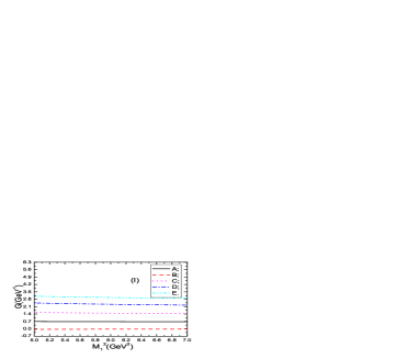
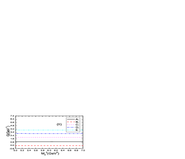
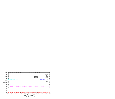
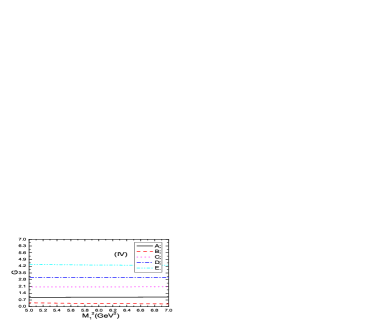
Figure 4: The hadronic coupling constants $G_{B_{c}^{*}B_{c}\Upsilon}(Q^{2})$ (I), $G_{B_{c}^{*}B_{c}J/\psi}(Q^{2})$ (II), $G_{B_{c}B_{c}\Upsilon}(Q^{2})$ (III) and $G_{B_{c}B_{c}J/\psi}(Q^{2})$ (IV) with variations of the Borel parameters $M_{1}^{2}$ or $M_{2}^{2}$ at the value $Q^{2}=1\,\rm{GeV}^{2}$. The $A$, $B$, $C$, $D$ and $E$ denote the perturbative contributions, gluon condensate contributions, leading order Coulomb-like corrections (${\mathcal{O}}(\alpha_{s}^{\mathcal{C}}/v_{s},\alpha_{s}^{\mathcal{C}}/v_{u})$), total Coulomb-like corrections and total contributions, respectively. The values of un-plotted parameters are tacitly taken as $M_{1}^{2}=6\,\rm{GeV}^{2}$ or $M_{2}^{2}=6\,\rm{GeV}^{2}$.

In Fig.4, we plot the contributions to the hadronic coupling constants $G_{B_{c}^{*}B_{c}\Upsilon}(Q^{2})$, $G_{B_{c}^{*}B_{c}J/\psi}(Q^{2})$, $G_{B_{c}B_{c}\Upsilon}(Q^{2})$ and $G_{B_{c}B_{c}J/\psi}(Q^{2})$ from different terms in the operator product expansion at the value $Q^{2}=1\,\rm{GeV}^{2}$ with variations of the Borel parameters $M_{1}^{2}$ and $M_{2}^{2}$. From the figure, we can see that the values are rather stable with variations of the Borel parameters, Borel platforms appear. The ratios among the perturbative contributions, gluon condensate contributions, leading order Coulomb-like corrections (${\mathcal{O}}(\alpha_{s}^{\mathcal{C}}/v_{s},\alpha_{s}^{\mathcal{C}}/v_{u})$), total Coulomb-like corrections, total contributions are about $(20-25)\%:(1-8)\%:50\%:(70-80)\%:1$. Although the contributions of the leading order Coulomb-like corrections are twice as large as that of the perturbative terms, the Coulomb-like corrections decrease quickly with increase of the orders of $\alpha_{s}^{\mathcal{C}}/v_{s},\alpha_{s}^{\mathcal{C}}/v_{u}$,

$$\frac{4\pi\alpha_{s}^{\mathcal{C}}}{3v}\frac{1}{1-\exp\left(-\frac{4\pi\alpha_{s}^{\mathcal{C}}}{3v}\right)} = 1+\frac{2\pi\alpha_{s}^{\mathcal{C}}}{3v}+\frac{1}{12}\left(\frac{4\pi\alpha_{s}^{\mathcal{C}}}{3v}\right)^{2}-\frac{1}{720}\left(\frac{4\pi\alpha_{s}^{\mathcal{C}}}{3v}\right)^{4}+\cdots\,,$$ (22)

where the $v$ denotes the $v_{s}$ and $v_{u}$, the operator product expansion is well convergent.

In calculations, we observe that $0.0001\leq\exp(-\frac{s_{0}}{M_{1}^{2}})\leq 0.00186$ and $0.0001\leq\exp(-\frac{u_{0}}{M_{2}^{2}})\leq 0.00186$, the contributions of high resonances and continuum states are greatly suppressed, the hadronic coupling constants $G_{B_{c}^{*}B_{c}\Upsilon}(Q^{2})$, $G_{B_{c}^{*}B_{c}J/\psi}(Q^{2})$, $G_{B_{c}B_{c}\Upsilon}(Q^{2})$ and $G_{B_{c}B_{c}J/\psi}(Q^{2})$ are not sensitive to the threshold parameters. The two criteria (pole dominance and convergence of the operator product expansion) of the QCDSR are fully satisfied. Furthermore, there exist Borel platforms to extract the numerical values of the hadronic coupling constants $G_{B_{c}^{*}B_{c}\Upsilon}(Q^{2})$, $G_{B_{c}^{*}B_{c}J/\psi}(Q^{2})$, $G_{B_{c}B_{c}\Upsilon}(Q^{2})$ and $G_{B_{c}B_{c}J/\psi}(Q^{2})$.

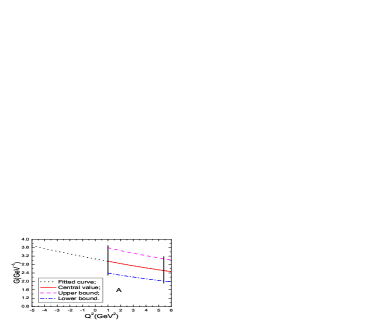
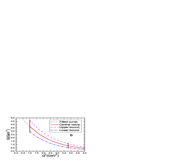
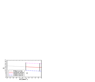
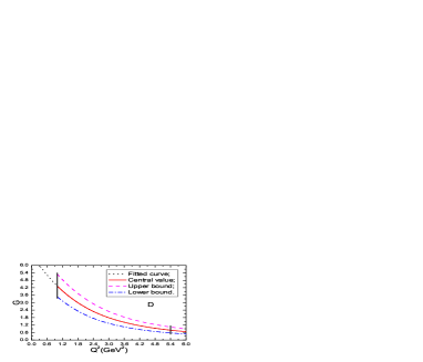
Figure 5: The hadronic coupling constants $G_{B_{c}^{*}B_{c}\Upsilon}(Q^{2})$ ($A$), $G_{B_{c}^{*}B_{c}J/\psi}(Q^{2})$ ($B$), $G_{B_{c}B_{c}\Upsilon}(Q^{2})$ ($C$) and $G_{B_{c}B_{c}J/\psi}(Q^{2})$ ($D$) with variations of the $Q^{2}=-q^{2}$, where the fitted curve denotes the central values of the fitted functions. The data between the two perpendicular lines are used to fit the parameters of the hadronic coupling constants.

The numerical values of the hadronic coupling constants $G_{B_{c}^{*}B_{c}\Upsilon}(Q^{2})$, $G_{B_{c}^{*}B_{c}J/\psi}(Q^{2})$, $G_{B_{c}B_{c}\Upsilon}(Q^{2})$ and $G_{B_{c}B_{c}J/\psi}(Q^{2})$ are shown explicitly in Figs.5, and fitted into the following analytical functions by the ${\bf\rm MINUIT}$,

$$G_{B_{c}^{*}B_{c}\Upsilon}(Q^{2}) = A\exp\left(-BQ^{2}\right)\,,$$

$$G_{B_{c}^{*}B_{c}J/\psi}(Q^{2}) = \frac{C}{1+DQ^{2}+EQ^{4}}\exp\left(-FQ^{2}\right)+H\,,$$

$$G_{B_{c}B_{c}\Upsilon}(Q^{2}) = \frac{A^{\prime}}{1+B^{\prime}Q^{2}}\,,$$

$$G_{B_{c}B_{c}J/\psi}(Q^{2}) = \frac{C^{\prime}}{1+D^{\prime}Q^{2}+E^{\prime}Q^{4}}\exp\left(-F^{\prime}Q^{2}\right)+H^{\prime}\,,$$ (23)

where

$$A = 3.0667\pm 0.43429\,\rm{GeV}^{-1}\,,$$

$$B = 0.037120\pm 0.040971\,\rm{GeV}^{-2}\,,$$

$$C = 6.1944\pm 11.883\,\rm{GeV}^{-1}\,,$$

$$D = 0.18488\pm 3.1480\,\rm{GeV}^{-2}\,,$$

$$E = 0.063663\pm 1.2289\,\rm{GeV}^{-4}\,,$$

$$F = 0.29199\pm 2.9767\,\rm{GeV}^{-2}\,,$$

$$H = 0.044515\pm 3.6666\,\rm{GeV}^{-1}\,,$$

$$A^{\prime} = 12.802\pm 0.68184\,,$$

$$B^{\prime} = 0.0078868\pm 0.016091\,\rm{GeV}^{-2}\,,$$

$$C^{\prime} = 6.6854\pm 9.7404\,,$$

$$D^{\prime} = 0.31276\pm 1.9985\,\rm{GeV}^{-2}\,,$$

$$E^{\prime} = 0.086261\pm 1.0481\,\rm{GeV}^{-4}\,,$$

$$F^{\prime} = 0.14764\pm 1.7194\,\rm{GeV}^{-2}\,,$$

$$H^{\prime} = 0.20721\pm 2.2281\,.$$ (24)

Although the uncertainties of the parameters in the $G_{B_{c}^{*}B_{c}J/\psi}(Q^{2})$, $G_{B_{c}B_{c}J/\psi}(Q^{2})$ are very large, the central values of the fitted functions $G_{B_{c}^{*}B_{c}\Upsilon}(Q^{2})$, $G_{B_{c}^{*}B_{c}J/\psi}(Q^{2})$, $G_{B_{c}B_{c}\Upsilon}(Q^{2})$ and $G_{B_{c}B_{c}J/\psi}(Q^{2})$ coincide with the central values from the QCDSR.

From the numerical values of the $G_{B_{c}^{*}B_{c}\Upsilon}(Q^{2})$, $G_{B_{c}^{*}B_{c}J/\psi}(Q^{2})$, $G_{B_{c}B_{c}\Upsilon}(Q^{2})$ and $G_{B_{c}B_{c}J/\psi}(Q^{2})$ at $Q^{2}=1\,\rm{GeV}^{2}$,

$$G_{B_{c}^{*}B_{c}\Upsilon}(Q^{2}=1\,{\rm GeV^{2}}) = 3.0\pm 0.6\,\rm{GeV}^{-1}\,,$$

$$G_{B_{c}^{*}B_{c}J/\psi}(Q^{2}=1\,{\rm GeV^{2}}) = 3.7\pm 0.8\,\rm{GeV}^{-1}\,,$$

$$G_{B_{c}B_{c}\Upsilon}(Q^{2}=1\,{\rm GeV^{2}}) = 12.8\pm 2.3\,,$$

$$G_{B_{c}B_{c}J/\psi}(Q^{2}=1\,{\rm GeV^{2}}) = 4.3\pm 0.9\,,$$ (25)

we can obtain the ratios,

$$\frac{G_{B_{c}B_{c}\Upsilon}(Q^{2}=1\,{\rm GeV^{2}})}{G_{B_{c}^{*}B_{c}\Upsilon}(Q^{2}=1\,{\rm GeV^{2}})} = 4.3\pm 1.2\,{\rm GeV}\approx m_{b}(m_{b}^{2})\,,$$

$$\frac{G_{B_{c}B_{c}J/\psi}(Q^{2}=1\,{\rm GeV^{2}})}{G_{B_{c}^{*}B_{c}J\psi}(Q^{2}=1\,{\rm GeV^{2}})} = 1.2\pm 0.4\,{\rm GeV}\approx m_{c}(m_{c}^{2})\,,$$ (26)

if the uncertainties are neglected. The ratio $\frac{G_{B_{c}B_{c}\Upsilon}(Q^{2})}{G_{B_{c}^{*}B_{c}\Upsilon}(Q^{2})}$ increases slowly with increase of the $Q^{2}$, while the ratio $\frac{G_{B_{c}B_{c}J/\psi}(Q^{2})}{G_{B_{c}^{*}B_{c}J\psi}(Q^{2})}$ increases quickly with increase of the $Q^{2}$ at the range $Q^{2}=(1-6)\,\rm{GeV}^{2}$.

In Fig.6, we extrapolate the hadronic coupling constants $G_{B_{c}^{*}B_{c}\Upsilon}(Q^{2})$, $G_{B_{c}^{*}B_{c}J/\psi}(Q^{2})$, $G_{B_{c}B_{c}\Upsilon}(Q^{2})$ and $G_{B_{c}B_{c}J/\psi}(Q^{2})$ into the deep time-like regions analytically. From the figure, we can see that the $G_{B_{c}^{*}B_{c}\Upsilon}(Q^{2})$ and $G_{B_{c}B_{c}\Upsilon}(Q^{2})$ increase monotonously with increase of the squared momentum $q^{2}=-Q^{2}$, the $G_{B_{c}^{*}B_{c}J/\psi}(Q^{2})$ also increases steadily with increase of the squared momentum $q^{2}=-Q^{2}$ and develops a shoulder at about $q^{2}=3\,\rm{GeV}^{2}$, while the $G_{B_{c}B_{c}J/\psi}(q^{2})$ develops a broad peak at about $q^{2}=2.4\,\rm{GeV}^{2}$. The fitted functions $G_{B_{c}^{*}B_{c}J/\psi}(q^{2})$ and $G_{B_{c}B_{c}J/\psi}(q^{2})$ in the time-like region $q^{2}=-Q^{2}>0$ can be reexpressed in the following forms,

$$G_{B_{c}^{*}B_{c}J/\psi}(q^{2}) = \frac{C\exp\left(Fq^{2}\right)}{1-Dq^{2}+Eq^{4}}+H=\frac{C\exp\left(Fq^{2}\right)}{\left(1-\frac{D}{2}q^{2}\right)^{2}+\left(E-\frac{D^{2}}{4}\right)q^{4}}+H\,,$$

$$G_{B_{c}B_{c}J/\psi}(q^{2}) = \frac{C^{\prime}\exp\left(F^{\prime}q^{2}\right)}{1-D^{\prime}q^{2}+E^{\prime}q^{4}}+H^{\prime}=\frac{C^{\prime}\exp\left(F^{\prime}q^{2}\right)}{\left(1-\frac{D^{\prime}}{2}q^{2}\right)^{2}+\left(E^{\prime}-\frac{D^{\prime 2}}{4}\right)q^{4}}+H^{\prime}\,,$$ (27)

with $E-\frac{D^{2}}{4}>0$ and $E^{\prime}-\frac{D^{\prime 2}}{4}>0$ for the central values of the parameters. There maybe appear peaks at the neighborhood of the values $q^{2}=\frac{1}{D}$, $\frac{2}{D}$, $\frac{1}{D^{\prime}}$ and $\frac{2}{D^{\prime}}$.

The extrapolation to deep time-like regions is highly mode-dependent and leads to systematic uncertainties for the hadronic coupling constants. In order to minimize the systematic uncertainties, we can study the vertices simultaneously by putting the $B_{c}^{*}$, $B_{c}$, $\Upsilon$ (or $J/\psi$) off-shell sequentially, then fit the hadronic coupling constants to suitable analytical functions and extrapolate them to the physical regions by requiring the on-shell values of the hadronic coupling constants coincide [8]. We postpone the tedious calculations to our next work.

Finally, we obtain the one-shell values of the $G_{B_{c}^{*}B_{c}\Upsilon}(q^{2})$, $G_{B_{c}B_{c}\Upsilon}(q^{2})$, $G_{B_{c}^{*}B_{c}J/\psi}(q^{2})$ and $G_{B_{c}B_{c}J/\psi}(q^{2})$ from the fitted functions,

$$G_{B_{c}^{*}B_{c}\Upsilon}(q^{2}=M_{\Upsilon}^{2}) = 85\,\rm{GeV}^{-1}\,,$$

$$G_{B_{c}^{*}B_{c}J/\psi}(q^{2}=M^{2}_{J/\psi}) = 20\,\rm{GeV}^{-1}\,,$$

$$G_{B_{c}B_{c}\Upsilon}(q^{2}=M_{\Upsilon}^{2}) = 44\,,$$

$$G_{B_{c}B_{c}J/\psi}(q^{2}=M^{2}_{J/\psi}) = 5\,,$$ (28)

where we retain the central values only, as the uncertainties are too large to make sense. The uncertainties originate from the uncertainties $\delta B$, $\delta C$, $\delta D$, $\delta E$, $\delta F$, $\delta B^{\prime}$, $\delta C^{\prime}$, $\delta D^{\prime}$, $\delta E^{\prime}$ and $\delta F^{\prime}$ are greatly amplified in the deep time-like regions, and much larger than the central values, while the uncertainties originate from the uncertainties $\delta A$ and $\delta A^{\prime}$ are moderate. For example, the uncertainties $\delta A=\pm 0.43429\,\rm{GeV}^{-1}$, $\delta B=\pm 0.040971\,\rm{GeV}^{-2}$, $\delta A^{\prime}=\pm 0.68184$ and $\delta B^{\prime}=\pm 0.016091\,\rm{GeV}^{-2}$ lead to $\delta G_{B_{c}^{*}B_{c}\Upsilon}(q^{2}=M_{\Upsilon}^{2})=\pm 12\,\rm{GeV}^{-1}$, $\delta G_{B_{c}^{*}B_{c}\Upsilon}(q^{2}=M_{\Upsilon}^{2})=\pm 312\,\rm{GeV}^{-1}$, $\delta G_{B_{c}B_{c}\Upsilon}(q^{2}=M_{\Upsilon}^{2})=\pm 2$ and $\delta G_{B_{c}B_{c}\Upsilon}(q^{2}=M_{\Upsilon}^{2})=\pm 213$, respectively. It is obvious that the uncertainties $\delta G_{B_{c}^{*}B_{c}\Upsilon}(q^{2}=M_{\Upsilon}^{2})=\pm 312\,\rm{GeV}^{-1}$ and $\delta G_{B_{c}B_{c}\Upsilon}(q^{2}=M_{\Upsilon}^{2})=\pm 213$ are too large to make sense. On the other hand, although the uncertainties $\delta H$ and $\delta H^{\prime}$ do not vary with the $q^{2}$, they are about ten times as large as the corresponding central values. So we only retain the central values, which are more reasonable than the uncertainties. We can take those hadronic coupling constants as basic input parameters to study final-state interactions in the heavy quarkonium decays, or calculate the absorption cross sections at the hadronic level to understand the heavy quarkonium absorptions in hadronic matter.

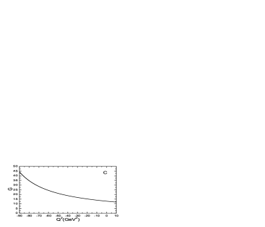
Figure 6: The central values of the hadronic coupling constants $G_{B_{c}^{*}B_{c}\Upsilon}(Q^{2})$ ($A$), $G_{B_{c}^{*}B_{c}J/\psi}(Q^{2})$ ($B$), $G_{B_{c}B_{c}\Upsilon}(Q^{2})$ ($C$) and $G_{B_{c}B_{c}J/\psi}(Q^{2})$ ($D$) extrapolated into the time-like regions.

4 Conclusion

In this article, we study the momentum dependence of the hadronic coupling constants $G_{B_{c}^{*}B_{c}\Upsilon}$, $G_{B_{c}^{*}B_{c}J/\psi}$, $G_{B_{c}B_{c}\Upsilon}$ and $G_{B_{c}B_{c}J/\psi}$ with the off-shell $\Upsilon$ and $J/\psi$ using the three-point QCDSR. Then we fit the hadronic coupling constants $G_{B_{c}^{*}B_{c}\Upsilon}(Q^{2})$, $G_{B_{c}^{*}B_{c}J/\psi}(Q^{2})$, $G_{B_{c}B_{c}\Upsilon}(Q^{2})$ and $G_{B_{c}B_{c}J/\psi}(Q^{2})$ into analytical functions, extrapolate them into the deep time-like regions, and obtain the one-shell values $G_{B_{c}^{*}B_{c}\Upsilon}(Q^{2}=-M_{\Upsilon}^{2})$, $G_{B_{c}^{*}B_{c}J/\psi}(Q^{2}=-M_{J/\psi}^{2})$, $G_{B_{c}B_{c}\Upsilon}(Q^{2}=-M_{\Upsilon}^{2})$ and $G_{B_{c}B_{c}J/\psi}(Q^{2}=-M_{J/\psi}^{2})$ for the first time, no other theoretical work on this subject exist. The hadronic coupling constants can be taken as basic input parameters in studying the heavy quarkonium absorptions in hadronic matter and final-state interactions in the heavy quarkonium hadronic decays.

Appendix

The explicit expressions of the $I_{0}^{ijn}$, $K_{0}^{ijn}$, $N_{0}^{ijn}$, $I_{10}^{ijn}$, $I_{01}^{ijn}$, $K_{10}^{ijn}$, $K_{01}^{ijn}$, $N_{10}^{ijn}$, $N_{01}^{ijn}$,

$$iI_{0}^{ijn} = B_{-p^{2}\rightarrow M_{1}^{2}}B_{-p^{\prime 2}\rightarrow M_{2}^{2}}\overline{I}_{ijn}$$ (29)

$$= \frac{(-1)^{i+j+n}i\pi^{2}}{\Gamma(i)\Gamma(j)\Gamma(n)\left(M_{2}^{2}\right)^{i}\left(M_{1}^{2}\right)^{j}\left(M^{2}\right)^{n-2}}\int_{0}^{1}d\lambda\frac{\lambda^{1-i-j}}{(1-\lambda)^{n-1}}$$

$$\exp\left\{-\frac{(1-\lambda)Q^{2}}{\lambda\left(M_{1}^{2}+M_{2}^{2}\right)}-\frac{m_{b}^{2}}{\lambda M^{2}}-\frac{m_{c}^{2}}{(1-\lambda)M^{2}}\right\}\,,$$

$$iK_{0}^{ijn} = B_{-p^{2}\rightarrow M_{1}^{2}}B_{-p^{\prime 2}\rightarrow M_{2}^{2}}\overline{K}_{ijn}$$ (30)

$$= \frac{d}{dt}\frac{(-1)^{i+j+n}i\pi^{2}}{\Gamma(i)\Gamma(j)\Gamma(n)\left(\overline{M}_{2}^{2}\right)^{i}\left(\overline{M}_{1}^{2}\right)^{j-1}\left(\overline{M}^{2}\right)^{n-2}}\int_{0}^{1}d\lambda\frac{\lambda^{1-i-j}}{(1-\lambda)^{n-1}}$$

$$\exp\left\{-\frac{(1-\lambda)Q^{2}}{\lambda\left(\overline{M}_{1}^{2}+\overline{M}_{2}^{2}\right)}-\frac{m_{b}^{2}}{\lambda\overline{M}^{2}}-\frac{m_{c}^{2}}{(1-\lambda)\overline{M}^{2}}\right\}|_{t=1,r=1}\,,$$

$$iN_{0}^{ijn} = B_{-p^{2}\rightarrow M_{1}^{2}}B_{-p^{\prime 2}\rightarrow M_{2}^{2}}\overline{N}_{ijn}$$ (31)

$$= \frac{d}{dr}\frac{(-1)^{i+j+n}i\pi^{2}}{\Gamma(i)\Gamma(j)\Gamma(n)\left(\overline{M}_{2}^{2}\right)^{i-1}\left(\overline{M}_{1}^{2}\right)^{j}\left(\overline{M}^{2}\right)^{n-2}}\int_{0}^{1}d\lambda\frac{\lambda^{1-i-j}}{(1-\lambda)^{n-1}}$$

$$\exp\left\{-\frac{(1-\lambda)Q^{2}}{\lambda\left(\overline{M}_{1}^{2}+\overline{M}_{2}^{2}\right)}-\frac{m_{b}^{2}}{\lambda\overline{M}^{2}}-\frac{m_{c}^{2}}{(1-\lambda)\overline{M}^{2}}\right\}|_{t=1,r=1}\,,$$

$$iI^{\mu}_{ijn} = B_{-p^{2}\rightarrow M_{1}^{2}}B_{-p^{\prime 2}\rightarrow M_{2}^{2}}\overline{I}^{\mu}_{ijn}$$ (32)

$$= \frac{(-1)^{i+j+n+1}i\pi^{2}}{\Gamma(i)\Gamma(j)\Gamma(n)\left(M_{2}^{2}\right)^{i}\left(M_{1}^{2}\right)^{j+1}\left(M^{2}\right)^{n-3}}\int_{0}^{1}d\lambda\frac{\lambda^{1-i-j}}{(1-\lambda)^{n-2}}$$

$$\exp\left\{-\frac{(1-\lambda)Q^{2}}{\lambda\left(M_{1}^{2}+M_{2}^{2}\right)}-\frac{m_{b}^{2}}{\lambda M^{2}}-\frac{m_{c}^{2}}{(1-\lambda)M^{2}}\right\}(p-p^{\prime})^{\mu}$$

$$+\frac{(-1)^{i+j+n}i\pi^{2}}{\Gamma(i)\Gamma(j)\Gamma(n)\left(M_{2}^{2}\right)^{i}\left(M_{1}^{2}\right)^{j}\left(M^{2}\right)^{n-2}}\int_{0}^{1}d\lambda\frac{\lambda^{2-i-j}}{(1-\lambda)^{n-1}}$$

$$\exp\left\{-\frac{(1-\lambda)Q^{2}}{\lambda\left(M_{1}^{2}+M_{2}^{2}\right)}-\frac{m_{b}^{2}}{\lambda M^{2}}-\frac{m_{c}^{2}}{(1-\lambda)M^{2}}\right\}p^{\prime\mu}$$

$$= iI_{10}^{ijn}(p-p^{\prime})^{\mu}+iI_{01}^{ijn}p^{\prime\mu}\,,$$

$$iK^{\mu}_{ijn} = B_{-p^{2}\rightarrow M_{1}^{2}}B_{-p^{\prime 2}\rightarrow M_{2}^{2}}\overline{K}^{\mu}_{ijn}$$ (33)

$$= \frac{d}{dt}\frac{(-1)^{i+j+n+1}i\pi^{2}}{\Gamma(i)\Gamma(j)\Gamma(n)\left(\overline{M}_{2}^{2}\right)^{i}\left(\overline{M}_{1}^{2}\right)^{j}\left(\overline{M}^{2}\right)^{n-3}}\int_{0}^{1}d\lambda\frac{\lambda^{1-i-j}}{(1-\lambda)^{n-2}}$$

$$\exp\left\{-\frac{(1-\lambda)Q^{2}}{\lambda\left(\overline{M}_{1}^{2}+\overline{M}_{2}^{2}\right)}-\frac{m_{b}^{2}}{\lambda\overline{M}^{2}}-\frac{m_{c}^{2}}{(1-\lambda)\overline{M}^{2}}\right\}|_{t=1,r=1}(p-p^{\prime})^{\mu}$$

$$+\frac{d}{dt}\frac{(-1)^{i+j+n}i\pi^{2}}{\Gamma(i)\Gamma(j)\Gamma(n)\left(\overline{M}_{2}^{2}\right)^{i}\left(\overline{M}_{1}^{2}\right)^{j-1}\left(\overline{M}^{2}\right)^{n-2}}\int_{0}^{1}d\lambda\frac{\lambda^{2-i-j}}{(1-\lambda)^{n-1}}$$

$$\exp\left\{-\frac{(1-\lambda)Q^{2}}{\lambda\left(\overline{M}_{1}^{2}+\overline{M}_{2}^{2}\right)}-\frac{m_{b}^{2}}{\lambda\overline{M}^{2}}-\frac{m_{c}^{2}}{(1-\lambda)\overline{M}^{2}}\right\}|_{t=1,r=1}p^{\prime\mu}$$

$$= iK_{10}^{ijn}(p-p^{\prime})^{\mu}+iK_{01}^{ijn}p^{\prime\mu}\,,$$

$$iN^{\mu}_{ijn} = B_{-p^{2}\rightarrow M_{1}^{2}}B_{-p^{\prime 2}\rightarrow M_{2}^{2}}\overline{N}^{\mu}_{ijn}$$ (34)

$$= \frac{d}{dr}\frac{(-1)^{i+j+n+1}i\pi^{2}}{\Gamma(i)\Gamma(j)\Gamma(n)\left(\overline{M}_{2}^{2}\right)^{i-1}\left(\overline{M}_{1}^{2}\right)^{j+1}\left(\overline{M}^{2}\right)^{n-3}}\int_{0}^{1}d\lambda\frac{\lambda^{1-i-j}}{(1-\lambda)^{n-2}}$$

$$\exp\left\{-\frac{(1-\lambda)Q^{2}}{\lambda\left(\overline{M}_{1}^{2}+\overline{M}_{2}^{2}\right)}-\frac{m_{b}^{2}}{\lambda\overline{M}^{2}}-\frac{m_{c}^{2}}{(1-\lambda)\overline{M}^{2}}\right\}|_{t=1,r=1}(p-p^{\prime})^{\mu}$$

$$+\frac{d}{dr}\frac{(-1)^{i+j+n}i\pi^{2}}{\Gamma(i)\Gamma(j)\Gamma(n)\left(\overline{M}_{2}^{2}\right)^{i-1}\left(\overline{M}_{1}^{2}\right)^{j}\left(\overline{M}^{2}\right)^{n-2}}\int_{0}^{1}d\lambda\frac{\lambda^{2-i-j}}{(1-\lambda)^{n-1}}$$

$$\exp\left\{-\frac{(1-\lambda)Q^{2}}{\lambda\left(\overline{M}_{1}^{2}+\overline{M}_{2}^{2}\right)}-\frac{m_{b}^{2}}{\lambda\overline{M}^{2}}-\frac{m_{c}^{2}}{(1-\lambda)\overline{M}^{2}}\right\}|_{t=1,r=1}p^{\prime\mu}$$

$$= iN_{10}^{ijn}(p-p^{\prime})^{\mu}+iN_{01}^{ijn}p^{\prime\mu}\,,$$

where

$$M^{2} = \frac{M_{1}^{2}M_{2}^{2}}{M_{1}^{2}+M_{2}^{2}}\,,$$

$$\overline{M}^{2} = \frac{\overline{M}_{1}^{2}\overline{M}_{2}^{2}}{\overline{M}_{1}^{2}+\overline{M}_{2}^{2}}\,,$$

$$\overline{M}_{1}^{2} = tM_{1}^{2}\,,$$

$$\overline{M}_{2}^{2} = rM_{2}^{2}\,,$$ (35)

and the $B_{-p^{2}\rightarrow M_{1}^{2}}B_{-p^{\prime 2}\rightarrow M_{2}^{2}}$ denotes the double Borel transform.

References

[1] T. Matsui and H. Satz, Phys. Lett. B178 (1986) 416.
[2] R. Vogt, Phys. Rept. 310 (1999) 197;
R. Rapp, D. Blaschke and P. Crochet, Prog. Part. Nucl. Phys. 65 (2010) 209.
[3] P. Braun-Munzinger and J. Stachel, Phys. Lett. B490 (2000) 196;
R. L. Thews, M. Schroedter and J. Rafelski, Phys. Rev. C63 (2001) 054905;
L. Grandchamp and R. Rapp, Phys. Lett. B523 (2001) 60;
L. Grandchamp and R. Rapp, Nucl. Phys. A709 (2002) 415;
A. Capella, L. Bravina, E. G. Ferreiro, A. B. Kaidalov, K. Tywoniuk and E. Zabrodin, Eur. Phys. J. C58 (2008) 437.
[4] E. G. Ferreiro, F. Fleuret, J. P. Lansberg and A. Rakotozafindrabe, Phys. Lett. B680 (2009) 50;
R. Vogt, Phys. Rev. C81 (2010) 044903;
A. Rakotozafindrabe, E. G. Ferreiro, F. Fleuret, J. P. Lansberg and N. Matagne, Nucl. Phys. A855 (2011) 327.
[5]
S. G. Matinyan and B. Muller, Phys. Rev. C58 (1998) 2994;
K. L. Haglin, Phys. Rev. C61 (2000) 031902;
Z. W. Lin and C. M. Ko, Phys. Rev. C62 (2000) 034903;
A. Sibirtsev, K. Tsushima and A. W. Thomas, Phys. Rev. C63 (2001) 044906;
Z. W. Lin and C. M. Ko, Phys. Lett. B503 (2001) 104.
[6] R. Casalbuoni, A. Deandrea, N. Di Bartolomeo, R. Gatto, F. Feruglio and G. Nardulli, Phys. Rept. 281 (1997) 145;
X. Liu, B. Zhang and S. L. Zhu, Phys. Lett. B645 (2007) 185;
C. Meng and K. T. Chao, Phys. Rev. D78 (2008) 074001;
F. K. Guo, C. Hanhart, G. Li, U. G. Meissner and Q. Zhao, Phys. Rev. D83 (2011) 034013.
[7] F. S. Navarra, M. Nielsen, M. E. Bracco, M. Chiapparini and C. L. Schat, Phys. Lett. B489 (2000) 319;
M. E. Bracco, M. Chiapparini, A. Lozea, F. S. Navarra and M. Nielsen, Phys. Lett. B521 (2001) 1;
F. S. Navarra, M. Nielsen and M. E. Bracco, Phys. Rev. D65 (2002) 037502;
R. D. Matheus, F.S. Navarra, M. Nielsen and R. Rodrigues da Silva, Phys. Lett. B541 (2002) 265;
R. Rodrigues da Silva, R. D. Matheus, F. S. Navarra and M. Nielsen, Braz. J. Phys. 34 (2004) 236;
M. E. Bracco, M. Chiapparini, F. S. Navarra and M. Nielsen, Phys. Lett. B605 (2005) 326;
M. E. Bracco, A. Cerqueira, M. Chiapparini, A. Lozea and M. Nielsen, Phys. Lett. B641 (2006) 286;
M. E. Bracco, M. Chiapparini, F. S. Navarra and M. Nielsen, Phys. Lett. B659 (2008) 559;
M. E. Bracco and M. Nielsen, Phys. Rev. D82 (2010) 034012;
B. O. Rodrigues, M. E. Bracco, M. Nielsen and F. S. Navarra, Nucl. Phys. A852 (2011) 127;
K. Azizi and H. Sundu, J. Phys. G38 (2011) 045005;
H. Sundu, J.Y. Sungu, S. Sahin, N. Yinelek and K. Azizi, Phys. Rev. D83 (2011) 114009;
A. Cerqueira, Jr, B. O. Rodrigues and M. E. Bracco, Nucl. Phys. A874 (2012) 130;
C. Y. Cui, Y. L. Liu and M. Q. Huang, Phys. Lett. B707 (2012) 129;
C. Y. Cui, Y. L. Liu and M. Q. Huang, Phys. Lett. B711 (2012) 317.
[8]
M. E. Bracco, M. Chiapparini, F. S. Navarra and M. Nielsen, Prog. Part. Nucl. Phys. 67 (2012) 1019.
[9]
P. Colangelo, F. De Fazio, G. Nardulli, N. Di Bartolomeo and R. Gatto, Phys. Rev. D52 (1995) 6422;
T. M. Aliev, N. K. Pak and M. Savci, Phys. Lett. B390 (1997) 335;
P. Colangelo and F. De Fazio, Eur. Phys. J. C4 (1998) 503;
Y. B. Dai and S. L. Zhu, Phys. Rev. D58 (1998) 074009;
S. L. Zhu and Y. B. Dai, Phys. Rev. D58 (1998) 094033;
A. Khodjamirian, R. Ruckl, S. Weinzierl and O. I. Yakovlev, Phys. Lett. B457 (1999) 245;
Z. H. Li, T. Huang, J. Z. Sun and Z. H. Dai, Phys. Rev. D65 (2002) 076005;
H. c. Kim and S. H. Lee, Eur. Phys. J. C22 (2002) 707;
D. Becirevic, J. Charles, A. LeYaouanc, L. Oliver, O. Pene and J. C. Raynal, JHEP 0301 (2003) 009;
Z. G. Wang and S. L. Wan, Phys. Rev. D73 (2006) 094020;
Z. G. Wang and S. L. Wan, Phys. Rev. D74 (2006) 014017;
Z. G. Wang, Eur. Phys. J. C52 (2007) 553;
Z. G. Wang, Nucl. Phys. A796 (2007) 61;
Z. G. Wang, J. Phys. G34 (2007) 753;
Z. G. Wang, Phys. Rev. D77 (2008) 054024;
Z. G. Wang and Z. B. Wang, Chin. Phys. Lett. 25 (2008) 444;
Z. H. Li, W. Liu and H. Y. Liu, Phys. Lett. B659 (2008) 598.
[10] M. A. Shifman, A. I. Vainshtein and V. I. Zakharov, Nucl. Phys. B147 (1979) 385, 448.
[11] L. J. Reinders, H. Rubinstein and S. Yazaki, Phys. Rept. 127 (1985) 1.
[12] P. Colangelo and A. Khodjamirian, arXiv:hep-ph/0010175.
[13] Z. G. Wang, Eur. Phys. J. A49 (2013) 131.
[14] Z. G. Wang, Eur. Phys. J. C73 (2013) 2559.
[15] Z. G. Wang, Commun. Theor. Phys. 61 (2014) 81.
[16] B .L. Ioffe and A. V. Smilga, Nucl. Phys. B216 (1983) 373;
D. S. Du, J. W. Li and M. Z. Yang, Eur. Phys. J. C37 (2004) 173.
[17] V. V. Kiselev, A. K. Likhoded and A. I. Onishchenko, Nucl. Phys. B569 (2000) 473.
[18] V. V. Kiselev, Int. J. Mod. Phys. A11 (1996) 3689;
V. V. Kiselev, A. E. Kovalsky and A. K. Likhoded, Nucl. Phys. B585 (2000) 353.
[19] V. V. Kiselev, Central Eur. J. Phys. 2 (2004) 523.
[20] J. Beringer et al, Phys. Rev. D86 (2012) 010001.
[21] A. A. Penin, A. Pineda, V. A. Smirnov and M. Steinhauser, Phys. Lett. B593 (2004) 124.
[22] S. Narison, Phys. Lett. B693 (2010) 559; S. Narison, Phys. Lett. B706 (2012) 412;
S. Narison, Phys. Lett. B707 (2012) 259.