Near the sill of the conformal window:
gauge theories with fermions in two-index representations

Abstract

We apply Schrödinger functional methods to two gauge theories with fermions in two-index representations: the SU(3) theory with $N_{f}=2$ adjoint fermions, and the SU(4) theory with $N_{f}=6$ fermions in the two-index antisymmetric representation. Each theory is believed to lie near the bottom of the conformal window for its respective representation. In the SU(3) theory we find a small beta function in strong coupling but we cannot confirm or rule out an infrared fixed point. In the SU(4) theory we find a hint of walking—a beta function that approaches the axis and then turns away from it. In both theories the mass anomalous dimension remains small even at the strongest couplings, much like the theories with fermions in the two-index symmetric representation investigated earlier.

I Introduction

The extension of lattice gauge methods to theories beyond QCD has been largely aimed at determining the infrared properties of these theories Neil:2012cb ; Giedt:2012it . For a given gauge group, one varies the number $N_{f}$ of fermion flavors to try to find the conformal window, the range of $N_{f}$ where the theory is scale invariant at large distances. Below this window the theory confines and breaks global symmetries, much like QCD; the most interesting range of $N_{f}$ is the borderline area Holdom:1981rm ; Yamawaki:1985zg ; Hill:2002ap . In a further departure from QCD, one can put the fermions in a color representation other than the fundamental. This opens a large arena for exploration Sannino:2004qp ; Hong:2004td ; Dietrich:2006cm .

In this paper we analyze two gauge theories: the SU(3) gauge theory with $N_{f}=2$ Dirac fermions in the adjoint representation, and the SU(4) theory with $N_{f}=6$ Dirac fermions in the sextet, which is an antisymmetric tensor with two indices. For the SU(3)/adjoint theory, $N_{f}=2$ is the only value that is interesting, in that the coefficients $b_{1},b_{2}$ of the one- and two-loop terms in the beta function,

$$\beta(g^{2})=-b_{1}\frac{g^{4}}{16\pi^{2}}-b_{2}\frac{g^{6}}{(16\pi^{2})^{2}}+\cdots,$$ (1)

satisfy

$$b_{1}>0,\qquad b_{2}<0.$$ (2)

The two-loop beta function thus possesses an infrared-stable fixed point (IRFP) Caswell:1974gg ; Banks:1981nn , which invites non-perturbative confirmation. As for the SU(4)/sextet theory, the condition (2) offers a wider range of $N_{f}$ for study (see Table 1). Approximate solutions of the Schwinger–Dyson equations Appelquist:1988yc ; Cohen:1988sq indicate that the $N_{f}=6,7$ theories lie below the sill of the conformal window while $N_{f}=8$ lies just above (see Ref. Dietrich:2006cm ). Allowing that all three theories invite study, we chose to start with $N_{f}=6$ so as to approach the conformal window from below.

Table 1: Coefficients of the two-loop beta function for the SU(3)/adjoint and SU(4)/sextet theories, and location of its zero $g_{*}^{2}$. For comparison we list the quantities for borderline theories with two-index symmetric representations.

	$N_{f}$	$b_{1}$	$b_{2}$	$g_{*}^{2}$
SU(3)/adjoint	2	3	$-90$	$5.26$
SU(4)/sextet	6	$6\frac{2}{3}$	$-38\frac{2}{3}$	$27.2$
	7	$5\frac{1}{3}$	$-75\frac{1}{3}$	$11.2$
	8	4	$-112$	$5.6$
SU(2)/triplet	2	2	$-40$	$7.9$
SU(3)/sextet	2	$4\frac{1}{3}$	$-64\frac{2}{3}$	$10.6$
SU(4)/decuplet	2	$6\frac{2}{3}$	$-86\frac{2}{3}$	$12.1$

We apply the method of the Schrödinger functional (SF) to calculate the running coupling of the theories at hand, and thus their beta functions. This method was developed Luscher:1992an ; Luscher:1993gh ; Sint:1993un ; Sint:1995ch ; Jansen:1998mx ; DellaMorte:2004bc to study small-$N_{f}$ QCD, whose coupling runs fast in evolving from short to long distance scales. While we use the same definition of the running coupling, we analyze the results with methods that we have found useful for conformal and near-conformal theories, where the coupling runs very slowly. We developed these methods in the course of our work on three gauge theories that lie near the bottom of the conformal window: the SU(2) DeGrand:2011qd , SU(3) Shamir:2008pb ; DeGrand:2010na ; DeGrand:2012yq , and SU(4) DeGrand:2012qa theories, all with $N_{f}=2$ fermions in the respective two-index symmetric representations (2ISR) of color.

The present study takes us to new two-index representations—the adjoint and the antisymmetric. Our SF analysis, even before extrapolation to the continuum limit, is inconclusive regarding the existence of an IRFP in both theories we study. The extrapolation of our data to the continuum is difficult. The resulting error bars are on the same scale as the one-loop beta function, and so we cannot tell whether the beta function for each theory crosses zero. It is possible that it approaches zero and then runs off to negative values, behavior known as walking. The SU(4)/sextet theory, in particular, shows a hint of this behavior, but with large error bars.

As in our work on the 2ISR models, we are able to give more precise results for $\gamma_{m}$, the anomalous dimension of the fermion mass, defined as usual through the scaling behavior of $\bar{\psi}\psi$. This is calculated as a byproduct of the SF calculation Sint:1998iq ; Capitani:1998mq ; DellaMorte:2005kg ; Bursa:2009we . We find, as in the other theories, that as $g^{2}$ is increased, $\gamma_{m}$ deviates downwards from the one-loop curve and levels off below 0.4 in both the SU(3) and the SU(4) theories. This result is robust under continuum extrapolation.

The levelling-off of $\gamma_{m}(g)$ in these theories and in the 2ISR theories is a remarkable result. No such behavior has ever appeared in perturbation theory. As we have noted before, the existence of a global bound on $\gamma_{m}$ is evidently invariant under any redefinition $g\to g^{\prime}(g)$, that is, it is entirely scheme-independent.

The SU(3) lattice gauge theory with two adjoint fermions has attracted attention as an extension of QCD in which the dynamical scales of confinement and of chiral symmetry breaking might be separated. Following early quenched Kogut:1984sb and unquenched Gerstenmayer:1989qw studies, Karsch and Lütgemeier Karsch:1998qj carried out an extensive study of the $N_{f}=2$ theory with staggered fermions. They found clear evidence for separate finite-temperature phase transitions. The nature of the chiral phase transition, which should follow the scheme Peskin:1980gc $\textrm{SU}(4)\to\textrm{SO}(4)$, was investigated in Refs. Basile:2004wa ; Engels:2005te . The theory has also served as a laboratory for studying monopole condensation Cossu:2008wh and finite-size phase transitions Unsal:2007jx ; Cossu:2009sq .

The finite-temperature transitions found in the above work would seem to rule out IR conformality in the SU(3)/adjoint theory. After all, an IR conformal theory would have no scale from which one could construct a zero-temperature chiral condensate, a string tension, or a transition temperature. The evidence offered so far, however, is inconclusive. The results cited above were obtained in studies on finite-temperature lattices with only one value of $n_{\tau}$, the number of sites in the Euclidean time direction. When $n_{\tau}=4$, say, the lattice spacing itself sets a scale for the temperature so that a transition occurs at some bare coupling $g_{0}^{*}$. A true test of confinement vs. conformality requires varying $n_{\tau}$ to see the behavior of $g_{0}^{*}(n_{\tau})$. This will determine whether, in the continuum limit, the transition temperature reaches a finite limit or tends to zero. Such a program has been attempted for the SU(3)/triplet theory with various $N_{f}$ Deuzeman:2008sc ; Miura:2011mc ; Cheng:2011ic ; Deuzeman:2012ee ; Miura:2012zqa and for the SU(3)/sextet theory Kogut:2010cz ; Kogut:2011ty ; Kogut:2011bd ; Sinclair:2012fa , and it is fraught with difficulties.

The SU(4)/sextet theory has not been studied on the lattice before. It stands out in Table 1. For $N_{f}=6$, the zero of the two-loop beta function occurs at $g_{*}^{2}\simeq 27.2$. This is a much stronger coupling than in the other borderline theories listed in the table. In the 2ISR theories DeGrand:2011qd ; Shamir:2008pb ; DeGrand:2010na ; DeGrand:2012yq ; DeGrand:2012qa as well as in the SU(3)/adjoint theory (see below), we found that the nonperturbative beta function follows the two-loop form fairly closely out to its zero. Clearly the two-loop beta function cannot be trusted out to $g^{2}=27$, and in fact we will show below that the calculated beta function deviates and approaches zero at a much weaker coupling.

We review the choice of lattice action and describe our simulations in Sec. II. We present the analysis of the running coupling and the beta function in both theories in Sec. III, and the mass anomalous dimension in Sec. IV. We conclude with a summary of our results and a discussion of the difficulties encountered.

II Lattice action, phase diagram, and ensembles

Our fermion action $\bar{\psi}D_{F}\psi$ is the conventional Wilson action, supplemented by a clover term Sheikholeslami:1985ij with coefficient $c_{\text{SW}}=1$ Shamir:2010cq . The gauge links in the fermion action are fat link variables $V_{\mu}(x)$. The fat links are the normalized hypercubic (nHYP) links of Refs. Hasenfratz:2001hp ; Hasenfratz:2007rf with weighting parameters $\alpha_{1}=0.75$, $\alpha_{2}=0.6$, $\alpha_{3}=0.3$, subsequently promoted to the fermions’ representation.

As we found in our previous work DeGrand:2012qa ; DeGrand:2012yq , it is useful to generalize the pure gauge part of the action beyond the usual plaquette term to include a term built out of fat links. Thus,

$$S_{G} = -\frac{\beta}{2N}\sum_{\mu\neq\nu}{\rm Re\,}{\rm Tr}\,U_{\mu}(x)U_{\nu}(x+\hat{\mu})U_{\mu}^{\dagger}(x+\hat{\nu})U_{\nu}^{\dagger}(x)$$

$$-\frac{\beta^{\prime}}{2d_{f}}\sum_{\mu\neq\nu}{\rm Re\,}{\rm Tr}\,V_{\mu}(x)V_{\nu}(x+\hat{\mu})V_{\mu}^{\dagger}(x+\hat{\nu})V_{\nu}^{\dagger}(x).$$

$N=3,4$ is the number of colors while $d_{f}$ ($=8,6$, respectively) is the dimension of the fermion representation.

The reason for adding the $\beta^{\prime}$ term can be found in the phase diagram sketched in Fig. 1 Iwasaki:1991mr ; Iwasaki:2003de ; Nagai:2009ip . We verified this phase diagram in the SU(3)/sextet theory DeGrand:2010na ; DeGrand:2008kx and in the SU(2)/triplet theory DeGrand:2011qd (where part of the phase boundary is a second-order transition). For the two theories at hand, we discovered the same structure in the course of determining the $\kappa_{c}(\beta)$ curve. Our SF calculations are, in principle, carried out on the $\kappa_{c}(\beta)$ line, where $m_{q}=0$, to the right of the point marked $(\beta_{1},\kappa_{1})$. Our goal is to reach as strong a running coupling as possible, by pushing to strong bare couplings. At strong coupling, however, we encounter either the phase transition shown or impossibly low acceptance due to roughness of the typical gauge configuration. Adjusting $\beta^{\prime}$ can help push these limitations off towards stronger coupling. An exploration of the $(\beta,\beta^{\prime})$ plane similar to that described in Ref. DeGrand:2012qa led us to set $\beta^{\prime}=0.5$ in the SU(4) theory. In the SU(3) theory, on the other hand, we found no advantage in adjusting $\beta^{\prime}$ away from zero. Any other choice decreased the range of accessible couplings. See the Appendix for more information.

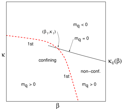
Figure 1: Presumed phase diagram for both the SU(3)/adjoint and SU(4)/sextet theories, for $|\beta^{\prime}|$ not too large. The first-order phase boundary, as well as the $\kappa_{c}(\beta)$ curve, shifts with $\beta^{\prime}$; the SF coupling $g$ is determined along the $\kappa_{c}$ curve, and it, too, depends on $\beta^{\prime}$.

We determine the critical hopping parameter $\kappa_{c}=\kappa_{c}(\beta)$ by setting to zero the quark mass $m_{q}$, as defined by the unimproved axial Ward identity. $m_{q}$ is of course volume-dependent on small lattices. Ideally, we would like to fix $\kappa_{c}$ so that $m_{q}\to 0$ in the infinite-volume limit. For clear practical reasons, we instead do the determination in relatively short runs on lattices of size $L=12a$. In our work on the SU(2)/adjoint theory DeGrand:2011qd , we addressed the concern that an extrapolation of $m_{q}$ to infinite volume might show that the $L\to\infty$ limit is far from massless. The problem is potentially serious only at the strongest couplings, and we showed that, even there, adjustment of $\kappa$ to make $m_{q}$ acceptably small does not affect the results for the $\beta$ function or the anomalous dimension $\gamma_{m}$.

In the SU(3)/adjoint theory, on the other hand, the determination of $\kappa_{c}$ runs into trouble at the strongest couplings, $\beta=3.8$ and 3.9, and this time the problem lies in the smallest lattices. We refer again to Fig. 1. Both the first-order phase boundary and the $\kappa_{c}(\beta)$ curve shift with volume. We show in Fig. 2 the data for $m_{q}(\kappa)$ for the various volumes at the two strongest bare couplings, $\beta=3.8$ and 3.9.

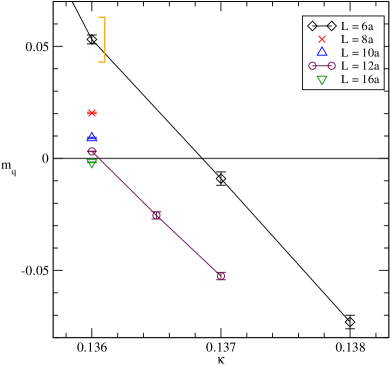
Figure 2: $m_{q}(\kappa)$, determined from the axial Ward identity, for the strongest couplings studied in the SU(3)/adjoint theory. Left: $\beta=3.8$. Right: $\beta=3.9$. The square brackets indicate measurements in a metastable state.

For each coupling we fix $\kappa_{c}$ by demanding $m_{q}=0$ for $L=12a$. At $\beta=3.8$, this fixes $\kappa_{c}=0.1369$. As can be seen in the figure, the values of $m_{q}$ at this $\kappa$ for $L=10a$ and $L=8a$ are nonzero and positive. This would hold as well for $L=6a$, except that for $L=6a$ the phase boundary in Fig. 1 has moved up past $\kappa=0.1369$ so that we find ourselves in the confining phase. It is impossible to simulate for $L=6a$ at the $\kappa_{c}$ determined at $L=12a$. It is worth noting that there is still a value of $\kappa$ at which $m_{q}$ crosses zero for $L=6a$; like the phase boundary, it has shifted upwards. The bottom line is that we are prevented from simulating on the $L=6a$ lattice at $\kappa_{c}$.

For $\beta=3.9$ the situation is the same, except that for $L=6a$ at $\kappa=\kappa_{c}=0.1360$ we succeeded in simulating in a short run in the metastable state that is non-confining. (This is the origin of the bracketed point in the figure on the right.) The lifetime of the metastable state, however, was too short to make it useful for an SF measurement. Going back to $\beta=3.8$, we found in fact that for $L=8a$ as well, the non-confining state is metastable at $\kappa_{c}$. In this case, however, we were able to run a very long simulation and thus to make a useful determination of the SF observables.

We stress that the metastability issue on the small volumes at $\beta=3.8$ and 3.9 is distinct from what happens to the left of $(\beta_{1},\kappa_{1})$ in Fig. 1. The strong-coupling part of the phase boundary is a place where $m_{q}$ flips sign discontinuously, and there is no equilibrium measurement that will give $m_{q}=0$ for any volume DeGrand:2011qd . At $\beta=3.8$ and 3.9, on the other hand, each lattice size allows a value of $\kappa$ where $m_{q}=0$. The fact that this $\kappa$ shifts with $L$ does not pose a special problem; the shift in the phase boundary does pose a practical problem in preventing simulation at a given $\kappa$ for small volumes. We overcame this in the case of $(\beta=3.8,L=8a)$, however, and so we make use of the data here even though the state is metastable.

Our tables for the SU(3)/adjoint theory are thus missing entries for $L=6a$ at the two strongest couplings. This problem did not appear in the SU(4)/sextet theory. Moreover, we did not run simulations for $L=16a$ at the weakest coupling in either theory.

As before, we employed the hybrid Monte Carlo (HMC) algorithm in our simulations. The molecular dynamics integration was accelerated with an additional heavy pseudo-fermion field as suggested by Hasenbusch Hasenbusch:2001ne , multiple time scales Urbach:2005ji , and a second-order Omelyan integrator Takaishi:2005tz . The ensembles generated for the two theories are listed in Tables 2 and 3. For the SU(3) theory, each ensemble for $L\geq 10a$ was divided into four streams, with the requirement that the observables from the four streams be consistent to a low $\chi^{2}$. For the SU(4) theory this was done for all the ensembles, including $L=6a,8a$.

The SU(3) theory was particularly difficult to simulate in its strong coupling region, requiring short trajectories and producing long autocorrelation times, which in turn resulted in slow convergence of the separate streams. For several values of $(\beta,L)$, we were unable to satisfy our consistency test of $\chi^{2}<6$ for 3 degrees of freedom, in one observable or another, among the four streams. In most of these cases, however, we saw a steady improvement with the length of the run. Moreover, we found that the high $\chi^{2}$ was caused by one stream out of the four; dropping this stream in favor of the majority resulted in a change of the mean that was less than $1\sigma$. We decided therefore to deem these results statistically consistent. The only exception arose at $\beta=3.8$ for $L=16a$, the largest volume at the strongest coupling. Here an outlying stream resulted in $\chi^{2}=16/3$ dof in the result for $Z_{P}$, with no sign of improvement as the streams grew longer. We were left with no choice but to omit this stream from the final average, resulting in a shift by $2.5\sigma$. This one result for $Z_{P}$ is thus less reliable than the others and we mark it so in the following.

The tables show that the SU(4) theory reached reasonable error bars with much shorter simulations. There were no special problems with $\chi^{2}$ among the streams once they had become long enough.

Table 2: Ensembles generated at the bare couplings $(\beta,\kappa_{c})$, on lattice sizes $L$, for the SU(3)/adjoint theory. For this theory no fat-plaquette term was added to the action. Listed are the total number of trajectories for all streams at given $(\beta,L)$, the trajectory length, and the HMC acceptance.

$\beta$	$\kappa_{c}$	$L/a$	trajectories	trajectory	acceptance
			(thousands)	length
3.8	0.1369	8	21	1.0	0.46
		10	62	0.5	0.65
		12	80	0.5	0.64
		16	88	0.4	0.43
3.9	0.136	8	37	1.0	0.68
		10	76	0.5	0.77
		12	133	0.5	0.72
		16	100	0.4	0.57
4.1	0.13454	6	26	1.0	0.85
		8	18	1.0	0.67
		10	38	0.5	0.87
		12	48	0.5	0.84
		16	26	0.5	0.70
4.5	0.13172	6	16	1.0	0.99
		8	9	1.0	0.97
		10	13	1.0	0.94
		12	19	1.0	0.88
		16	10	1.0	0.81
5.0	0.1295	6	17	1.0	0.99
		8	8	1.0	0.99
		10	13	1.0	0.99
		12	32	1.0	0.97

Table 3: Ensembles generated at the bare couplings $(\beta,\kappa_{c})$, on lattice sizes $L$, for the SU(4)/sextet theory. For this theory a fat-plaquette term was added to the action with coefficient $\beta^{\prime}=0.5$. Columns as in Table 2.

$\beta$	$\kappa_{c}$	$L/a$	trajectories	trajectory	acceptance
			(thousands)	length
5.5	0.13398	6	8	1.0	0.74
		8	8	0.5	0.79
		10	16	0.5	0.77
		12	48	0.5	0.57
		16	17	0.5	0.38
6.0	0.13315	6	8	1.0	0.64
		8	8	1.0	0.48
		10	8	0.5	0.45
		12	10	0.5	0.73
		16	16	0.5	0.57
7.0	0.13120	6	8	1.0	0.92
		8	8	1.0	0.84
		10	8	1.0	0.67
		12	16	1.0	0.47
		16	11	0.5	0.82
8.0	0.12933	6	8	1.0	0.98
		8	8	1.0	0.96
		10	8	1.0	0.93
		12	16	1.0	0.65
		16	16	0.5	0.86
10.0	0.12702	6	8	1.0	0.99
		8	8	1.0	0.99
		10	8	1.0	0.99
		12	8	1.0	0.97

III The running coupling and the beta function

We compute the running coupling in the SF method exactly as described in our previous papers. We impose Dirichlet boundary conditions at the time slices $t=0,L,$ and measure the response of the quantum effective action. The coupling emerges from a measurement of the derivative of the action with respect to a parameter $\eta$ in the boundary gauge field,

$$\frac{K}{g^{2}(L)}=\left.\left\langle\frac{\partial S_{G}}{\partial\eta}-{\rm tr}\,\left(\frac{1}{D_{F}^{\dagger}}\;\frac{\partial(D_{F}^{\dagger}D_{F})}{\partial\eta}\;\frac{1}{D_{F}}\right)\right\rangle\right|_{\eta=0}.$$ (4)

The boundary conditions we use for each theory are copied from other theories with the same gauge group. For the SU(3)/adjoint model, see our paper on the SU(3)/sextet theory DeGrand:2010na ; for the SU(4)/sextet theory see our paper on the SU(4)/decuplet theory DeGrand:2012qa . The constant $K=12\pi$ emerges directly from the classical continuum action.

We list the calculated running couplings for the SU(3) theory in Table 4 and for the SU(4) theory in Table 5; they are plotted in Figs. 3 and 4, respectively.

Table 4: Running coupling measured in the SU(3)/adjoint theory.

$\beta$	$1/g^{2}$
	$L=6a$	$L=8a$	$L=10a$	$L=12a$	$L=16a$
3.8	–	0.1343(32)	0.1387(29)	0.1438(31)	0.1387(55)
3.9	–	0.1561(26)	0.1576(28)	0.1558(27)	0.1568(45)
4.1	0.2059(22)	0.2031(40)	0.2106(40)	0.2000(43)	0.1989(67)
4.5	0.2954(26)	0.2959(40)	0.2838(45)	0.2765(43)	0.2826(69)
5.0	0.4016(27)	0.3993(54)	0.3953(44)	0.3900(34)	–

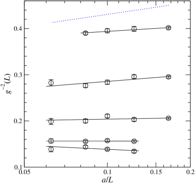
Figure 3: Running coupling $1/g^{2}$ vs. $a/L$ in the SU(3)/adjoint theory (Table 4). Top to bottom: $\beta=5.0,$ 4.5, 4.1, 3.9, 3.8. The straight lines are linear fits [Eq. (6)] to each set of points at given $\beta$; the slope gives the beta function. The dotted line shows the expected slope from one-loop running.

Table 5: Running coupling measured in the SU(4)/sextet theory.

$\beta$	$1/g^{2}$
	$L=6a$	$L=8a$	$L=10a$	$L=12a$	$L=16a$
5.5	0.1244(21)	0.1225(40)	0.1297(32)	0.1213(22)	0.1120(60)
6.0	0.1675(26)	0.1676(38)	0.1626(42)	0.1659(45)	0.1592(54)
7.0	0.2849(27)	0.2692(32)	0.2642(45)	0.2448(45)	0.2581(66)
8.0	0.4193(27)	0.3947(42)	0.3905(27)	0.3777(40)	0.3628(69)
10.0	0.7214(32)	0.7000(42)	0.6729(53)	0.6621(58)	–

Figure 4: Same as Fig. 3, but for the SU(4)/sextet theory (Table 5). Top to bottom: $\beta=10.0,$ 8.0, 7.0, 6.0, 5.5.

We define the beta function $\tilde{\beta}(u)$ for $u\equiv 1/g^{2}$ as

$$\tilde{\beta}(u)\equiv\frac{d(1/g^{2})}{d\log L}=2\beta(g^{2})/g^{4}=2u^{2}\beta(1/u).$$ (5)

As discussed in Ref. DeGrand:2011qd , the slow running of the coupling suggests extracting the beta function at each $(\beta,\kappa_{c})$ from a linear fit of the inverse coupling

$$u(L)=c_{0}+c_{1}\log\frac{L}{8a}\ .$$ (6)

With this parametrization, $c_{0}$ gives the inverse coupling $u(L=8a)$, while $c_{1}$ is an estimate for the beta function $\tilde{\beta}$ at this coupling.

For a first look, we fit the data points for all $L$ to extract the slopes at the given bare parameters, ignoring discretization errors that must be inherent in the smallest lattices. These fits are shown in Figs. 3 and 4. Values of the beta function $\tilde{\beta}(u)$ obtained from these fits are plotted as a function of $u(L=8a)$ in Fig. 5.

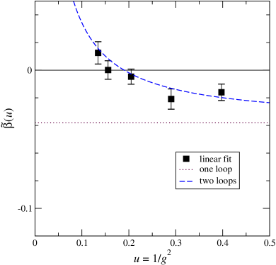
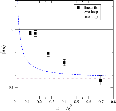
Figure 5: Beta function $\tilde{\beta}(u)$ of the SU(3)/adjoint theory (left) and the SU(4)/sextet theory (right), plotted as a function of $u(L=8a)$. Results are extracted from the linear fits (6), as shown in Figs. 3 and 4, respectively. Plotted curves are the one-loop (dotted line) and two-loop (dashed line) beta functions. No correction has been made for discretization errors.

Also shown are the one- and two-loop approximations from the expansion (see Table 1)

$$\tilde{\beta}(u)=-\frac{2b_{1}}{16\pi^{2}}-\frac{2b_{2}}{(16\pi^{2})^{2}}\frac{1}{u}+\cdots.$$ (7)

The plotted points for the SU(3) theory follow the two-loop curve closely, including its zero crossing. This would imply an IRFP, but at low significance since the leftmost point is but $1.5\sigma$ above zero. (We will see also that continuum extrapolation drives the point negative.) In the case of the SU(4) theory, we see a large deviation from the two-loop curve in strong coupling, even tending towards a zero crossing but not quite getting there. In both cases, one might be tempted to draw a smooth curve that crosses zero, but one could also draw a curve that approaches zero and then falls away, which is just the conjectured behavior for walking.

In Ref. DeGrand:2012yq we introduced a method for extrapolating lattice results to the continuum limit when a theory runs slowly. The key observation is that when a theory is almost conformal, the finite lattice corrections will not depend separately on $a$ and on $L$ but only on the ratio $(a/L)$. Then successive elimination of the lattices with coarsest lattice spacing $a$ is equivalent to dropping the smallest lattice sizes $L$. We calculated $\tilde{\beta}(u)$ above by linear fits [Eq. (6)] to $1/g^{2}$ measured on lattices of size $L_{1}<L_{2}<\ldots<L_{N}$. The results for this first fit are the coefficients $c_{0}\equiv c_{0}^{(1)}$ and $c_{1}\equiv c_{1}^{(1)}$. We can obtain results closer to the continuum limit by dropping the smallest lattice $L_{1}$ from consideration, whereupon a linear fit gives $c_{0}^{(2)},c_{1}^{(2)}$. Dropping the two smallest lattices gives $c_{0}^{(3)},c_{1}^{(3)}$, and so forth. Each $c_{1}^{(n)}$ is an approximant to $\tilde{\beta}(u)$ associated with $L=L_{n}$, the smallest lattice kept. We can then extrapolate to $(a/L)=0$ either linearly,

$$c_{1}^{(n)}=\tilde{\beta}(u)+C\frac{a}{L},$$ (8)

or quadratically,

$$c_{1}^{(n)}=\tilde{\beta}(u)+C\left(\frac{a}{L}\right)^{2}.$$ (9)

Each extrapolation formula should be considered a model, since perturbative estimates of lattice error are inapplicable in the strong-coupling regime where we work. The extrapolations take into account the fact that the results $c_{1}^{(n)}$ of the successive fits are correlated DeGrand:2012yq . For graphs illustrating the procedure, see the Appendix.

We plot the results of the continuum extrapolations for both the SU(3) and the SU(4) theories in Fig. 6.

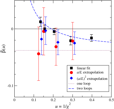
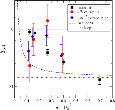
Figure 6: Beta function $\tilde{\beta}(u)$ of the SU(3)/adjoint theory (left) and the SU(4)/sextet theory (right), extrapolated to the continuum limit. Black squares and curves are the same as in Fig. 5. The points for the extrapolations have been displaced slightly for clarity.

Compared to Fig. 5, the linear extrapolations increase the error bars by a factor of 5, the quadratic extrapolations by only a factor of 3. The linear and quadratic extrapolations are mutually consistent for each data point; one can consider them separately as distinct models, or take their error bars together as a combination of statistical with systematic errors.

We note that the simple linear fits (6) typically give a large $\chi^{2}$ precisely because they neglect finite-lattice corrections. The extrapolations (8) and (9), on the other hand, are models aimed at removing the discretization error and indeed they result in acceptable $\chi^{2}$.

In the SU(3) theory, we can no longer tell whether the beta function crosses zero, and indeed the very shape of the function is not well determined. In the SU(4) theory, the extrapolations indicate a function that approaches zero and then veers off downwards.

IV Mass anomalous dimension

Following still the methods used in our previous work, we calculate the mass anomalous dimension from the scaling with $L$ of the pseudoscalar renormalization factor $Z_{P}$. The latter comes from the ratio

$$Z_{P}=\frac{c\sqrt{f_{1}}}{f_{P}(L/2)}.$$ (10)

$f_{P}$ is the propagator from a wall source at the $t=0$ boundary to a point pseudoscalar operator at time $L/2$. The normalization of the wall source is removed by the $\sqrt{f_{1}}$ factor, which comes from a boundary-to-boundary correlator. The constant $c$, which is an arbitrary normalization, is $1/\sqrt{2}$ in our convention.

We present in Tables 6 and 7 the values of $Z_{P}$ we find in the SU(3) and SU(4) theories, respectively; we plot them in Figs. 7 and 8.

Table 6: Pseudoscalar renormalization constant $Z_{P}$ measured in the SU(3)/adjoint theory.

$\beta$	$Z_{P}$
	$L=6a$	$L=8a$	$L=10a$	$L=12a$	$L=16a$
3.8	–	0.1333(4)	0.1243(5)	0.1169(3)	0.1070(7)
3.9	–	0.1418(4)	0.1306(4)	0.1222(3)	0.1119(6)
4.1	0.1760(4)	0.1550(5)	0.1426(4)	0.1352(6)	0.1225(8)
4.5	0.1990(4)	0.1775(6)	0.1656(5)	0.1546(3)	0.1427(8)
5.0	0.2193(4)	0.1998(8)	0.1881(7)	0.1788(5)	–

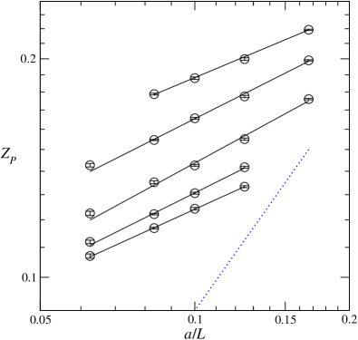
Figure 7: The pseudoscalar renormalization constant $Z_{P}$ vs. $L/a$ in the SU(3)/adjoint theory (Table 6). Top to bottom: $\beta=5.0,$ 4.5, 4.1, 3.9, 3.8. The straight lines are linear fits to each set of points at given $\beta$; the slope gives $\gamma_{m}$. The hypothetical dotted line corresponds to $\gamma_{m}=1$.

Table 7: Pseudoscalar renormalization constant $Z_{P}$ measured in the SU(4)/sextet theory.

$\beta$	$Z_{P}$
	$L=6a$	$L=8a$	$L=10a$	$L=12a$	$L=16a$
5.5	0.2149(10)	0.2022(11)	0.1906(12)	0.1801(7)	0.1681(14)
6.0	0.2311(9)	0.2150(9)	0.1995(8)	0.1918(12)	0.1747(13)
7.0	0.2558(6)	0.2376(6)	0.2243(6)	0.2123(8)	0.1981(11)
8.0	0.2820(4)	0.2616(6)	0.2496(5)	0.2374(5)	0.2242(8)
10.0	0.3201(3)	0.3037(4)	0.2929(4)	0.2844(4)	–

Figure 8: Same as Fig. 7, but for the SU(4)/sextet theory (Table 7). Top to bottom: $\beta=10.0,$ 8.0, 7.0, 6.0, 5.5.

As in the calculation of $\tilde{\beta}$, we begin with the simple fits, based on the slowness of the running of $1/g^{2}$ DeGrand:2011qd . Following the approximate scaling formula

$$Z_{P}(L)=Z_{P}(L_{0})\left(\frac{L_{0}}{L}\right)^{\gamma_{m}},$$ (11)

we fit the $Z_{P}$ data at each value of $\beta$ to

$$\log Z_{P}(L)=c_{0}+c_{1}\log\frac{8a}{L},$$ (12)

giving the straight lines plotted in the figures; the slope $c_{1}$ gives an estimate of $\gamma_{m}$. For an analysis of finite-volume effects, we drop successive volumes starting from the smallest, giving the sequence of $c_{1}^{(n)}$ as above. Again we extrapolate $c_{1}^{(n)}$ either linearly or quadratically to $a/L=0$. All these results are plotted in Fig. 9.

In both theories, the simple linear fits produce values of $\gamma_{m}$ that depart from the one-loop line and level off. In the SU(3) theory, the extrapolations drive the result downward. Overall, we have a bound $\gamma_{m}\lesssim 0.4$. In the SU(4) theory, the extrapolations are remarkably consistent with each other and with the original linear fit. $\gamma_{m}$ again agrees well with the one-loop line in weak coupling, and then deviates downward to level off below 0.3 for the linear fits, stretching to 0.35 for the extrapolations.

The behavior of $\gamma_{m}$ in both theories is remarkably similar to our what we found in the three 2ISR theories: SU(2)/triplet, SU(3)/sextet, and SU(4)/decuplet.

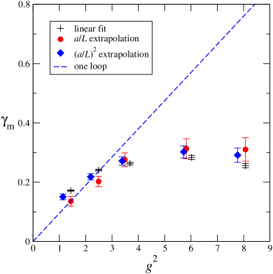
Figure 9: Mass anomalous dimension $\gamma_{m}(g^{2})$ of the SU(3)/adjoint theory (left) and the SU(4)/sextet theory (right), plotted as a function of $g^{2}(L=8a)$. Shown are the simple linear fits and the linear and quadratic extrapolations to the continuum limit. The points for the extrapolations have been displaced slightly where necessary. The brackets indicate the results of fits at $\beta=3.8$, which were obtained after dropping an outlying stream for $L=16a$; see Sec. II and Table 6. (Restoring the dropped stream to the averages moves the bracketed points upwards slightly: the simple linear fit by $1.4\sigma$, the linear extrapolation by $1.9\sigma$, and the quadratic extrapolation by $1.9\sigma$.)

V Conclusions

Our calculations reveal that the beta functions associated with the SF coupling in the two theories studied are small, everywhere smaller than the one-loop values. In the SU(4) theory, the running is even slower than what is expected in two loops. Our inability to disentangle possible lattice artifacts from real running prevents a more definite statement.

In all cases we have studied, the two in this paper and the 2ISR theories in our previous work, the mass anomalous dimension varies linearly with the SF gauge coupling when the coupling is small, and then levels off to a plateau at large gauge coupling. All the plateaus are at a level below 0.5.

Imagine now performing a lattice simulation for any of these systems at any value of the bare lattice coupling in which the system is in the same phase as at weak coupling. One will have access to physical scales ranging from the lattice spacing $a$ to the system size $L$, where (in the near future) $L/a$ will be smaller than about 100. The running coupling will scarcely evolve over this change of scale. Whether or not the system is actually at a fixed point, the slow evolution of the coupling implies that lattice spectroscopy will display systematics of scaling, broken by a nonzero fermion mass, by irrelevant operators, and by the effect of finite system volume. Given the size of the one-loop coefficient of the beta function, plus the observation that the running coupling in these theories always runs more slowly than one-loop expectations, this behavior is completely natural.

In all these lattice systems, typically one will encounter a confining phase with broken chiral symmetry when the bare coupling exceeds a certain value. Whether or not this describes continuum physics can in principle be decided by calculating the beta function as we have attempted, and determining whether an IRFP is encountered before chiral symmetry breaks. In the two systems studied in this paper, we were unable to resolve this question.

The great advantage of lattice QCD is that the bare coupling can be adjusted such that perturbation theory is valid at the lattice scale $a$, while at the same time the volume is big enough to accommodate even the lightest of the hadrons. The same is not true for nearly conformal theories. Whether the infrared physics is conformal or not, in order to probe it the bare coupling must be strong. One consequence is that the Symanzik effective action, defined around the gaussian fixed point, offers no guidance to the scaling dimensions of irrelevant operators. In a nearly conformal theory, where finite-lattice corrections are essentially functions of $a/L$, this also leaves us ignorant regarding the behavior of finite-volume corrections. Our extrapolations to infinite volume are then only models.

A comparison to the SF analysis of ordinary QCD (with small $N_{f}$ and triplet quarks) invites the question of why it is so difficult to produce good quality results for borderline-conformal theories. We believe that the answer lies in the fact that what is interesting is not the absolute uncertainty $\Delta\tilde{\beta}$ in the value of the beta function $\tilde{\beta}(g^{2})$; rather, it is the relative error, for which we take the ratio of the uncertainty to the one-loop constant value. The latter is proportional to the lowest order coefficient $b_{1}$. In QCD with three flavors, $b_{1}=9$; for the near-conformal theories, Table 1 lists values that are a good deal smaller. The QCD beta function is also increased by a positive $b_{2}$, whereas $b_{2}<0$ is a necessary feature of the borderline theories. Indeed, Table 1 shows that the SU(3)/adjoint theory studied here is a particularly difficult case to begin with.

The uncertainty $\Delta\tilde{\beta}$ scales with the ensemble size as $1/\sqrt{N}$, where $N$ is the number of uncorrelated measurements. The observable giving the SF coupling is essentially a surface quantity. It also includes data generated by a noisy estimator. Thus it has large inherent fluctuations as well as long-time autocorrelations underlying these fluctuations. While this is true for all theories, we found the SU(3)/adjoint model to be particularly intractable. New methods of computing running couplings will compete successfully with the SF if they can overcome these problems.

*

Appendix A

A.1 Choosing the value of $\beta^{\prime}$

To find an optimal value of $\beta^{\prime}$ for each theory, we do a series of short runs on small ($L=6a$) lattices to determine $\kappa_{c}(\beta)$ and then to measure the SF coupling $g^{2}$ along the $\kappa_{c}$ curve. For fixed $\beta^{\prime}$, $g^{2}$ grows as $\beta$ is decreased (see Figs. 10 and 11). Our aim is to reach the largest $g^{2}$ possible. This is limited by two effects that appear as $\beta$ is decreased: Either one reaches the point $\beta_{1}$ where the $\kappa_{c}(\beta)$ curve hits the first-order transition seen in Fig. 1, or the poor acceptance due to the increasing disorder makes simulation impractical. The encounter with the phase transition is indicated by vertical lines drawn for one value of $\beta^{\prime}$ in each of Figs. 10 and 11; for other values of $\beta^{\prime}$, we were stopped by acceptance so poor on these small lattices that simulation on larger lattices would have been impossible.

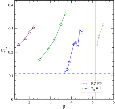
Figure 10: Inverse SF coupling versus gauge coupling $\beta$ for several choices of $\beta^{\prime}$ in the SU(3)/adjoint theory, measured with short runs on a $6^{4}$ lattice. The connected data sets are for (right to left) $\beta^{\prime}=-0.5$, 0, 0.5, 1.0. For $\beta^{\prime}=-0.5$, the vertical line marks the appearance of the first-order transition that makes $\kappa_{c}$ disappear for smaller $\beta$. The horizontal dashed line near the bottom of the graph marks the location of the Banks–Zaks (two-loop) fixed point. The horizontal dotted line marks where the one-loop $\gamma_{m}(g^{2})$ is equal to unity. Statistical error bars range from $\pm 0.01$ to $\pm 0.02$.

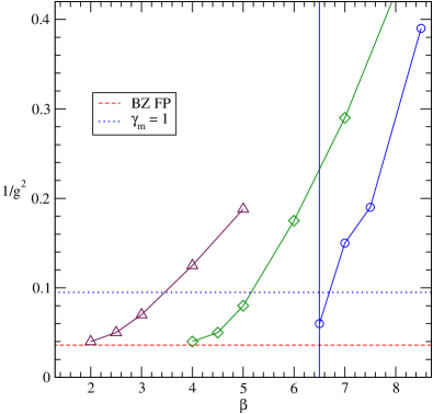
Figure 11: As in Fig. 10, but in the SU(4)/sextet theory. The connected data sets are for (right to left) $\beta^{\prime}=0$, 0.5, 1.0. The vertical line marks the appearance of the first-order transition for $\beta^{\prime}=0$.

For the SU(3)/adjoint theory we chose $\beta^{\prime}=0$ since it appeared to offer the largest range in $g^{2}$. As it turned out, longer runs on $6^{4}$ lattices showed that the three points plotted for the strongest couplings ($\beta=3.7$, 3.8, 3.9) in Fig. 10 represented metastable states, i.e., lying on the wrong side of the phase transition. We were nonetheless able to run at $\beta=3.8$ and 3.9 on larger lattices, as described in Sec. II. In the SU(4)/sextet theory no such issue arose; Fig. 11 shows why we chose $\beta^{\prime}=0.5$ for this theory.

Figures 10 and 11 may be compared to Fig. 1 in our paper on the SU(4)/decuplet theory DeGrand:2012qa . One may find there a demonstration of universality in weak coupling as $\beta^{\prime}$ is varied.

A.2 Continuum extrapolations

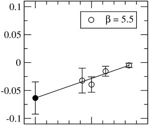
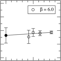
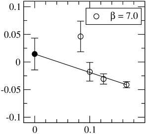
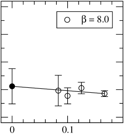
Figure 12: Successive fits $c_{1}^{(n)}$ giving the beta function $\tilde{\beta}$ of the SU(4)/sextet theory, as a function of $a/L_{n}$, where $L_{n}$ is the smallest lattice size used in the fit. The linear extrapolations to $a/L=0$ are shown.

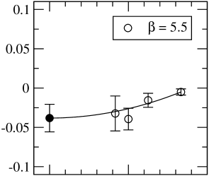
Figure 13: Same as Fig. 12, but showing the quadratic extrapolations to $a/L=0$.

To illustrate our method of continuum extrapolation, we show the values of $c_{1}^{(n)}$ for the beta function in the SU(4) theory in Figs. 12 and 13, along with their linear and quadratic extrapolations to $a/L=0$. The figures show the origin of the error bars in the extrapolated values at $L\to\infty$. The quadratic extrapolations result in smaller error bars because they have a longer lever arm between the smallest and largest lattices.

References

- (1) E. T. Neil, “Exploring Models for New Physics on the Lattice,” PoS LATTICE 2011, 009 (2011) [arXiv:1205.4706 [hep-lat]].
- (2) J. Giedt, “Lattice gauge theory and physics beyond the standard model,” PoS LATTICE 2012, 006 (2012).
- (3) B. Holdom, “Raising The Sideways Scale,” Phys. Rev. D 24, 1441 (1981).
- (4) K. Yamawaki, M. Bando and K. i. Matumoto, “Scale Invariant Technicolor Model And A Technidilaton,” Phys. Rev. Lett. 56, 1335 (1986).
- (5) C. T. Hill and E. H. Simmons, “Strong dynamics and electroweak symmetry breaking,” Phys. Rept. 381, 235 (2003) [Erratum-ibid. 390, 553 (2004)] [arXiv:hep-ph/0203079];
- (6) F. Sannino and K. Tuominen, “Orientifold theory dynamics and symmetry breaking,” Phys. Rev. D 71, 051901 (2005) [arXiv:hep-ph/0405209].
- (7) D. K. Hong, S. D. H. Hsu and F. Sannino, “Composite Higgs from higher representations,” Phys. Lett. B 597, 89 (2004) [arXiv:hep-ph/0406200].
- (8) D. D. Dietrich and F. Sannino, “Conformal window of SU() gauge theories with fermions in higher dimensional representations,” Phys. Rev. D 75, 085018 (2007) [hep-ph/0611341].
- (9) W. E. Caswell, “Asymptotic behavior of nonabelian gauge theories to two loop order,” Phys. Rev. Lett. 33, 244 (1974).
- (10) T. Banks and A. Zaks, “On the phase structure of vector-like gauge theories with massless fermions,” Nucl. Phys. B 196, 189 (1982).
- (11) T. Appelquist, K. D. Lane and U. Mahanta, “On The Ladder Approximation For Spontaneous Chiral Symmetry Breaking,” Phys. Rev. Lett. 61, 1553 (1988).
- (12) A. G. Cohen, and H. Georgi, “Walking Beyond The Rainbow,” Nucl. Phys. B 314, 7 (1989).
- (13) M. Lüscher, R. Narayanan, P. Weisz and U. Wolff, “The Schrödinger functional: A Renormalizable probe for non-Abelian gauge theories,” Nucl. Phys. B 384, 168 (1992) [arXiv:hep-lat/9207009].
- (14) M. Lüscher, R. Sommer, P. Weisz and U. Wolff, “A precise determination of the running coupling in the SU(3) Yang-Mills theory,” Nucl. Phys. B 413, 481 (1994) [arXiv:hep-lat/9309005].
- (15) S. Sint, “On the Schrödinger functional in QCD,” Nucl. Phys. B 421, 135 (1994) [arXiv:hep-lat/9312079]; “One Loop Renormalization Of The QCD Schrödinger Functional,” 451, 416 (1995) [arXiv:hep-lat/9504005].
- (16) S. Sint and R. Sommer, “The running coupling from the QCD Schrödinger functional: A one loop analysis,” Nucl. Phys. B 465, 71 (1996) [arXiv:hep-lat/9508012].
- (17) K. Jansen and R. Sommer [ALPHA collaboration], “O() improvement of lattice QCD with two flavors of Wilson quarks,” Nucl. Phys. B 530, 185 (1998) [Erratum-ibid. B 643, 517 (2002)] [arXiv:hep-lat/9803017].
- (18) M. Della Morte et al. [ALPHA Collaboration], “Computation of the strong coupling in QCD with two dynamical flavours,” Nucl. Phys. B 713, 378 (2005) [arXiv:hep-lat/0411025].
- (19) T. DeGrand, Y. Shamir, B. Svetitsky, “Infrared fixed point in SU(2) gauge theory with adjoint fermions,” Phys. Rev. D83, 074507 (2011). [arXiv:1102.2843 [hep-lat]].
- (20) Y. Shamir, B. Svetitsky and T. DeGrand, “Zero of the discrete beta function in SU(3) lattice gauge theory with color sextet fermions,” Phys. Rev. D 78, 031502 (2008) [arXiv:0803.1707 [hep-lat]].
- (21) T. DeGrand, Y. Shamir, B. Svetitsky, “Running coupling and mass anomalous dimension of SU(3) gauge theory with two flavors of symmetric-representation fermions,” Phys. Rev. D82, 054503 (2010). [arXiv:1006.0707 [hep-lat]].
- (22) T. DeGrand, Y. Shamir and B. Svetitsky, “Mass anomalous dimension in sextet QCD,” Phys. Rev. D 87, 074507 (2013) [arXiv:1201.0935 [hep-lat]].
- (23) T. DeGrand, Y. Shamir and B. Svetitsky, “SU(4) lattice gauge theory with decuplet fermions: Schrödinger functional analysis,” Phys. Rev. D 85, 074506 (2012) [arXiv:1202.2675 [hep-lat]].
- (24) T. Appelquist, G. T. Fleming and E. T. Neil, “Lattice study of the conformal window in QCD-like theories,” Phys. Rev. Lett. 100, 171607 (2008) [Erratum-ibid. 102, 149902 (2009)] [arXiv:0712.0609 [hep-ph]].
- (25) T. Appelquist, G. T. Fleming and E. T. Neil, “Lattice Study of Conformal Behavior in SU(3) Yang-Mills Theories,” Phys. Rev. D 79, 076010 (2009) [arXiv:0901.3766 [hep-ph]].
- (26) A. J. Hietanen, K. Rummukainen and K. Tuominen, “Evolution of the coupling constant in SU(2) lattice gauge theory with two adjoint fermions,” Phys. Rev. D 80, 094504 (2009) [arXiv:0904.0864 [hep-lat]].
- (27) F. Bursa, L. Del Debbio, L. Keegan, C. Pica and T. Pickup, “Mass anomalous dimension in SU(2) with two adjoint fermions,” Phys. Rev. D 81, 014505 (2010) [arXiv:0910.4535 [hep-ph]].
- (28) F. Bursa, L. Del Debbio, L. Keegan, C. Pica and T. Pickup, “Mass anomalous dimension in SU(2) with six fundamental fermions,” Phys. Lett. B 696, 374 (2011) [arXiv:1007.3067 [hep-ph]].
- (29) M. Hayakawa, K. -I. Ishikawa, Y. Osaki, S. Takeda, S. Uno and N. Yamada, “Running coupling constant of ten-flavor QCD with the Schrödinger functional method,” Phys. Rev. D 83, 074509 (2011) [arXiv:1011.2577 [hep-lat]].
- (30) T. Karavirta, J. Rantaharju, K. Rummukainen and K. Tuominen, “Determining the conformal window: SU(2) gauge theory with , 6 and 10 fermion flavours,” JHEP 1205, 003 (2012) [arXiv:1111.4104 [hep-lat]].
- (31) M. Hayakawa, K. -I. Ishikawa, Y. Osaki, S. Takeda and N. Yamada, “Lattice study on two-color QCD with six flavors of dynamical quarks,” PoS LATTICE 2012, 040 (2012) [arXiv:1210.4985 [hep-lat]].
- (32) G. Voronov, “Two-Color Schrödinger Functional with Six Flavors of Stout-Smeared Wilson Fermions,” PoS LATTICE 2012, 039 (2012) [arXiv:1212.1376 [hep-lat]].
- (33) J. Rantaharju, K. Rummukainen and K. Tuominen, “Running coupling in SU(2) with adjoint fermions,” arXiv:1301.2373 [hep-lat].
- (34) S. Sint and P. Weisz [ALPHA collaboration], “The running quark mass in the SF scheme and its two-loop anomalous dimension,” Nucl. Phys. B 545, 529 (1999) [arXiv:hep-lat/9808013].
- (35) S. Capitani, M. Lüscher, R. Sommer and H. Wittig [ALPHA Collaboration], “Non-perturbative quark mass renormalization in quenched lattice QCD,” Nucl. Phys. B 544, 669 (1999) [arXiv:hep-lat/9810063].
- (36) M. Della Morte et al. [ALPHA Collaboration], “Non-perturbative quark mass renormalization in two-flavor QCD,” Nucl. Phys. B 729, 117 (2005) [arXiv:hep-lat/0507035].
- (37) J. B. Kogut, J. Shigemitsu and D. K. Sinclair, “Chiral Symmetry Breaking With Octet And Sextet Quarks,” Phys. Lett. B 145, 239 (1984).
- (38) E. Gerstenmayer, M. Faber, W. Feilmair, H. Markum and M. Müller, “Quark Confinement With Dynamical Fermions In Higher Representations,” Phys. Lett. B 231, 453 (1989).
- (39) F. Karsch and M. Lütgemeier, “Deconfinement and chiral symmetry restoration in an SU(3) gauge theory with adjoint fermions,” Nucl. Phys. B 550, 449 (1999) [hep-lat/9812023].
- (40) M. E. Peskin, “The Alignment of the Vacuum in Theories of Technicolor,” Nucl. Phys. B 175, 197 (1980).
- (41) F. Basile, A. Pelissetto and E. Vicari, “The Finite-temperature chiral transition in QCD with adjoint fermions,” JHEP 0502, 044 (2005) [hep-th/0412026].
- (42) J. Engels, S. Holtmann and T. Schulze, “Scaling and Goldstone effects in a QCD with two flavors of adjoint quarks,” Nucl. Phys. B 724, 357 (2005) [hep-lat/0505008].
- (43) G. Cossu, M. D’Elia, A. Di Giacomo, G. Lacagnina and C. Pica, “Monopole condensation in two-flavor adjoint QCD,” Phys. Rev. D 77, 074506 (2008) [arXiv:0802.1795 [hep-lat]].
- (44) M. Unsal, “Magnetic bion condensation: A new mechanism of confinement and mass gap in four dimensions,” Phys. Rev. D 80, 065001 (2009) [arXiv:0709.3269 [hep-th]].
- (45) G. Cossu and M. D’Elia, “Finite size phase transitions in QCD with adjoint fermions,” JHEP 0907, 048 (2009) [arXiv:0904.1353 [hep-lat]].
- (46) A. Deuzeman, M. P. Lombardo and E. Pallante, “The Physics of eight flavours,” Phys. Lett. B 670, 41 (2008) [arXiv:0804.2905 [hep-lat]].
- (47) K. Miura, M. P. Lombardo and E. Pallante, “Chiral phase transition at finite temperature and conformal dynamics in large QCD,” Phys. Lett. B 710, 676 (2012) [arXiv:1110.3152 [hep-lat]].
- (48) A. Cheng, A. Hasenfratz and D. Schaich, “Novel phase in SU(3) lattice gauge theory with 12 light fermions,” Phys. Rev. D 85, 094509 (2012) [arXiv:1111.2317 [hep-lat]].
- (49) A. Deuzeman, M. P. Lombardo, T. Nunes Da Silva and E. Pallante, “The bulk transition of QCD with twelve flavors and the role of improvement,” Phys. Lett. B 720, 358 (2013) [arXiv:1209.5720 [hep-lat]].
- (50) K. Miura and M. P. Lombardo, “Lattice Monte-Carlo study of pre-conformal dynamics in strongly flavoured QCD in the light of the chiral phase transition at finite temperature,” Nuclear Physics B 871, 52 (2013) [arXiv:1212.0955 [hep-lat]].
- (51) J. B. Kogut and D. K. Sinclair, “Thermodynamics of lattice QCD with 2 flavours of colour-sextet quarks: A model of walking/conformal Technicolor,” Phys. Rev. D 81, 114507 (2010) [arXiv:1002.2988 [hep-lat]].
- (52) J. B. Kogut and D. K. Sinclair, “Thermodynamics of lattice QCD with 2 sextet quarks on =8 lattices,” Phys. Rev. D 84, 074504 (2011) [arXiv:1105.3749 [hep-lat]].
- (53) J. B. Kogut and D. K. Sinclair, “Thermodynamics of lattice QCD with 3 flavours of colour-sextet quarks,” Phys. Rev. D 85, 054505 (2012) [arXiv:1111.3353 [hep-lat]].
- (54) D. K. Sinclair and J. B. Kogut, “QCD with colour-sextet quarks,” PoS LATTICE 2012, 026 (2012) [arXiv:1211.0712 [hep-lat]].
- (55) T. DeGrand, Y. Shamir and B. Svetitsky, “Phase structure of SU(3) gauge theory with two flavors of symmetric-representation fermions,” Phys. Rev. D 79, 034501 (2009) [arXiv:0812.1427 [hep-lat]].
- (56) B. Sheikholeslami and R. Wohlert, “Improved continuum limit lattice action for QCD with Wilson fermions,” Nucl. Phys. B 259, 572 (1985).
- (57) Y. Shamir, B. Svetitsky, and E. Yurkovsky, “Improvement via hypercubic smearing in triplet and sextet QCD,” Phys. Rev. D83, 097502 (2011). [arXiv:1012.2819 [hep-lat]].
- (58) A. Hasenfratz and F. Knechtli, “Flavor symmetry and the static potential with hypercubic blocking,” Phys. Rev. D 64, 034504 (2001) [arXiv:hep-lat/0103029].
- (59) A. Hasenfratz, R. Hoffmann and S. Schaefer, “Hypercubic smeared links for dynamical fermions,” JHEP 0705, 029 (2007) [arXiv:hep-lat/0702028].
- (60) Y. Iwasaki, K. Kanaya, S. Sakai and T. Yoshié, “Quark confinement and number of flavors in strong coupling lattice QCD,” Phys. Rev. Lett. 69, 21 (1992).
- (61) Y. Iwasaki, K. Kanaya, S. Kaya, S. Sakai and T. Yoshié, “Phase structure of lattice QCD for general number of flavors,” Phys. Rev. D 69, 014507 (2004) [arXiv:hep-lat/0309159].
- (62) K. Nagai, G. Carrillo-Ruiz, G. Koleva and R. Lewis, “Exploration of SU() gauge theory with many Wilson fermions at strong coupling,” Phys. Rev. D 80, 074508 (2009) [arXiv:0908.0166 [hep-lat]].
- (63) B. Svetitsky, Y. Shamir and T. DeGrand, “Sextet QCD: slow running and the mass anomalous dimension,” PoS LATTICE 2010, 072 (2010) [arXiv:1010.3396 [hep-lat]].
- (64) B. Svetitsky, “Conformal or confining—results from lattice gauge theory for higher-representation gauge theories,” PoS ConfinementX 271 (2013) [arXiv:1301.1877 [hep-lat]].
- (65) M. Hasenbusch, “Speeding up the Hybrid-Monte-Carlo algorithm for dynamical fermions,” Phys. Lett. B 519, 177 (2001) [arXiv:hep-lat/0107019].
- (66) C. Urbach, K. Jansen, A. Shindler and U. Wenger, “HMC algorithm with multiple time scale integration and mass preconditioning,” Comput. Phys. Commun. 174, 87 (2006) [arXiv:hep-lat/0506011].
- (67) T. Takaishi and P. de Forcrand, “Testing and tuning new symplectic integrators for hybrid Monte Carlo algorithm in lattice QCD,” Phys. Rev. E 73, 036706 (2006) [arXiv:hep-lat/0505020].
- (68) http://www.physics.utah.edu/detar/milc/