Computation of the thermal conductivity using classical and quantum molecular dynamics based methods.

Abstract

The thermal conductivity of a model for solid argon is investigated using nonequilibrium molecular dynamics methods, as well as the traditional Boltzmann transport equation approach with input from molecular dynamics calculations, both with classical and quantum thermostats. A surprising result is that, at low temperatures, only the classical molecular dynamics technique is in agreement with the experimental data. We argue that this agreement is due to a compensation of errors, and raise the issue of an appropriate method for calculating thermal conductivities at low (below Debye) temperatures.

I Introduction

Different methods are available for calculating thermal conductivities of crystalline solids. Stackhouse and Stixrude (2010) The most standard approach involves a calculation of the phonon properties of the system, which are connected to the thermal conductivity through the Boltzmann transport equation. Alternative methods are based on equilibrium molecular dynamics (MD) and non-equilibrium molecular dynamics (NEMD). Jund and Jullien (1999a); Müller-Plathe (1997); Stackhouse and Stixrude (2010)

The methods based on MD or NEMD are restricted to the classical limit, i.e. the limit of high temperatures. In standard MD, nuclear degrees of freedom are treated classically and quantum effects such as zero-point vibrations are not accounted for. In order to incorporate quantum effects, corrections to the thermal conductivity, based on a rescaling of the heat capacity, are commonly applied. These kind of corrections, however, are not generally accepted as reliable. Turney et al. Turney et al. (2009a) discussed their validity, and showed that this approach is oversimplified and is not generally applicable, while other authors have found an improvement of the classical thermal conductivity by applying such corrections. Li et al. (1998); Jund and Jullien (1999b) Quantum effects, on the other hand, are assumed negligible depending on the capability of the classical description to describe the thermal conductivity, but independently of its limitations for predicting heat capacities or phonon lifetimes, properties directly related with the thermal conductivity. A common example is the case of solid argon. In spite of the limitations of the classical theory to predict correctly the heat capacity, a reliable description of the thermal conductivity, at temperatures well below the Debye value, is obtained from classical molecular dynamics. Kaburaki et al. (2007); McGaughey and Kaviany (2004a)

Quantum effects on the thermal conductivity can be obtained from anharmonic lattice dynamics, by using the Boltzmann transport equation. Srivastava (1990) This methodology, nonetheless, results in much more expensive computations than molecular dynamics. It requires the full calculation of the vibrational spectrum of the system, as well as the third derivatives of the energy, something unmanageable for large or aperiodic systems. Moreover, the Boltzmann transport calculation relies on approximate theoretical expressions for the phonon lifetime and for the conductivity itself, as opposed to the MD and NEMD formalisms that are in principle exact.

Recently, a Langevin type thermostat with a coloured noise was proposed  Dammak et al. (2009); Ceriotti et al. (2009) and implemented Barrat and Rodney (2011) by different authors in order to incorporate quantum effects in molecular dynamics. The quantum thermostat allows to recover the correct average quantum energy of a system by coupling every degree of freedom to a fictitious quantum bath, in such a way that a harmonic oscillator acquires an energy given by the Bose-Einstein distribution. As such the method is expected to provide a good description of solids in the harmonic limit, and has been shown to also work well for low temperature liquids, in terms of static properties. Dammak et al. (2009) At high temperatures, the quantum thermostat reduces to a standard Langevin thermostat. This semi-classical approach offers the possibility of performing direct thermal conductivity calculations, by using molecular dynamics, independent of the temperature regime. Savin et al. Savin et al. (2012) have applied this methodology to the study of heat transport in low-dimensional nanostructures from non-equilibrium molecular dynamics (NEMD). In the case of a NEMD simulation there are regions of the system free of thermostat, and one will have to check the validity of the quantum thermostat under such conditions. Moreover, the quantum thermostat is not an exact representation of the quantum behavior, and for anharmonic systems suffers from “zero-point energy leakage” (see Ref. Ceriotti et al., 2009 and section III below). It is unknown if this influences thermal transport properties. Here we present an overview of the advances and challenges for using such kind of thermostats to address thermal transport studies at low temperatures (below the Debye temperature $T_{\text{D}}$). In our study we use different MD based methods for calculating the thermal conductivity of solid argon, a simple system that is well described in the literature and, as pointed out before, is particularly well described by classical MD.

The paper is organized as follows. In Sec. II we present the various methods used for estimating the thermal conductivity. In Sec. III we briefly introduce the quantum thermostat, we discuss about the zero-point energy leakage problem and its reliability for working under equilibrium and non-equilibrium conditions. In the last section we present and discuss our results for the thermal conductivity of solid Argon.

II Methodology

The standard methods to compute thermal conductivities are based either on molecular dynamics or lattice dynamics, or a combination of both. In this work, we used non-equilibrium molecular dynamics (NEMD) Jund and Jullien (1999a); Müller-Plathe (1997); Stackhouse and Stixrude (2010) and Boltzmann transport equation molecular dynamics (BTE-MD). Turney et al. (2009b); McGaughey and Kaviany (2004b) We did not use Green-Kubo based methods, Green (1954); Kubo (1957) which have smaller size effects than NEMD, because the quantum thermostat is not compatible with this approach (see discussion below). However, the cells employed here are large enough to avoid any strong size effects in NEMD.

In NEMD, the periodic simulation cell is divided into $N$ slabs, and a temperature gradient is imposed by coupling two selected slabs to two thermostats at different temperatures, $T_{\text{1}}$ and $T_{\text{2}}$ with $T_{\text{1}}<T_{\text{2}}$. In a periodic system, the thermostated slabs are separated by a distance equal to one half of the simulation cell length. The remaining slabs are not thermostated. The system is then allowed to reach a steady state, where on average the energy creation rate of the thermostat at $T_{\text{2}}$ is equal to the energy removal rate of the thermostat at $T_{\text{1}}$. Calculating the heat flux $j_{i}$ required to maintain the gradient of temperature ${\nabla}_{j}T$ from the heat power of the source and the sink, one can estimate the thermal conductivity from Fourier’s law:

$$j_{i}=-\kappa_{ij}\,{\nabla}_{j}\,T.$$ (1)

In this work we assumed materials of isotopic symmetry. The thermal conductivity is then a scalar, and the temperature gradient and heat flux are parallel.

Equation (1) can alternatively be implemented by imposing the heat flux $\vec{J}$ and calculating the resulting temperature gradient. A common approach in this case, Jund and Jullien (1999a); Müller-Plathe (1997) is to rescale the velocities, $\vec{v}_{\text{h}}$, of the atoms in the hot region according to

$$\vec{v}_{\text{h}}\,^{\prime}=\vec{v}_{\text{G}}+\alpha(\vec{v}_{\text{h}}-\vec{v}_{\text{G}}),$$ (2)

where $\vec{v}_{\text{G}}$ is the velocity of the center of mass of the region, and

$$\alpha=\sqrt{1+\frac{\Delta\,\epsilon}{k_{\text{R}}}}.$$ (3)

Here $\Delta\,\epsilon$ is the amount of heat transferred through the system, and $k_{\text{R}}$ is the relative kinetic energy given by

$$k_{\text{R}}=\frac{1}{2}\sum_{i\in\text{hot}}m_{i}\;\vec{v}_{i}^{\;2}-\frac{1}{2}\sum_{i\in\text{hot}}m_{i}\;\vec{v}_{\text{G}}^{\;2}.$$ (4)

In this manner, a constant heat flux

$$J=\frac{\Delta\,\epsilon}{2\,A\,\Delta\,t}$$ (5)

is imposed, where $A$ is the cross sectional area of the simulation cell perpendicular to the heat flow, and $\Delta t$ is the time step. We implemented both NEMD methods and checked that they are fully consistent with one another. In the following, we will not distinguish between them and will simply refer to them as the NEMD approach.

An alternative expression for the thermal conductivity of an isotropic material reads Srivastava (1990); Turney et al. (2009b)

$$\kappa=\sum_{\vec{q}}\sum_{\nu}^{3\,(N-1)}C_{\text{ph}}(\vec{q},\nu)\,{v}_{\text{g}}^{\,2}(\vec{q},\nu)\,\tau(\vec{q},\nu),$$ (6)

where $C_{\text{ph}}$ is the volumetric phonon specific heat, $\vec{v}_{\text{g}}$ is the phonon group velocity and $\tau$ the phonon lifetime. The sum runs over all wave vectors, $\vec{q}$, within the Brillouin zone of the periodic structure, and over the $3\,N$ polarization indices, where $N$ is the number of atoms in the elementary cell under consideration, so that contributions from all normal modes of the system are considered. In Eq. (6), the specific heats and group velocities can be computed using lattice dynamics, while the phonon lifetimes can be obtained using either lattice dynamics or a combination of lattice dynamics and molecular dynamics. Turney et al. (2009b); Srivastava (1990) In the following, we will use only the latter approach, referred to as the BTE-MD method.

Group velocities are obtained by evaluating the derivative of the dispersion curves, $\omega(q)$, over a set of 6 $q$-points within a radius 0.0001 $\AA^{-1}$ around the $\Gamma$ point. Phonon frequencies and specific heats are calculated at the $\Gamma$ point, in supercells that contain from 256 to 4000 atoms.

Phonon lifetimes are obtained from the energy autocorrelation function of each normal mode

$$E^{\,\vec{q},\nu}(t) = \frac{Q^{\ast}(\vec{q},\nu)\,Q(\vec{q},\nu)}{2}\,+$$

$$\frac{\omega^{\,2}\,(\vec{q},\nu)\;\dot{Q}^{\ast}(\vec{q},\nu)\,\dot{Q}(\vec{q},\nu)}{2},$$

with

$$Q(\,\vec{q},\nu) = \sum_{j=1}^{N}\,\left[\frac{m_{j}}{N}\right]^{1/2}\text{exp}[{-i\vec{q}\cdot\vec{r}_{j,0}}]\,\times$$

$$\,\vec{e}\,(\vec{q},\nu)\cdot[\vec{r}_{j}-\vec{r}_{j,0}]$$

the time-dependent normal mode coordinate. The eigenvectors $\vec{e}({\,\vec{q},\nu})$ are obtained from lattice dynamics, and the relative displacement, $\vec{r}_{j}-\vec{r}_{j,0}$, of atom $j$, is sampled using molecular dynamics. The phonon lifetimes $\tau$ are then obtained by fitting the following relation

$$e^{-t/\tau(\,\vec{q},\nu)}=\frac{\langle E^{\,\vec{q},\nu}(t)\,E^{\,\vec{q},\nu}(0)\rangle}{\langle E^{\,\vec{q},\nu}(0)\,E^{\,\vec{q},\nu}(0)\rangle}.$$ (9)

III Quantum thermostat

III.1 Overview

The key idea behind the quantum thermostat is to adjust to the manner in which energy is distributed among the normal modes of a harmonic system. In the classical limit, the equipartition theorem is fulfilled and all modes have the same energy, while in the quantum regime, the energy of each mode is distributed according to Bose-Einstein statistics. The quantum Langevin thermostat enforces this distribution by using a frequency-dependent noise function (coloured noise).

As in the classical approach using a Langevin thermostat, each particle is coupled to a fictitious bath by including in the equations of motion a random force and a dissipation term related by the fluctuation-dissipation theorem. Risken (1989) Accordingly, the equation of motion of a degree of freedom $x$, of a particle of mass $m$, in presence of an external force $F(x)$, becomes

$$m\,\ddot{x}=-\gamma\,m\;\dot{x}+F(x)+{\sqrt{2\,m\,\gamma}\,\Theta(t)},$$ (10)

where $\Theta(t)$ is a coloured noise with a power spectral density (PSD) given by the Bose-Einstein distribution

$$\tilde{\Theta}(\omega) = \int e^{-i\omega\,t}\langle\,\Theta(t)\,\Theta(t^{\prime})\,\rangle d\,t$$

$$= \hbar\,|\omega|\left(\frac{1}{2}+\frac{1}{e^{\,\hbar\,|\,\omega\,|\,k_{\text{B}}\,T}-1}\right),$$

including the zero point energy. The classical regime is recovered at high temperature, where the above PSD becomes independent of the frequency and equals $k_{\text{B}}\,T$. Grest et al. (1986) We also note here that the use of a Langevin equation implies the absence of local energy conservation; hence a Green-Kubo approach, based on the notion that local energy fluctuations undergo a diffusive motion, is not appropriate in a system that is coupled to a local (quantum or classical) heat bath.

In practice, $\tilde{\Theta}(\omega)$ is generated by using a signal processing method based on filtering a white noise. Oppenheim and Schafer (1999) A filter

$$\tilde{H}(\omega)=\sqrt{\tilde{\Theta}(\omega)}$$ (12)

with Fourier transform $H(t)$ is introduced, and $\Theta(t)$ is obtained by convoluting $H(t)$ with a random white noise, $r(t)$, of power spectral density $\tilde{R}(\omega)$=1, such that

$$\Theta(t)=\int\limits_{-\infty}^{\infty}H(s)\,r(t-s)\,ds.$$ (13)

Thus, the power spectral density of the resulting noise is

$$\left|\tilde{H}(\omega)\right|^{2}\tilde{R}(\omega)=\tilde{\Theta}(\omega),$$ (14)

which satisfies Eq. ​(III.1). The method is simple and can be easily implemented in a discrete molecular dynamics algorithm. From a computational point of view, the quantum thermostat does not slow down the calculations, the only difference with a classical thermostat being the convolution operation in Eq. ​(13). In terms of memory, the quantum thermostat is more demanding because it requires to store a finite number of past values of the white noise and of the filter in order to compute Eq. ​(13). However, the memory requirement for the thermostat scales linearly with the system size and is easily manageable with current computers. Moreover, it avoids generating and storing the entire time-series of random numbers as done in other implementations of the quantum thermal bath. Dammak et al. (2009) Further details concerning the method are given in Ref. Barrat and Rodney, 2011.

III.2 Zero-point energy leakage

By coupling a system to the quantum thermostat, each harmonic mode can in principle be equilibrated at the correct quantum harmonic energy given by Eq. (III.1). However, as the equations that are solved describe classical coordinates, the zero point energy in these equations corresponds to the finite amplitude vibration of a classical coordinate. As such this zero point energy can be exchanged between modes, in contrast with a true quantum zero point energy.

Such an exchange becomes possible when an anharmonic coupling between the modes is introduced, and leads to the phenomenon of ”zero-point energy leakage” (ZPE), where the zero point energy is transferred from the high-energy modes to low-energy modes, so as to homogenize the energy among the modes. Miller et al. (1989); Alimi et al. (1992); Ben-Nun and Levine (1996); Habershon and Manolopoulos (2009); Czakó et al. (2010) As the thermostat cannot fully counterbalance the leakage, an equilibrium is reached where the energy per mode is neither constant, nor as inhomogeneous as in Bose-Einstein distribution. An example is shown in Fig. 1 (left panel) in the case of a perfect crystal of aluminum at 10 K modeled with a Lennard-Jones potential. A coloured noise with power spectral density $\tilde{\Theta}_{A}(\omega)=\tilde{\Theta}(\omega)$ directly from Eq. (III.1) was used and results in an excess of energy in modes with frequency less than about 40 THz and a deficiency in energy for modes above that value.

One way to correct for the leakage is to modify the power spectral density of the filter, such that after equilibration of the leakage, the system reaches an energy-mode distribution which follows the Bose-Einstein distribution. An example is shown in Fig. 1 (right panel) with the adjusted power spectral density, $\tilde{\Theta}_{B}(\omega)$, shown as a dotted line. The resulting energy distribution (asterisks) is in much better agreement with the desired Bose-Einstein distribution (full line) than the one obtained using the original filter, shown in the left panel. The leakage is however not perfectly corrected, as can be seen from the Fourier transform of the velocity auto-correlation function (VAF) shown in Fig. 1 (bottom panel). Bear in mind that in classical MD, i.e. when a thermostat fulfilling the equipartition theorem of energy is used, the Fourier transform of the VAF equals the phonon density of states (DOS) times $k_{\text{B}}\,T/m$; in the quantum case, we obtain the phonon DOS times the phonon population function [Eq. (III.1)]. Figure 1 compares results obtained with the two coloured noises, $\tilde{\Theta}_{A}(\omega)$ and $\tilde{\Theta}_{B}(\omega)$, to the exact distribution. The latter is estimated by calculating the vibrational DOS, using a classical thermal bath (CTB), multiplied by $\tilde{\Theta}(\omega)$. In the case where $\tilde{\Theta}_{A}(\omega)=\tilde{\Theta}(\omega)$ (dashed blue line), the ZPE leakage results in an underpopulation of the high-energy modes ($\omega>45$ THz) and an overpopulation of the low-energy modes. The corrected coloured noise $\tilde{\Theta}_{B}(\omega)$ (green dotted line) yields a much better, although not perfect, agreement with the exact distribution, but fitting such power spectral density is technically difficult. The corrected PSD is both system- and temperature-dependent, making the direct application of this procedure rather tedious.

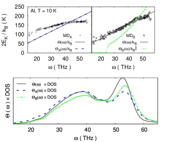
Figure 1: Scaled kinetic energy distribution per mode obtained from MD simulations. Left top panel: values obtained using a noise with power spectral density $\tilde{\Theta}_{A}(\omega)$ equal to the Bose-Einstein distribution $\tilde{\Theta}(\omega)$ [Eq. (III.1)]. Right top panel: values obtained using a noise with power spectral density $\tilde{\Theta}_{B}(\omega)$. Bottom panel: vibrational phonon spectrum times the phonon density of state. The full gray line was obtained by calculating the DOS using a classical thermal bath and multiplying by $\tilde{\Theta}(\omega)$. The other data were obtained directly from the Fourier transform of the velocity auto-correlation function (VAF). Calculations were performed for solid aluminum at 10 K using a Lennard-Jones potential.

In spite of the zero point energy leakage, quantum Langevin thermostats have been successfully used to map out the diamond-graphite coexistence curve, Ceriotti et al. (2009) as well as the proton momentum distribution in hydrogen-storage materials. Ceriotti et al. (2010) The quantum effects accounted for the thermostat were relevant, in these cases, for a correct description of the systems. Expecting the same degree of accuracy of the method for describing thermal conductivity properties, our calculations were performed omitting any correction concerning the leakage. However, as will be shown later, this introduces a serious limitation for the method.

III.3 Quantum thermostat and NEMD

Despite the zero-point energy leakage described above, the quantum thermostat allows to recover the correct temperature dependence of the equilibrium average thermal energy and heat capacity. Figure 2 shows an example in the case of solid argon. Here every degree of freedom of the system is coupled to the thermostat.

In the present semi-classical approach, we should distinguish between the temperature used as input of the thermostat, which is the true (quantum) temperature of the system, denoted as $T$, and the temperature measured from the kinetic energy of the system, which we call the classical temperature, $T^{\text{C}}$. The relation between both, in the case of solid argon, is shown in Fig. 2. In the harmonic approximation, we have:

$$T^{\text{C}}=\frac{1}{3(N-1)k_{\text{B}}}\sum\limits_{i}^{3(N-1)}\hbar\,\omega_{i}\,\left(\frac{1}{2}+\frac{1}{e^{\,\hbar\,\,\omega_{i}\,/\,k_{\text{B}}\,T}-1}\right).$$ (15)

At high temperature, the quantum temperature converges toward the classical value. When $T$ decreases to zero, $T^{\text{C}}$ converges to the zero-point energy of the system (expressed in Kelvins).

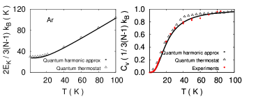
Figure 2: Left panel: Scaled average kinetic energy per degree of freedom, i.e. by definition the classical temperature, $T^{\text{C}}$, as a function of temperature. Right panel: Specific heat as a function of temperature obtained from molecular dynamics compared to experimental data Klein et al. (1969) and the quantum harmonic approximation. Within the harmonic approximation we have $C_{\text{v}}=\frac{\,\,\,\,d\,T^{\text{C}}}{d\,T}$, see Eq. 15. The phonon spectrum was obtained from lattice dynamics calculations performed at the $\Gamma$-point, using a 1280-atoms cell.

In NEMD, part of the system is not thermostated, and will not be directly coupled to a quantum thermal bath. It is not straightforward if the interaction between thermalized and non-thermalized parts will transfer the frequency-dependent energy. In order to explore the evolution of the system under such conditions, we performed a test simulation with the same configuration as NEMD, but coupling both thermostated slabs to quantum thermostats at the same temperature. Figure 3 shows the instantaneous kinetic energy and the Fourier transform of the VAF, once the system has reached equilibrium. Averages were performed over atoms in different regions of the cell, either thermostated or not. As can be seen, the thermostat-free regions (left panel, dashed line) have reached an average temperature in agreement with the one imposed in the thermostated regions (full red line). The larger fluctuations in the thermostated regions are due to the fact that averages are computed over smaller numbers of atoms. Moreover, the Fourier transform of the VAF shown in Fig. (3) (right panel) shows that the same frequency-dependent energy distribution is obtained in both regions, proving that a system can be equilibrated with a mode-dependent energy by applying a quantum thermostat only to a subset of the system. It should be pointed out, however, that the thermostated regions must have a size comparable or greater than the one of the ”free” regions. If this is not the case, the thermostated regions are not sufficient to thermostat the free part, which tends to relax towards a classical energy distribution. This is in contrast with the classical case, in which the thermostating of a few degrees of freedom is, in principle, sufficient to impose the temperature in an arbitrarily large system.

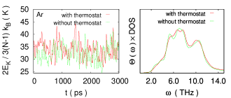
Figure 3: NEMD simulation with $T_{\text{1}}=T_{\text{2}}=20$ K for a 5120 atoms super-cell. Left panel: Twice the kinetic energy per degree of freedom as a function of time. Right panel: vibrational phonon spectrum times DOS [Eq. (III.1)], obtained from the Fourier transform of the velocity auto-correlation function (VAF). Averages were performed over 64 atoms coupled or not to a thermostat.

IV Thermal conductivity

The methodologies introduced in Sec. II were applied to calculate the thermal conductivity of solid argon. This system is well documented in the literature and can be modeled with a simple Lennard-Jones interatomic potential, with parameters $\epsilon/k_{\text{B}}=120$ K and $\sigma=3.4$ Å. All simulations were carried out with the TROCADERO  package. Rurali and Hernández (2003) Super-cells of 256, 1280, 5120 and 10240 atoms were used, and time-steps of 1 or 5 fs. The potential cutoff was fixed to 4$\sigma$.

A comparison of our results to experimental data is shown in Fig. 4. Simulations were performed using either a classical or a quantum thermostat. NEMD was implemented with the two methodologies mentioned above, imposing either a gradient of temperature or a flux of energy. The two methods were in full agreement and are shown here with the same symbols.

NEMD calculations with the quantum thermostat could not be performed below 10 K because of the difficulty to impose or measure a temperature gradient in this temperature range. To measure a temperature gradient, we first compute the profile of kinetic energy across the sample, from which we deduce the classical temperature $T^{\text{C}}$, which serves to map the real temperature $T$ by inverting Eq. (15). At low temperatures however, the classical temperature converges to the zero-point energy and becomes almost temperature independent. Temperature gradients are then difficult to estimate, requiring better statistics, i.e. larger simulation cells and longer simulation times, which limited our calculations to temperatures above about 10 K.

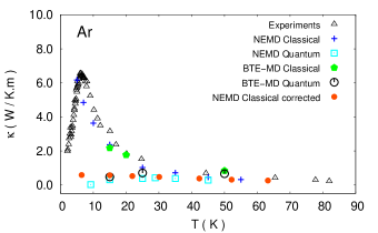
Figure 4: Thermal conductivity of solid argon as a function of temperature. Experimental data reported by Christen and Pollack. Christen and Pollack (1975)

We can see from Fig. 4 that all approaches, classical and quantum, are in good agreement with one another and with experimental data at high temperatures, typically above 40 K.

At lower temperatures, conductivities computed with a classical thermostat remain in good agreement with experimental data Christen and Pollack (1975) down to about 10 K, while the computed quantum conductivities are much lower. Fitting the experimental data to $T^{-n}$, for temperatures higher than 10 K, we find $n=1.23$. Our classical data present, in the same temperature range, a slightly stronger dependence with $n\approx 1.32$. An agreement between classical calculations and experimental data has been obtained as well by other authors, Kaburaki et al. (2007) but is very surprising since quantum effects on the specific heat, which enters directly in the expression of the thermal conductivity [see Eq. (6)], start at about 40 K, as seen in Fig. 2.

The underestimation of the conductivity using the quantum thermostat is not due to an inability of the thermostat to address non-equilibrium conditions, since equivalent results are obtained with the BTE-MD, which is an equilibrium based approach. In NEMD, aside from the phonon-phonon scattering present in real materials, an additional phonon-boundary scattering is present at the boundaries between hot and cold sections (if the system in not large enough). The phonon mean free path is then reduced, i.e. the phonon lifetimes, and a lower thermal conductivity is obtained. At high temperatures such effect is less important, as the mean free path is governed by the phonon-phonon scattering. The phonon population increases with temperature, increasing the phonon-phonon scattering, as more phonons are present to do the scattering. Ashcroft and Mermin (1976) However, the comparison with BTE-MD results suggests that boundary scattering is not the main effect that causes the reduction in thermal conductivity when using the quantum thermostat. Indeed, size effects in BTE-MD are much less important, in the sense that mean free paths are not limited by the boundaries of the system. In this case, a system large enough must be just considered in order to ensure that all modes accessible to the system are well described in the simulation. Our simulations, have been performed for different cell sizes in order to ensure convergence.

Figure 5: Scaled average kinetic energy per mode obtained from MD simulations compared to the correct quantum harmonic distribution given by Eq. (III.1). Crystal argon at 5 K, using a supercell of 256 atoms. The length of the MD simulation was 4 ns.

The inability of the quantum thermostat calculations to describe correctly the thermal conductivity is more probably a consequence of the zero point energy leakage mentioned in Sec. III.2. The main effect of this leakage is that the energy is distributed almost homogeneously among the modes, as in the classical regime, as seen in Fig. 5. The system with the quantum thermostat, hence, behaves almost like a classical system, but at a higher temperature. To illustrate this point, we show in Fig. 6 the evolution of the average phonon lifetime as a function of temperature, obtained with the classical and quantum thermostats. Phonon lifetimes obtained with the quantum thermostat, $\tau^{\text{Q}}$, are much shorter than the classical lifetimes, $\tau^{\text{C}}$, and the former can be obtained from the latter, by replacing the classical temperature $T^{C}$ by its corresponding quantum (real) temperature, $T$ , i.e., we have:

$$\langle\tau^{\text{Q}}(T)\rangle\sim\langle\tau^{\text{C}}(T^{\text{C}})\rangle,$$ (16)

where $T$ and $T^{\text{C}}$ are related by Eq. 15. This correction corresponds to the usual rescaling of temperatures used for instance in Refs. Li et al., 1998 and  Jund and Jullien, 1999b. The agreement between the corrected classical lifetimes and the quantum lifetimes shown in Fig. 6 confirms that the system described with the quantum thermostat is equivalent to a classical system at higher temperature.

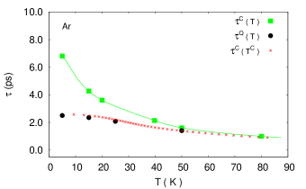
Figure 6: Average phonon lifetimes as a function of temperature obtained from BTE-LD calculations.

Using this insight, the thermal conductivity obtained with the quantum thermostat can be predicted from the classical conductivity. Indeed, if we assume that the specific heat, group velocities and phonon lifetimes are independent, as is often done (see Refs. Li et al., 1998, Jund and Jullien, 1999b), we can approximate Eq. (6) as:

$$\kappa\propto\langle C_{\text{ph}}\rangle\langle\vec{v}_{\text{g}}^{\,2}\rangle\langle\tau\rangle.$$ (17)

We have seen in Sec. III.3 that the quantum thermostat allows to reproduce the average specific heat, so if we assume that the group velocity is not strongly affected by quantum effects, we can write:

$$\kappa^{\,\text{Q}}\large(T\large) = \kappa^{\,\text{C}}\large(T^{\text{C}}\large)\,\frac{C_{\,\text{v}}^{\,\text{Q}}\large(T\large)}{C_{\,\text{v}}^{\,\text{C}}\large(T^{\,\text{C}}\large)}\,\frac{\langle\tau^{\,\text{Q}}\large(T\large)\rangle}{\langle\tau^{\,\text{C}}\large(T^{\,\text{C}}\large)\rangle}$$

$$= \kappa^{\,\text{C}}\large(T^{\,\text{C}}\large)\,\frac{C_{\,\text{v}}^{\,\text{Q}}\large(T\large)}{3\,(N-1)\,k_{\text{B}}},$$

using Eq. (16). The result of this rescaling is shown in Fig. 4, as red full circles. It is seen that this procedure closely matches the conductivities obtained with the quantum thermostat. The correction considered in Eq. (IV), even if it is widely used in the literature, Wang et al. (1990); Lee et al. (1991); Li et al. (1998); Jund and Jullien (1999b) is known to be oversimplified and inaccurate compared to the results of a full quantum approach. Turney et al. (2009a) On the other hand, we have shown here that this correction fully explains the results of the semi-classical Langevin quantum thermostat.

One surprising result remains concerning the apparent absence of quantum effects on the thermal conductivity of argon. Some authors argue that quantum effects are not relevant for argon, even at temperatures well below the Debye value, and avoid any correction. McGaughey and Kaviany (2004a) This simplification is based on the accuracy of the classical theory to describe properties such as the nearest neighbour distance, the bulk modulus, and the cohesive energy of solid noble gases. The effect of neglecting the zero point motion for these properties, is less important in solid argon than in lighter systems. Ashcroft and Mermin (1976) But, from Fig. 2, we know that the heat capacity starts to decrease at about 40 K. From Eq. (17), we see that an absence of quantum effects implies that the decrease in the specific heat is compensated by an increase of the phonon lifetime. However, an exact, or near exact compensation is not expected a priory and seems to be specific to argon, since for instance in Si, classical calculations yield conductivities higher than experimental data. Howell (2012)

V Conclusions

In this work, various methods based on classical or semi classical molecular dynamics were used to obtain the thermal conductivity of a very simple system, solid argon. The results of classical nonequilibrium molecular dynamics, of NEMD using a quantum heat bath, and of the Boltzmann transport equation with lifetimes obtained from molecular dynamics were considered, and compared to experimental data. Very surprisingly, the only method that leads to results in good agreement with experimental data at low temperature is classical molecular dynamics. It must however been admitted that there are good reasons to believe this agreement in the case of Argon is partially fortuitous, and results from a cancellation of errors between heat capacity and phonon mean free path. Indeed, when an empirical description of the heat capacity is introduced in the Boltzmann transport equation, the agreement with experiments worsens. Moreover, other studies in systems such as diamond silicon have shown that the classical MD results can actually strongly overestimate the thermal conductivity at temperatures below the Debye temperature.

The quantum heat bath method, which was originally thought to be promising, as it assigns the correct zero point energy to the phonon modes, leads to a quite poor agreement with experiments, with a strong underestimation of the thermal conductivity. The basic reason for this discrepancy, which appears both in a BTE approach and in a direct nonequilibrium calculation, is a too short lifetime for the vibrational modes. In turn, the latter can be attributed to the zero point energy leakage issue. The vibrational amplitude associated with the zero point energy motion can be exchanged between modes, and can contribute to phonon scattering, which does not correspond to the physical situation in a real quantum system.

A natural question that arises as a result of this work is the existence of a reliable simulation method for computing thermal conductivities in solids below the Debye temperature. Such a method should be able, if one considers the usual formula of Eq. 6, to predict correctly normal mode heat capacities and lifetimes. At present, it appears that no method based on molecular dynamics has the ability to achieve both tasks; classical MD fails on both aspects, while the use of a quantum thermostat results in a strong underestimation of the lifetimes. Ad hoc rescaling of temperatures, or the use of classical phonon lifetimes within a BTE scheme, do not offer any guarantee in terms of reliability or accuracy, although they may work reasonably well for specific systems. For simple crystal systems, a satisfactory alternative is the use of lattice dynamics techniques for computing the phonon lifetimes, based on quantum perturbation theory and using the cubic term in the expansion of the potential energy. Debernardi (1998); Srivastava (1990) Such a method is, however, computationally intensive and tedious. More importantly, it does not seem to be applicable to disordered systems, or even to crystals with complex unit cells. Therefore the calculation of heat conductivity from numerical simulations in such systems at low temperature remains an open challenge.