Dingelstädt/Eichsfeld Prof. Dr. S. K. Solanki Prof. Dr. K.-H. Glaßmeier 4. Februar 2013 2013 3. Mai 2013 2013 978-3-942171-73-1

Investigations of small-scale magnetic features on the solar surface

Vorveröffentlichungen der Dissertation

Teilergebnisse aus dieser Arbeit wurden mit Genehmigung der Fakultät für Elektrotechnik, Informationstechnik, Physik, vertreten durch den Betreuer der Arbeit, in folgenden Beiträgen vorab veröffentlicht:

• T. L. Riethmüller, S. K. Solanki, & A. Lagg, Stratifications of Sunspot Umbral Dots from Inversion of Stokes Profiles Recorded by Hinode, Astrophysical Journal Letters, 678, 157 (2008)

• T. L. Riethmüller, S. K. Solanki, V. Zakharov, & A. Gandorfer, Brightness, distribution, and evolution of sunspot umbral dots, Astronomy & Astrophysics, 492, 233 (2008)

• T. L. Riethmüller, S. K. Solanki, V. Martínez Pillet, J. Hirzberger, A. Feller, J. A. Bonet, N. Bello González, M. Franz, M. Schüssler, P. Barthol, T. Berkefeld, J. C. del Toro Iniesta, V. Domingo, A. Gandorfer, M. Knölker, & W. Schmidt, Bright Points in the Quiet Sun as Observed in the Visible and Near-UV by the Balloon-Borne Observatory Sunrise, Astrophysical Journal Letters, 723, 169 (2010)

• T. L. Riethmüller, S. K. Solanki, M. van Noort, & S. K. Tiwari, Vertical flows and mass flux balance of sunspot umbral dots, eingereicht bei Astronomy & Astrophysics Letters

Inhaltsverzeichnis

1. Summary
2. 1 Introduction
3. 2 Relevant basic physics
   1. 2.1 Phenomena of the solar surface
   2. 2.2 Doppler effect
   3. 2.3 Zeeman effect
   4. 2.4 Polarization of light
   5. 2.5 Radiative transfer
      1. 2.5.1 Fundamental terms
      2. 2.5.2 Spectral line formation
      3. 2.5.3 Polarized radiative transfer
      4. 2.5.4 Inversion of Stokes profiles
   6. 2.6 Magneto-hydrodynamical simulations
      1. 2.6.1 Hydrodynamics
      2. 2.6.2 Magneto-hydrodynamics
      3. 2.6.3 Numerical codes
   7. 2.7 Miscellaneous
      1. 2.7.1 Arcseconds
      2. 2.7.2 Heliocentric angle
      3. 2.7.3 Diffraction limit
4. 3 Review
   1. 3.1 Umbral dots
   2. 3.2 Photospheric bright points
5. 4 Instrumentation
   1. 4.1 The Swedish Solar Telescope
   2. 4.2 The spectropolarimeter aboard the Hinode satellite
   3. 4.3 The balloon-borne observatory Sunrise
      1. 4.3.1 Telescope
      2. 4.3.2 Light distribution and image stabilization
      3. 4.3.3 Software architecture
      4. 4.3.4 Data storage
      5. 4.3.5 Filter Imager
      6. 4.3.6 Imaging magnetograph
6. 5 Brightness, distribution, and evolution of sunspot umbral dots
   1. 5.1 Introduction
   2. 5.2 Observations and data reduction
   3. 5.3 Data analysis
   4. 5.4 Results
      1. 5.4.1 Qualitative results
      2. 5.4.2 Quantitative properties
   5. 5.5 Discussion and conclusions
7. 6 Stratification of sunspot umbral dots
   1. 6.1 Introduction
   2. 6.2 Observations and data reduction
   3. 6.3 Data analysis
   4. 6.4 Inversion results
   5. 6.5 Discussion
8. 7 Vertical flows and mass flux balance of sunspot umbral dots
   1. 7.1 Introduction
   2. 7.2 Observation, data reduction, and analysis
   3. 7.3 Results
   4. 7.4 Discussion and Conclusions
9. 8 Bright points in the quiet Sun as observed by Sunrise
   1. 8.1 Introduction
   2. 8.2 Observations, data reduction, and analysis
   3. 8.3 Results
   4. 8.4 Summary and discussion
10. 9 Comparison of bright points between observations and MHD simulations
    1. 9.1 Introduction
    2. 9.2 Observations, simulations, and degradation
       1. 9.2.1 Observations
       2. 9.2.2 Simulations
       3. 9.2.3 Synthetic instrumental effects
    3. 9.3 Results
       1. 9.3.1 Simulations versus observations: all pixels
       2. 9.3.2 Simulations versus observations: bright points
       3. 9.3.3 Why is the majority of bright points weakly polarized?
       4. 9.3.4 Properties of simulated bright points
    4. 9.4 Discussion
    5. 9.5 Conclusions
11. 10 Outlook
    1. 10.1 Dark lanes and downflow channels of umbral dots
    2. 10.2 Comparison of plage bright points and quiet-Sun bright points
    3. 10.3 Height dependence of the mean downflows in bright points
    4. 10.4 Detailed investigations of synthetic bright points
    5. 10.5 MHD simulations of network bright points
12. A Operator identities
13. Acknowledgments
14. Lebenslauf

Summary

Solar activity is controlled by the magnetic field, which also causes the variability of the solar irradiance that in turn is thought to influence the climate on Earth. The magnetic field manifests itself in the form of structures of largely different sizes, starting with sunspots ($\sim$30000 km), pores ($\sim$5000 km), and micropores ($\sim$1000 km) through to bright points and umbral dots (both $\sim$200 km). The smallest known magnetic features are found to play an important role in the dynamics and energetics of the solar atmosphere. This thesis concentrates on two types of such small-scale magnetic elements: The first part studies the properties of umbral dots, dot-like bright features in the dark umbra of a sunspot. The obtained umbral dot properties provide a remarkable confirmation of the magneto-hydrodynamical simulation results of Schüssler & Vögler (2006). Observations as well as simulations show that umbral dots differ from their surroundings mainly in the lowest photospheric layers, where the temperature is enhanced and the magnetic field is weakened. In addition, the interior of the umbral dots displays strong upflow velocities which are surrounded by weak downflows. This qualitative agreement further strengthens the interpretation of umbral dots as localized columns of overturning convection. The second part of the thesis investigates bright points, which are small-scale brightness enhancements in the darker intergranular lanes of the quiet Sun produced by magnetic flux concentrations. Observational data obtained by the Sunrise mission, having the highest resolution reached for quiet-Sun magnetic field measurements, are used in this thesis. An important part of the work underlying this thesis was the development of the Sunrise Filter Imager (SuFI) software, the reduction of the SuFI data after the flight, the development of fundamental parts of the software for the Instrument Control Unit, and the conceptual design of the Data Storage Subsystem of the Sunrise observatory. With the help of the unique SuFI data, for the first time contrasts of bright points in the important ultraviolet spectral range are determined (this spectral range is of particular relevance for the Sun’s influence on chemistry of the stratosphere). A comparison of observational data with magneto-hydrodynamical simulations revealed a close correspondence, but only after effects due to the limited spectral and spatial resolution were carefully included. 98% of the synthetic bright points are found to be associated with a nearly vertical kilo-Gauss field. A small fraction of the observed bright points with strong polarization signals (most likely corresponding to network elements) cannot be found in the analyzed set of simulations. Larger and deeper computational boxes to include supergranules are suggested for more realistic bright point simulations.

Kapitel 1 Introduction

The Sun as the central star of our solar system is the main energy source from outside Earth and provides all the energy that is necessary to keep the Earth at a temperature needed for higher life. Besides the energetically not so important solar wind and neutrino flux, the main part of the solar energy is provided in the form of electromagnetic radiation. Thus, variations of the insolation were already early assumed to influence climate on Earth. The Serbian mathematician Milutin Milankovitch established a theory now named after him which partly refers cyclic climate variations, in particular the sequence of ice ages to periodic changes in the Earth’s orbit and rotation axis (Milankovitch, 1941). He considered the collective effects of the precession of the Earth’s axis with a period of about 23000 years, the variations in axial tilt (41000 year cycle), and variations in eccentricity (100000 year cycle), calculated variations of the insolation in the range of 5-10%, and held this responsible for the occurrence of the ice ages. In the 1970s, the Milankovitch cycles were confirmed by studies of deep-sea cores which allowed deducing seawater temperatures influenced by glacial periods over about the past 500000 years (Hays et al., 1976; Berger, 1977).

From the theory of stellar evolution it is known that the luminosity of the Sun increased during its lifetime of 4.6 billion years by about 39% (Stix, 2002), but on smaller timescales a constant Sun was assumed for a long time. The total solar irradiance (TSI), i.e. the spectrally integrated solar radiation measured from outside the absorbing terrestrial atmosphere at a distance of 1 AU from the Sun, was hence named solar constant. With the launch of the Earth Radiation Experiment onboard the Nimbus 7 satellite in 1978 (Hoyt et al., 1992), followed by ACRIM I on the Solar Maximum Mission (Willson & Hudson, 1981), the Earth Radiation Budget Experiment onboard the Earth Radiation Budget Satellite (Luther et al., 1986), ACRIM II on the Upper Atmosphere Research Satellite (Willson, 1994), the Solar Variability Instrument on the European Retrievable Carrier (Crommelynck et al., 1993), VIRGO on SOHO (Fröhlich et al., 1997), ACRIM III on ACRIMSat (Willson, 2001), and the Total Irradiance Monitor onboard the SORCE satellite (Kopp & Lawrence, 2005), space-borne radiometers are now operating and measuring the solar irradiance accurately for more than 34 years.

Such measurements revealed that the total solar irradiance varies by about 0.1% coincidentally with the 11-year activity cycle of the Sun (e.g. Fröhlich, 2011; Ball et al., 2012). Surprisingly, the total solar irradiance is highest if the Sun is most active (Willson & Hudson, 1988). This contrasts with the observation that on solar rotational timescales (a month or less) the total irradiance of the Sun is reduced when dark sunspots and pores are present on the solar disk. The reduced luminosity is overcompensated by the bright points (small-scale bright features in the dark interspaces of the granulation) whose number density is increased during the activity maximum (Domingo et al., 2009). Such bright points can be found in high resolution images of the solar surface at all places where the magnetic flux is concentrated into kilo-Gauss elements (Stenflo, 1973; Berger & Title, 2001; Ishikawa et al., 2007). Not much is known about the total solar irradiance variations on timescales of centuries from direct observations, but models provide heavily diverging results, e.g. Krivova et al. (2007).

Technically more challenging than the determination of the total solar irradiance are measurements of the spectral distribution of the solar radiation, since the needed detectors tend to degrade in time, which is difficult to calibrate. Although the TSI varies only weakly over the solar cycle, such measurements revealed that the largest part of the variations are produced at wavelengths shorter than 4000 Å, so that the irradiance in the ultraviolet (UV) can vary by up to a factor of two over the solar cycle, e.g. at the wavelength of Lyman $\mathrm{\alpha}$ (Krivova et al., 2006; Harder et al., 2009). High-resolution observations of bright points with the stratospheric observatory Sunrise (Solanki et al., 2010; Barthol et al., 2011) showed that the bright point contrasts are particularly high in the UV (see chapter 8), so that the radiative properties of the bright points play an important role in influencing irradiance variations and hence possibly the terrestrial climate. Variations in the radiative UV flux can influence the chemistry of the stratosphere, which can propagate into the troposphere and finally change the climate (London, 1994; Larkin et al., 2000; Haigh et al., 2010). Correlations between the solar irradiance variations and climate indicators suggest a causal relation (e.g. Damon & Jirikowic, 1994; Bond et al., 2001). The most noted indication for such a solar forcing of climate change is the so-called Maunder minimum between 1645-1715, where the number of sunspots was extremely low and exceptionally cold winters were observed in Europe and North America (Eddy, 1976; Bradley & Jones, 1993).

One part of this thesis is a small contribution to a better understanding of these photospheric bright points, while the other part addresses a further type of small-scale magnetic structures, the umbral dots, i.e. small bright features inside the dark umbra of sunspots. Umbral dots provide only a negligibly small contribution to the total solar irradiance and hence do not have a noteworthy influence on the terrestrial climate, but they are important for understanding the subsurface energy transport in sunspots. Outside sunspots and pores the energy is transported to the solar surface by convection, which manifests itself in the granulation pattern that is typical for images of the quiet photosphere. The strong and nearly vertical magnetic field of an umbra suppresses convective processes (Biermann, 1941), however, the observed umbral brightness is too high for a completely inhibited energy transport. According to Adjabshirzadeh & Koutchmy (1983), 37% of the radiative umbral flux is provided by umbral dots. Magnetoconvective processes in umbral fine structure, such as umbral dots and light bridges, are assumed to be largely responsible for the umbral energy transport (Weiss et al., 1990; Weiss, 2002).

Physical basics, phenomena, and techniques that are important for the understanding of this thesis, are treated in chapter 2. Chapter 3 gives an overview of the current state of research in the considered fields. Chapter 4 describes the instrumentation which was used for the observations of the following five chapters. The focus is laid on the description of the Sunrise Filter Imager, because the software engineering of this instrument was a significant part of my work in the framework of this thesis. In chapter 5 (published as Riethmüller et al., 2008d), I analyze a time series of a sunspot that was observed with the Swedish Solar Telescope on the Canary Island La Palma. The time series contains thousands of umbral dots, whose analysis yields statistics of lifetimes, sizes, horizontal velocities, peak intensities, and distances travelled over their lifetimes. It is the first extensive statistical umbral dot study of a diffraction-limited time series obtained with an 1-m telescope. The vertical temperature, velocity, and magnetic field structure of umbral dots, as observed with the spectropolarimeter onboard the Hinode satellite, is analyzed in chapter 6 (published as Riethmüller et al., 2008c). For the first time, full Stokes profiles could be inverted for more than two vertical nodes, so that the results could be compared in detail with state-of-the-art magneto-hydrodynamical simulations. A close correspondence with the simulations was found. Chapter 7 refines the analysis of the same Hinode data set by applying a new, considerably improved Stokes inversion technique that greatly reduces the effect of the spatial point spread function of the telescope. For the first time, systematic downflows in the close vicinity of umbral dots could be found in the observations. The results also showed rather well balanced up- and downflow mass fluxes. In chapter 8 (published as Riethmüller et al., 2010), I present the first high resolution observations of the quiet Sun in the near-ultraviolet as observed with the balloon-borne solar telescope Sunrise and I analyze brightness, velocity, and polarization of bright points. The observed bright points are compared with magneto-hydrodynamical simulations in chapter 9 from which new insights into the nature of bright points are obtained. Finally, chapter 10 gives an outlook on how the presented studies on small-scale magnetic features could be usefully continued.

Kapitel 2 Relevant basic physics

The fundamentals, this work relies on, are explained in this chapter. First, the different layers of the solar atmosphere are presented and the solar photosphere is introduced. Examples of the relevant solar surface phenomena are given and the terms used in this thesis are described. Two important effects employed to measure velocities and magnetic fields are explained, the Doppler effect and the Zeeman effect. After an introduction to the Stokes formalism of describing the polarization of light, the topic of radiative transfer in the solar atmosphere is raised and so-called inversion techniques are presented. Inversion is a modern analysis method that has got more and more important within the last years because it helps in retrieving all the significant physical quantities of the solar surface from data that contain spectral as well as polarimetric information. The basic equations used for magneto-hydrodynamical simulations are explained in a further section and finally, the diffraction limit is mentioned since it limits the spatial resolution of every observation with a telescope.

2.1 Phenomena of the solar surface

The Sun is composed of a plasma, i.e. matter containing free electrons and free ions which make the plasma to an electrical conductor. Examples of plasmas are the gas of the flame of a candle, the interstellar medium, or the solar gas. In the case of rigid bodies like planets and moons, it is clear what their surface is. It is not so clear for the Sun because the density of the solar plasma decreases continuously with the radial distance from the center of the Sun, but there is no clear phase transition.

The Sun emits particles (mainly neutrinos, electrons, protons, and neutrons) and electromagnetic waves. Integrated over all wavelengths of the electromagnetic spectrum, a total solar radiation of 1361-1363 watts per square meter (the so-called solar constant) is measured from near-Earth space (Ball et al., 2012). The surface of the Earth is hit by significantly less radiation because the terrestrial atmosphere is not transparent for all wavelengths. The total solar irradiation is $3.8\times 10^{26}$ watt. This huge energy flux originates from the interior of the Sun by nuclear fusion of hydrogen to helium. This fusion zone is also called the core of the Sun and has a temperature of up to 15 million Kelvin and a radius of about 180000 kilometers (Fig. 2.1).

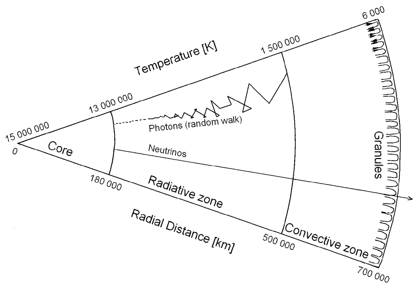
Abbildung 2.1: Internal structure of the Sun. The energy of the Sun is generated in the core by nuclear fusion and then transported by radiation, later by convection to the solar surface. The temperature decreases from 15 million Kelvin in the core to 6000 Kelvin at the top of the convective zone.

The nuclear fusion creates, among others, photons and neutrinos. The neutrinos show hardly any interaction with matter so that they can escape the Sun practically unhindered. The motion of the photons is disturbed all the time by collisions with other plasma particles due to the extremely high plasma density. The photons need up to one million years to leave the Sun. Their mean free path is estimated to be less than a millimeter near the core. The mean free path of the photons increases as the density and temperature decrease on the outside. The energy transport is completely dominated by radiation. This changes at a distance of 500000 kilometers from the center of the Sun. The radiation zone ends there and the convective zone of about 200000 kilometers thickness starts. In this zone, the energy is transported by convection, i.e. plumes of hot gas rise, are cooled, the cooler plasma descends, and the cycle starts again. In the lower photosphere, the convection is visible as the granulation pattern shown in Fig. 2.4. The bright granules, with a typical diameter of 1000 kilometers, are regions of rising hot plasma, the dark regions between the granules (the intergranular lanes) are regions of downflowing cold plasma.

On top of the convective zone, i.e. at a distance of almost 700000 kilometers from the solar center, the plasma density is so low and hence the mean free path of the photons is so large, that they can escape from the Sun. The exact position of this depends on the wavelength of the photons. Almost all the visible light originates from an approximately 500 kilometers thick layer that is called the photosphere. The visible continuum is formed near the bottom of the photosphere which is hence called the solar surface. If more precision is needed, often the solar surface is defined as the position where light from the continuum at 500 nanometer reaches optical depth unity (see section 2.5).

In classical plane-parallel models of the solar atmosphere, the solar plasma reaches its temperature minimum of roughly 4200 Kelvin (Fig. 2.2) at the upper end of the photosphere. Surprisingly, the temperature increases again up to 50000 Kelvin in the adjacent atmospheric layer, the chromosphere, while the plasma density continues to decrease. The chromosphere is about 2000 kilometers thick and is continued by the thin transition region, where the temperature suddenly escalates. Temperatures between one and two million Kelvin are measured in the overlying corona. The corona does not have a sharp outer boundary, but smoothly transits into the solar wind.

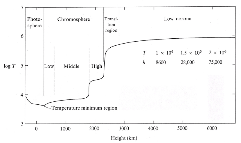
Abbildung 2.2: The solar atmospheric layers and their temperatures. From Athay (1976).

This work studies the electromagnetic radiation that originates from the photosphere. A typical photospheric observation can be seen in Fig. 2.3. It was acquired with the space-borne observatory Hinode at a wavelength of 430 nanometers on 2007 May 2. The field of view is $60\times 70\leavevmode\nobreak\ \mathrm{Mm^{2}}$ and shows a fully developed sunspot and some of its vicinity.

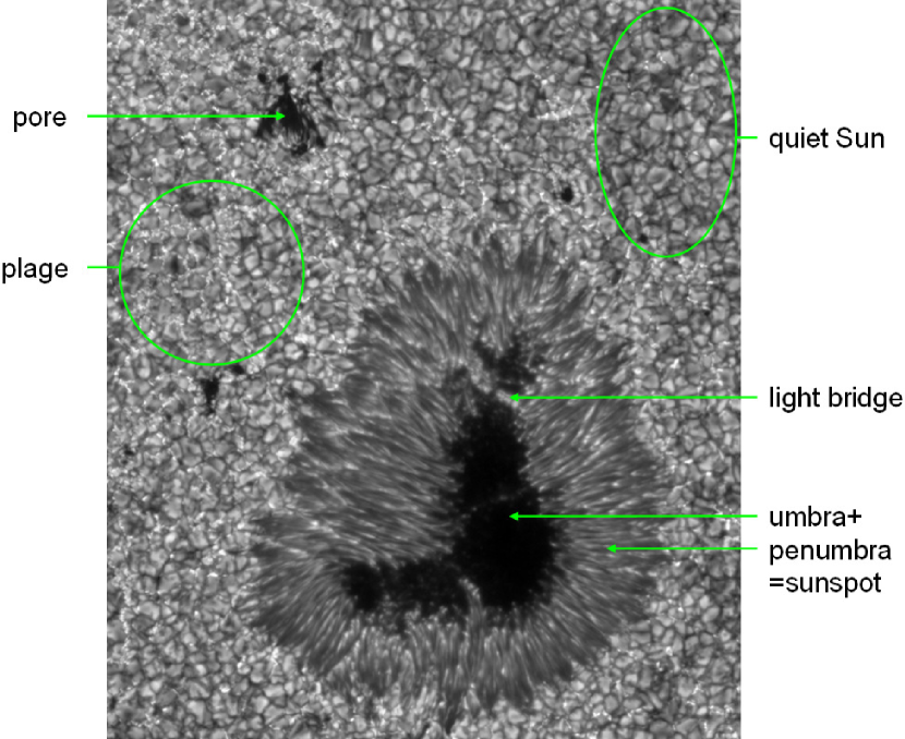
Abbildung 2.3: The solar zoo of the photosphere as observed with the Solar Optical Telescope onboard the Hinode satellite (downloaded from the European Hinode Science Data Center at Oslo University).

The dark region within a sunspot is named the umbra. The outer, slightly brighter region, that consists of many radially oriented filaments, is called the penumbra. A dark region without a penumbra is named a pore. On average, pores are smaller than sunspots. If a pore has a size of only roughly a granule then it is called a micropore. Sometimes a sunspot consists of several umbrae that are separated by light bridges, bright lanes connecting two parts of the penumbra. Outside spots and pores, one can see the granulation in which the convection is manifested as a comblike structure. The dark regions in between the granules are named intergranular lanes, see the enlarged image in Fig. 2.4. Sometimes one can find small roundish brightness enhancements in the darker intergranular lanes - these are bright points. If the granulation pattern contains only a few or hardly any bright points, we call it a quiet-Sun region. In contrast to that, it can happen that the intergranular lanes are strongly filled with bright points, then we refer to it as a plage region. Plage regions are found very often in the vicinity of sunspots. Also the dark pores and umbrae can contain small roundish brightness enhancements called umbral dots.

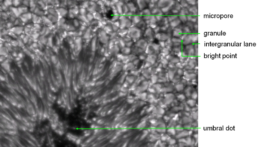
Abbildung 2.4: The tiny features of the photospheric solar zoo.

2.2 Doppler effect

In the lower photosphere, density and temperature of the solar plasma are sufficiently decreased so that the photons coming from the solar interior can escape the Sun (see section 2.1). Some photons interact again with the photospheric gas. Besides electrons, the gas consists of neutral atoms, ions, and molecules. Each of these particles possesses various energy levels. If a photon’s wavelength corresponds to the energy difference between two such levels, the photon can be absorbed by the atom, ion, or molecule. The same particle can later emit a photon of the same energy if it does not collide and get de-excited in that way first. Thus, the many thousand absorption lines in the electromagnetic spectrum of the Sun, also known as Fraunhofer lines, are formed (see also section 2.5.2).

Because of the up- and downflows in the convective zone, the gas of the photosphere is also in motion. If a moving gas cloud emits photons, they exhibit the optical Doppler effect, i.e. a spectral line is shifted. Since typical photospheric velocities are on the order of only a few km/s, it is sufficient to consider the non-relativistic Doppler shift of:

$$\Delta\lambda=\lambda-\lambda_{0}=\lambda_{0}\frac{v_{\rm{LOS}}}{c},$$ (2.1)

where $\lambda_{0}$ is the wavelength at rest, $c$ is the speed of light, and $v_{\rm{LOS}}$ is the line-of-sight (LOS) component (i.e. the component in the direction of the observer) of the cloud velocity. In this thesis, the sign of the velocity is always defined such that negative velocities are upflows (blueshifts). More details about the Doppler effect can be found, e.g., in Grimsehl (1988b) and Bergmann & Schaefer (2004).

The temperature of the gas particles leads to a Maxwell-Boltzmann distribution for their velocities. Since the Doppler effect acts also microscopically, the effect causes a broadening of the spectral lines (Sobel’Man, 1973). If there are upflows and downflows close to each other within the resolution element (or on top of each other along the line-of-sight), then the blue- and redshifts are superimposed macroscopically and can cause an additional line broadening as shown by the green line of Fig. 2.5 for a two-component atmosphere having height independent velocities of $\pm$1.5 km s^-1 using the example of the neutral iron line at 525.02 nm. Since both components are equally strong, the spectral profile remains symmetric. Velocity gradients along the line-of-sight lead to asymmetric profiles. The blue line of Fig. 2.5 exhibits the profile of a one-component atmosphere having a gradient of 2 km s^-1 per $\log(\tau)$ unit.

In the following section, the Zeeman effect is introduced, which can also lead to a line broadening. The question arises how to separate the various reasons for line broadening when observational data are analyzed.

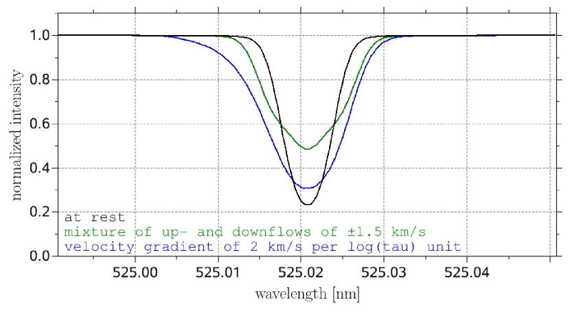
Abbildung 2.5: The influence of the velocity on a spectral line. A mixture of moderate, height independent up- and downflows of equal strength within the resolution element broadens a spectral line. A velocity gradient leads to an asymmetric profile.

2.3 Zeeman effect

The Zeeman effect gives us the possibility to measure the strength and the orientation of magnetic fields on the solar surface. In 1896, the Dutch physicist Pieter Zeeman could confirm the prediction of his colleague Hendrik Antoon Lorentz that many spectral lines split into three components in the presence of a magnetic field (Zeeman, 1897a, b, c, d). Fig. 2.6 gives an example, again for the Fe i line at 525.02 nm. The black line shows the spectral line in the absence of a magnetic field, the green line for a field of 0.3 Tesla (3000 Gauß), a typical field strength in sunspots.

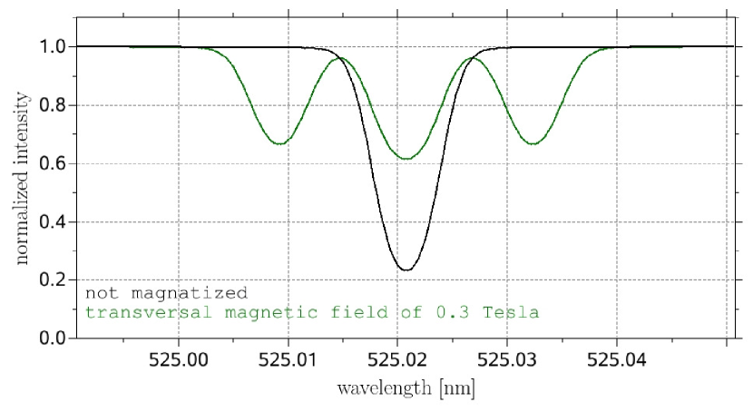
Abbildung 2.6: The influence of a strong, height independent transversal magnetic field on a spectral line. Due to the Zeeman effect, the line is split up into a Lorentz triplet.

A spectral line is formed by the transition of electrons between two energy levels. The quantum numbers $L$ (orbital angular momentum), $S$ (spin angular momentum), and $J$ (total angular momentum) describe the quantum-mechanical state of such energy levels (see e.g. Schwabl, 1992). Without any magnetic field, the energy of an atomic level only depends on the total angular momentum, i.e. on $J$. In the presence of a magnetic field it is:

$$E_{J,M}=E_{J}+\frac{\hbar{}e}{2m_{e}}gMB,$$ (2.2)

i.e. the magnetic field splits the energy level ($L$,$S$,$J$) into $2J+1$ sublevels of slightly different energies. These sublevels are described by the magnetic quantum number $M=-J,..,0,..,+J$. In Eq. (2.2) $\hbar{}=h/2\pi$ means the reduced Planck constant, $e$ is the elementary charge, $m_{e}$ the electron mass, $B$ the magnetic field strength, and $g$ is the Landé factor of the energy level (Landé, 1923; Uhlenbeck & Goudsmit, 1925, 1926), calculated as:

$$g=\frac{3}{2}+\frac{S(S+1)-L(L+1)}{2J(J+1)}.$$ (2.3)

In the case of $J=0$ we also have to set $g=0$.

A negligible magnetic moment of the nucleus is assumed in the Eqs. (2.2) and (2.3) as well as the validity of the LS coupling (also called Russel-Saunders coupling) and that the coupling between the magnetic field and the atom is small compared to the spin-orbit interaction (linear Zeeman effect). In the case of very strong magnetic fields or spectral lines of atoms with a high atomic number, other coupling schemes, the quadratic Zeeman effect, or the Paschen-Back effect have to be taken into account (see, e.g., Sobel’Man, 1973).

The term scheme in Fig. 2.7 illustrates the Zeeman splitting for the iron line at 525.02 nm that is important for chapters 8 and 9. A transition between the energy levels $\mathrm{{}^{5}D_{0}\leftrightarrow{}^{7}D_{1}}$ forms the spectral line. Because of $J=0$, the lower energy level $\mathrm{{}^{5}D_{0}}$ is not degenerated, i.e. it does not split in the presence of a magnetic field. Thanks to $J=1$, the upper energy level splits into three different sublevels with the magnetic quantum numbers $M=-1,0,+1$. A Lorentz triplet is formed, which is named the normal Zeeman effect.

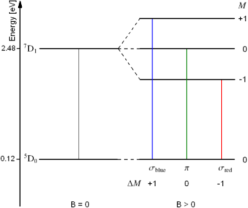
Abbildung 2.7: The normal Zeeman effect using the example of the neutral iron line at 525.02 nm.

A look at Eq. (2.2) reveals that the formation of exactly three splitted lines is not really “normal”, but a particular case that only occurs if either one of the two energy levels of the considered transition has $J=0$ (as shown in the example of Fig. 2.7) or the Landé factors of the two levels are equal. In the general case of the anomalous Zeeman effect, more than three components are observed. For quantum-mechanical reasons not all transitions are allowed. The magnetic quantum number of the two energy levels must not differ by more than one, i.e.:

$$\Delta M=M_{u}-M_{l}=0,\pm{}1,$$ (2.4)

where the indices $l$ and $u$ mean the lower and upper energy level, respectively (see, e.g., del Toro Iniesta, 2003). The anomalous Zeeman effect is illustrated in Fig. 2.8 for the $\mathrm{{}^{5}P_{2}\leftrightarrow{}^{5}D_{2}}$ transition of the iron line at 630.15 nm that is important for chapters 6 and 7. Both energy levels have $J=2$ but differ in the Landé factors, $1.8333$ and $1.5$, so that the line splits into 13 components. The transitions with $\Delta M=0$ are called $\pi$ components, the $\Delta M=\pm{}1$ transitions are the $\sigma_{blue}$ and $\sigma_{red}$ components.

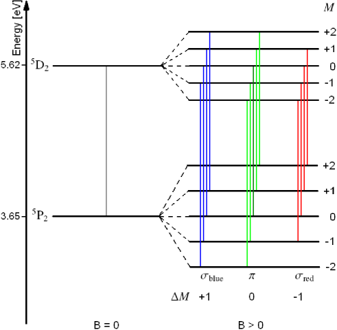
Abbildung 2.8: The anomalous Zeeman effect using the example of the neutral iron line at 630.15 nm.

From Eq. (2.2) follows for the Zeeman line splitting of the transition $l\leftrightarrow{}u$:

$$\Delta\lambda=\lambda-\lambda_{0}=\lambda_{0}\left[\frac{1}{1+\frac{eB\lambda_{0}}{4\pi cm_{e}}(g_{u}M_{u}-g_{l}M_{l})}-1\right],$$ (2.5)

where $\lambda_{0}$ is the reference wavelength of the non-magnetic case. Note that the strength of the various components differs in the general case, which is not further considered here (see, e.g. del Toro Iniesta, 2003; Landi Degl’Innocenti & Landolfi, 2004).

In practice it is often sufficient to calculate the line splitting as a wavelength shift between the center of gravity of the $\sigma$ components, $\lambda_{\sigma}$, to the reference wavelength of the non-magnetic case, $\lambda_{0}$. It is:

$$|\Delta\lambda|=|\lambda_{\sigma}-\lambda_{0}|=\frac{eB\lambda_{0}^{2}}{4\pi cm_{e}}\cdot g_{eff}.$$ (2.6)

The effective Landé factor of the line is defined as (Shenstone & Blair, 1929):

$$g_{eff}=\frac{1}{2}(g_{u}+g_{l})+\frac{1}{4}(g_{u}-g_{l})[J_{u}(J_{u}+1)-J_{l}(J_{l}+1)]$$ (2.7)

and is a measurement for the sensitivity of the spectral line to Zeeman splitting. More details about the Zeeman effect are given by Sobel’Man (1973); Schwabl (1992); del Toro Iniesta (2003); Landi Degl’Innocenti & Landolfi (2004).

The Landé factor of the 525.02 nm line, $g=3$, is one of the biggest Landé factors in the visible spectral range (only the Mn i line at 407.03 nm, the V  i line at 411.66 nm, and the Fe i line at 422.45 nm have higher Landé factors) and therefore makes the line very sensitive to the Zeeman effect, so that even weak magnetic fields in the quiet Sun can be well measured.

Eq. (2.6) reveals that the splitting increases linearly with the magnetic field strength and quadratically with the wavelength, i.e. the splitting is particularly conspicuous in the infrared. Theoretically, the knowledge of the Zeeman splitting allows the determination of the magnetic field strength, but in practice, typical solar surface field strengths lead very often to Zeeman splittings on the order of the Doppler broadening of the spectral lines. Fig. 2.9 displays the weak splitting caused by a 0.07 T (700 G) magnetic field, which cannot be distinguished from the line broadening caused by velocity effects shown in Fig. 2.5 (green line). Also the orientation of the field cannot be determined from the facts mentioned so far.

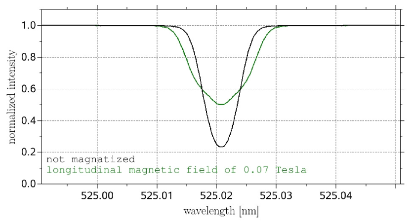
Abbildung 2.9: The influence of a weak, height independent longitudinal magnetic field on a spectral line. The field broadens the line in a quite similar way as the velocity effect illustrated in Fig. 2.5.

Fortunately, it has been shown that the components of the Zeeman splitting are not only wavelength shifted but are also polarized in the following way: If the magnetic field is oriented perpendicular to the line-of-sight (transversal field), the $\pi$ components are linearly polarized parallel to the magnetic field. The $\sigma$ components are also linearly polarized, but perpendicular to the field. If the magnetic field is parallel to the line-of-sight (longitudinal field), the $\sigma_{blue}$- and $\sigma_{red}$ components are oppositely circularly polarized and the $\pi$ components are missing completely (see Fig. 2.10). For arbitrary angles between the magnetic field vector and the line-of-sight, the light of the Zeeman components is elliptically polarized.

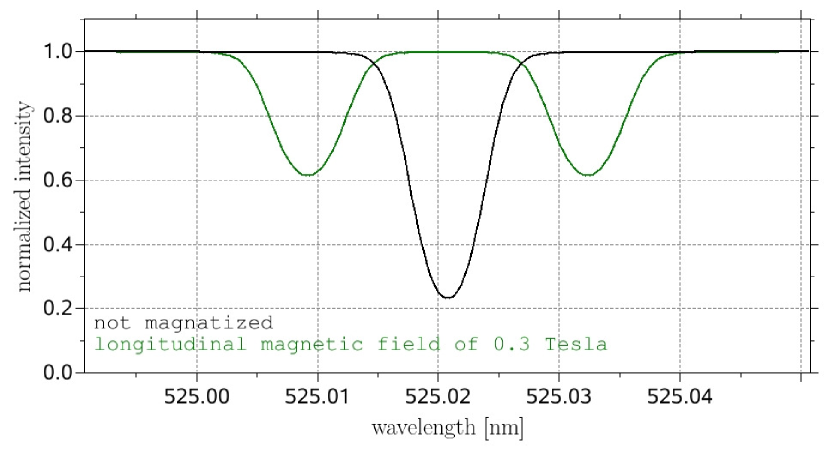
Abbildung 2.10: The influence of a strong, height independent longitudinal magnetic field on a spectral line. The $\pi$ component is not visible since the field is parallel to the line-of-sight.

Because velocity and temperature effects do not lead to a polarization of the light, these effects can be clearly distinguished from magnetic effects by measurements of the polarization properties. The polarization of light shall therefore be treated in more detail in the next section.

2.4 Polarization of light

In 1808, the French engineer and physicist Étienne Louis Malus discovered the broken symmetry of a light beam around its direction of propagation if a glass plate reflects the beam (Malus, 1809). Such an asymmetry of light was never observed before. Fig. 2.11 shows a simplified experimental setup. A common light ray coming from A is reflected by a glass plate $\rm{P_{1}}$ at point B. A second glass plate $\rm{P_{2}}$ makes the broken symmetry visible by reflecting the ray again at point C into direction D. At the beginning, plate $\rm{P_{1}}$ is parallel to $\rm{P_{2}}$ and all rays (i.e. AB, BC, CD) are in one plane. The experiment starts by rotating plate $\rm{P_{2}}$ around the rotational axis BC, so that the ray CD leaves the plane while the rays AB and BC remain in the plane. If the ray reflected by $\rm{P_{1}}$ would be fully symmetrical around its direction of propagation BC, one would always observe a constant brightness for the ray CD for all rotation angles of $\rm{P_{2}}$. This is not the case. One observes a maximal brightness for the rotation angles $\mathrm{0^{\circ}}$ and $\mathrm{180^{\circ}}$, i.e. if the two plates $\rm{P_{1}}$ and $\rm{P_{2}}$ are parallel or antiparallel to each other. A minimal brightness is observed for the rotation angles $\mathrm{90^{\circ}}$ and $\mathrm{270^{\circ}}$. If the experiment is accomplished with monochromatic light and an incidence angle of exactly $\mathrm{56^{\circ}}$, then the brightness goes down to zero. For a glass plate having a refractive index of 1.5, the so-called Brewster angle is $\mathrm{56^{\circ}}$. The Brewster angle is defined as the incidence angle that leads to a reflected ray perpendicular to the refracted ray.

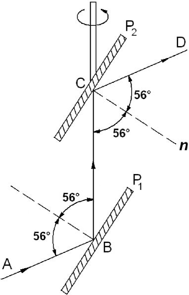
Abbildung 2.11: Experiment to demonstrate the polarization of light due to reflection on a plane surface (from Bergmann & Schaefer, 2004).

Nowadays we know that light exhibits properties of both waves and particles (wave-particle duality). The wave nature of light is described by electromagnetic waves with an electric field vector perpendicular to the magnetic field vector and both vectors are perpendicular to the direction of propagation. Most of the light sources are thermic emitters where the emission processes of a huge amount of atoms are superimposed. Even if a single electron of such a light source can be thought as a simple oscillator, each electron oscillates independently, so that every oscillation direction is equiprobable. Such light is named unpolarized light. The symmetry of unpolarized light around its direction of propagation is of a pure statistical nature. If the atoms of a light source oscillate in only one direction, then the light is linearly polarized. In contrast to the sensory organs of some insects, the human eye has very limited capabilities to distinguish between different states of polarized light (see Haidinger, 1844).

An apparatus creating linearly polarized light is called a linear polarizer, an apparatus to detect linearly polarized light is named an analyzer. In the experiment of Fig. 2.11, the glass plate $\rm{P_{1}}$ serves as a linear polarizer while plate $\rm{P_{2}}$ is the analyzer. What causes the creation of linearly polarized light? As a start, one assumes monochromatic, linearly polarized light hitting the surface of a medium. As indicated in Fig. 2.12, the electric field vector oscillates in the plane of the paper. The electric field of the light source causes oscillations of the medium’s electrons and each oscillating electron is an electric dipole. A dipole cannot radiate into the direction of its oscillation while the radiation perpendicular to its oscillation direction is maximal. If the incident ray hits the surface at the Brewster angle, there is no reflected ray, since it would lie in the oscillation direction of the dipoles. If one assumes that the electric field vector of the incident linearly polarized light oscillates perpendicular to the plane of the paper, then, of course, there is a reflected ray, because this time it is perpendicular to the oscillation direction of the dipoles. Since unpolarized light can be considered as the superposition of linearly polarized light of all possible oscillation directions, it is clear that unpolarized light is partly linearly polarized by a reflection at the Brewster angle.

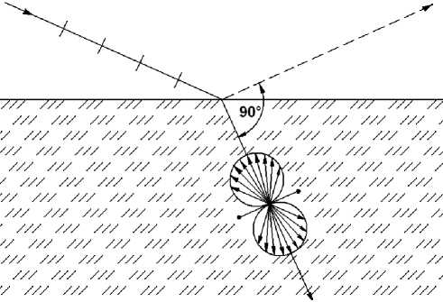
Abbildung 2.12: Illustration of the reflection of linear polarized light under the Brewster angle by the radiation characteristic of a linear oscillating electron (adapted from Bergmann & Schaefer, 2004).

The superposition of two monochromatic linearly polarized light rays whose oscillation directions are perpendicular to each other, results in elliptical polarized light (think of Lissajous figures) depending on the phase between the two. For the particular case of equal amplitudes $E_{x}=E_{y}$ and a phase shift $\Delta$ between the two waves of $90^{\circ}$ ($270^{\circ}$), the ellipse becomes a circle and the light is called left (right) circularly polarized (see Fig. 2.13). For phase shifts of $0^{\circ}$ or $180^{\circ}$, the ellipse becomes a line and the light is again linearly polarized, but with a rotated oscillation direction, which is illustrated in panel a) of Fig. 2.14 for the case of equal amplitudes.

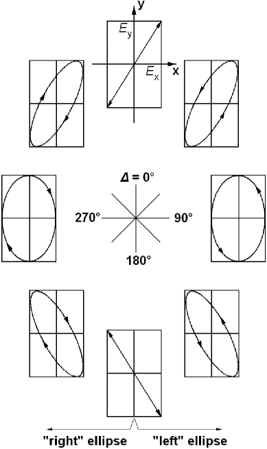
Abbildung 2.13: Elliptical polarized light as the superposition of two linear polarized light beams (adapted from Bergmann & Schaefer, 2004).

Thin plates made of optically biaxial crystals (e.g. glimmer) can be used to rotate the oscillation direction of polarized light. A linearly polarized light ray hits such a retarder plate at an angle of $45^{\circ}$ relative to the two axes of the plate, see Panel b) of Fig. 2.14. According to panel a), the incident light can be thought as a superposition of two linearly polarized light rays whose oscillation directions are perpendicular to each other. Such a retarder plate has different speeds of light along the two axes of the plate, so that the two perpendicular oriented linearly polarized light rays get a phase shift by passing the plate. In the considered case this phase shift is $90^{\circ}$, i.e. $\lambda/4$ (therefore the retarder is called a quarter-wave plate). The incident ray oscillating in the x direction is retarded by $\lambda/4$ compared to the ray oscillating in the y direction, so that the x axis of the quarter-wave plate is named its slow axis and the fast axis is along the y direction. According to Fig. 2.13, the superposition of two linearly polarized light rays of equal amplitudes and a phase shift of $90^{\circ}$ results in circularly polarized light. Thus, a quarter-wave plate can transform linearly polarized light into circularly polarized light and vice versa. Quarter-wave plates are only rarely used in modern polarimeters. Nowadays, liquid crystal retarders are frequently used whose retardance (phase shift between the fast and slow axis) can be voltage-controlled.

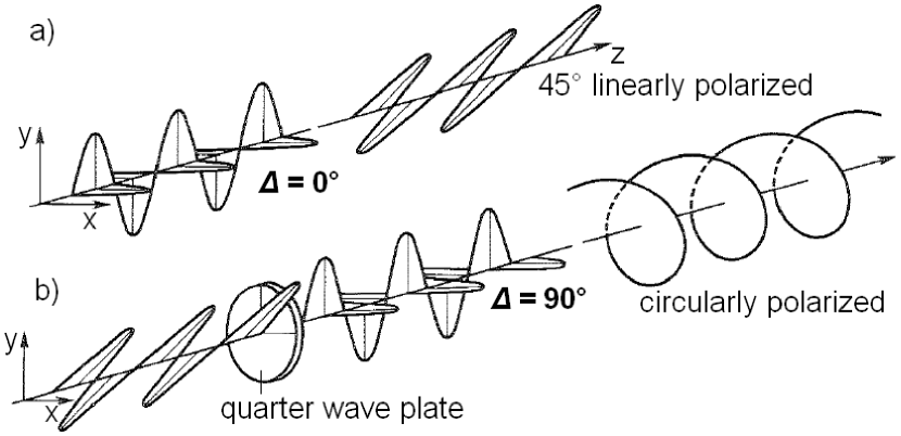
Abbildung 2.14: The rotation of the polarization plane by a quarter-wave plate (from Mayer-Kuckuk, 1985).

The polarization state of light is sufficiently described by two quantities, the amplitude ratio $E_{x}/E_{y}$ and the phase shift $\Delta$. This is reflected in the Jones formalism which describes completely polarized light and its manipulation by optical components, e.g. retarders or linear polarizers, with the help of two-dimensional vectors and matrices (see, e.g., Collett, 1992). In solar physics we practically never deal with completely polarized light but with a mixture of polarized and unpolarized light. For such partly polarized light, the Stokes formalism (Stokes, 1852) has achieved acceptance, in which the polarization state of the light is described by the four-dimensional Stokes vector:

$$\vec{S}=\left(\begin{array}[]{c}I\\ Q\\ U\\ V\end{array}\right).$$ (2.8)

The symbols $I$, $Q$, $U$, and $V$ for the four Stokes parameters were introduced by Walker (1954) and are nowadays commonly used. Stokes $I$ means just the intensity of the light, $Q$ is the intensity difference measured with an ideal linear polarizer at an angle of $0^{\circ}$ and $90^{\circ}$, respectively. The linear polarizer measurements at an angle of $45^{\circ}$ and $135^{\circ}$ lead to Stokes $U$. Finally, Stokes $V$ is the intensity difference measured with a combination of an ideal quarter-wave plate and an ideal linear polarizer at an angle of $45^{\circ}$ and $135^{\circ}$, respectively. Stokes $V$ is hence the difference between the left and right circularly polarized part of the light (see Fig. 2.15). Beyond handling partially polarized light, the Stokes formalism also describes the possibility of determining the state of polarization by just intensity measurements. This is important, since a detector is not able to measure polarization states directly, it can only measure intensities and their differences.

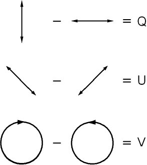
Abbildung 2.15: Schematic representation of the definition of the Stokes parameters. The observer is assumed to face the radiation source (from Landi Degl’Innocenti & Landolfi, 2004).

The ratio of polarized and unpolarized light is expressed by the total polarization degree

$$p=\sqrt{\left(\frac{Q}{I}\right)^{2}+\left(\frac{U}{I}\right)^{2}+\left(\frac{V}{I}\right)^{2}},$$ (2.9)

which can have values from 0 to 1. Completely unpolarized light possesses $Q=U=V=0$ and hence $p=0$, while completely polarized light holds $I^{2}=Q^{2}+U^{2}+V^{2}$, i.e. $p=1$. From the polarization properties of the Zeeman components (see section 2.3) follows that Stokes $V$ displays large signals if vertical magnetic fields are observed at disk center (i.e. the longitudinal case where the field is parallel to the line-of-sight). Large Stokes $Q$ and $U$ signals are found if horizontal fields are observed (transversal case where the field is perpendicular to the line-of-sight). Transverse fields are therefore frequently described by the linear polarization degree

$$p_{lin}=\sqrt{\left(\frac{Q}{I}\right)^{2}+\left(\frac{U}{I}\right)^{2}}$$ (2.10)

and longitudinal fields by the circular polarization degree

$$p_{circ}=\left|\frac{V}{I}\right|.$$ (2.11)

Fig. 2.16 shows Stokes profiles for magnetic fields perpendicular to the line-of-sight. The field strength varies in steps of 0.05 T from 0 (black line) to 0.3 T (3000 G, green line), while the azimuthal orientation of the field with respect to the Stokes $Q$ and $U$ reference direction, $\mathrm{67.5^{\circ}}$, is chosen such that Stokes $Q$ and $U$ have the same amplitude but opposite polarities. The neutral iron line at 525.02 nm serves again as an example. Fig. 2.17 displays the same as Fig. 2.16 but this time the magnetic field is oriented towards the observer. The Stokes $V$ profiles in Fig. 2.17 nicely show the effect of the Zeeman saturation. The amplitude of Stokes $V$ is proportional to the field strength in the case of weak longitudinal fields (a few 100 G). For stronger fields, the $V$ amplitude increases only weakly, while the separation between the red and the blue lobe of the $V$ profile is further proportional to the field strength.

All the magnetic (and velocity) fields we considered so far were constant over all atmospheric heights. As a consequence, all Stokes $I$, $Q$, and $U$ profiles were symmetrical and all $V$ profiles were antisymmetrical. Asymmetrical Stokes profiles require gradients of the magnetic and/or velocity field.

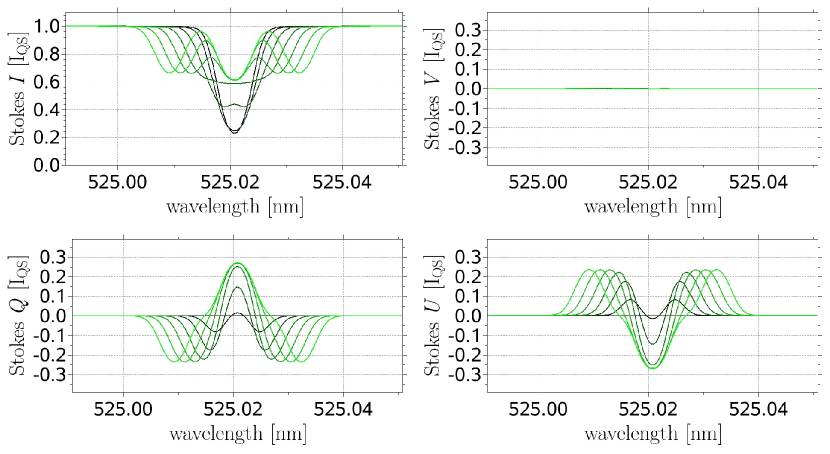
Abbildung 2.16: The influence of a transversal magnetic field on the four Stokes profiles of a spectral line. The height independent field increases from 0 G (black) to 3000 G (green) in steps of 500 G.

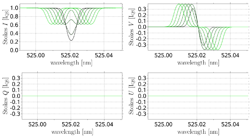
Abbildung 2.17: The same as Fig. 2.16, but for a longitudinal magnetic field.

If a light ray passes a system of optical components, the polarization properties of the light can be influenced by the components, i.e. the incident Stokes vector $\vec{S_{\rm{in}}}$ is transformed into an outgoing Stokes vector $\vec{S_{\rm{out}}}$. Such a transformation can be mathematically described by a multiplication of the so-called Müller matrices by the incident Stokes vector. Imagine a ray to be transmitted through a retarder and then through a linear polarizer, which leads to the following transformation:

$$\vec{S_{\rm{out}}}=M_{\rm{LP}}M_{\rm{Ret}}\vec{S_{\rm{in}}},$$ (2.12)

where $M_{\rm{LP}}$ and $M_{\rm{Ret}}$ are the Müller matrix of the linear polarizer and the retarder. For an ideal linear polarizer, whose transmission direction is identical with the reference direction (e.g. the x axis), the Müller matrix is:

$$M_{\rm{LP}}=\frac{1}{2}\left(\begin{array}[]{cccc}1&1&0&0\\ 1&1&0&0\\ 0&0&0&0\\ 0&0&0&0\end{array}\right)$$ (2.13)

and for an ideal retarder having a retardance of $\Delta$, whose fast axis is identical with the reference direction, it is:

$$M_{\rm{Ret}}=\left(\begin{array}[]{cccc}1&0&0&0\\ 0&1&0&0\\ 0&0&\cos{\Delta}&\sin{\Delta}\\ 0&0&-\sin{\Delta}&\cos{\Delta}\end{array}\right).$$ (2.14)

If an optical component is rotated by the angle $\phi$, the Müller matrix $M_{\rm{0}}$ is transformed into:

$$M_{\rm{\phi}}=M_{\rm{Rot}}(-\phi)M_{\rm{0}}M_{\rm{Rot}}(\phi),$$ (2.15)

where $M_{\rm{Rot}}(\phi)$ is the transformation matrix, which rotates the coordinate system by the angle $\phi$:

$$M_{\rm{Rot}}(\phi)=\left(\begin{array}[]{cccc}1&0&0&0\\ 0&\cos{2\phi}&\sin{2\phi}&0\\ 0&-\sin{2\phi}&\cos{2\phi}&0\\ 0&0&0&1\end{array}\right).$$ (2.16)

Since every telescope and instrument to measure the state of polarization consists of many optical components which change the polarization properties of the light, a way has to be found to disentangle the instrumental polarization from the solar polarization. This problem is solved by a polarimetric calibration that uses calibration optics (often consisting of a rotatable linear polarizer and a rotatable quarter-wave plate) in order to create various well-defined Stokes signals. The modification of the well-known incident Stokes signals by the optical components between the calibration optics and the polarimeter are measured and used to determine the Müller matrix that describes the instrumental polarization. This matrix is also called modulation matrix, its inverse is named demodulation matrix. As part of the data reduction, the Stokes vectors measured during the actual observation (without the calibration optics) are then multiplied by the demodulation matrix so that only the solar polarization remains. One problem of the method is that often the very first components of the optical setup (e.g. primary mirror, entrance lens, coelostat mirrors) cannot be calibrated because it is simply not feasible to mount calibration optics of, e.g., 1-m diameter in front of the telescope. Particularly, plane mirrors can considerably contribute to the instrumental polarization (remember the effect illustrated in Fig. 2.11). Often the part of the telescope that is in front of the calibration optics is theoretically modeled, so that its part of the instrumental polarization can also be removed.

2.5 Radiative transfer

The bulk of our knowledge about the Sun is derived from the emitted electromagnetic radiation. If the radiation passes through the solar atmosphere, its properties change. This change depends on the temperatures, densities, magnetic fields, velocities, etc. of the atmosphere. The theory of the radiative transfer studies the interaction of the radiation with the atmospheric matter in order to retrieve the physical properties of the atmosphere from observed Stokes profiles (Solanki, 1993; Bellot Rubio, 1998; Frutiger, 2000; del Toro Iniesta, 2003).

2.5.1 Fundamental terms

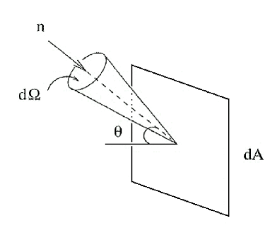
Abbildung 2.18: Illustration of the specific intensity (from Choudhuri, 2010).

Let $dA$ be an infinitesimal small surface element at position ${\bf r}$ of the solar atmosphere (see Fig. 2.18). Furthermore, let ${\bf n}$ be the unit vector in the direction of the observer forming an angle $\theta$ with the surface normal of $dA$. The amount of radiation $dE_{\rm\nu}\,d\nu$ passing through the surface element $dA$ from the solid angle $d\Omega$ in time $dt$ in the frequency interval $\nu,\nu+d\nu$ is proportional to $d\Omega$, $d\nu$, $dt$, and to the projected area $dA\cos\theta$:

$$dE_{\rm\nu}\,d\nu=I_{\rm\nu}\left(\textbf{{r}},t,\textbf{{n}}\right)dt\,d\Omega\,d\nu\,dA\cos\theta$$ (2.17)

The proportionality factor $I_{\rm\nu}$ is named the specific intensity and is a function of the position r, the time $t$, and the direction n. The index ${\rm\nu}$ used for various quantities refers to the frequency dependence. If a body is in thermodynamic equilibrium, i.e. everywhere is the same temperature $T$, it emits black-body radiation which is isotropic and has the specific intensity

$$B_{\rm\nu}\left(T\right)=\frac{2h\nu^{3}}{c^{2}}\frac{1}{\rm{e}^{{\it\frac{h\nu}{k_{\rm B}T}}}-1},$$ (2.18)

where $k_{\rm B}$ is the Boltzmann constant and $B_{\rm\nu}$ is the Planck function (Planck, 1900a, b). Black-body radiation is isotropic and temporally constant if $T$ is constant and hence it depends only on temperature.

If radiation passes through matter, the specific intensity can be changed by two effects. It can be decreased if the radiation is absorbed by the matter or it can be increased if the matter emits radiation. The absorption can be described by an absorption coefficient, $\alpha_{\rm\nu}$, which is proportional to the specific intensity, i.e. the more radiation is present, the more radiation can be absorbed by the matter. $1/\alpha_{\rm\nu}$ gives the mean free path of the photons when passing through the matter. The emission of radiation is described by an emission coefficient, $j_{\rm\nu}$, so that the change of the specific intensity along the ray path is

$$\frac{{\it dI}_{\rm\nu}}{ds}=-\alpha_{\rm\nu}I_{\rm\nu}+j_{\rm\nu}.$$ (2.19)

Eq. (2.19) is called the Radiative Transfer Equation (RTE). The ratio of the emission coefficient to the absorption coefficient

$$S_{\rm\nu}=\frac{j_{\rm\nu}}{\alpha_{\rm\nu}}$$ (2.20)

is named the source function, $S_{\rm\nu}$, so that Eq. (2.19) can also be written as:

$$\frac{{\it dI}_{\rm\nu}}{ds}=-\alpha_{\rm\nu}\left({\it I}_{\rm\nu}-S_{\rm\nu}\right).$$ (2.21)

In the case of non-emitting matter ($j_{\rm\nu}=0$), the radiative transfer equation (2.19) can be solved by a simple integration along the ray path:

$${\it I}_{\rm\nu}\left(s\right)={\it I}_{\rm\nu}\left(s_{0}\right){\rm exp}\left(-\int\limits_{s_{0}}^{s}\alpha_{\rm\nu}(s^{\prime})\,ds^{\prime}\right).$$ (2.22)

This suggests the introduction of the optical depth, $\tau_{\rm\nu}$, as the proper coordinate for radiative transfer problems:

$$\tau_{\rm\nu}=\int\limits_{s_{0}}^{s}\alpha_{\rm\nu}(s^{\prime})\,ds^{\prime},$$ (2.23)

which is equivalent to:

$$\frac{d\tau_{\rm\nu}}{ds}=\alpha_{\rm\nu}.$$ (2.24)

The emission-free solution of the radiative transfer equation is therefore (Choudhuri, 2010):

$${\it I}_{\rm\nu}\left(\tau_{\rm\nu}\right)={\it I}_{\rm\nu}\left(0\right){\rm e}^{-\tau_{\rm\nu}}.$$ (2.25)

If matter only absorbs radiation but does not emit, then the specific intensity of the radiation decreases exponentially. Eq. (2.25) makes clear why $\tau_{\rm\nu}$ is called optical depth. If $\tau_{\rm\nu}\gg 1$ along a ray path through an object, then the light is strongly damped and hence the object is called optically thick (opaque). Accordingly, in the case of $\tau_{\rm\nu}\ll 1$ the object is called optically thin (transparent).

2.5.2 Spectral line formation

Generally, the emission coefficient is not zero and can, just as the absorption coefficient, depend on the frequency and optical depth. (Only time-independent radiation fields are considered here.) A stellar atmosphere whose absorption coefficient, $\alpha_{\rm\nu}$, does not depend on frequency is called a gray atmosphere. In reality, gray atmospheres do not exist. They are just a simplified model which although can be analytically solved (see, e.g., Mihalas, 1970) but cannot explain the formation of spectral lines. The formation of spectral lines can only be described by non-gray atmospheres. The simplest frequency dependence of the absorption coefficient is displayed in panel (a) of Fig.2.19.

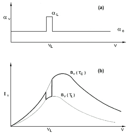
Abbildung 2.19: Illustration of the formation of an absorption line (from Choudhuri, 2010).

In a narrow interval around the frequency $\nu_{\rm L}$, the absorption coefficient has an increased value, $\alpha_{\rm L}$. Outside this interval it has always the value $\alpha_{\rm C}$. (The frequency range outside spectral lines is also called continuum.) It can be shown that the specific intensity at a frequency $\nu$ leaving a stellar atmosphere (e.g. observable with a telescope from near-Earth space) is almost identical with the Planck function (2.18) at an atmospheric depth where the optical depth for that frequency $\nu$ equals unity (Choudhuri, 2010). According to (2.23), the continuum optical depth unity is reached at the depth $\alpha_{\rm C}^{-1}$ having the local temperature $T_{\rm C}$. Hence, the specific intensity for the continuum is $B_{\rm\nu}\left(T_{\rm C}\right)$. Inside the spectral line, the optical depth unity is reached higher up in the atmosphere at $\alpha_{\rm L}^{-1}$ relating to the somewhat lower temperature $T_{\rm L}$, which corresponds to a black-body radiation, $B_{\rm\nu}\left(T_{\rm L}\right)$. The superposition of the two Planck functions results in an absorption line as illustrated by panel (b) of Fig.2.19.

The formation of spectral lines requires a frequency dependent absorption coefficient as well as a temperature gradient in the atmosphere. In the solar photosphere we find a decreasing temperature with height which leads to the formation of absorption lines. At roughly the transition between photosphere and chromosphere, the temperature reaches a minimum and increases again further outwards, see Fig. (2.20). Above the photosphere the temperature gradient reverses its sign so that emission lines are formed.

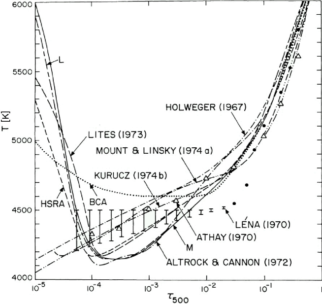
Abbildung 2.20: Temperature as function of the continuum optical depth at 500 nm demonstrating the temperature minimum for various model atmospheres of the Sun (from Vernazza et al., 1976).

2.5.3 Polarized radiative transfer

So far, it was just considered how a stellar atmosphere changes the specific intensity, i.e. Stokes $I$. Not considered was the influence of the atmosphere on Stokes $Q$, $U$, and $V$. As explained in section 2.3, the interpretation of the full Stokes vector is needed to disentangle magnetic and temperature effects and to retrieve the orientation of the magnetic field and not only its strength.

The propagation of electromagnetic radiation in a medium containing a homogeneous magnetic field was formulated in the Stokes formalism for the first time by Unno (1956) for the normal Zeeman effect and provided the first method for a retrieval of the orientation of the magnetic field. Magneto-optical effects influence the Stokes profiles mainly in the core of the spectral lines, which were included in the radiative transfer equations by Rachkovsky (1962). The anomalous Zeeman effect was finally considered by Rachkovsky (1967).

Ignoring the index ${\rm\nu}$ expressing the frequency dependence, Eq. (2.19) can be recast in the generalized form:

$$\frac{\textit{d}\textbf{{I}}}{ds}=-\textbf{{K}}\textbf{{I}}+\textbf{{j}},$$ (2.26)

where I is now the four-dimensional Stokes vector

$$\textbf{{I}}=\left(\begin{array}[]{c}I\\ Q\\ U\\ V\end{array}\right),$$ (2.27)

j stands for the emission vector and K for the total absorption matrix, which consists of a continuum and a line part:

$$\textbf{{K}}=\kappa_{\rm C}\left(\textbf{1}+\boldsymbol{\eta}\right),$$ (2.28)

where $\kappa_{\rm C}$ denotes the continuum absorption coefficient, 1 is the unity matrix, and

$$\boldsymbol{\eta}=\left(\begin{array}[]{cccc}\eta_{\rm I}&\eta_{\rm Q}&\eta_{\rm U}&\eta_{\rm V}\\ \eta_{\rm Q}&\eta_{\rm I}&\rho_{\rm V}&-\rho_{\rm U}\\ \eta_{\rm U}&-\rho_{\rm V}&\eta_{\rm I}&\rho_{\rm Q}\\ \eta_{\rm V}&\rho_{\rm U}&-\rho_{\rm Q}&\eta_{\rm I}\end{array}\right)$$ (2.29)

is the line absorption matrix with only seven independent elements, which meet the following equations:

$$\begin{array}[]{cclcl}\eta_{\rm I}&=&\frac{1}{4}\Big{[}2\eta_{\rm\pi}\sin^{2}{\gamma}&+&(\eta_{\rm\sigma_{blue}}+\eta_{\rm\sigma_{red}})\Big{]}\left(1+\cos^{2}{\gamma}\right)\vspace{3mm}\\ \eta_{\rm Q}&=&\frac{1}{4}\Big{[}2\eta_{\rm\pi}&-&(\eta_{\rm\sigma_{blue}}+\eta_{\rm\sigma_{red}})\Big{]}\sin^{2}{\gamma}\sin{2\chi}\\ \eta_{\rm U}&=&\frac{1}{4}\Big{[}2\eta_{\rm\pi}&-&(\eta_{\rm\sigma_{blue}}+\eta_{\rm\sigma_{red}})\Big{]}\sin^{2}{\gamma}\cos{2\chi}\\ \eta_{\rm V}&=&\frac{1}{2}\Big{[}&&(\eta_{\rm\sigma_{blue}}+\eta_{\rm\sigma_{red}})\Big{]}\cos{\gamma\vspace{3mm}}\\ \rho_{\rm Q}&=&\frac{1}{4}\Big{[}2\rho_{\rm\pi}&-&(\rho_{\rm\sigma_{blue}}+\rho_{\rm\sigma_{red}})\Big{]}\sin^{2}{\gamma}\sin{2\chi}\\ \rho_{\rm Q}&=&\frac{1}{4}\Big{[}2\rho_{\rm\pi}&-&(\rho_{\rm\sigma_{blue}}+\rho_{\rm\sigma_{red}})\Big{]}\sin^{2}{\gamma}\cos{2\chi}\\ \rho_{\rm V}&=&\frac{1}{2}\Big{[}&&(\rho_{\rm\sigma_{blue}}+\rho_{\rm\sigma_{red}})\Big{]}\cos{\gamma}\end{array}$$ (2.30)

The Eqs. (2.26) together with (2.30) are usually named the Unno-Rachkovsky equations. $\gamma$ and $\chi$ denote the inclination and azimuthal angle of the magnetic field vector with respect to the line-of-sight. $\eta_{\rm\pi,\sigma_{blue},\sigma_{red}}$ and $\rho_{\rm\pi,\sigma_{blue},\sigma_{red}}$ are the absorption and dispersion profiles at the wavelength position of the $\pi$, $\sigma_{blue}$, and $\sigma_{red}$ Zeeman components. Details can be found in Bellot Rubio (1998), Frutiger (2000), del Toro Iniesta (2003), or Landi Degl’Innocenti & Landolfi (2004).

For a better understanding, the line absorption matrix can be decomposed in three matrices:

$$\boldsymbol{\eta}=\underbrace{\left(\begin{array}[]{cccc}\eta_{\rm I}&0&0&0\\ 0&\eta_{\rm I}&0&0\\ 0&0&\eta_{\rm I}&0\\ 0&0&0&\eta_{\rm I}\end{array}\right)}_{absorption}+\underbrace{\left(\begin{array}[]{cccc}0&\eta_{\rm Q}&\eta_{\rm U}&\eta_{\rm V}\\ \eta_{\rm Q}&0&0&0\\ \eta_{\rm U}&0&0&0\\ \eta_{\rm V}&0&0&0\end{array}\right)}_{dichroism}+\underbrace{\left(\begin{array}[]{cccc}0&0&0&0\\ 0&0&\rho_{\rm V}&-\rho_{\rm U}\\ 0&-\rho_{\rm V}&0&\rho_{\rm Q}\\ 0&\rho_{\rm U}&-\rho_{\rm Q}&0\end{array}\right)}_{dispersion}$$ (2.31)

where the diagonal absorption matrix only damps the specific intensity of the light but does not change its polarization. The dichroism matrix describes the polarization dependent absorption. Finally, the dispersion matrix expresses the magneto-optical effects which can lead to a redistribution of energy between the states of polarization. Circular birefringence (different refractive indices for left and right circularly polarized light) causes as Faraday effect a rotation of the polarization plane of the linearly polarized part of the light (Faraday, 1855), while linear birefringence (different refractive indices for linearly polarized components of the light that oscillate parallel and perpendicular to the magnetic field) leads as Voigt effect to a phase shift between these components (Wittmann, 1972).

A system is not in thermodynamic equilibrium if the temperature of the system is not unique, e.g. in the case of the solar atmosphere. Nevertheless, there are situations in which the mean free path of the gas particles is small compared to the length scale over which considerable temperature changes occur. Such a situation is named Local Thermodynamic Equilibrium (LTE) and is a valid description, e.g. for the photosphere, which is considered in the following chapters. For the chromosphere and even more for the corona, LTE cannot be assumed. The velocities of the gas particles in an LTE system are Maxwellian distributed, the particle number of the various ionic species is determined by the Saha equation (Saha, 1920) and the population numbers of the participating energy levels can be calculated with the help of the Boltzmann formula (see, e.g., Unsöld, 1968).

The LTE approximation simplifies the determination of the emission vector to:

$$\textbf{{j}}=\kappa_{\rm C}B_{\rm\nu}(T)\left(\begin{array}[]{c}\eta_{\rm I}+1\\ \eta_{\rm Q}\\ \eta_{\rm U}\\ \eta_{\rm V}\end{array}\right)$$ (2.32)

and hence the radiative transfer equation can be written in the form:

$$\frac{\textit{d}}{ds}\left(\begin{array}[]{c}I\\ Q\\ U\\ V\end{array}\right)=-\kappa_{\rm C}\left(\begin{array}[]{cccc}\eta_{\rm I}+1&\eta_{\rm Q}&\eta_{\rm U}&\eta_{\rm V}\\ \eta_{\rm Q}&\eta_{\rm I}+1&\rho_{\rm V}&-\rho_{\rm U}\\ \eta_{\rm U}&-\rho_{\rm V}&\eta_{\rm I}+1&\rho_{\rm Q}\\ \eta_{\rm V}&\rho_{\rm U}&-\rho_{\rm Q}&\eta_{\rm I}+1\end{array}\right)\left(\begin{array}[]{c}I-B_{\rm\nu}(T)\\ Q\\ U\\ V\end{array}\right).$$ (2.33)

Eq. (2.33) is a coupled system of differential equations, which can only be solved analytically for some particular cases. For the general case, the RTE has to be solved numerically. Various numerical RTE codes are available, for example the SIR code (Ruiz Cobo & del Toro Iniesta, 1992; Bellot Rubio, 1998), the STOPRO code (Solanki, 1987; Frutiger, 2000) or the LILIA code (Socas-Navarro, 2001).

2.5.4 Inversion of Stokes profiles

In practice, the use of a numerical RTE code starts with given stratifications of temperature, magnetic field strength and orientation, LOS velocity (and eventually gas pressure) as function of the optical depth for which the numerical solution of the radiative transfer equations provides the synthetic Stokes parameters

$${\textbf{{I}}}^{\rm syn}(\lambda)=\left(\begin{array}[]{c}I^{\rm syn}(\lambda)\\ Q^{\rm syn}(\lambda)\\ U^{\rm syn}(\lambda)\\ V^{\rm syn}(\lambda)\end{array}\right)$$ (2.34)

as a function of the wavelength. For example, the Figs. 2.5 and 2.6 are calculated with such forward calculations, also called syntheses.

In solar physics the inverse problem has often to be solved: An observation campaign provides Stokes parameters at certain wavelength positions within the considered absorption line(s) with the help of a spectropolarimeter. The physical properties of the photosphere need to be retrieved from the observational data. This process is called inversion and starts by making a first guess of the atmospheric parameters, temperature, LOS velocity, magnetic field strength and orientation. The numerical solution of the radiative transfer equations provides synthetic Stokes profiles $\textbf{{I}}^{\rm syn}$, which are then compared with the observed Stokes profiles $\textbf{{I}}^{\rm obs}$. Thus, a merit function

$$\chi^{2}=\sum_{i=1}^{4}{\sum_{j=1}^{N}{\left[\frac{I_{i}^{\rm syn}(\lambda_{j})-I_{i}^{\rm obs}(\lambda_{j})}{\sigma_{i}}\right]^{2}}}$$ (2.35)

can be defined and minimized. (The index $i$ applies to the four Stokes parameters and index $j$ to the wavelength positions. $\sigma_{i}$ denotes the uncertainty in the measurement of the Stokes parameter $i$.) The minimization of the merit function is an iterative process in which the atmospheric parameters are systematically modified (mostly via the Levenberg-Marquardt algorithm, see e.g. Press et al., 2007) until a best fit between synthetic and observed Stokes profiles is reached.

The described inversion technique is applied for each pixel of a one- or two-dimensional map of the solar surface, i.e. the inversion of a pixel is completely independent of the neighboring pixels. Usually, the mentioned first guess of the atmospheric parameters is taken from a model atmosphere for the considered solar surface phenomenon (quiet Sun, plage, umbra) or from the inversion result of a neighboring pixel.

Finally, it is pointed out that the underlying Zeeman effect allows the determination of the magnetic field’s azimuthal direction $\psi$ not completely uniquely because of the ever-present $\mathrm{180^{\circ}}$ ambiguity. From the observed Stokes profiles one cannot distinguish between $\psi$ and $\psi+180^{\circ}$ because both azimuthal angles lead to the same Stokes profile. The inversion retrieves the inclination of the magnetic field vector with respect to the line-of-sight, $\gamma$, and the azimuthal angle in the plane perpendicular to the line-of-sight with respect to the Stokes $Q$ and $U$ reference direction, $\psi$. Usually, the two solutions $(\gamma,\psi)$ and $(\gamma,\psi+180^{\circ})$ are transformed into a coordinate system with respect to the solar surface normal (local reference frame) and often a decision can then be taken which of the two possibilities is the physically meaningful solution (e.g. the orientation of sunspot fields is roughly known). An overview of various algorithms to solve the $\mathrm{180^{\circ}}$ ambiguity can be found in Metcalf et al. (2006).

2.6 Magneto-hydrodynamical simulations

The previous sections 2.1-2.5 concentrated on such aspects of solar physics which are of fundamental importance for an observer of the solar photosphere. Most of the present knowledge about the Sun is retrieved from observations and analyses of the electromagnetic radiation emitted by the Sun towards Earth and analyzed by our instruments from ground, from the stratosphere, or from space. The temporally and spatially highest resolution images stem from light of the photospheric absorption lines in the spectral range 200$-$1600 nm (from the near ultraviolet over the visible to the near infrared). The light of these absorption lines and the associated continuum is emitted by a very thin (compared to the solar diameter) layer of the solar atmosphere of only a few hundred kilometers thickness. The retrieval of information about the deeper layers has proved to be difficult. Even if helioseismology tries to obtain information about the solar interior by measuring solar acoustic oscillations (Gizon & Birch, 2005, 2010), this promising technique cannot yet reach the spatial nor temporal resolution needed to understand the fundamental processes of the interaction between plasma motions and magnetic fields. Also, the theoretical possibility of learning more about the solar core with the help of large neutrino telescopes that collect neutrinos moving practically unhindered from the solar interior towards Earth, is in its infancy (Waxman, 2007; Suzuki & Koshibaa, 2009).

One way out of the dilemma are magneto-hydrodynamical simulations. Magneto-hydrodynamics (MHD) is an important branch of plasma physics, that describes the evolution of a plasma in a macroscopic approximation. A plasma is always assumed to be quasi-neutral, i.e. the negative charges of the electrons are roughly compensated by the positive charges of the ions. Charge separation can be neglected for spatial and temporal scales much larger than the Debye length, $\lambda_{D}=\sqrt{\epsilon_{0}k_{\rm B}T/(e^{2}n_{e})}$ (Debye & Hückel, 1923), and the inverse plasma frequency, $\omega_{P}^{-1}=\sqrt{\epsilon_{0}{}m_{e}/(e^{2}n_{e})}$ (Kippenhahn & Möllenhoff, 1975), respectively, where $\epsilon_{0}$ is the dielectric constant, $k_{\rm B}$ the Boltzmann constant, $T$ the plasma temperature, $e$ the elementary charge, $n_{e}$ the electron number density, and $m_{e}$ the electron mass. Furthermore, the thermal energy of the plasma particles must not exceed the volume charge effects so that a collective behavior of the plasma particles is possible, i.e. the Debye sphere has to contain many electrons, $4\pi\lambda_{D}^{3}n_{e}/3\gg 1$ (Cap, 1994). These conditions are mostly fulfilled in the convective zone and in the lower solar atmosphere, e.g. typical photospheric values, $T=5000\,\mathrm{K}$ and $n_{e}=10^{20}\,\mathrm{m}^{-3}$, lead to $\lambda_{D}=5\cdot 10^{-7}\,\mathrm{m}$, $\omega_{P}^{-1}=2\cdot 10^{-12}\,\mathrm{s}$, and $4\pi\lambda_{D}^{3}n_{e}/3=49$.

2.6.1 Hydrodynamics

In the absence of electromagnetic phenomena, a plasma behaves like a neutral fluid. The dynamic properties of neutral gases and fluids can be described by hydrodynamic equations. In hydrodynamics we distinguish between two kinds of time derivatives of dynamic quantities. The partial derivative of a scalar quantity $Q(\vec{x},t)$ with respect to the time at a fixed position, $\vec{x}$, is called Eulerian derivative and is symbolized, as usual, by $\partial/\partial t$.

$$\frac{\partial Q}{\partial t}=\lim_{\delta t\to 0}\frac{Q(\vec{x},t+\delta t)-Q(\vec{x},t)}{\delta t}.$$ (2.36)

In contrast, $d/dt$ symbolizes the Lagrangian derivative (also named material derivative) and means the temporal variation of a quantity if one moves with the fluid element having the velocity $\vec{v}$.

$$\frac{dQ}{dt}=\lim_{\delta t\to 0}\frac{Q(\vec{x}+\vec{v}\delta t,t+\delta t)-Q(\vec{x},t)}{\delta t}.$$ (2.37)

A first order Taylor expansion of $Q(\vec{x}+\vec{v}\delta t,t+\delta t)$ provides

$$Q(\vec{x}+\vec{v}\delta t,t+\delta t)=Q(\vec{x},t)+\vec{v}\delta t\nabla Q+\delta t\frac{\partial Q}{\partial t}$$ (2.38)

and inserted into Eq. (2.37) it results in

$$\frac{dQ}{dt}=\frac{\partial Q}{\partial t}+\vec{v}\cdot\nabla Q\,,$$ (2.39)

which provides a relation between the Eulerian and Lagrangian derivative. If $\vec{A}$ is a vector field ($\vec{A}=\{A_{i}\}$), Eq. (2.39) becomes in components

$$\frac{dA_{i}}{dt}=\frac{\partial A_{i}}{\partial t}+\sum_{j}{v_{j}\nabla_{j}A_{i}}=\frac{\partial A_{i}}{\partial t}+(\vec{v}\cdot\nabla)A_{i}\,.$$ (2.40)

In hydrodynamics, the conservation of mass is expressed by the continuity equation

$$\frac{\partial\rho}{\partial t}+\nabla\cdot(\rho\vec{v})=0,$$ (2.41)

where $\rho$ stands for the mass density of the fluid. With the help of the product rule for the divergence operator and use of Eq. (2.39), the continuity equation can be written as

$$\frac{d\rho}{dt}+\rho\nabla\cdot\vec{v}=0\,.$$ (2.42)

A fluid is incompressible ($d\rho/dt=0$) if and only if it has a source-free velocity field ($\nabla\cdot\vec{v}=0$).

If we consider incompressible fluids and neglect inner friction (viscosity), the equation of motion for the velocity vector is the Euler equation

$$\rho\frac{d\vec{v}}{dt}=\rho\left(\frac{\partial\vec{v}}{\partial t}+(\vec{v}\cdot\nabla)\vec{v}\right)=-\nabla p+\vec{f}\,,$$ (2.43)

which extends to the Navier-Stokes equation

$$\rho\frac{d\vec{v}}{dt}=\rho\left(\frac{\partial\vec{v}}{\partial t}+(\vec{v}\cdot\nabla)\vec{v}\right)=-\nabla p+\vec{f}+\nabla\hat{\tau}$$ (2.44)

if viscosity and compressibility of the fluid are also considered. $p$ denotes the gas pressure, $\vec{f}$ the force density (unit ${\rm N/m^{3}}$) which acts on the fluid particles, e.g. the gravitational force density $\rho\vec{g}$, and $\hat{\tau}$ is the viscous stress tensor. For incompressible fluids, the viscous term simplifies to $\nabla\hat{\tau}=\mu\Delta\vec{v}$, where $\mu$ is the dynamic viscosity (unit ${\rm Ns/m^{2}}$). More details can be found in the relevant textbooks, e.g. Flügge (1959); Landau & Lifschitz (1974); Greiner (1991a); Choudhuri (1998).

2.6.2 Magneto-hydrodynamics

As the name already expresses, in magneto-hydrodynamics the afore mentioned hydrodynamical equations are generalized by combining them with the electrodynamical equations in order to come to a description of fluids which are good electrical conductors. The Maxwell equations in their usual differential form are written as:

$$\nabla\cdot\vec{D}=\rho_{q}$$ (2.45)

$$\nabla\cdot\vec{B}=0$$ (2.46)

$$\nabla\times\vec{E}=-\frac{\partial\vec{B}}{\partial t}$$ (2.47)

$$\nabla\times\vec{H}=\vec{j}+\frac{\partial\vec{D}}{\partial t}$$ (2.48)

and are complemented by Ohm’s law (see, e.g., Greiner, 1991b; Grimsehl, 1988a):

$$\vec{j}=\sigma\vec{E}.$$ (2.49)

$\vec{E}$ stands for the electric field (unit ${\rm V/m}$), $\vec{D}$ for the dielectric displacement field (unit ${\rm As/m^{2}}$), $\vec{H}$ for the magnetic field (unit ${\rm A/m}$), $\vec{B}$ for the magnetic flux density (also called magnetic induction, unit ${\rm Vs/m^{2}=Tesla=10^{4}}$ Gauß), $\rho_{q}$ for the charge density (unit ${\rm As/m^{3}}$), $\vec{j}$ for the current density (unit ${\rm A/m^{2}}$), and $\sigma$ for the electrical conductivity (unit ${\rm 1/(\Omega m)}$).

A distinction between $\vec{E}$ and $\vec{D}$ or $\vec{B}$ and $\vec{H}$, respectively, makes only sense if one can distinguish between charges and currents in the conductor and its surrounding medium. In the case of plasmas this does not play a role, so that we can write $\vec{D}=\epsilon_{0}\vec{E}$ and $\vec{B}=\mu_{0}\vec{H}$, where $\epsilon_{0}=8.8542\cdot 10^{-12}\,{\rm As/(Vm)}$ is the dielectric constant (permittivity of vacuum) and $\mu_{0}=1.2566\cdot 10^{-6}\,{\rm Vs/(Am)}$ is the magnetic constant (permeability of vacuum). Therefore in astrophysics the magnetic flux density, $\vec{B}$, is often sloppily called the magnetic field. Since the plasma is generally not at rest, but moves with a velocity, $\vec{v}$, the electrostatic force, $q\vec{E}$, acting on a particle of electric charge $q$, has to be extended by the Lorentz force, $q(\vec{v}\times\vec{B})$. The basic suppositions of the MHD approximation are (Kippenhahn & Möllenhoff, 1975; Priest, 1982):

• All plasma velocities are small compared to the speed of light:

  $$\frac{v}{c}\ll 1\,.$$ (2.50)

  Additionally, each temporal variation of a field quantity shall be small in the sense that

  $$\frac{l_{0}/t_{0}}{c}\ll 1\,,$$ (2.51)

  where $l_{0}$ and $t_{0}$ are characteristic spatial and temporal scales on which a field quantity changes.

• The plasma’s electrical conductivity has to be high, so that strong electric fields cannot occur:

  $$\frac{E_{0}}{cB_{0}}\ll 1\,,$$ (2.52)

  where $E_{0}$ and $B_{0}$ are characteristic values of the electric and magnetic field strength.

An order of magnitude estimate of the ratio of the second term on the right-hand side of Eq. 2.48 (displacement current) to the left-hand side of Eq. 2.48 leads to:

$$\frac{\frac{\partial\vec{E}}{\partial t}}{c^{2}\nabla\times\vec{B}}\approx\frac{\frac{E_{0}}{t_{0}}}{c^{2}\frac{B_{0}}{l_{0}}}=\frac{E_{0}}{cB_{0}}\cdot\frac{l_{0}/t_{0}}{c}\ll 1\,,$$ (2.53)

so that displacement currents can be neglected (see also Cap, 1994; Choudhuri, 1998). Hence, the Eqs.(2.45)-(2.49) can be simplified:

$$\nabla\cdot\vec{E}=\frac{\rho_{q}}{\epsilon_{0}}$$ (2.54)

$$\nabla\cdot\vec{B}=0$$ (2.55)

$$\nabla\times\vec{E}=-\frac{\partial\vec{B}}{\partial t}$$ (2.56)

$$\nabla\times\vec{B}=\mu_{0}\vec{j}$$ (2.57)

$$\vec{j}=\sigma(\vec{E}+\vec{v}\times\vec{B})\,.$$ (2.58)

Eq. (2.58) inserted into Eq. (2.57) results in

$$\vec{E}=\eta\nabla\times\vec{B}-\vec{v}\times\vec{B}\,,$$ (2.59)

where $\eta=1/(\mu_{0}\sigma)$ denotes the magnetic diffusivity. Therefore, the electric field vector is not an independent dynamic variable of magneto-hydrodynamics, but it can be calculated from the magnetic field $\vec{B}$ and the velocity $\vec{v}$. The only one new dynamic variable is the magnetic field vector, $\vec{B}$, whose temporal evolution has to be described by a further equation. Thereto, Eq. (2.59) is inserted into Eq.(2.56) and assumed that the electrical conductivity, $\sigma$, is spatially constant. With the help of the operator identity (A.4) and Eq. (2.55), we can derive the induction equation

$$\frac{\partial\vec{B}}{\partial t}=\nabla\times(\vec{v}\times\vec{B})+\eta\Delta\vec{B}\,.$$ (2.60)

Besides this new equation for the magnetic field, the above mentioned hydrodynamical equations (2.41) and (2.44) are still valid but have to be extended by the magnetic field. The continuity equation (2.41) remains but the Navier-Stokes equation (2.44) has to be extended by the magnetic force density $\vec{j}\times\vec{B}$ (see, e.g., Gerthsen et al., 1992; Grimsehl, 1988a)

$$\rho\left(\frac{\partial\vec{v}}{\partial t}+(\vec{v}\cdot\nabla)\vec{v}\right)=-\nabla p+\vec{j}\times\vec{B}+\rho\vec{g}+\nabla\hat{\tau}\,,$$ (2.61)

which, after using Eqs.(2.57) and (A.5), results in the following MHD equation of motion:

$$\rho\left(\frac{\partial\vec{v}}{\partial t}+(\vec{v}\cdot\nabla)\vec{v}\right)=-\nabla\left(p+\frac{B^{2}}{2\mu_{0}}\right)+\frac{(\vec{B}\cdot\nabla)\vec{B}}{\mu_{0}}+\rho\vec{g}+\nabla\hat{\tau}\,.$$ (2.62)

The presence of a magnetic field leads to an additional magnetic pressure of the form $B^{2}/(2\mu_{0})$ (in the cgs system: $B^{2}/(8\pi)$). The ratio of the thermal to the magnetic pressure

$$\beta=\frac{\mathrm{thermal\leavevmode\nobreak\ pressure}}{\mathrm{magnetic\leavevmode\nobreak\ pressure}}=\frac{2\mu_{0}p}{B^{2}}$$ (2.63)

plays an important role in the investigation of magneto-hydrodynamical phenomena. In the case $\beta\gg 1$, e.g. in the convective zone, the gas plays the important role and forces the magnetic field lines to follow the gas motions. On the other hand, in the case $\beta\ll 1$, e.g. in the solar corona, the magnetic field dominates the dynamic behavior of the plasma. The plasma particles have to follow the magnetic field. $(\vec{B}\cdot\nabla)\vec{B}/\mu_{0}$ is the second term of Eq. (2.62) which is of a magnetic nature. It is a magnetic tension along the field lines.

The conservation of energy can be expressed in terms of the total energy per unit volume, $e$ (unit ${\rm J/m^{3}}$), which is the sum of the internal energy density, the kinetic energy density, and the magnetic energy density: $e=e_{\rm int}+\rho v^{2}/2+B^{2}/2\mu_{0}$. The time derivative of this energy balance as well as the use of the induction equation (2.60) and the equation of motion (2.62) lead to the MHD energy equation (Vögler, 2003; Vögler et al., 2005):

$$\frac{\partial e}{\partial t}+\nabla\cdot\left[\vec{v}\left(e+p+\frac{|\vec{B}|^{2}}{2\mu_{0}}\right)-\frac{1}{\mu_{0}}\vec{B}(\vec{v}\cdot\vec{B})\right]=\\ \frac{1}{\mu_{0}}\nabla\cdot(\vec{B}\times\eta\nabla\times\vec{B})+\nabla\cdot(\vec{v}\cdot\hat{\tau})+\nabla\cdot(K\nabla T)+\rho(\vec{g}\cdot\vec{v})+Q_{\rm rad}\,,$$ (2.64)

where $K$ stands for the thermal conductivity (unit ${\rm W/(mK)}$) and $T$ for the temperature. $Q_{\rm rad}$ takes into account radiation heating and cooling processes and requires radiative transfer calculations.

The relations between the thermodynamic quantities of the plasma are described by the equations of state, e.g. in the form $T=T(\rho,e_{\rm int})$ and $p=p(\rho,e_{\rm int})$ and complete the system of MHD equations (2.41), (2.60), (2.62), (2.64). Derivations and examples of physical applications of the MHD equations can be found in, e.g., Priest (1982); Cap (1994); Choudhuri (1998).

2.6.3 Numerical codes

Subject of this study is the investigation of solar photospheric phenomena. Such phenomena often have their origin in the convective zone or are determined by the interplay of the convection zone with the photosphere. Since the convective zone eludes a direct observation, the development of numerical codes is pursued, which simulate the behavior of the plasma in the convective zone and photosphere by solving the MHD equations. If the simulation results agree well with the photospheric observations, there is hope that the simulations can also reproduce the behavior of the convective zone. Numerical MHD codes do not only give the physicists the possibility to look below the solar surface, but they also provide results at an arbitrarily high temporal, spatial, and spectral resolution as well as free of stray light and noise.

In the transition from the convective zone to the photosphere, the plasma density is sufficiently decreased, so that the plasma becomes transparent for wavelengths in the visible spectral range. The convective energy transport changes into a radiative energy transport. The irradiance emitted by the Sun as well as the temperature profile of the photosphere depend on the energy exchange between gas and radiation. Therefore, the energy equation of a numerical code simulating the photosphere has to comprise a radiative term, i.e. the radiative transfer equation has also to be solved numerically. Such a code is called a radiation MHD code.

Examples of numerical radiation MHD codes are the MURaM code (Vögler, 2003; Vögler et al., 2005), the CO⁵BOLD code (Freytag et al., 2008, 2012), or the Stagger code (Nordlund & Galsgaard, 1995; Galsgaard & Nordlund, 1996). A comparison of the results of these three codes can be found in Beeck et al. (2012).

2.7 Miscellaneous

2.7.1 Arcseconds

A solar physicist says, an object of the solar surface has a size of one arcsecond, if the object has an angular resolution of $1/3600^{\circ}$ when observed from Earth. The conversion between arcsecond and kilometer depends on the distance between Earth and Sun, which varies in the course of a year. Algorithms to calculate the Earth-Sun distance can be found in Meeus 1991, source codes of an implementation using the programming language C++ are part of Hirzberger & Riethmüller 2009. Hence, an arcsecond corresponds to 713 km - 737 km on the solar surface. Averaged over the year, one finds: 1^′′ = 725 km. When Sunrise observed the data used in chapter 8 and 9, the relation was: 1^′′ = 736.4 km.

The Sun has a radius of R = 696 000 km and the mean distance to Earth is D = 149 600 000 km (see Fig. 2.21). If observed from Earth, the solar diameter, $\alpha$, is in arcseconds: $\tan{(\alpha/2)}=R/D$, hence $\alpha=2\arctan{(R/D)}=0.533^{\circ}=32\mbox{${}^{\prime}$}=1919\mbox{${}^{\prime\prime}$}$.

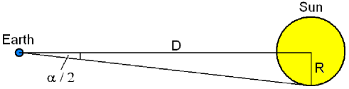
Abbildung 2.21: Viewing angle of the Sun as observed from Earth.

2.7.2 Heliocentric angle

Since the Sun is a sphere, we only look perpendicularly through the solar atmosphere if the observed phenomenon is located in the center of the solar disk. In the case of off-center observations, the line-of-sight is inclined with respect to the solar surface normal. This leads to projection effects which are more pronounced close to the solar limb. Often the heliocentric angle of the observed region, i.e. the angle between the line-of-sight (direction to the observer) and the surface normal, is given to quantitatively capture the strength of such projection effects. The left panel of Fig. 2.22 exhibits the Sun as it was observed on September 9, 2004. The sunspot S of active region NOAA 10667 (extensively analyzed in chapter 5) was two days after our observation at the Swedish Solar Telescope at the position $x=479\mbox{${}^{\prime\prime}$},\leavevmode\nobreak\ y=-280\mbox{${}^{\prime\prime}$}$. The distance between S and disk center was therefore $r=\sqrt{x^{2}+y^{2}}=555\mbox{${}^{\prime\prime}$}$. The right panel of Fig. 2.22 shows a cut through the plane spanned by $r$ and the LOS, with the observer being on the right side. The heliocentric angle can be calculated as follows:

$$\sin{\theta}=\frac{\sqrt{x^{2}+y^{2}}}{R},$$ (2.65)

where $R=1919\mbox{${}^{\prime\prime}$}/2$ denotes the solar radius in arcseconds. Often the value $\mu=\cos{\theta}$ is given.

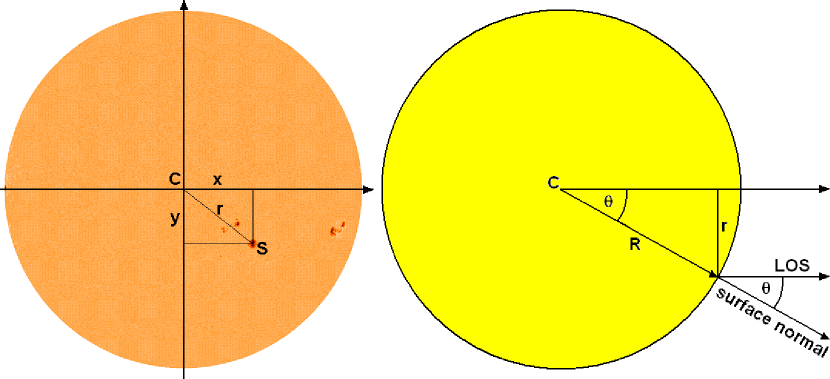
Abbildung 2.22: Definition of the heliocentric angle $\theta$ as angle between the line-of-sight (LOS) and the surface normal.

2.7.3 Diffraction limit

If light enters a telescope, the wavefront is restricted, mostly by the size of the main mirror or, in case of a refractor, by the size of the entrance lens. Hence, the light is diffracted at the border of the entrance aperture, i.e. a point-like object (e.g. a star) is imaged by a telescope as an Airy disk instead of a point. If two nearby point sources are observed, the two Airy disks are superimposed and cannot be separated if their distance is sufficiently small. According to the so-called Rayleigh criterion, two point sources can be separated if their distance is at least the radius of the Airy disk, i.e. if the first minimum of the one Airy disk is at the position of the maximum of the other Airy disk. The corresponding angular resolution is:

$$\sin{\alpha}=1.22\frac{\lambda}{D},$$ (2.66)

where $\lambda$ stands for the observed wavelength and $D$ for the diameter of the telescope’s entrance aperture. Hence, the spatial resolution of a telescope is better for larger telescopes and for shorter wavelengths. At a wavelength of 6301.5 Ångström, the 50-cm telescope SOT onboard the Hinode satellite (see chapters 6 and 7) has a diffraction limit of $\alpha=\arcsin{(1.22\times 6301.5\times 10^{-10}\,\mathrm{m}\,/\,0.5\,\mathrm{m})}=0.0000979^{\circ}=0$$\mbox{.}^{\prime\prime}$$35=255$ km. For the shortest wavelength of Sunrise (see chapters 8 and 9), the diffraction limit is $\alpha=\arcsin{(1.22\times 2140\times 10^{-10}\,\mathrm{m}\,/\,1.0\,\mathrm{m})}=0$$\mbox{.}^{\prime\prime}$$05=40$ km.

Kapitel 3 Review

After the outline, in Chapter 2, of the physical basics essential for the understanding of this thesis, this chapter reviews the historical development of research on small-scale magnetic features. An overview of the most important umbral dot studies is given first, followed by the papers on bright points. Completeness cannot be claimed owing to the large number of publications on these topics. Instead the review is restricted to such aspects that are relevant for this thesis.

3.1 Umbral dots

Bright sub-structures inside a sunspot umbra were observed for the first time by Father Stanislas Chevalier in 1907 (see Chevalier, 1914a, 1916a, and also Fig. 3.1). The leader of the Jesuitian observatory near Shanghai discovered with a 40-cm refractor a small-scale granulation-like pattern in the umbra which appeared more coarse than the quiet-Sun granulation (Chevalier, 1916b). In 1941, Ludwig Biermann stated, that strong magnetic fields in sunspots suppress the convection by eddy-current braking (Biermann, 1941). In a sunspot, the energy can only be transported by radiation but not by convection. In 1950, Georg Thiessen confirmed the umbral granulation observed by Chevalier with the 60-cm refractor of the observatory of Hamburg-Bergedorf (Thiessen, 1950). He found a mean diameter of an umbral granule of 1^′′, while the size of a typical photospheric granule was 1$\mbox{.}^{\prime\prime}$3. Sometimes the umbra did not show a granulation pattern, instead he found bright dots inside the umbra of only 0$\mbox{.}^{\prime\prime}$3. In 1959, Bray & Loughhead determined for the first time the lifetime of umbral granules and found values between 15 and 120 minutes (Bray & Loughhead, 1959; Loughhead & Bray, 1960). Since their telescope, having an aperture of 12.7 cm, had only a limited spatial resolution and the seeing was probably not optimal, they only found large values of 2$\mbox{.}^{\prime\prime}$3 and 2$\mbox{.}^{\prime\prime}$9 for the mean size of granules in the umbra and quiet Sun, respectively.

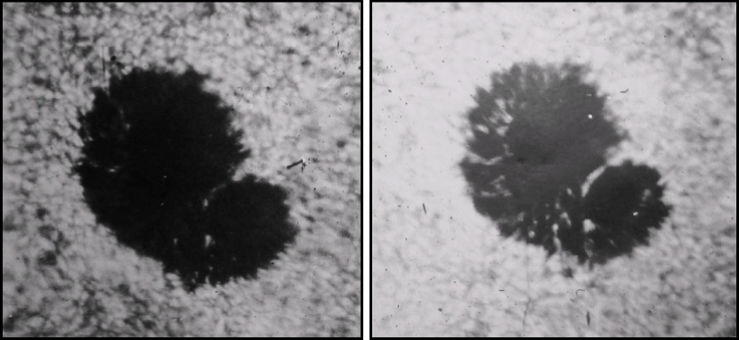
Abbildung 3.1: Bright features visible in the dark umbra of a sunspot observed by the Jesuit Stanislas Chevalier in 1907 with a 40-cm refractor at the ground-based observatory of Zô-Sè close to Shanghai (Chevalier, 1916a). The solar scene was photographed twice with a different exposure time.

The early observations were made from ground and without using adaptive optics, hence they suffered from variable seeing conditions. The situation changed with the launches of the balloon-borne 30-cm telescope Stratoscope I in the years 1957-1959 (Rogerson, 1958; Danielson, 1961). The flight on September 24, 1959 concentrated on umbral observations. Danielson (1964) introduced the name umbral dot (UD) for the small-scale bright dots inside umbrae and argued that the so-called umbral granulation does not really exist but is only the result of observations of UD groups at insufficient spatial resolution or under poor seeing conditions, respectively (see Fig. 3.2). He could only limit the UD lifetimes roughly between 4 and 50 minutes owing to the small number of observations. This range of UD lifetimes was consistent with the lifetimes of umbral granules found by Loughhead & Bray (1960). Observations with the 30-cm telescope of the Sacramento Peak Observatory confirmed that the bright umbral sub-structures are not closed patterns like in the quiet Sun but rather isolated emission dots (Beckers & Schröter, 1968b).

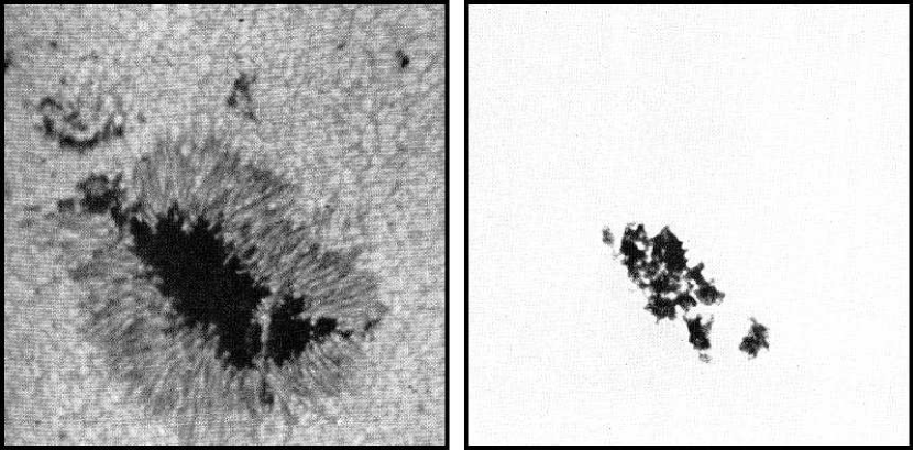
Abbildung 3.2: Umbral dots observed with the balloon-borne 30-cm telescope Stratoscope I in 1959 (Danielson, 1964). The solar scene was photographed twice with a different exposure time.

Spectroscopical observation methods finally provided information about the magnetic field strength and LOS velocity of the UDs. Kneer (1973) found a field weakening from 2600 G in the umbral vicinity to 1200 G in the observed UD. Considerably lower field weakenings of only 5-20% are reported, e.g., by Buurman (1973); Adjabshirzadeh & Koutchmy (1983); Pahlke & Wiehr (1990); Schmidt & Balthasar (1994); Tritschler & Schmidt (1997). On the contrary, other authors did not find indications of magnetic field weakenings in UDs (see, e.g., Zwaan et al., 1985; Lites & Scharmer, 1989; Lites et al., 1991), but used only Stokes $I$ observations of single spectral lines, which limited the accuracy of their results. Schmidt & Balthasar (1994) pointed out, that a field weakening of 5-20% can also be explained by the fact that the magnetic field in a sunspot decreases with height and that the visible surface of an UD is enhanced compared to its vicinity, see Fig. 3.3. According to Parker (1979) and Choudhuri (1986), the UDs are seen as thin columns of field-free hot gas penetrating the cluster of small magnetic flux tubes that form the sub-photospheric structure of a sunspot. In addition to the cluster model, a second sunspot model exists. In the monolithic model, sunspots are homogeneous even below the solar surface. Numerical simulations revealed that magneto-convective processes in such strongly magnetized plasmas can lead to spatially modulated oscillations, that possibly can be observed as UDs (Weiss et al., 1990; Hurlburt et al., 1996).

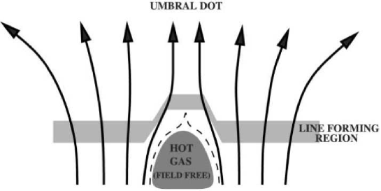
Abbildung 3.3: Sketch of an umbral dot as an intrusion of field-free hot gas in between a bundle of thin magnetic flux ropes of the cluster model of sunspots. The increased temperature of the UD shifts the line forming region (shaded) to higher layers. From Socas-Navarro et al. (2004).

A similar heterogeneous picture was found for the LOS velocities of UDs. While Kneer (1973) and Pahlke & Wiehr (1990) determined upflow velocities in the range 1-3 km s^-1, Rimmele (1997), Hartkorn & Rimmele (2003) and Socas-Navarro et al. (2004) found only small blueshifts of 50-300 m s^-1. Zwaan et al. (1985), Schmidt & Balthasar (1994) and Wiehr (1994) could not retrieve any vertical plasma flows in the UDs relative to their surroundings. Besides insufficient spatial resolution, there are further reasons for the diversity of the results: On the one hand, the observations were done in various spectral lines, which are formed in different atmospheric heights. Since the field lines of the umbral magnetic field show a canopy-like structure above the UD (see below), the measured field weakening (and LOS velocity) depends strongly on the formation height of the used spectral line. On the other hand, the observations could be influenced by varying atmospheric seeing conditions and different levels of stray light contamination.

Among the most comprehensive UD analyses are those of Sobotka et al. (1997a, b). With the Swedish 50-cm telescope (SVST), an umbra could be observed for 4.5 hours under outstanding seeing conditions. The analysis of 662 observed UDs revealed monotonically decreasing histograms for UD lifetime and effective diameter. On average, an UD lived 13.8 minutes and had a diameter of 0$\mbox{.}^{\prime\prime}$42. The UDs moved horizontally with velocities in the range of 0-1000 m s^-1, where the UD speeds were slightly grouped at 100 m s^-1 and 400 m s^-1. Large and long-lived UDs were preferentially found near the umbral border. Sobotka & Hanslmeier (2005) repeated the determination of the UD diameters with the now upgraded 1-m Swedish telescope (SST) and found a maximum in the histogram at 0$\mbox{.}^{\prime\prime}$23. While more recent UD studies only investigated individual UD properties and did not determine, e.g., UD trajectories (Tritschler & Schmidt, 2002; Hartkorn & Rimmele, 2003; Sobotka & Hanslmeier, 2005), chapter 5 extends the work of Sobotka et al. by analyzing a multitude of UD properties (e.g. lifetimes, diameters, horizontal velocities, peak intensities) of an almost two-hour SST time series of photometric sunspot data. For the first time, the observations with a 1-m telescope were brought very close to the theoretical diffraction limit of 0$\mbox{.}^{\prime\prime}$18 at the observing wavelength with the help of a modern image reconstruction technique (Multi-Frame Blind Deconvolution, Löfdahl, 2002).

A substantial step in the understanding of UDs was taken with the help of MHD simulations. The realistic simulation of three-dimensional radiative magneto-convection of an umbra by Schüssler & Vögler (2006) yielded numerous UDs as a natural consequence of the convection in a strong, initially monolithic, magnetic field. Upflows of hot gas are present inside the synthetic UDs and narrow downflow channels surround the UDs. Close to the visible surface, the magnetic field of the UDs is significantly weakened (see Fig. 3.4). Most of the UDs are slightly elongated in the horizontal direction and show a central dark lane. At least for relatively large UDs, the dark lanes predicted by the simulations were found in the observations of Bharti et al. (2007) and Rimmele (2008).

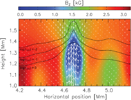
Abbildung 3.4: Vertical cut trough an UD as simulated by Schüssler & Vögler (2006). Colors indicate magnetic field strength, and the arrows represent (projected) velocity vectors. The longest arrow corresponds to a velocity of 2.7 km s^-1. The black lines indicate levels of constant optical depth $\log(\tau_{500})=0$, $-1$, and $-2$ (bottom to top). The upper part of the plume has developed a cusplike shape with a strongly decelerated upflow and a weak magnetic field.

Another important milestone in the investigation of UDs was the introduction of inversion techniques for analyzing Stokes profiles (see section 2.5.4). Older analyses of spectroscopic data retrieved the magnetic field strengths and LOS velocities directly from the splitting, broadening, and shift of the Stokes profiles, in many cases only from the Stokes $I$ profiles. With the advent of improved instruments that are able to observe the full Stokes vector at sufficiently high spectral sampling and resolution, the full radiative transfer equation can be solved numerically, so that the inversions can now retrieve the full magnetic field vector, the LOS velocity, as well as the temperature and their height dependence. A pioneering work in the field of UD analyses was the study of Socas-Navarro et al. (2004), in which eight UDs were observed spectropolarimetrically with the 50-cm telescope SVST. The inversion of the full Stokes vector in the spectral range 6301Å-6304Å allowed the determination of gradients for temperature, magnetic field, and LOS velocity. The UDs showed a temperature enhancements of 1000 K, a field weakening of 500 G, and upflows of 100 m s^-1. The influence of atmospheric seeing and stray light degraded the data significantly, so that the physical quantities could only be retrieved for two $\log(\tau)$ nodes (i.e. gradients). Chapter 6 is a continuation of the work of Socas-Navarro et al. (2004). The Spectropolarimeter onboard the 50-cm space telescope Hinode recorded sunspot data which are seeing-free and almost free of stray light. 51 UDs were statistically analyzed and, for the first time, full Stokes profiles could inverted at four $\log(\tau)$ nodes which led to an observational confirmation of essential aspects of the simulations done by Schüssler & Vögler (2006).

3.2 Photospheric bright points

The English physicist Avril Sykes, nee Hart, carried out spectroscopical investigations of the solar rotation and discovered an irregular distribution of velocity fluctuations (Hart, 1956). In such velocity fluctuations, Leighton et al. (1962) found a cellular pattern with a mean cell distance of 30 Mm. The cells were uniformly distributed over the entire Sun and they called the cellular pattern supergranulation. Finally, Simon et al. (1964) found a coincidence between the supergranular edges and the chromospheric network that was already known from Ca ii and H$\alpha$ images (see Fig. 3.5). A typical lifetime on the order of one day was found for both, the supergranules and the chromospheric network (Simon et al., 1964; Janssens, 1970; Rogers, 1970; Worden & Simon, 1976; Duvall, 1980; Wang & Zirin, 1989; Shine et al., 2000).

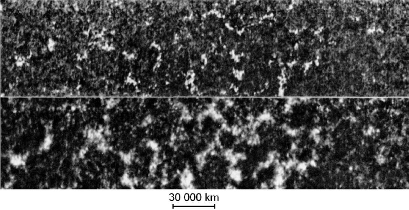
Abbildung 3.5: Simultaneous observations of the photospheric network in the CN band at 388 nm (top panel) and the chromospheric network in the Ca ii K line at 393 nm (bottom panel). The supergranular cells are visible due to bright network elements located at the cell boundaries and have a typical size of 30 Mm. From Liu & Sheeley (1971).

Dunn & Zirker (1973) observed the chromospheric network of the Sun with the 60-cm telescope of the Sacramento Peak Observatory using a narrowband (0.25 Å) H$\alpha$ filter. By tuning the filter from the core of the line to the wing, one looks at deeper and deeper layers of the solar atmosphere. Under excellent seeing conditions, Dunn & Zirker saw at 2 Å distance from the core of the H$\alpha$ line a pattern of grains roughly 0$\mbox{.}^{\prime\prime}$25 in size which were often interconnected into chains or crinkles. The grains and crinkles of this bright photospheric pattern named filigree were mostly located in the dark intergranular lanes.

Small bright features that are preferentially visible near the solar limb are called faculae (see Fig. 3.6) and were already observed by Chevalier (1914b). ten Bruggencate (1940) determined facular sizes of 1^′′-2^′′ and a mean lifetime of about one hour. Only Mehltretter (1974) was able to observe disk center faculae in his narrowband Ca ii K images (again with the 60-cm telescope of the Sacramento Peak Observatory). Under exceptionally good seeing conditions, he could resolve some of the faculae into several bright points (BPs) about 0$\mbox{.}^{\prime\prime}$25 in size. The BPs were clearly found in the dark intergranular lanes. Simultaneous observations in Ca ii K and H$\alpha$ revealed that the BPs and the filigree observed by Dunn & Zirker (1973) are the same phenomenon. From a comparison between his solar images and a Kitt Peak magnetogram, Mehltretter proposed magnetic flux concentrations in the photosphere to explain the facular points.

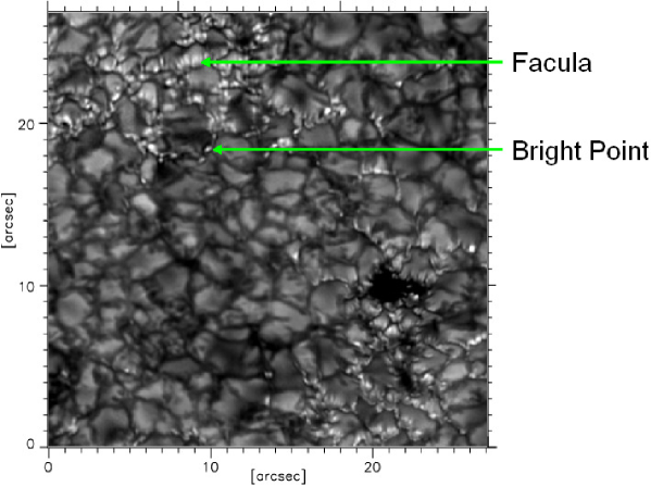
Abbildung 3.6: G-Band image showing various faculae and bright points as recorded at the 1m Swedish Solar Telescope in September 2004. Heliocentric angle was $\mu=\cos{\theta}=0.9$. The disk center direction is downwards. Adapted from Kobel et al. (2009).

Since the discovery of magnetic fields in sunspots (Hale, 1908), magnetic flux concentrations were also searched for outside spots and pores. Hale determined in his first successful measurements field strength in the range 200-300 G (Hale, 1922). The invention of the photoelectric magnetograph (Babcock, 1953) increased significantly the sensitivity of the magnetic field measurements and decreased the lower limit of the measurements to 1-200 G at a spatial resolution of 5^′′-20^′′. In the 1960s and beginning of the 1970s, the resolution of the magnetic field measurements could be partly improved to 1^′′, but the results were still contradictory. Field strengths of a few 100 G were found by Sheeley (1967); Grigorjev (1969); Abdusamatov & Krat (1969), while Beckers & Schröter (1968a) and Simon & Zirker (1974) reported kilo-Gauss fields. The limited spatial resolution of these measurements made it difficult to distinguish between strong field features that were much smaller than the resolution element and weak fields homogeneously distributed over the resolution element. Also dipole-like fields within the resolution element could not be detected since opposite polarities in the Stokes $V$ signal cancel each other.

The situation changed with the introduction of the line ratio method. Stenflo (1973) used the multi-channel magnetograph at the Kitt Peak Observatory to measure Stokes $I$ and $V$ profiles simultaneously for the two Fe i lines at 5247.0 Å ($g=2$) and 5250.2 Å ($g=3$). Both lines are formed in practically the same manner in the solar atmosphere and in the same atmospheric height range since they only differ in their effective Landé factors but have very similar properties otherwise (almost identical oscillator strengths and excitation potentials for the lower level, equal spin-orbit coupling energies for the lower and upper level), so that temperature and velocity in the solar atmosphere affect the lines identically. From the different Zeeman saturations of the two lines, Stenflo could retrieve field strengths, which were, for the first time, independent of the spatial resolution and of an underlying model. For network elements of the quiet Sun, he determined field strengths around 2000 G and characteristic sizes of the magnetic features in the range 100-300 km.

The kilo-Gauss fields found by Stenflo (1973) were confirmed several times by other authors. Harvey & Hall (1975) used the very Zeeman sensitive Fe i line at 15648 Å (see the quadratic $\lambda$ dependence in Eq. (2.6)) and found field strengths between 1500 G and 2000 G for magnetic elements outside active regions. Wiehr (1978) extended Stenflo’s line ratio method and used three spectral lines to determine field strengths of 1500-2200 G for Ca K BPs and H$\alpha$ faculae. Improvements in the spatial resolution made it possible to resolve BPs, so that the field strengths predicted by the line ratio method could be confirmed, for the first time by Keller (1992) with the help of speckle polarimetry and later by several authors (Berger et al., 2007; Ishikawa et al., 2007; Lagg et al., 2010).

The new insights gained in the 1970s and 1980s led to a picture of the formation and the structure of BPs that is largely still valid today: The energy produced by nuclear fusion processes in the core of the Sun is transported to the solar surface by radiation and in the outer zone by convection (see Fig. 2.1). The outer part of the convective zone is the place of the granulation cells, visible as the photospheric granulation pattern outside sunspots and pores. The electrical conductivity of the solar plasma is high so that the convective motions of the granulation transport the quasi frozen-in magnetic field lines from the inner parts of the granules to their outer regions, the intergranular lanes (Parker, 1963; Weiss, 1966; Tao et al., 1998). This flux expulsion process can concentrate the field in the intergranular lanes, in particular in the vertices of the granulation cells (Clark & Johnson, 1967), until the magnetic energy density is roughly equal to the kinetic energy density. The plasma trapped between the field lines cools by radiative heat losses at the solar surface (Parker, 1978; Grossmann-Doerth et al., 1998). The density increases and the plasma material flows down. Owing to the low density in higher layers, not enough material is replenished from above. Additionally, the nearly vertical magnetic field suppresses horizontal plasma motions. Thus, the intergranular regions of magnetic field are evacuated. The higher pressure outside these regions compresses the evacuated magnetic regions. This effect intensifies the inherent inhomogeneities and leads to a clustering of magnetic field lines so that thin flux tubes and elongated flux sheets are formed. Additionally, the interchange instability can cause a fragmentation of the elongated flux sheets into smaller flux structures. The evacuation of the flux tubes leads to a depression of the iso-$\tau$ planes, see Fig. 3.7. The radiative losses are in balance with the lateral inflow of heat through the walls of the depression. The inflowing heat makes the flux tubes hot and bright (Spruit, 1976) so that they can be observed as photospheric BPs (Deinzer et al., 1984). Near the solar limb, the line-of-sight is inclined relative to the flux tubes, so that the hot walls of the neighboring granules are observed as faculae (Berger et al., 2007). The flux tubes are mainly vertically oriented due to magnetic buoyancy (Schüssler, 1986). Because faculae are sometimes observed close to the disk center and BPs can also be detected near the limb, varying flux tube inclinations are under discussion (Kobel et al., 2009). However, the angle at which the hot walls of a flux tube become visible depends also on the thickness of the flux tube (see, e.g., Solanki et al., 2006). The external gas pressure, $p_{\mathrm{e}}$, is balanced by the pressure inside the flux tube that consists of the internal gas pressure, $p_{\mathrm{i}}$, and the magnetic pressure:

$$p_{\mathrm{e}}=p_{\mathrm{i}}+\frac{B^{2}}{2\mu_{0}}.$$ (3.1)

Pressure balance (Eq. 3.1) and magnetic flux conservation (Eq. 2.46) cause an expansion of the flux tube with decreasing external gas pressure, i.e. with increasing height.

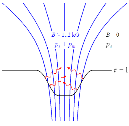
Abbildung 3.7: Sketch of a bright point as an expanding vertical flux tube. The magnetic field lines are drawn in blue color, the optical depth unity surface in black. The wavy red arrows illustrate the lateral inflow of heat through the walls of the flux tube.

In the quiet Sun, such magnetic elements are concentrated at the borders of the supergranulation cells and form the network. At sufficiently high spatial resolution, magnetic flux elements can also be observed in the interiors of supergranules where they are named internetwork elements. In active regions, outside spots and pores, the number density of magnetic elements is considerably higher than in the quiet Sun because of the higher mean flux density in active regions (see chapter 9). A large fraction of the intergranular lanes is filled with flux tubes or sheets and hence plage regions are formed.

Since Muller & Roudier (1984), photospheric BPs are preferentially observed in Fraunhofer’s G band, a spectral range between 4295 Å and 4315 Å which is dominated by lines of the CH molecule. The degree of dissociation of this molecule depends strongly on temperature and hence causes high contrasts for the G band BPs (Rutten, 1999; Steiner et al., 2001; Schüssler et al., 2003). The same is true for other molecular bands, e.g. the violet CN band at 3880 Å. Magnetograph observations are typically done in the green and red spectral range. In contrast to this, imaging in the blue G band has some advantages: a) shorter wavelength and hence lower diffraction limit, b) lower integration times (broad wavelength band) and hence less degradation due to seeing effects, c) higher cadences, and most notably d) fewer instrumental requirements. Almost all G band observations have a higher spatial resolution than comparable magnetographic observations, so that the field of proxy-magnetometry was established, a technique to identify magnetic features owing to their locally enhanced intensity. The usefulness of proxy-magnetometry was confirmed by comparisons between simultaneous recordings of G band images and magnetograms (Berger & Title, 2001; Berger et al., 2007). Further confirmation came from MHD simulations which revealed BPs as radiative signatures of magnetic flux concentrations (Schüssler et al., 2003; Shelyag et al., 2004). The converse argument is not valid since magnetic field concentrations do not always coincide with an enhanced intensity. Very small magnetic elements can appear dark because their contrast is smeared over the darker intergranular lanes (Title & Berger, 1996). Somewhat larger magnetic features display neutral contrast or are darker than the mean quiet Sun (Spruit & Zwaan, 1981; Grossmann-Doerth et al., 1994). Ishikawa et al. (2007) studied a plage region and reported on extended areas with high magnetic flux (magnetic islands). BPs are preferentially located near the boundary of such islands.

The long history of BP studies is continued in chapter 8 by analyzing quiet-Sun regions at disk center observed by the balloon-borne 1-m telescope Sunrise. Broadband observations in various spectral ranges of the near UV were achieved simultaneously with full Stokes measurements of a magnetograph operating in the visible spectral range. For the first time, BPs could be spatially resolved for wavelengths below 350 nm. Brightness, velocity, and polarization degree of a few hundred BPs are analyzed. Sunrise observations are compared with three-dimensional state-of-the-art MHD simulations of several mean flux densities in chapter 9. Synthetic Stokes profiles are calculated from the MHD data by solving the Unno-Rachkovsky equations numerically, including for the first time for the OH band at 312 nm. While the comparison between observation and simulation of existing studies mainly concentrated on intensity histograms, chapter 9 considers many more observational quantities (intensity at multiple wavelengths, LOS velocity, spectral line width, and polarization degree).

Kapitel 4 Instrumentation

The core of this thesis are the five studies that constitute the chapters 5-9. The used observational data were recorded with three different telescopes: Observations with the ground-based Swedish-Solar-Telescope (SST) are analyzed in chapter 5. Chapters 6 and 7 utilize recordings of the space-borne Solar Optical Telescope (SOT) onboard the Hinode satellite. Data of the balloon-borne observatory Sunrise are studied in the chapters 8 and 9.

This chapter describes the used telescopes, optical setups, and instrumentation in more detail than possible in a scientific publication. I spent a large part of my Ph.D. time with technical work for the Sunrise observatory. Some examples are the entire software development of the Sunrise Filter Imager (SuFI), the reduction of the SuFI data after the flight, the development of fundamental parts of the software for the Instrument Control Unit (ICU), and the conceptual design of the Data Storage Subsystem (DSS). For this reason, in the following the Sunrise topic is considerably more pronounced than the SST and SOT topics.

4.1 The Swedish Solar Telescope

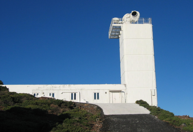
Abbildung 4.1: The Swedish Solar Telescope on the Canary Island La Palma.

The SST is a ground-based telescope of the 1-m class (Scharmer et al., 2002, 2003a). It is located on the Canary Island La Palma (Spain), close to the peak of the Roque de los Muchachos (see Fig. 4.1). The low temperature variations of the Atlantic Ocean and the low air pressure at an altitude of 2360 m above sea level make this one of the most suitable places for solar observations worldwide. The telescope is run by the Institute for Solar Physics of the Royal Swedish Academy of Sciences in Stockholm. With a clear aperture of 96 cm, the SST was put into operation on 2002 May 21 and replaced the 47.5 cm Swedish Vacuum Solar Telescope (SVST) that was operated at the same location from 1985 to 2000 (Scharmer et al., 1985).

Most of the modern solar telescopes are reflectors having an on-axis design (e.g. the Sunrise telescope described in section 4.3), i.e. the primary mirror has a central hole through which the light beam passes. The hole as well as the spiders needed to mount the secondary mirror cause an obscuration which lowers the contrast of the images significantly. This constructional shortcoming was avoided in the SST design by using a 1 m primary lens. The lens is also used as the entrance window to the vacuum tower in which the sunlight is re-directed with the help of two plane mirrors to the optics laboratory located in the basement of the telescope building. The vacuum prevents the deformation of the wavefront by air turbulence inside the tower. The SST has an alt-azimuth mount. Chromatic aberrations caused by the primary lens are compensated by a Schupmann corrector (Schupmann, 1899). The focal length of the telescope is 20.3 m (determined at a wavelength of 460 nm).

For the study in chapter 5, the setup shown in Fig. 4.2 was used by Vasily Zakharov for observations of the active region NOAA 10667 on 2004 September 7. The light leaves the vacuum tank in the optics laboratory, is reflected by the tip/tilt and deformable mirror, passes the reimaging lens and the field stop, and hits the first beam-splitter BS1. Wavelengths shorter than 500 nm can pass the beam-splitter (blue beam) but longer ones are reflected (red beam). 90% of the red light can pass a second beam-splitter BS2 and hit the TiO 7057 Å interference filter having a width of 7.1 Å. The following Kodak Megaplus CCD camera (9 $\mu$m pixel size) acquired the data of chapter 5. The remaining 10% of the red light are reflected by BS2 to the adaptive optics (AO) of the SST (Scharmer et al., 2003b). BS3 divides the beam once more between correlation tracker camera and wavefront sensor camera. The correlation tracker controls the two axes of the tip/tilt mirror and hence compensates for the rotation of the Sun around its own poles as well as for smaller image shifts due to turbulence in the terrestrial atmosphere, so that the observed solar object is at a fixed position within the field of view.

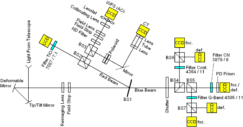
Abbildung 4.2: Optical setup used on September 7, 2004 for imaging in the titanium oxide band head with the Swedish Solar Telescope.

The Shack-Hartmann wavefront sensor (Hartmann, 1900; Shack & Platt, 1971) provides the control signals for the deformable mirror which compensates for higher order aberrations. Fig. 4.3 demonstrates the main principle. The heart of the Shack-Hartmann wavefront sensor at the SST is a hexagonal microlens array (called lenslet array) with 37 elements placed in a conjugate pupil plane. Each microlens forms an image of the source. The shifts of the images among each other are determined via correlation functions and yield the gradients of the wavefront deformations. The deformable mirror is also placed in a conjugate pupil plane and its 37 electrodes are now controlled such that the wavefront deformations are compensated as well as possible.

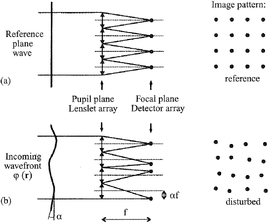
Abbildung 4.3: Principle of the Shack-Hartmann wavefront sensor. The example of a plane wave is given in panel (a), a disturbed incoming wavefront in panel (b). From Roddier (1999).

The five CCD cameras of the blue beam are all synchronized by an external shutter (for exactly simultaneous observations). A phase diversity configuration (see section 4.3.5) in each case records data for the violet CN band, the G band, and the blue continuum. The data of the blue beam are analyzed by Zakharov (2006) and Kobel et al. (2009), but are ignored in this thesis. Therefore we skip details.

As a final remark it is mentioned, that the active region NOAA 10667 investigated in chapter 5 was also observed at the Italian-French Themis observatory. Spectropolarimetric observations were done simultaneously in the six wavelength ranges 5139-5145 Å, 5197-5203 Å, 5247-5253 Å, 5872-5879 Å, 6705-6709 Å, and 7053-7059 Å and first results are published in Arnaud et al. (2006) and Wenzel et al. (2010). In spite of a similar aperture of 90 cm, the effectively reached spatial resolution of the Themis data is significantly lower than for the SST data due to the higher optical performance of the SST.

4.2 The spectropolarimeter aboard the Hinode satellite

The Hinode satellite (former name: Solar-B) is a space-borne solar observatory which was developed under the leadership of the Japanese space agency JAXA and is operated in cooperation with American and European institutes (Kosugi et al., 2007). Hinode was launched on 2006 September 23 at 06:36 (JST) from the Kagoshima space center with a Japanese M-V rocket. At an altitude of about 600 km, the Hinode satellite orbits the Earth and observes the Sun with three telescopes, see Fig.4.4. Corona and transition region are observed by the X-ray telescope (XRT) and the EUV imaging spectrometer (EIS). Photosphere and chromosphere are the target of the Solar Optical Telescope (SOT).

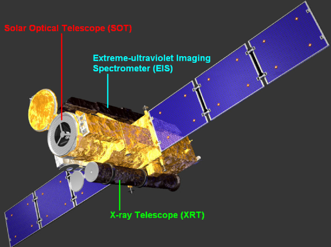
Abbildung 4.4: The Hinode satellite carrying the Solar Optical Telescope. Adapted from Shimizu (2008).

The SOT is a Gregory-type on-axis telescope (Suematsu et al., 2008; Tsuneta et al., 2008) whose design is schematically drawn in Fig. 4.5. The aperture of the SOT is 50 cm, the effective focal length is 4527 mm. The sunlight is reflected by the primary and secondary mirror, passes the hole in the primary mirror, and hits the Collimator Lens Unit (CLU). The collimated beam passes the Polarization Modulator Unit (PMU, a retarder plate rotating with 5/8 Hz), is reflected by the tip/tilt mirror, and enters the beam distributor which then distributes the light to the Correlation Tracker (CT, Shimizu et al., 2008) and to the three scientific instruments, NFI, BFI, and SP. While BFI (Broadband Filter Imager) records purely photometric images for five photospheric (3883, 4305, 4504, 5550, and 6684 Å) and one chromospheric (3968 Å) wavelength range, the NFI (Narrowband Filter Imager) and SP (Spectropolarimeter) are two vector magnetographs. NFI allows the observation of two-dimensional Stokes images with a high cadence but only moderate spectral resolution of 90 mÅ (at 6300 Å) with the help of a tunable Lyot filter. For photospheric magnetograms, the Fe i lines at 5247.1, 5250.2, 5250.6, 6301.5, 6302.5 Å or the Ti i 6303.8 Å line can be scanned. Chromospheric magnetograms and Dopplergrams can be retrieved from scans of the Na i 5896 Å or Mg i 5172.7 Å line, photospheric Dopplergrams from the Fe i 5576 Å line, and finally, the chromospheric H$\alpha$ 6563 Å line can be scanned. Since chapters 6 and 7 only uses data of the spectropolarimeter, no further details about the broad- and narrowband imagers are given here. The interested reader is referred to Hurlburt et al. (2009).

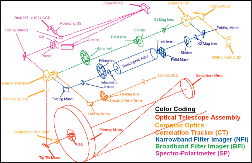
Abbildung 4.5: Optical schematic of the Solar Optical Telescope (SOT) onboard the Hinode satellite and its focal plane instrumentation. From Hurlburt et al. (2009).

The SP is a slit spectrograph in Littrow configuration for the wavelength range 6300.8-6303.2 Å with a high spectral resolution of 30 mÅ at a low cadence (Lites et al., 2001). An Echelle grating having 79 grooves/mm is used as the dispersive element and is operated in the 36th order. A polarizing beam-splitter serves as analyzer and creates two orthogonal linearly polarized states, each of them imaged at one half of the CCD. The dual-beam configuration allows a considerable reduction of cross talks which can occur by residual motions or vibrations of the satellite (Lites, 1987; Skumanich et al., 1997). The CCD camera is continuously exposed and read out synchronously with the PMU: 16 spectra are recorded per PMU revolution. A prototype of the SP was installed at the Dunn Solar Telescope as the Diffraction Limited Spectro Polarimeter (DLSP) (Sigwarth et al., 2001).

The slit of the SP is 0$\mbox{.}^{\prime\prime}$16 wide and 164^′′ long and is oriented parallel to the solar North-South direction. It can be moved in the range of $\pm 164\mbox{${}^{\prime\prime}$}{}$ along the solar East-West direction with the help of a tiltable mirror, so that the solar surface can be scanned in a field of view of maximal $164\mbox{${}^{\prime\prime}$}{}\times 328\mbox{${}^{\prime\prime}$}{}$. SP has four operating modes: a normal map mode, a fast map mode, a dynamics mode, and a deep magnetogram mode. Only data of the normal map mode are studied in chapter 6, where the integration time per slit position is 4.8 s (3 revolutions of the modulator) and a polarimetric accuracy of $10^{-3}$ can be reached. The spatial sampling in the normal map mode is 0$\mbox{.}^{\prime\prime}$16 $\times$ 0$\mbox{.}^{\prime\prime}$16 and a 160^′′ wide map can be scanned in 83 min. The characteristics of the other three modes can be found in Hurlburt et al. (2009).

Compared to an imaging magnetograph like NFI, the big advantage of a slit spectrograph like SP is its high spectral resolution/sampling, so that a large number of wavelength points per spectral line is achieved. As demonstrated in chapters 6 and 7, this allows not only inversions that retrieve averaged physical quantities of the solar atmosphere, but also height-dependent inversions that can retrieve stratifications of the atmospheric quantities.

4.3 The balloon-borne observatory Sunrise

Sunrise is a balloon-borne solar observatory developed under the leadership of the Max-Planck-Institut für Sonnensystemforschung (MPS) in Lindau/Eichsfeld in cooperation with the Kiepenheuer-Institut für Sonnenphysik (KIS) in Freiburg/Breisgau, the High Altitude Observatory (HAO) in Boulder/Colorado, the Instituto de Astrofísica de Canarias (IAC) in La Laguna/Tenerife, the Instituto de Astrofísica de Andalucía (IAA) in Granada, the Instituto Nacional de Técnica Aerospacial (INTA) in Madrid, the Grupo de Astronomía y Ciencias del Espacio (GACE) in Valencia, and the Lockheed Martin Solar and Astrophysics Labotory (LMSAL) in Palo Alto/California.

The first scientific flight took place in June 2009 from Kiruna in Northern Sweden to Somerset Island in Northern Canada (Fig. 4.6). The distance of more than 4000 km was covered in 137 hours. The flight altitude of the balloon showed cyclical variations between day and night in the range 34-37 km. At a mean northern latitude of $\mathrm{71^{\circ}}$, the Sun was always above the horizon and could be observed 24 hours a day. Stratospheric balloon observations have two more advantages. 99% of the air mass are below the balloon, so that disturbing seeing effects known from ground-based observations practically do not exist. In addition, also wavelengths below 350 nm can be observed which is not possible from ground because of the absorption of the UV radiation in the terrestrial ozone layer. Sunrise was therefore designed for observations in the visible and near UV spectral range from the very first. The Post Focus Instrumentation (PFI) contains two scientific instruments: SuFI, a filter imager for the near UV and IMaX, an imaging magnetograph for the Fe i 5250.2 Å line in the visible (see below).

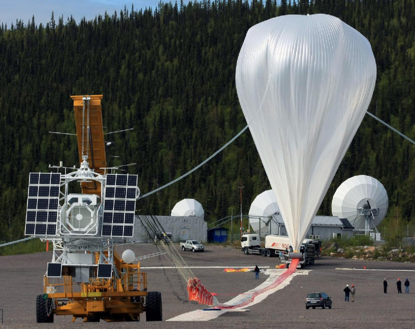
Abbildung 4.6: The Sunrise observatory a few minutes before the launch of the first science flight on 2009 June 8.

A complete description of Sunrise is not possible within the limits of this thesis. I only concentrate on those topics that were part of my work at MPS in the recent years. Extensive information about technical aspects of Sunrise can be found in Barthol et al. (2011) and the following Sunrise articles of same special issue of Solar Physics (Berkefeld et al., 2011; Gandorfer et al., 2011; Martínez Pillet et al., 2011). First scientific results of the 2009 flight were published as special issue of The Astrophysical Journal Letters, amongst others the study reproduced in this thesis as chapter 8. A good overview is given by the first article of the special issue, Solanki et al. (2010).

4.3.1 Telescope

Similar to Hinode/SOT, Sunrise is an on-axis Gregory-type telescope, whose optical configuration can be seen in Fig. 4.7. The parabolic primary mirror (M1) has a focal length of 2.42 m and a diameter of 1 m and makes Sunrise the largest solar observatory that ever left Earth’s surface. A Heat Rejection Wedge (HRW) is placed in the primary focus (F1) and reflects 99% of the unwanted heat load into cold space. Only the light passing a 2.8-mm wide hole in the HRW can hit the 24.5 cm elliptical secondary mirror (M2). The effective focal length of the Gregory telescope is 24.2 m. The two plane mirrors M3 and M4 direct the light into the PFI placed on top of the telescope. The mirrors M2, M3, and M4 can be moved via mechanisms, so that the telescope can be readjusted in flight, in particular it can be refocussed.

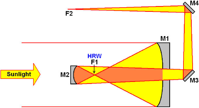
Abbildung 4.7: Optical configuration of the Gregory telescope of Sunrise.

4.3.2 Light distribution and image stabilization

The Image Stabilization and Light Distribution (ISLiD) unit distributes the light with the help of dichroic beam-splitters, according to wavelength, to the two scientific instruments SuFI (200-400 nm) and IMaX (525 nm) as well as to the Correlating Wavefront Sensor (CWS, 500 nm), so that the three camera-based instruments can be operated simultaneously. ISLiD has to preserve the diffraction-limited performance and the polarization information of the light (only important for IMaX). A magnifying optical system reimages the secondary focus (F2) onto SuFI science focus, so that the effective focal length of SuFI is 121 m.

A motor-driven filter wheel placed in the secondary focus has a closed position for taking dark current measurements, a pinhole position for checking the alignment between the three camera-based systems and for internal calibrations of the CWS, and an open field position for the normal solar observations. The CWS is a six-element Shack-Hartmann wavefront sensor, which compensates for image motions in the range 1-30 Hz by controlling a fast tip/tilt mirror ($\pm$ 46^′′ range) and corrects for defocus and coma by moving the three axes of M2. More details about the CWS can be found in Berkefeld et al. (2011), details about ISLiD in Gandorfer et al. (2011).

4.3.3 Software architecture

The challenge of designing the hardware and software for the Sunrise observatory is posed by the science requirements (Schüssler, 2004) which had to be reconciled with the technical feasibilities, in particular with respect to mass, power consumption, and telemetry bandwidth. A substantial design driver was the fact, that the data rate provided by IMaX and SuFI in the observing modes (5-7 MBytes/s) are orders of magnitudes higher than the available telemetry downlink rate of 6 kBit/s (gross). The following conceptual design was chosen: Every camera-based instrument is equipped with an embedded PC acquiring and pre-processing the camera data as well as controlling the mechanisms. Via a 100 MBit Ethernet, each instrumental computer is connected with the Instrument Control Unit (ICU), a central computer also located in the gondola and connected to the ground station via telemetry channels, see Fig. 4.8. Each instrument transfers its image and housekeeping data to the ICU, which stores all data on a central Data Storage Subsystem (DSS) and, if telemetry bandwidth is available, sends important parts of the data to the ground station.

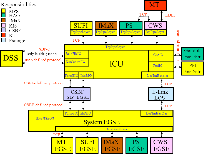
Abbildung 4.8: Flight configuration of the Sunrise software architecture. From Riethmüller (2006a).

The ground station receives the telemetry data centrally via the System EGSE (Electrical Ground Support Equipment). The most important software component of the System EGSE is a configurable ground support software named GSEOS, which was developed by the Institut für Datentechnik und Kommunikationsnetze (IDA) in Braunschweig (Reiche et al., 2009). System relevant housekeeping values are displayed on various screens and a color-code indicates out-of-range values. The System EGSE also provides the possibility of transferring tele-commands from ground to the ICU. Instrument-specific housekeeping displays and commanding capabilities are provided by separate Instrument EGSEs which are connected to the DataDistributor software via a TCP socket interface (Riethmüller, 2006b). The DataDistributor was developed by MPS and establishes a data connection to the GSEOS running on the System EGSE (Riethmüller, 2006c). Since GSEOS is specialized in processing and displaying housekeeping data but is not optimized for the processing of large amounts of image data, an additional Qt-based SuFI EGSE software can be connected to the DataDistributor which is aimed at the analysis and processing of solar images.

The most time-critical parts of the ICU software due to high data rates are the receiving of image data send by the instruments, the RAID level 5 coding in software, and the data saving on the DSS. Additionally, the ICU has to perform various I/O tasks having uncritical data rates, e.g. sending of telemetry data, receiving and execution of tele-commands, operating the gondola and PFI power distribution units, acquisition of housekeeping data via the Sensor Interface Board (von der Wall, 2005), etc. The execution of one service must not block the software and hence inhibit the completion of other services. At the same time the software has to be maintainable and upgradeable. Such requirements can only be realized by a concurrent programming model.

Classical operating systems like Microsoft Windows or Linux provide concurrency in the form of threads and processes. In the case of the ICU software, the telemetry services were put in separate processes in order to decouple the telemetry processing from other software parts as completely as possible, so that a possible fatal software error does not fully block the tele-commanding capabilities of the entire system. The remaining tasks are distributed over several threads of a single process in order to guarantee a maximal data exchange rate between the concurrent branches of the software.

A distributed multi-threaded software is error-prone and difficult to debug and hence a challenge even for software engineers with many years of experience (think of deadlocks, race conditions, thread synchronization, etc.). Nevertheless, a notedly reliable software had to be developed which can run without errors or interruptions for at least six days. The following software design tries to fulfill these requirements:

1) From the software’s point of view the interface between instrument and ICU is placed inside the instrument software and not, as usual, at the Ethernet hardware. Since a symmetrical programming style for the data sending and receiving software parts enables the lower transport layers of the software (named TcpPipeLayer in Fig. 4.8) to be identical for the ICU and the instruments, the know-how developed at MPS could be made accessible to the partner institutes in the form of software libraries. This reduced their development effort and limited significantly the effort needed to optimize the performance of the data transfer, because an instrument simulator provided as part of the MPS software package could be used as benchmark and as application example of the libraries.

Taking these advantages brought up two difficulties. On the one hand, the instruments are operated with different operating system families and hardware architectures. This requires a careful treatment of byte order issues when transferring multi-byte numbers and it excludes the usage of non-portable operating system functions. The native Application Programming Interfaces (APIs) for the socket (network) interface and thread programming are, however, not portable between different operating system families (Stevens, 1997; Schmidt et al., 2000). On the other hand, the TcpPipeLayer could not be designed with an object-oriented interface (which would have had some advantages, e.g. type safety), because not all instrument suppliers used the object-oriented programming language C++.

2) Portability between different platforms as well as robustness and reliability of the software were reached by the forceful usage of the Adaptive Communication Environment (ACE) library (Schmidt & Huston, 2001, 2002; Huston et al., 2003) which has been used very successfully on many platforms for more than two decades. By the application of design patterns (Gamma et al., 2005) like Wrapper Facade, Thread-Safe Interface, Acceptor/Connector, etc. (Rising, 2000; Schmidt et al., 2000), non-portable data structures and APIs are encapsulated and hence object-oriented and type-safe class interfaces are provided by the creation of reasonable abstractions.

The heart of the TcpPipeLayer is a Thread Pool Reactor (Schmidt et al., 2000; Schmidt & Huston, 2002), which is preferentially responsible for the data receiving from the socket interface. A pool of 10 threads makes the TcpPipeLayer responsive at all times, even if the ICU is receiving image and housekeeping data simultaneously from multiple instruments. The data sending is realized with synchronous function calls.

Access to a serial interface is mostly implemented in a separate thread which processes a queue containing all write requests to the interface. Reading from the serial interface is done with synchronous function calls according to a strict master-slave principle, i.e. data are only expected to be read after a previous write access.

3) An easy expandability of the software is reached by the forceful use of interface classes (Meyers, 1995, 1997), which makes the application of a software component independent of its implementation. Fig. 4.9 shows as an example the interface class ISaveTo, which uses the ICU to save data received from an instrument. The ICU flight software is identical with the ICU simulator (SrIcuSim) and differs only in the usage of different command line options. The ICU software contains always a SaveToDss object, which stores images (Im) and housekeeping data (Hk) either on the DSS in a RAID level 5 coded format (flight version, command line option -raid) or on a hard drive in an uncoded format (important for the test and calibration phase, no command line option) or the data are not stored at all (important for measurements of the data rate, command line option -nodiscio). Housekeeping data and thumbnails (Th, small images suitable for transferring to the ground station) can be optionally send to the ground station via a telemetry channel (command line option -usetm) or to the DataDistributor (command line option -useddb, important for the software development phase, see also Riethmüller, 2006a). An extension by a fourth alternative of data saving is easily possible because the ICU software knows nothing about the concrete implementation but only calls member functions of the ISaveTo interface.

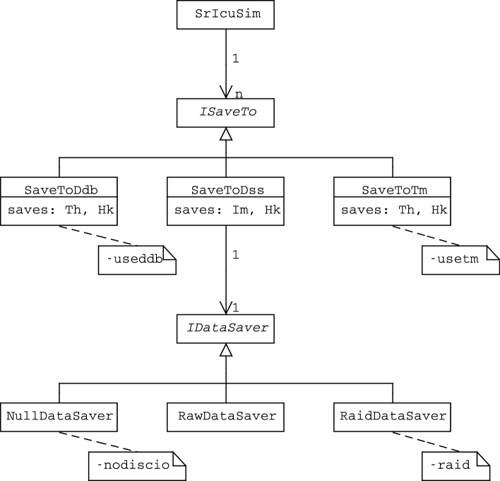
Abbildung 4.9: Class diagram showing the various methods of data saving implemented in the ICU software.

4) Run-time errors are difficult to identify, in particular in distributed concurrent software projects. Therefor multiple platform-independent tools were developed that are specialized in the detection of some typical run-time problems.

Data saving of large amounts of scientific data on the DSS can only be implemented efficiently in software if possible bottlenecks can be detected quickly and reliably, e.g. with the help of a profiler. A profiler tells the software developer which functions of a running software are called how many times and how much CPU time they spend. In a multi-threaded software, the output of a profiler should be separated by threads. If the software runs into a deadlock, the problem can be mostly identified by outputting the call stack of the software, again separated by threads. Call stack logging and profiling are realized by the technique of Method Call Interception (MCI, Sayfan, 2005) which is explained below.

As a start, a tool named InsertMci was developed which is called as a pre-built command for each source file (similar to the C/C++ pre-processor tool). InsertMci inserts an additional source code line in the format ’MCI(ClassName,MemberName);’ at the entry point of each member function. The name of the class and the member function are previously determined by the InsertMci tool. At run-time, each entry point of a member function calls the constructor of an MCI object, the corresponding destructor is called when the member function is left. If the profiler was registered at the MCI object, the time elapsed between constructor and destructor call can be measured and the call counter can be incremented. In the case of the call stack logger, class and member function name are pushed onto a stack in the constructor and removed from the stack in the destructor. Since the execution of the MCI constructors and destructors also need resources, MCI can be completely ignored via a compiler option. There is also the possibility to switch off MCI only for some time-critical member functions. The output of a call stack or profile can be triggered from outside at any time by running a further small tool that plays the role of a client and establishes a socket connection to the ICU software. Call stack logger and profiler are part of the ICU software and contain a server component which responds to the client request by outputting the call stack or profile, respectively.

Finally, the memory checker tool is mentioned which can detect the following memory management problems: a) memory leaks, i.e. memory was allocated but never released, b) multiple-releases of memory, and c) programming errors of the form new/delete[] or new[]/delete. Note that neither memory checker nor MCI functions are allowed to use the ACE library, otherwise a run-time analysis of the initialization and finalization of ACE, including the Singletons managed by the ACE object manager, would not be possible.

5) Finally, the robustness of the software was improved by the use of the C++ standard library with its highly efficient container classes and algorithms (Kuhlins & Schader, 2005) as well as by ensuring const correctness (Meyers, 1997), i.e. whenever an object should not be modified, this fact has to be communicated to the compiler and to other software engineers by using the C++ key word “const”.

4.3.4 Data storage

The Data Storage Subsystem (DSS) is an onboard mass memory to store the housekeeping and scientific image data persistently. The DSS consists of 48 hard disks (2.5^′′) having a capacity of 100 GBytes each. To save electrical power, only four of the 48 disks are switched on. One of the four disks stores the parity bits of the other three disks (RAID level 5), so that the data can be completely recovered in the case of a single failure. Hence, the net capacity of the DSS is 3.6 TBytes. The switch over from one four-disk-chain to the next requires a hot-pluggable interface with a bandwidth of more than 100 MBit/s, e.g. USB or IEEE 1394. It was decided to use the IEEE 1394 interface because the operation of multiple hard disks using this interface does not require an additional hub (see also Riethmüller, 2006d). Housekeeping data and commands are transferred between ICU and DSS via an RS422 interface (Tomasch, 2008).

The used hard disks need certain air pressure and humidity levels that cannot be found in the stratosphere. Therefore, a pressurized vessel was used, where the 48 disks were distributed over two vessels for redundancy reasons. The vessels are mounted at a position within the gondola structure that is as safe as possible during the landing, see Fig. 4.10.

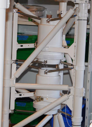
Abbildung 4.10: The 2 pressurized vessels of the Data Storage Subsystem.

4.3.5 Filter Imager

The Sunrise Filter Imager (SuFI) is a phase diversity assisted broadband imager for the near UV which takes advantage of the observing conditions in the stratosphere. SuFI samples the solar photosphere and chromosphere in five different wavelength ranges. The shortest wavelength, 214 nm, allows investigations of the upper photosphere at a theoretical diffraction limit of 0$\mbox{.}^{\prime\prime}$05, corresponding to 40 km on the solar surface. Imaging the quiet photosphere with the 312 nm or 388 nm filter provides intensity images that show high contrasts for bright points because of the large number of molecular lines in these spectral ranges. In contrast, the 300 nm filter allows photospheric observation without important molecular contributions. The emission peaks on both sides of the core of the Ca ii H line at 397 nm are thermometers measuring the temperature structure of the chromosphere.

SuFI consists of a filter wheel for the selection of the wavelength range, a shutter to limit the exposure time, a Mechanism Controller (MC) for the control of the filter wheel and the shutter, a UV sensitive camera, and an Electronics Unit (EU) which contains an embedded PC as instrument computer.

Mechanisms

The exposure time of the images acquired by SuFI is controlled by a mechanical shutter (Müller, 2007). A commercial two-blade shutter produced by the Japanese company Nikon is used in combination with a cock mechanism developed at MPS. The two blades move time-delayed to each other in the same direction and allow exposures of the SuFI camera with a precision better than 0.1 ms which makes very short exposures possible.

The selection of the wavelength is done with the help of a filter wheel having six filter positions. The change between two neighboring positions lasts about 1 s which possibly influences the maximal reachable cadence of multiple-wavelength observing modes. The Planck curve decreases drastically for short wavelengths so that unwanted leakage contributions from higher wavelength ranges can only be avoided by the use of two filters. The two filters are mounted in two separate filter wheels which are parallel to each other and rotate in opposite directions to minimize the torsional moment induced into the SuFI structure. Only the highest wavelength requires only a single filter. The filters are assigned to the filter wheel positions such that quick changes between photospheric and chromospheric observations are possible (Riethmüller, 2008a). Because SuFI only observes in five wavelength ranges, the sixth filter wheel position can be used for a lens to image the entrance pupil which is beneficial during the integration of SuFI into the PFI structure. Table 4.1 lists all filters with their nominal central wavelength, the width of the filter, the filter wheel position, and the typical exposure time.

Tabelle 4.1: Assignment of the 6 filter wheel positions of SuFI.

Pos.	$\lambda$	FWHM	# Filters	Exp. Time	Description
	(nm)	(nm)		(ms)
O	388	O.8	2	1OO	CN band head, photosphere
1	396.8	O.18	1	1OOO	Ca ii H, chromosphere
2	3OO	5	2	3OO	continuum, photosphere
3	312	1.2	2	2OO	part of the OH band, photosphere
4	214	1O	2	3OOOO	upper photosphere
5	lens+ND				pupil images during integration

Shutter and filter wheel are controlled by the SuFI Mechanism Controller which is commanded by the SuFI Electronics Unit via a serial RS422 interface (see Müller, 2009). Furthermore, the SuFI Mechanism Controller switches the power of the camera and the filter wheel, controls the two fans inside the pressurized camera electronics box, and controls the external trigger signal of the camera.

Phase diversity prism

Wavefront deformations can be determined by the method of Phase Diversity (PD) in which a target is simultaneously imaged twice with a well-known defocus between the two images (Gonsalves & Chidlaw, 1979; Paxman et al., 1992; Hirzberger et al., 2011). The true object as well as the aberrations can be retrieved from such observations. SuFI was designed as a PD imager in order to have the possibility of correcting the observations for residual aberrations that can be caused by thermoelastic deformations of the telescope and PFI structure. A PD image doubler (Grauf, 2007) is mounted directly in front of the camera head, so that each target is imaged twice. The left half image is nominally focussed, the right half image is defocussed by 28 mm which corresponds to one wave at 214 nm. This reduces indeed the effective field of view (which is now rectangular) but allows an optimal reconstruction of the images within the post-flight data reduction process.

Camera

The core of the SuFI instrument is a BioXight BV20CCD camera of the company PixelVision of Oregon, Inc., in which a Charged Coupled Device (CCD) sensor of the company Scientific Imaging Technologies, Inc. (SITe) of the type S100AB-04 is used. This detector is a back illuminated $2\rm{K}\times 2\rm{K}$ CCD with a pixel size of $12\leavevmode\nobreak\ \rm{\mu m}\times 12\leavevmode\nobreak\ \rm{\mu m}$, four read-out channels, 100% filling factor, and a dark current of only 1.82 electrons/pixel/sec at 240 K CCD temperature. The CCD sensor is cooled by a Peltier element whose hot side is in turn cooled by a liquid cooling system. The camera electronics digitizes the analog CCD signals to 14 bit and the digital data are transferred to a PCI interface card of type Lion2 inserted in the SuFI computer. Quantum efficiencies of more than 50% (see Fig. 4.11) and a maximal frame rate of 2.64 frames per second fulfill the scientific requirements (Schüssler, 2004) and make this CCD a nearly ideal sensor for SuFI.

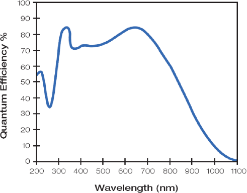
Abbildung 4.11: Quantum efficiency of the SITe back illuminated CCD S100AB-04 used in the Sunrise filter imager. Adapted from the SITe S100A data sheet.

The commercial camera had to be modified for utilization in SuFI. Since the Peltier element can only provide a temperature difference of at most 25 K, the element’s hot side was connected to a radiator via heat pipes and the camera head was separated from the camera electronics in order to allow two different temperature levels for the two subsystems. The multitude of difficult to access hot spot components in the camera electronics made a possible alteration of the electronics to vacuum suitability too risky, so that a pressurized vessel was used to house the camera electronics. Two fans control the air circulation inside the vessel which is connected to a second radiator. The two radiators emit the heat excess into cold space. During the flight, the CCD was cooled by the Peltier element to 268 K which led to the optimal compromise between dark current, noise, and power consumption as determined by extensive dark current measurements at different CCD temperatures (Riethmüller, 2008b).

Problems with the vacuum feedthroughs of the original fiber optic cables between camera electronics and SuFI Electronics Unit led to an alteration to differential signaling via copper cables. Finally, a SuFI power supply had to be developed at MPS for the 28 V primary power of the gondola.

Electronics unit

The SuFI Electronics Unit controls all components of the SuFI instrument and connects the SuFI camera with the ICU. Camera data are received by the EU, pre-processed, and transferred to the ICU. Additionally, commands are received from the ICU and executed, e.g. to move the SuFI mechanisms.

The hermetically sealed EU box contains an IBM compatible single board computer, the PCI camera interface card, and a Sensor Interface Board connected to the single board computer via a serial RS232 interface (Dackweiler & Bittorf, 2006). Additionally, interfaces for external components are provided: a 100 MBit Ethernet interface for connecting the ICU and a serial RS422 interface for connecting the SuFI MC.

The Sensor Interface Board developed by the company DSI is identical to the board used by the ICU, it controls the fans inside the pressurized EU box and it acquires several housekeeping values (von der Wall, 2005). The single board computer is an AMPRO LittleBoard 800 (AMPRO, 2005) which possesses an Intel 1.4 GHz LV Pentium M 738 processor, 1 GB RAM, and a 4 GB compact flash disk.

Flight software

The main task of the SuFI software is the execution of observing programs according to the observing plan defined by the Sunrise team (Schüssler et al., 2009). Observing programs are sent from the ICU to SuFI and require a flexible use of the instrument, i.e. all use cases mentioned in the following list have to be covered:

• SuFI shall acquire time series at fixed wavelengths in order to study highly dynamical solar surface phenomena at the maximum cadence.

• SuFI shall changes between a photospheric and a chromospheric wavelength as fast as possible.

• SuFI shall cycle through all five wavelengths in order to sample all available atmospheric heights.

• SuFI shall finish the observation after the acquisition of a given number of images.

• SuFI shall finish the observation if a given time is elapsed.

• SuFI shall observe a given selection of wavelengths for a given period of time, afterwards a cycle through all five wavelengths shall be done once and the entire procedure shall be then repeated.

The implementation of these use cases in software was carried out using the proven methods already mentioned in the context of the ICU software (see section 4.3.3), i.e. the use of:

• the TcpPipeLayer for the communication between SuFI and ICU,

• the ACE library for multi-threading, thread synchronization, error message handling, etc.,

• interface classes,

• design patterns,

• memory checker, call stack logger, and profiler for analyzing the run-time behavior of the software.

An observing program consists of a sequence of commands which are serially executed by the SuFI software. In the normal case, the ICU sends such command sequences at a certain point in time (timestamp) according to the SuFI timeline which is stored on the ICU. It is also possible to send manual commands from the ground to SuFI in order to manipulate or cancel running observing programs. For such manipulation or cancelation commands, a second logical way of commanding has to exist because the first way is already blocked by the execution of the observing program. Therefore, low- and high-priority commands are introduced. Low-priority commands can be both, very simple commands or more complex commands needing a long execution time, e.g. the acquisition of an image series. High-priority commands must be simple and hence require a short execution time, e.g. the cancelation of an observing program ahead of time, setting a flag, or modifying a parameter. For each command it has to be known a priori whether it is a simple or a complex command.

The concurrency model of the SuFI software is displayed in Fig. 4.12. The entry point of the software is the construction of the application object of type SufiInst by the main thread (central part of Fig. 4.12). The main thread initializes the TcpPipeLayer with its pool of reactor threads. One of the reactor threads receives low-priority commands from the ICU that are executed immediately in the case of a simple command or inserted into a command queue processed serially by the main thread in the case of a complex command. A second reactor thread receives high-priority commands from the ICU which are always executed immediately. A third reactor thread (HkSender) works as alarm handler and transfers a current snapshot of the housekeeping table to the ICU every 5 s. The ICU uses the regularly incoming Hk packets for a heartbeat monitoring of SuFI. If the Hk stream becomes silent for longer periods, the ICU power cycles SuFI.

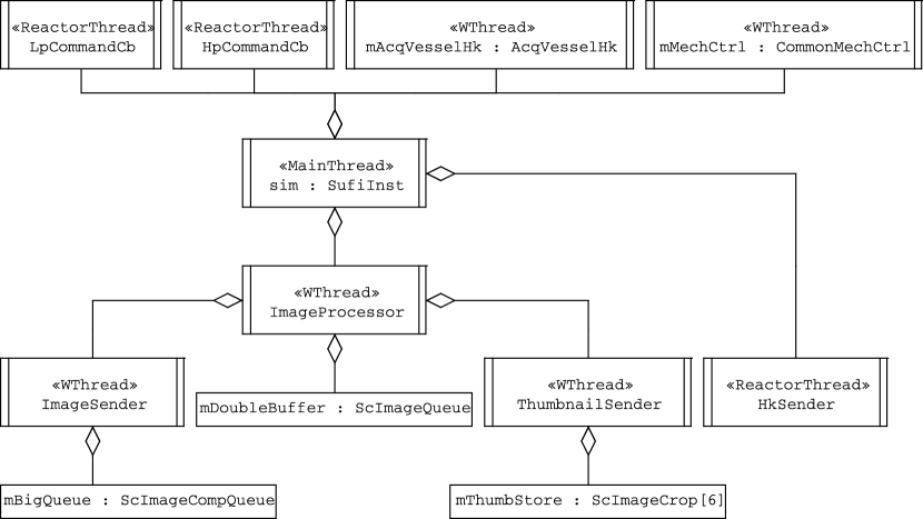
Abbildung 4.12: Concurrency model of the SuFI software. See main text for an explanation.

The main thread creates three further threads, the AcqVesselHk, the CommonMechCtrl, and the ImageProcessor thread. The processing of housekeeping requests from the Sensor Interface Board (e.g. pressure and temperature inside the pressurized EU vessel) using synchronous function calls lasts about 9 s and is hence implemented in a separate thread. This AcqVesselHk thread puts the housekeeping values into a global Hk table which always contains the latest Hk values of every SuFI component, e.g. the current filter position, which can be theoretically changed every second. The global Hk table decouples Hk acquisition and Hk transfer done by the HkSender thread. The CommonMechCtrl thread is an active base class which provides an interface to access the SuFI Mechanism Controller. There are two implementations of this interface. The first one simulates the MC hardware and is only needed during the software development phase for situations in which the real hardware is not available. During the flight, the second implementation is used which accesses the real MC. Again, MC commands are queued and housekeeping values of the MC are put into the global Hk table.

The ImageProcessor thread allows the compression of image data and the creation of thumbnails not only to be done in parallel to moving the filter wheel but also simultaneously with the transfer of data to the ICU. For this purpose, the ImageProcessor thread creates the ImageSender thread and the ThumbnailSender thread. The data flow of an image acquisition and its distribution over the various threads is shown in Fig. 4.13. The main thread initiates the read-out of the CCD into the free half of the double buffer for ScImage objects via the StartAcquisition action, where an ScImage object provides memory for a raw image and an image header. Then the main thread determines the current filter wheel position and exposure time from the MC in order to use these values together with other values from the global Hk table to fill the image header of the current ScImage object. In parallel to the CCD read-out, the filter wheel moves to the position of the next observation. If the CCD read-out is completed, the current half of the double buffer is tagged as ready for further processing.

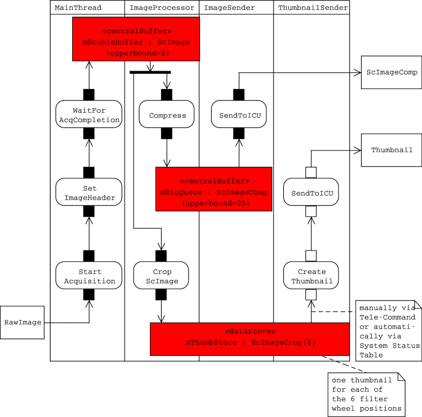
Abbildung 4.13: Overview of the image data flow of SuFI and its distribution over 4 threads to reach a maximum cadence.

While one half of the double buffer is being filled with image data, the previous image contained in the other half of the double buffer is processed by the ImageProcessor thread simultaneously. Such an ScImage object is compressed and inserted into the mBigQueue queue as ScImageComp object. mBigQueue can contain at most 25 images and must provide such a large amount of memory because sufficient buffer memory is needed for temporary interruptions of the data transfer to the ICU (e.g. during the switch over from one four-chain of the DSS to the next one). Whenever mBigQueue contains an image, the ImageSender thread tries to transfer the image to the ICU. If the system is overloaded, mBigQueue gets full and the oldest ScImageComp object is overwritten by a new one. Additionally, the ImageProcessor thread creates thumbnails from the double buffered ScImage objects. Because of the low telemetry rate, the amount of data required by a thumbnail needs to be considerably reduced by cropping (it is sufficient to down link the focussed half image), binning, bit truncation, and image compression. The parameters of the thumbnail creation are arbitrary within the valid ranges. For each filter wheel position, an up-to-date thumbnail is stored in mThumbStore as an ScImageCrop object. Thumbnails can be packetized and sent to the ICU by the ThumbnailSender thread, if the automatic thumbnail sending mode is switched on and/or a thumbnail is requested manually and if telemetry bandwidth is available for thumbnails. Whether this is the case is known from the System Status Table (Kolleck & Riethmüller, 2009) which is broadcast from the ICU to the instruments every 3 s and contains system information, e.g. the GPS position and altitude of the balloon, status of the aperture door, the F2 mechanism, and the mirrors M2, M3, M4, or the pointing quality of the gondola.

The acquisition of an image is repeated via the loop structure shown in Fig. 4.14. The serial processing of two inner loops within an outer loop guarantees that all the use cases mentioned above are covered, in particular the last mentioned use case with the highest requirements. The FilterLoop activity shown in Fig. 4.14 cycles through an array of 20 filter wheel positions that are commanded one after the other. A negative filter wheel position is thereby ignored, so that less than 20 positions can also be used in such a loop. After each image acquisition, a possible delay leads to the user-defined cadence. The positioning accuracy of the filter wheel is ensured to be high by not rotating the wheel always in one direction but such that after one wavelength cycle the wheel is rotated back to the first filter position. For a full five wavelengths cycle the filter positions can be commanded, e.g. in the order 0,1,2,3,4 (fast cycling, high return time) or in the order 0,2,4,3,1 (return time more uniformly distributed over several steps), just to mention two possibilities. A 16 bit integer value determines the completion of the FilterLoop activity. A positive value is interpreted as number of seconds, a negative value as number of cycles.

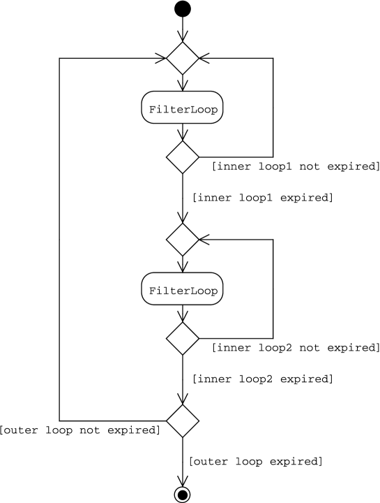
Abbildung 4.14: Activity diagram visualizing an observing run of SuFI.

During the flight, SuFI was controlled from ground with the help of a GSEOS based EGSE software, similar to the ICU case. A second Qt based SuFI EGSE software was used for displaying and analyzing thumbnails.

Data reduction

Some days after the landing of the gondola on Somerset Island on 2009 June 13, the two pressurized vessels containing the data storages were safely recovered and transported to MPS. After a successful incoming inspection and operation with the ICU qualification model, a backup of all data was done and the RAID 5 format was decoded. The raw format of the images was converted into the Flexible Image Transport System (FITS, Wells et al., 1981) format commonly used in solar physics and was named the level 0 data set. Each image was saved in a separate FITS file containing an extensive header which was defined similar to the header of the Hinode data. The header consists of two parts. The first part is commonly defined for SuFI and IMaX and contains mainly system-specific entries, e.g. observing time, pointing coordinates, flight altitude and position. The second part contains instrument-specific entries, e.g. pressure and temperatures of the SuFI EU box, CCD temperature, etc. Details can be found in the SuFI Data Manual (Feller & Riethmüller, 2010).

Correcting the data for dark current and flat field as well as interpolating the bad pixels led to the level 1 data set. Some housekeeping values in the FITS headers had to be corrected by the delay time occurred in flight by the transport of system-specific data with the help of the System Status Table (Kolleck & Riethmüller, 2009). Finally, the two types of phase diversity reconstruction led to the level 2 and level 3 data in which the focussed and defocussed half images are brought together. Owing to a narrow transition region between the two image halves as well as the slight offset of the position of this transition region from the image center, the effective field of view of the SuFI level 2 and level 3 data is about 14^′′$\times$40^′′. While for the level 2 PD reconstruction each image was partitioned into sub-apertures and the reconstruction was done for each image and sub-aperture individually, the level 3 PD reconstruction was done with a single wavefront retrieved by averaging over several sub-apertures and images of a time series. More details about the PD reconstruction of SuFI data can be found in Hirzberger et al. (2011).

A data mining tool was developed for the navigation through the circa 150000 SuFI images. The tool allows an easy selection of images according to freely definable image properties.

4.3.6 Imaging magnetograph

The Imaging Magnetograph eXperiment (IMaX) is an imaging spectropolarimeter which operates in the strongly Zeeman sensitive Fe i line at 5250.2 Å. A spectral resolution of about 85 mÅ is reached by the use of a tunable $\mathrm{LiNbO_{3}}$ etalon in double pass combined with a 1 Å broad prefilter. As needed for full Stokes vector polarimetry, the polarimetric part of IMaX consists of two liquid crystal retarders which are switched between four different polarization states at a frequency of 4 Hz. An accumulation of images is possible in real-time in order to increase the signal-to-noise ratio. A polarizing beam-splitter allows the use of two synchronized $\mathrm{1K\times 1K}$ CCD cameras in a dual-beam configuration. The simultaneous acquisition of the same field of view of 50^′′$\times$50^′′ in two oppositely linearly polarized states minimizes cross talk between the Stokes parameters due to residual pointing jitter. Before and after an observing program, a phase diversity plate can be inserted in the beam of one of the cameras. Lower wavefront aberrations can be determined by such PD measurements which are then used in the post-facto data reduction for image reconstruction purposes.

IMaX can be operated in various modes, where the number of accumulations ($N_{A}$) as well as the number ($N_{\lambda}$) and position of wavelength points can be modified. In addition to the full Stokes vector mode ($N_{P}=4$), a longitudinal mode ($N_{P}=2$) is also possible, which only records Stokes $I$ and $V$ images. Depending on the scientific problem, the best compromise between cadence, signal-to-noise ratio, and spectral sampling can be chosen. An overview of the IMaX modes used during the June 2009 flight is given in table 4.2. Detailed information on IMaX can be found in Martínez Pillet et al. (2011).

Tabelle 4.2: Observing modes of IMaX. Adapted from Martínez Pillet et al. (2011).

Observing mode	$N_{P}$	$N_{\lambda}$	$N_{A}$	Duration	S/N	Line samples
				(s)		(mÅ)
V5-6	4	5	6	33	1000	-80, -40, +40, +80, +227
V5-3	4	5	3	18	740	-80, -40, +40, +80, +227
V3-6	4	3	6	20	1000	-60, +60, +227
L3-2	2	3	2	8	1000	-60, +60, +227
L12-2	2	12	2	31	1000	-192.5…+192.5 each 35

Kapitel 5 Brightness, distribution, and evolution of sunspot umbral dots¹

5.1 Introduction

The investigation of the complex fine structure of umbrae and penumbrae is crucial to understanding the subsurface energy transport in sunspots. The energy transport from the solar interior to the solar surface outside magnetic features is mainly determined by convection, visible as granulation in images of the quiet photosphere. The strong and nearly vertical umbral magnetic field suppresses normal overturning convection inside the umbra. However, it is believed that some form of residual magnetoconvection is responsible for much of the remaining energy transport and manifests itself in the form of fine structures, such as light bridges (LBs) or umbral dots (UDs). In the present paper we consider UDs, which contribute up to 37 % of the radiative umbral flux according to Adjabshirzadeh & Koutchmy (1983). Different models have been proposed to explain the umbral dots. Choudhuri (1986) postulated that UDs are thin columns of field-free hot gas between the cluster of small magnetic flux tubes that form the subsurface structure of a sunspot according to Parker (1979). According to this model, a UD is formed when an upwelling brings hot material into the photosphere. An alternative model has been proposed by Weiss et al. (1990) who consider UDs to be spatially modulated oscillations in a strong magnetic field.

A more recent, promising approach is presented by Schüssler & Vögler (2006), who used numerical simulations of three-dimensional radiative magnetoconvection to improve the physical understanding of the umbral fine structure. The simulations exhibit the emergence of small-scale upflow plumes that start off like oscillatory convection columns below the solar surface but turn into narrow overturning cells driven by the strong radiative cooling around optical depth unity. Most of those UDs show a central dark lane. The presence of dark lanes in penumbral and umbral fine structures has already been observed several times, cf. Scharmer et al. (2002); Langhans et al. (2007); Scharmer et al. (2007). The verification of the predicted dark lanes in large UDs by Bharti et al. (2007) and Rimmele (2008), as well as the verification of the predicted photospheric stratification of bright peripheral UDs by Riethmüller et al. (2008c), support the Schüssler & Vögler model of UDs. There is now a need to learn more about this phenomenon, with a statistically robust analysis of UD properties and evolution being a promising means of achieving this aim.

The most detailed analyses of UDs are more than 10 years old (Sobotka et al., 1997a, b) and are based on data observed with the 50-cm SVST (Swedish Vacuum Solar Telescope), cf. the recent reviews of umbral fine structures by Solanki (2003); Thomas & Weiss (2004) and Sobotka (2006). The more recent papers of Tritschler & Schmidt (2002); Hartkorn & Rimmele (2003) and Sobotka & Hanslmeier (2005) have concentrated on individual properties and lack, e.g., the determination of UD trajectories. Furthermore, the possibility of improving the spatial resolution with the help of modern image reconstruction algorithms is only used by Tritschler & Schmidt (2002). The present paper aims to overcome these shortcomings, by employing data from the 1-m SST (Swedish Solar Telescope) equipped with an adaptive optics system, by restoring the data employing MFBD (multi-frame blind deconvolution), and determining the evolution of UD parameters whenever possible.

5.2 Observations and data reduction

The data employed here were acquired on September 7, 2004 with the Swedish Solar Telescope at the Observatorio del Roque de los Muchachos on La Palma, Spain. Technical details of the SST are described by Scharmer et al. (2003a). Wavefront aberrations caused by the telescope and by the turbulent atmosphere of the Earth were partially corrected by the adaptive optics system, explained in Scharmer et al. (2003b). The science camera was a Kodak Megaplus CCD with a pixel size of 9 $\mu$m and a plate scale of 0.041^′′ (30 km on the Sun) per pixel. The camera was equipped with an interference filter at the wavelength of the 705.7 nm of the titanium oxide band head, the FWHM of this filter was 0.71 nm. The theoretical diffraction limit of the telescope at the TiO wavelength is 0.18^′′ (130km). Due to the high sensitivity to umbral temperatures of TiO lines, the TiO band head is a good diagnostic wavelength range for imaging umbral features (Berdyugina et al., 2003). A wavelength in the red was chosen also in order to ensure a more homogeneous time series due to the more benign seeing at these wavelengths. Acquisition lasted from 08:27 UT to 10:17 UT, i.e. a total of 110 min. The images were obtained in a frame selection mode that saved only the 8 best images of a 20-second-interval. The exposure time was 10 ms. The telescope pointed to the sunspot of the active region NOAA 10667 at cos $\theta$ = 0.95, i.e. relatively close to the solar disk center ($\theta$ is the heliocentric angle).

The data were dark current and flat field corrected, reconstructed via the MFBD technique (Löfdahl, 2002), derotated, destretched (November & Simon, 1988), and subsonic filtered with a cut-off phase velocity of 5 km s^-1 (Title et al., 1989). The obtained time series consists of 310 images with a spatial resolution in the range of $\sim$0.18^′′-0.25^′′, as we estimated from radially averaged power spectra. The field of view (FOV) is 37^′′ $\times$ 59^′′ and contains the entire considered sunspot whose umbra is divided into two parts by a light bridge. UDs in both parts of the umbra are analyzed in the next section.

5.3 Data analysis

The detailed analysis of 310 images requires an automated algorithm for the identification of the thousands of umbral dots they contain. A specific algorithmic challenge is the fact that UDs as well as the local umbral background between them cover a broad range of intensities. At a normal contrast (left panel of Fig. 5.1) UDs are mainly visible near the penumbra. By displaying the square root of the umbral brightness instead of the brightness itself numerous UDs within the dark umbral background become visible as well (right panel).

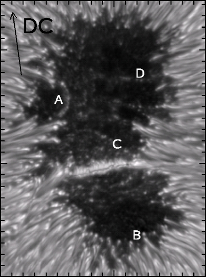
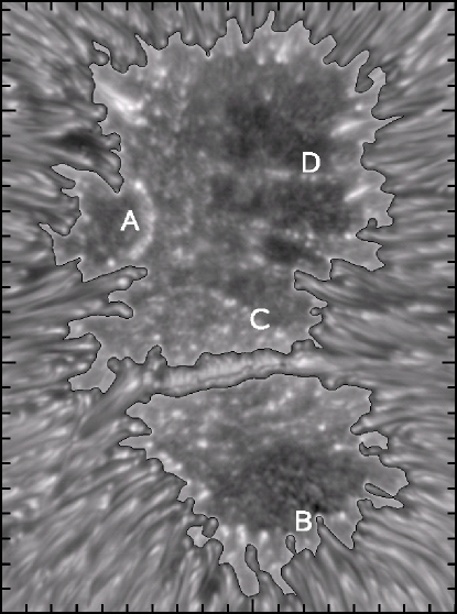
Abbildung 5.1: Frame taken at 09:53:20 UT: Best quality image plotted at normal contrast (left panel) and with increased umbral brightness (right panel). The black contour lines outline the umbra (see text for details). The direction to solar disk center (DC) is indicated by the arrow. Locations of umbral dots (UDs) that are discussed further in the text are marked by the letters A-D. Minor tick marks are given in Mm.

Our automated UD analysis starts with isolating the umbra, which is done by thresholding a lowpass filtered image (averaging a squared environment of 11 $\times$ 11 pixels) at 35 % of the mean intensity of the quiet photosphere ($I_{ph}$). From the resulting set of contours we select only those longer than 3 Mm in order to avoid larger UDs from being connected to the umbral boundary. In the particular case of the studied penumbra the results are almost identical to identifying the two longest contours with the umbral boundary. The thus obtained umbral boundary is visible in the right panel of Fig. 5.1 as the black contour line. This method for isolating the umbral boundary automatically ensures that a local brightening at the end of a penumbral fibril is only considered to be a UD if it is isolated from the penumbra in the sense that the intensity between the UD and the penumbral fibril falls below the applied threshold of 0.35 $I_{ph}$.

In the next step the UDs in each of the 310 images (recorded at a cadence of 20.57 s) are detected. For this purpose several algorithms were tested, e.g. a method where, starting from the UD center, 8 equally distributed rays are followed until they reach the UD boundary which is defined as the position where the intensity drops below 50 % of the maximum intensity above the local umbral background. The resulting 8 boundary points lead to a polygon that is a good approximation of the UD boundary. The method does not work properly for UDs with a partly concave boundary and it cannot easily separate UDs that are close to each other. Finally, the multilevel tracking algorithm of Bovelet & Wiehr (2001), which provided the best results in detecting the UD boundaries, was chosen. First the MLT algorithm determines the global extrema of the umbral intensities and subdivides this range into equidistant levels. Bovelet and Wiehr used MLT to distinguish between granules and intergranular lanes of the quiet Sun and found that three MLT levels are sufficient for their purpose. Since umbral dots cover a broad range of intensities we have to use a noticeably higher number of levels. We normalized our best quality image to $I_{ph}$ and found an umbral intensity range from 0.36-0.96 $I_{ph}$ (Note: This range is only valid for the best quality image, other images may reach lower or higher umbral intensities). We found that 25 MLT levels is the optimal compromise between detecting as many UDs as possible and avoiding the misinterpretation of noise as UDs. Whereas small umbral dots, obtained with this choice of levels, have a typical contrast relative to the local background of about 0.05 $I_{ph}$, the noise level is about 0.005 $I_{ph}$ (see Fig. 5.2 for a typical intensity profile). Starting with the highest intensity level all pixels are found whose intensity exceeds this level. This leads to several bounded two-dimensional structures, that are tagged in a unique way, which is indicated by different colors in the one-dimensional illustration given in Fig. 5.2. The obtained closed structures are extended pixel by pixel as long as the intensity is greater than the next lower level. After that the algorithm searches through the whole umbra again to find all pixels whose intensity is greater than the next lower level, which may lead to some newly detected closed structures. This procedure is repeated until the minimal intensity level is reached. At the end every umbral pixel belongs to exactly one closed structure. The mode of operation of the MLT algorithm is illustrated for one dimension in Fig. 5.2 for the case of 4 levels.

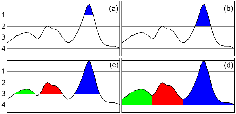
Abbildung 5.2: Illustration of multilevel tracking algorithm with 4 levels applied to a typical intensity profile.

The minimal ($I_{Min}$) and maximal ($I_{Peak}$) intensity of each closed structure is determined and all pixels that have an intensity lower than 50 % of this min-max range (white arrows in Fig. 5.3a) are cut. This leads to a first estimate of the UD boundaries (see Fig. 5.3b) that are used to determine the local umbral background intensities ($I_{bg}$), i.e. the intensities that would be observed in the absence of all UDs. We applied the method used by Sobotka & Hanslmeier (2005) that approximates the local umbral background by a 2D surface fitted to the grid of local intensity minima, using the method of thin-plate splines (Barrodale et al., 1993). Since the local umbral background intensities are known now (dashed line in Fig. 5.3c), we determine the exact UD boundaries by cutting all pixels lower than 50 % of the maximum intensity above the local umbral background (see white arrows in Fig. 5.3c). Fig. 5.3d illustrates that the resulting UD boundaries are similar to our first estimate in Fig. 5.3b so that we don’t need further iterations (this was the case with most identified UDs). Employing this procedure we found, on average, 323 UDs per image. Sometimes, our algorithm recognizes strong elongated bright structures as UDs that we would not consider as a UD by visual inspection of the images. Via a spot-check on selected images we estimate that the number of misidentifications is lower than 1 %. Due to the large number of detected UDs we are not able to remove the misidentifications by hand and accepted them as noise.

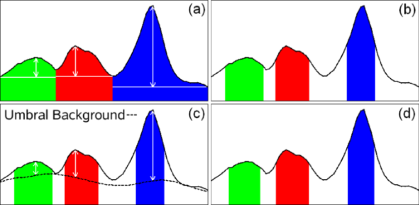
Abbildung 5.3: Determination of the boundary of umbral dots.

Since a UD is an extended structure we determine the coordinates of the brightest pixel (peak intensity) and save them as the UD’s position. This method is applicable because the noise was sufficiently reduced by our subsonic filter, as demonstrated by a typical intensity profile in Fig. 5.2. We also determine the UD’s diameter, defined as the diameter of a circle of area equal to that within the boundary of the UD. After the positions of all UDs of every image are known, the motions and trajectories of UDs are determined. The continuation of a trajectory in the image at the next (previous) time step is determined by finding the UD that is closest to the UD’s current position. If no UD can be found within a 5 pixel neighborhood (theoretical diffraction limit) of the current UD then the tracking stops. In a loop over all images every UD is tracked backward in time until its birth and forward in time until its death. The tracking must be tolerant to the occasional image with lower image quality in which the UD may not be correctly identified (specially the smaller and fainter ones). In practice we allow for a gap of up to two images. If a UD is present at nearly the same location on both sides of the gap, the tracking is continued. In this manner we found 12836 UD trajectories that are weakly lowpass filtered in space (averaging the positions of the same UD in 15 consecutive images) in order to further reduce seeing-induced noise. From now, we call such a smoothed trajectory simply $trajectory$. We note that 5949 of the 12836 UDs are only identified in a single image. We decided not to ignore them, because these bright dots in the umbra are detected rather well, even if only for a very short time. We assigned a zero trajectory length and a lifetime of 20.57 s to these 5949 UDs.

5.4 Results

5.4.1 Qualitative results

A first impression of the temporal evolution of the smallest umbral structures is reached by making a movie of the reconstructed time series of images. Some interesting phenomena are found by the visual inspection of this movie and are explained briefly below.

The sunspot has two umbrae, a smaller and a roughly twice larger one separated by a light bridge (LB). The LB contains a clearly visible dark lane in agreement with the observations of, e.g., Berger & Berdyugina (2003). The lane is closer to the limbward edge of the LB. Possibly this is because the sunspot was observed at a heliocentric angle of $\theta\leavevmode\nobreak\ =\leavevmode\nobreak\ \mathrm{18^{\circ}}$, so that projection effects may cause the observed asymmetry (e.g. Lites et al., 2004). However, the LB also displays another major asymmetry: the movie exhibits many UDs that are born within the LB and move into the larger umbra, i.e. towards the solar disk center (arrow in Fig. 5.1), while almost no UD leaves the LB into the smaller umbra, i.e. towards the solar limb (antiparallel to the arrow).

The data clearly show that bright UDs often form chains. The most prominent chains often start from a penumbral filament and UDs are found to move along the chain until they dissolve. The horizontal motion of the UDs is preferentially along the chain and is directed from the ends of the chain to its center, where the UDs disappear. Fig. 5.4 displays the most prominent chain of UDs in the observed umbra. The length of this chain is about 3200 km and it is about 350 km wide. In the left panel, from 08:58:56 UT, the chain appears as a simple succession of UDs. One can see the same region in the right panel 28 minutes later. The appearance of the chain changed and now the lower part of the chain looks similar to a narrow light bridge. The typical dark lane of a LB can be seen clearly, even if we degrade the image quality to the lower level of the left panel by convoluting the image with a point spread function of a circular pupil (not shown). This degradation was carried out to compensate for the higher spatial resolution of the later image. High spatial resolution is demonstrated by the presence of dark-cored penumbral filaments (see Langhans et al., 2007), which are generally observed only at the highest resolution in the blue. The presence of the dark lane is an indication that the chain eventually evolved into a fully developed LB some hours after the end of the recording (Katsukawa et al., 2007).

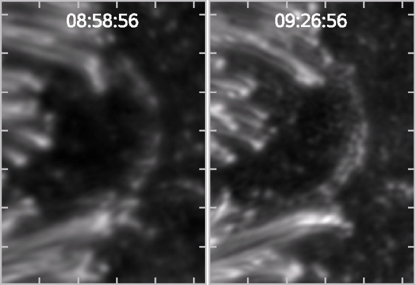
Abbildung 5.4: Most prominent chain of umbral dots in the studied umbra, located near label A in Fig. 5.1 (FOV is 5.4 $\times$ 7.4 Mm). The left panel shows the chain composed of several typical UDs along a curved line at 08:58:56 UT. The right panel shows the same chain 28 min later. At this later time the lower half of the chain looks similar to a narrow light bridge. The typical dark lane is clearly recognizable.

In some exceptional cases we observe the splitting of a single UD into two parts that continue their life as independent UDs. Such a splitting is displayed in Fig. 5.5. It concerns a UD located close to the penumbra, near point B in Fig. 5.1. The opposite case, the merging of two UDs into a single one, can also be observed in a few rare cases: See Fig. 5.6 for an example. Nearly identical phenomena in the temporal evolution of penumbral grains were observed by Hirzberger et al. (2002).

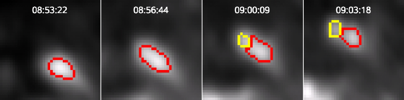
Abbildung 5.5: Splitting of an umbral dot near the position B in Fig. 5.1 (FOV is 1.2 $\times$ 1.2 Mm). The red and yellow lines are the UD boundaries as detected by the method explained in the main text.

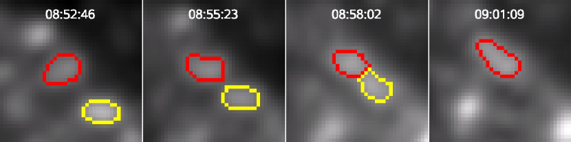
Abbildung 5.6: Merging of two umbral dots near position C in Fig. 5.1 (FOV is 1.2 $\times$ 1.2 Mm).

An interesting sequence of events is illustrated in Fig. 5.7. First the merging of two UDs can be observed followed immediately afterwards by the splitting of the resulting, unified UD into two new UDs. The sequence looks similar to an elastic impact in a Newton pendulum consisting of two balls: The nearly motionless UD 1 is hit by the moving UD 2. The impact of the two UDs brings the second UD to a standstill while the first UD starts to move roughly in the direction of the first UD. Note that this is simply an empirical description and we do not propose that this is what physically happens (or that the unified UD breaks up into the same parcels of gas which united to form it).

If two UDs come close to each other then the visual impression of a single UD exhibiting a dark lane can occur, see last panel of Fig. 5.7 for an example. None of the UDs in our data set seems to stay in such a state for a significant fraction of the UD lifetime. Since the dark lanes as seen in the simulations of Schüssler & Vögler (2006) are visible for most of the UD lifetime, we conclude that we find no clear evidence for such dark lanes. This difference to the results of Bharti et al. (2007) and Rimmele (2008) may stem from the different wavelengths of the analyzed data. The wavelength can have a remarkable effect on the detected fine structure (e.g. Zakharov et al., 2008).

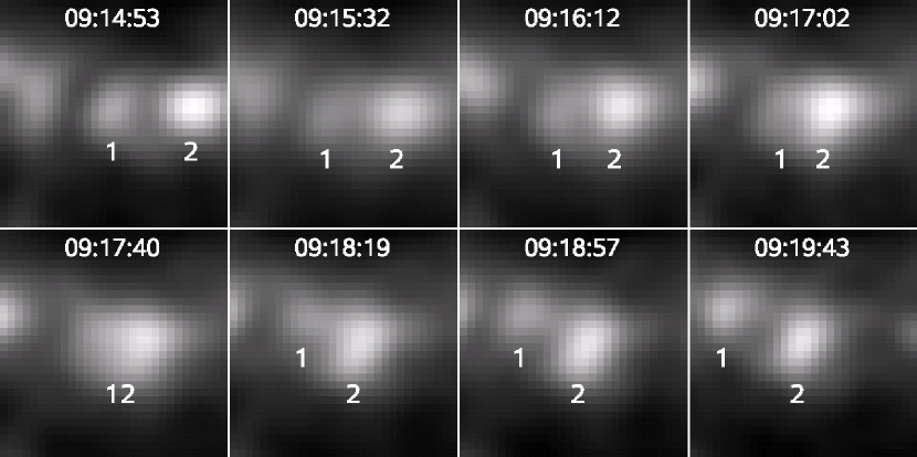
Abbildung 5.7: Elastic collision of two umbral dots. The sequence of events is seen near the position marked D in Fig. 5.1 (FOV is 0.9 $\times$ 0.9 Mm). UD 2 moves towards UD 1 and merges with it, before separating from it again.

The properties of a UD change along its trajectory. In order to assign a property to the entire trajectory we either average over all points along the trajectory (which is expressed by introducing an upper index Mean") or we determine the maximum value reached by that parameter over all trajectory points (which is expressed by the upper index Max"), e.g., $D^{Mean}$ means the UD diameter averaged along the trajectory, while $I_{Peak}^{Max}$ is the maximum value of all peak intensities along a UD trajectory (where the peak intensity is the largest intensity within the UD boundary at a given point in time).

Fig. 5.8 shows the best image with all identified UDs marked by circles. The circles are centered on the positions of $I_{Peak}^{Max}$, i.e. the position of maximum intensity. In the left panel the circles have a constant radius, while their radii are proportional to $I_{Peak}^{Max}$ in the right panel. As a result we get an impression of the spatial distribution of UD occurrence as well as of the spatial distribution of UD brightness. Obviously, there is hardly any part of the umbra which does not support umbral dots. Only very localized small voids are visible. The brightness distribution of UDs, however, is rather inhomogeneous, with clear concentrations of bright UDs and regions harboring mainly dark UDs (mainly in the upper right part of the upper umbra and in the lower part of the lower one). Since the UDs of a chain (like the chain close to label A in Fig. 5.1 and shown in more detail in Fig. 5.4) appear to move along the chain and hardly in the direction perpendicular to it, there is often a narrow void directly beside the chain.

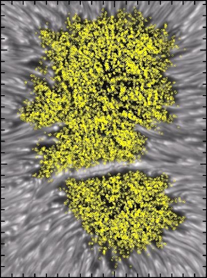
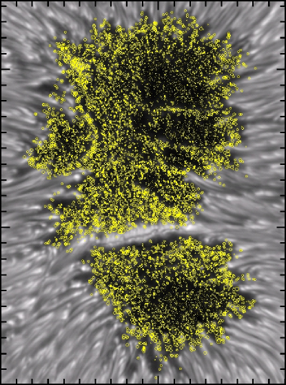
Abbildung 5.8: Spatial distribution of UD occurrence (left panel) and UD maximum brightness (right panel). Each UD is plotted only once along its entire trajectory, at the position of its maximum brightness.

5.4.2 Quantitative properties

The filling factor, i.e. the sum of all UD areas relative to the total umbral area, is correlated to the image quality. Essentially, the filling factor is constant over the entire period of observations (see Fig. 5.9), which is important for the later determination of the time dependence of their properties. On average we determine a value of about 11 %. Fig. 5.9 shows also the image contrast from an undisturbed granulation area outside the sunspot which demonstrates the high homogeneity of the image quality in our time series.

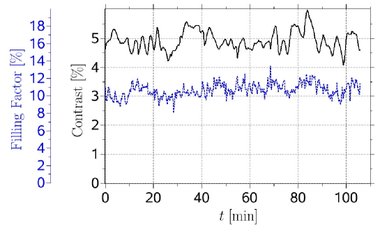
Abbildung 5.9: Dependence of UD filling factor (dotted blue line) and granulation contrast (solid black line) on the interval of time, $t$, since the first image of the series was recorded.

The histogram of the UD lifetimes is displayed in Fig. 5.10 with a logarithmic $y$ axis. One can see that most of the UDs live for a short time. These short-lived UDs move over short distances which leads to physically nonsensical velocities due to the discretization of lifetime and distance. Consequently, when discussing trajectories and velocities of UDs we only consider the 2899 trajectories of UDs with lifetimes greater than 150 s. The histogram is nearly linear for lifetimes between 5 and 60 minutes, which, due to the logarithmic vertical scale, suggests an exponential distribution of lifetimes. The excess of UDs with short lifetimes may partly be due to seeing. Also given in Fig. 5.10 is the mean lifetime (180 s) and the median lifetime (41 s). If we consider only the 2899 trajectories of UDs with lifetimes greater than 150 s then we find a mean lifetime of 630 s and a median of 390 s. Note that 281 UDs are already present in the first image and 344 UDs are still present in the last image, whereas only one UD survives the whole sequence. Ignoring those 625 UDs reduces the mean lifetime from 180 s to 152 s. The median lifetime as well as the shape of the histogram do not change, because the number of incomplete UD trajectories is small compared to the total number of UDs. Thus we decided to neglect this effect and consider all 12836 UDs in the following text.

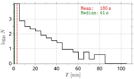
Abbildung 5.10: Histogram of lifetimes $T$ of all 12836 UD trajectories (solid line) and their mean and median value (dashed lines and text labels). The bin size is 300 s.

The histogram of the mean UD diameters is plotted in Fig. 5.11 a. The mean UD diameters vary between 50 and 750 km. The UDs have a mean diameter of around 229 km and 95 % of the UDs are spatially resolved at our diffraction limit of 130 km. Sobotka & Hanslmeier (2005) found 175 km for the mean UD diameter. They determined the UD boundaries by finding all pixels with downward concavity, whereas we used all pixels whose intensity is greater than 50 % of the $I_{Peak}-I_{bg}$ range, $\Delta I_{thresh}=(I_{thresh}-I_{bg})/(I_{Peak}-I_{bg})=0.5$. As one can see in Fig. 5.12 we would also find a mean UD diameter of 175 km if a threshold of about $\Delta I_{thresh}=0.67$ would be used. Nevertheless, we prefer to continue our analysis with a value of 0.5 in analogy to the FWHM definition. Clearly, the employed threshold influences the filling factor as well, roughly quadratically. Remarkably, the histogram is nearly symmetric, which supports the conclusion that most UDs have been resolved.

The histogram of the mean horizontal velocities, i.e. the quotient of trajectory length and lifetime, is plotted in Fig. 5.11 b and exhibits a broad distribution from 0 to more than 1 km s^-1 with a significant maximum at 350 m s^-1. The velocity distribution is slightly asymmetric with a small tail to higher velocities. Fig. 5.11 c shows the histogram of the mean peak intensities, i.e. the mean of all peak intensities of the points along the trajectory. All intensities are normalized to the mean intensity of the quiet photosphere ($I_{ph}$). Just 3 of the 12836 UDs reach a brightness greater than that of the quiet Sun, whereas most of the UDs are about half as bright as the quiet photosphere. The distribution is asymmetric, with a tail to higher intensities. Note that these brightnesses are strongly wavelength dependent and cannot be easily compared with values published in the literature (Solanki, 2003). Lastly, the histogram of the distances between the UD’s birth and death position ($L_{BD}$) is given in Fig. 5.11 d. With increasing distance the number of UDs decreases exponentially, so that only a few UDs travel over long distances in their life, most UDs do not leave the vicinity of their birth position. The maximum observed birth-death distance is 2 Mm, about 20 % of the upper umbra’s diameter of roughly 10 Mm.

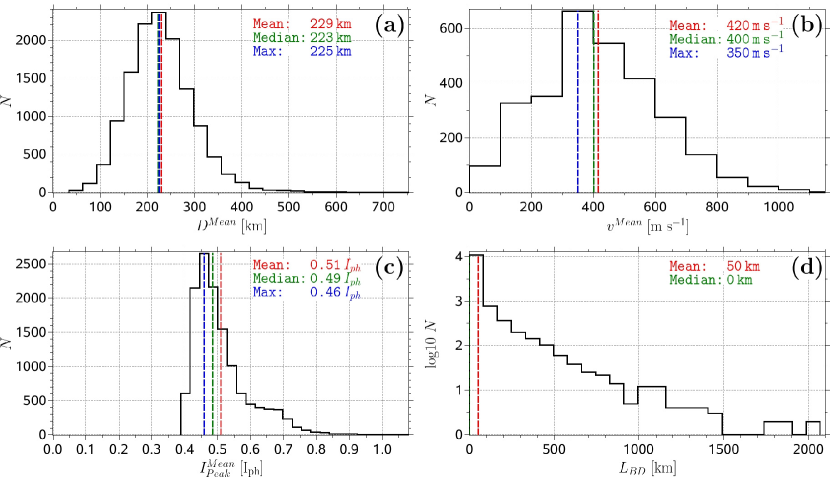
Abbildung 5.11: Histogram of mean diameters (a), mean horizontal velocities (b), mean peak intensities (c), and distances between birth and death position (d). (a), (c), and (d) are plotted for all 12836 UD trajectories and (b) for the 2899 trajectories of UDs that lived longer than 150 s. The location of the maximum, the mean, and the median of the distribution is indicated in each frame. The bin sizes are 30 km for (a), 100 m s^-1 for (b), 0.03 $I_{ph}$ for (c), and 90 km for (d).

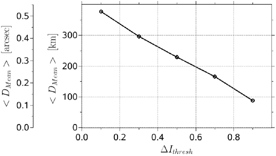
Abbildung 5.12: Mean UD diameter averaged over all trajectories as a function of the intensity threshold $\Delta I_{thresh}$ (defined in main text) that is used to determine the UD boundaries (see also Fig. 5.3 and its explanation).

A UD size versus UD peak intensity scatterplot (Fig. 5.13) reveals that there is a weak correlation between UD size and brightness. The brightest UDs are not the biggest ones and large UDs are not the brightest ones. The solid green line connects binned values (obtained by averaging 100 data points with similar intensities) and shows that bright UDs are on average a bit larger than small ones. The relation found by Tritschler & Schmidt (2002) is qualitatively confirmed, although they only considered UD intensities in individual snapshots while we tracked the temporal development of the UDs over their lifetimes.

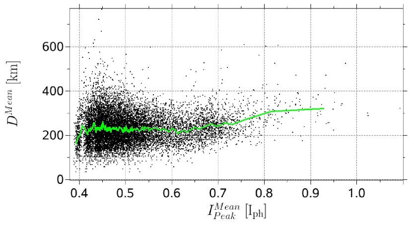
Abbildung 5.13: Scatterplot of mean UD diameter versus mean peak intensity. The solid green line connects binned values.

The relation between a UD’s mean size (i.e. the size averaged over the lifetime) and its lifetime is plotted in Fig. 5.14 (the green curve is obtained after binning over 100 data points). The binned values show an increase in $D^{Mean}$ with increasing lifetimes for short-lived UDs. For the longer lived ones size and lifetime do not correlate. The UD sizes scatter more for short lifetimes. All long-lived UDs are of intermediate size of around 290 km. The large, short-lived UDs are all present in the first image of the time series, so that their lifetime would actually be larger if we had started our observation earlier.

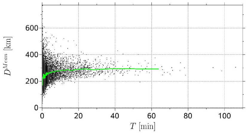
Abbildung 5.14: Scatterplot of mean UD size versus lifetime. The solid green line connects binned values.

In the literature we often find a separation into two UD classes, e.g. Grossmann-Doerth et al. (1986) find a difference between peripheral and central UDs, i.e. between UDs that are born close to the umbra-penumbra boundary and UDs that are born deep in the umbra, whereas Hartkorn & Rimmele (2003) and Sobotka et al. (1997b) distinguish bright and dark UDs. We use different properties to find reasonable distinctions between types of UDs. E.g. from now on a given UD is called a peripheral UD (PUD) if the UD’s birth position is closer than 400 km to the umbral boundary, otherwise it is termed a central UD (CUD). (The selected threshold comes from the histogram of the distances between the UD’s birth position and the umbral boundary (not shown) which shows a maximum at around 400 km.) Alternatively, if the distance traveled between birth and death position is larger than 750 km then we call it a mobile UD, otherwise a stationary UD. (We plotted the trajectories of all UDs whose $L_{BD}$ was greater than a threshold, which was determined by starting at a small value and increasing it step by step. We stopped at 750 km which is the smallest $L_{BD}$ at which no trajectories occurred anymore in the central part of the umbra.) The aim here is not to separate UDs into distinct classes by a single property, e.g. a histogram of $L_{BD}$ (Fig. 5.11 d) does not show two peaks, even if restricted to long-lived UDs. However, as we shall see below the most mobile UDs are formed near the penumbra, while the least mobile ones are mainly formed deep in the umbra. Such a distinction may help to guide theory towards a better understanding of the origin and evolution of UDs with different properties and at different locations.

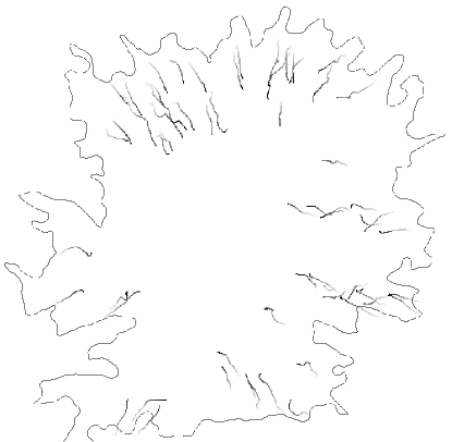
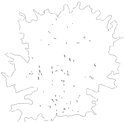
Abbildung 5.15: UD trajectories in the upper umbra. The bright ends of the trajectories denote the positions of the UD’s birth and the dark ends show the position at death. The black contour line corresponds to the umbral boundary as detected in the best quality image. The left panel shows all UDs whose distance between the birth and the death position was greater than 750 km, the right panel shows all UDs with a birth-death distance smaller than 150 km whose lifetime was greater than 800 s.

The strong concentration of bright UDs near the umbral boundary (or along proto-light bridges) is already clear from Fig. 5.8 (right panel). Fig. 5.15 shows a separation by birth-death distance. The left panel displays the longest UD trajectories, i.e. only the mobile UDs are shown. These UDs are also relatively long-lived. (Smallest lifetime of this UD class, that contains 85 UDs, is 15 min.) The right panel shows trajectories of long-lived UDs with a small birth-death distance. A clear separation by the birth position is readily identifiable. Almost all trajectories with a large birth-death distance start close to the umbra-penumbra boundary and these UDs move nearly radially into the umbra. A visual inspection of the movie of the reconstructed time series of images shows that many of these UDs are former penumbral grains that broke away from the penumbra. In contrast, many of the UDs with a small birth-death distance are born in the umbral interior and move along a closed loop or jitter around their birth position. We cannot say if this jitter has a physical background or if it is caused by residual seeing-induced noise. As mentioned in section 5.3 we determined the umbral boundary individually for each image but we show only that corresponding to the best quality image as black contour line in Fig. 5.15, 5.17, and 5.18. Consequently some trajectories (or parts of them) are outside the black contour line, although they are always inside the umbra at the time of their occurrence (see, e.g., the bottom-left corner of the left plot of Fig. 5.15).

Let us now consider more quantitatively the fact that the mobile UDs prefer to move radially towards the umbral center. Fig. 5.16 displays a histogram of the UD’s deflection angles $\alpha_{\rm{defl}}$ that is defined as angle between the line connecting the umbral center and the UD’s birth position and the line connecting the UD’s birth and death position. Radially directed inward flow will lead to $\alpha_{\rm{defl}}\leavevmode\nobreak\ =\leavevmode\nobreak\ \mathrm{0^{\circ}}$ and an outward flow to $\alpha_{\rm{defl}}\leavevmode\nobreak\ =\leavevmode\nobreak\ \mathrm{180^{\circ}}$. Obviously, this definition makes sense only for the 5689 UD trajectories that have different birth and death positions. The solid black line in Fig. 5.16 shows the histogram for all these UDs and exhibits a clear tendency for a radially directed inward motion (42 % of the UDs are found to have a deflection angle lower than $\mathrm{45^{\circ}}$). This tendency is much more significant if we only consider mobile UDs, see the dotted blue line (88 % of the mobile UDs are found to have a deflection angle lower than $\mathrm{45^{\circ}}$). However, histograms calculated for central UDs and for peripheral UDs (not shown) lead, in principle, to the same shape as for all UDs, i.e. UDs born close to the penumbra do not show a significantly higher tendency of radially inward directed motion than the central UDs.

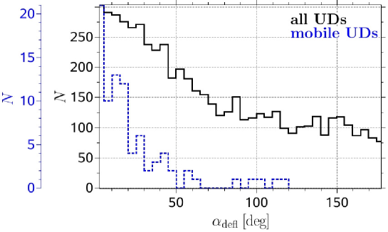
Abbildung 5.16: Histogram of radial deflection angles $\alpha_{\rm{defl}}$ of all UD trajectories (solid black line) and of the mobile UD trajectories (dotted blue line).

The trajectories of large UDs are drawn in Fig. 5.17 (left panel). They are born throughout the umbra, with a tendency to cluster in the darker part of the umbra. The vicinity of the light bridge is avoided. This UD class contains long trajectories as well as short ones. The trajectories of the brightest UDs can be seen in the right panel of Fig. 5.17. These UDs all emerge close to the penumbra, the light bridge, or the prominent UD chain (label A in Fig. 5.1).

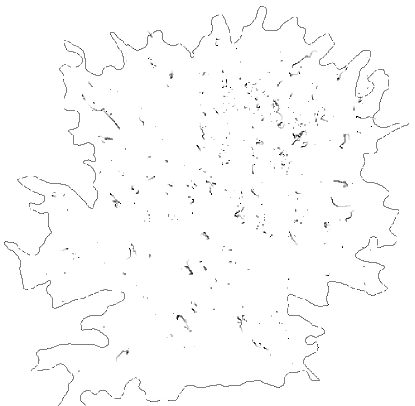
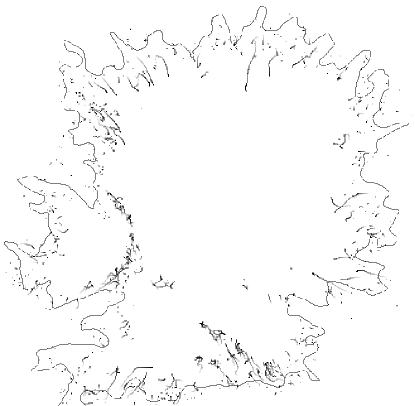
Abbildung 5.17: UD trajectories in the upper umbra. The left panel shows all UDs with mean diameter greater than 350 km and the right panel shows all UDs with a mean peak intensity greater than 0.65 $I_{ph}$.

Many UDs with a preferred direction of motion arise near the light bridge. Most of the UDs that emerge on the disk center side of the light bridge (i.e. into the large umbra) move away from the light bridge while many of the limbside UDs (i.e. those formed in the small umbra) move towards the light bridge (see Fig. 5.18). A high density of UDs is formed by splitting off the light bridge, but all in one direction, in which the LB is corrugated and unsharp (disk center, large umbra side), while on its other straight and sharp side nearly no UDs leave the LB.

Abbildung 5.18: UD trajectories near the light bridge with birth-death distance greater than 300 km.

Tabelle 5.1: Characteristic values of UD parameters for different UD classes defined in the main text.

Class	Condition	$N$	$D^{Mean}$	$v^{Mean}$	$I_{Peak}^{Mean}$	$(I_{Peak}/I_{bg})^{Mean}$	$T$	$L_{BD}$	$L_{Traj}$
			[km]	[m s-1]	[$I_{ph}$]		[s]	[km]	[km]
all UDs		12836	229$\pm$68		O.51$\pm$O.O9	1.1O$\pm$O.O8	18O$\pm$39O	5O$\pm$13O	7O$\pm$2OO
all UDs	$T>$15O s	2899	272$\pm$53	42O$\pm$19O	O.55$\pm$O.1O	1.17$\pm$O.1O	63O$\pm$63O	19O$\pm$22O	29O$\pm$35O
peripheral UDs	$T>$15O s	621	252$\pm$44	45O$\pm$21O	O.65$\pm$O.O7	1.23$\pm$O.11	56O$\pm$55O	21O$\pm$25O	29O$\pm$35O
central UDs	$T>$15O s	2278	278$\pm$53	41O$\pm$19O	O.53$\pm$O.O9	1.15$\pm$O.O9	65O$\pm$65O	18O$\pm$21O	3OO$\pm$35O
mobile UDs	$T>$15O s	85	287$\pm$33	68O$\pm$14O	O.64$\pm$O.O8	1.29$\pm$O.O9	227O$\pm$83O	1O8O$\pm$3OO	147O$\pm$41O
stationary UDs	$T>$15O s	2814	272$\pm$53	41O$\pm$19O	O.55$\pm$O.1O	1.16$\pm$O.1O	58O$\pm$55O	16O$\pm$15O	26O$\pm$27O
chain A UDs	$T>$15O s	48	3O1$\pm$45	48O$\pm$19O	O.68$\pm$O.O6	1.29$\pm$O.O8	96O$\pm$71O	24O$\pm$23O	48O$\pm$4OO
light bridge UDs	$T>$15O s	217	254$\pm$41	43O$\pm$19O	O.64$\pm$O.O8	1.23$\pm$O.11	8OO$\pm$8OO	22O$\pm$24O	37O$\pm$43O

The mean diameter $D^{Mean}$, mean horizontal velocity $v^{Mean}$, mean peak intensity $I_{Peak}^{Mean}$, mean intensity contrast $(I_{Peak}/I_{bg})^{Mean}$, lifetime $T$, birth-death distance $L_{BD}$, trajectory length $L_{Traj}$ (see definitions of these quantities in the previous text), and the number of UDs $N$ of the types or classes mentioned earlier in this section are summarized in Table 5.1. We averaged over all trajectories of a UD class. The standard deviation $\sigma$ is given after each average value. As mentioned earlier, we consider only UDs that lived longer than 150 s in all cases in which we calculate the mean velocity; only the first line includes all UDs. The last two rows consider only UDs that are close to chain A or the light bridge, respectively. According to Table 5.1 the difference between peripheral UDs and central UDs is not so large (using the simple categorization described above). The largest relative difference is in the brightness. For all other parameters the difference is less than $1\sigma$. In contrast to that, the difference between mobile UDs and stationary UDs is more significant. A relatively large difference of more than $1\sigma$ is found for the mean horizontal velocity, for the mean intensity contrast, for the lifetime, and, again for the brightness. On average mobile UDs are brighter, they move faster, and they live longer than stationary UDs but they have similar sizes.

Sometimes one can observe complete chains of successive UDs that are very close to each other (see label A in Fig. 5.1 and the left panel of Fig. 5.4). According to Table 5.1 these UDs are relatively bright and they move along the chain from the endpoints of the chain towards its center, where they disappear. Their mean peak intensity is 0.68 $I_{ph}$ which is significantly higher than 0.51 $I_{ph}$, the average of all UDs, but is comparable to that of the peripheral and mobile UDs. The mean diameter as well as the mean velocity of the UDs within the chain is slightly above average. Table 5.1 also reveals that UDs that are born close to the light bridge show on average a significantly higher brightness and contrast than the mean UD but all other properties do not show remarkable differences.

The umbral background is brightest near the penumbra and gets darker towards the center of the umbra. Fig. 5.19 shows that the UD peak intensity correlates with the umbral background intensity, with the mean ratio $I_{Peak}/I_{bg}$ = 1.2 $\pm$ 0.1 (intensity contrast). Sobotka & Hanslmeier (2005) found an intensity contrast of 1.8 for a wavelength of 451 nm and 1.6 for the wavelength 602 nm. Obviously, the intensity contrast not only depends on the wavelengths but also on the spatial resolution that can be slightly different even if we compare data from the same telescope. Additionally, the intensity contrast can also be affected by the subsonic filter and the MFBD image restoration we applied. Importantly, however, both binning the points in Fig. 5.19 (solid green curve) and a linear regression (dotted red curve) indicate that the contrast increases nearly linearly with $I_{bg}$. A scatter plot of the UD intensity contrast versus the shortest distance between the UD birth position and the penumbra (not shown) reveals that this UD contrast is not constant over the umbra. The closer the UD is born to the penumbra the higher its intensity contrast, although the contrast does not drop as rapidly from the umbral boundary as the UD brightness does, so that partly, the dependence on distance is due to the dependence on $I_{bg}$ (Fig. 5.19). We also found that on average the long-lived UDs have a higher contrast than the short-lived ones.

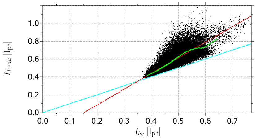
Abbildung 5.19: UD peak intensity versus umbral background intensity. The solid green line connects binned values. The dashed cyan line displays the theoretical, lower limit of the peak intensities. A linear fit to the data results in the dotted red line.

In a further step we subdivided the umbra into several boxes and determined the probability that a UD is born in such a box. The map obtained in this manner shows a uniform distribution of the UD birth probability (not plotted). Only for very small box sizes do the dark umbral nuclei (see left panel of Fig. 5.8) become visible as locations of reduced UD production.

Finally, we are interested in the temporal evolution of the UD properties over their lifetimes. To this end we normalize all UD lifetimes to unity and average the temporal evolution of the diameters, peak intensities, intensity contrasts ($I_{Peak}/I_{bg}$), and horizontal velocities of the 2899 trajectories with $T\leavevmode\nobreak\ >\leavevmode\nobreak\ 150\leavevmode\nobreak\ s$. In order to weight all trajectories equally, i.e. independently of their lifetime, we up-sample all trajectories to 310 points of time via interpolation. (Our time series contains 310 images, so that no trajectory can consist of more than 310 points.) Then we averaged the UD parameters with the help of our binning method, which is applied separately for the 621 PUDs and the 2278 CUDs. Each bin contains 15000 points for PUDs and 50000 points for CUDs. The results are plotted in Fig. 5.20 and show that the mean PUD is smaller, brighter and moves faster than the mean CUD (as could already be deduced from Table 5.1). More importantly, there are distinct differences in their mean evolution. Whereas both types of UDs share the property that their diameters evolve rather moderately over time (the increase after birth and the decrease before death are less than 10 % of the maximum diameter (see panel a), the evolution of their brightness (panel b) and in particular of their contrast (panel c) differ considerably. While the mean CUD displays an initial gentle brightening followed by an equally gentle darkening, the mean PUD darkens continuously. The small magnitude of the change in brightness may be due to the fact that we have averaged over UDs with very different absolute intensity. More information may be gleaned from the contrast, i.e. the peak intensity divided by the local umbral background intensity, plotted in panel (c). The mean PUD initially remains almost constant, exhibiting a slight maximum at around 1/3 of the mean lifetime before dropping rapidly over the remaining portion of its life. The contrast of the CUDs displays a much more symmetric evolution. The birth velocity of the mean PUD is nearly 50 m s^-1 higher than for the mean CUD, while the velocity at death of the two UD types is similar, see panel (d). Both velocity curves show an initial increase, followed by a decrease. As in the case of the contrast the velocity profile is much more symmetric for the CUDs.

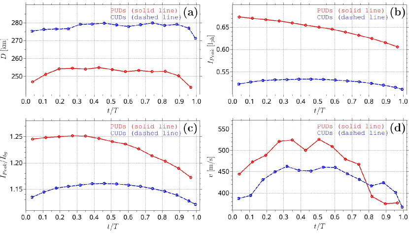
Abbildung 5.20: Temporal evolution of the UD diameter (a), UD peak intensity (b), intensity contrast (c), and velocity (d) separated for peripheral UDs (solid red line) and central UDs (dashed blue line). The UD lifetime is normalized to unity.

5.5 Discussion and conclusions

We have analyzed a time series of images of a mature sunspot close to solar disk center. Due to the excellent image quality we were able to resolve thousands of UDs. Exhaustive UD analyses can be found in earlier papers (Sobotka et al., 1997a, b; Hartkorn & Rimmele, 2003; Sobotka & Hanslmeier, 2005; Sobotka, 2006), but the present article is the first detailed UD study of a long time series of reconstructed images with the consistent high resolution of a 1-meter telescope.

Trajectories, lifetimes, diameters, horizontal velocities, peak intensities, and distances between birth and death locations were determined by tracking single UDs over the time series. These characteristic values were used to look for reasonable separations into UD classes. In the following we summarize the obtained results and compare them with other investigations in the literature:

1. There is hardly any part of the umbra which does not support UDs, but the UD brightnesses depend strongly on the location within the umbra, which confirms the previous observation of Sobotka et al. (1997b).

2. The histogram of lifetimes shows an exponential distribution, i.e. a UD does not have a typical lifetime. More than 3/4 of all studied UDs lived less than 150 s and their motion was negligible. The exponential distribution is in qualitative agreement with the results obtained by Sobotka et al. (1997a, 1999). Quantitatively, Sobotka et al. (1997a) obtains a median lifetime of 6 min for an umbra of about 6 Mm diameter and a median of 12 min for a 4 Mm pore (Sobotka et al., 1999), whereas we find a median value of 0.7 min for a roughly 10 Mm umbra. Note that these median values depend strongly on algorithmic constraints as well as on the cadence of the time series. For example, the method used by Sobotka et al. (1997a) cannot lead to lifetimes shorter than 1.5 min. If we only consider UDs with lifetimes greater than 1.5 min our median increases to 4.1 min. Irrespectively of which of these two values we use, our results are consistent with the conclusion of Sobotka et al. (1999) that UDs are more stable in a weak magnetic field if we assume a direct correlation between umbral diameter and magnetic field strength (cf. Kopp & Rabin, 1992). Alternatively, due to the strong dependence of umbral brightness on umbral size (Mathew et al., 2007) the lifetime may be influenced mainly by the radiative flux or umbral temperature. The scatterplot of the mean umbral background intensities versus the UD lifetimes (not shown) is consistent with both possible explanations mentioned above: UDs live longer in brighter parts of the umbra. Due to the non-linear, monotonically decreasing relation between magnetic field strength and background intensity as observed by Kopp & Rabin (1992) and confirmed by Martínez & Vázquez (1993); Solanki et al. (1993), this implies that UDs live longer in regions of weak field.

3. The histogram of mean diameters exhibits a maximum at 225 km (0.31^′′) and descends from there towards the diffraction limit, so that we expect the majority of UDs to have been spatially resolved. This seems not to be the case in many of the earlier papers because there a monotonic decrease was obtained towards higher diameters (see Sobotka et al., 1997a, 1999). Sobotka & Hanslmeier (2005) also analyzed data obtained with the 1-meter SST. These data lead to a histogram that is qualitatively similar to ours. The mean diameter of 175 km (0.24^′′), as well as the average filling factor of 9 % is, however, noticeable smaller. This difference can be explained by the use of a different method to determine the UD boundary. An increase of our brightness threshold to determine the UD boundary leads to smaller diameters and to lower filling factors. Hamedivafa (2008) used an improved method of image segmentation and also found a mean diameter of 230 km and a similar shaped histogram.

4. The mean horizontal velocity of those of our UDs that live longer than 150 s is 420 m s^-1 which is significantly higher than the 210 m s^-1 reported by Molowny-Horas (1994) and higher than the 320 m s^-1 found by Sobotka et al. (1999). In both studies the mean horizontal velocity was calculated by means of least-squares linear fits of the x and y coordinates of all trajectory points, which leads to an underestimation of velocity in case of curved trajectories. Our histogram of horizontal velocities shows a maximum at 350 m s^-1, whereas some UDs can reach velocities above 1 km s^-1. This is in qualitative agreement with the histograms of Kitai (1986), Molowny-Horas (1994), and Hamedivafa (2008) but disagrees with the results of Sobotka et al. (1997b, 1999) whose histograms do not exhibit a maximum; they peak at zero velocity and show a monotonic decrease toward higher velocities of up to 1 km s^-1. The majority of our UDs moves irregularly around the birth position. However, there are some mobile UDs that travel over long distances within their lifetime. Almost all mobile UDs emerge close to the umbral border, i.e. near the penumbra, they are brighter than the average and their horizontal motion is preferentially directed towards the center of the umbra. The mean velocity of our mobile UDs is 680 m s^-1, which is in good agreement with the recent observation of Katsukawa et al. (2007) who found a mean velocity of 700 m s^-1.

5. The relation between mean UD size and lifetime is non-linear. On average, the size of UDs increases with lifetime, which was also found by Sobotka et al. (1997a), but in contrast to their work we find a narrow size distribution of around 290 km for long-lived UDs.

6. UDs that were born close to the penumbra show a significantly higher contrast than the UDs of the umbral interior. The mean UD intensity contrast $I_{Peak}/I_{bg}$ is 1.2 which is smaller than the value of 1.6 reported by Sobotka & Hanslmeier (2005). This may partly be due to the longer wavelength of our observation. Additionally, our statistical ensemble contains many more UDs. In particular we took many UDs with low contrast into account, made possible by the multilevel tracking technique (Bovelet & Wiehr, 2001) we employed to identify UDs. Consequently, we believe that the lower UD contrast we find is not due to a lower resolution or higher stray light, but rather to differences in identification of UDs and in particular the difference in wavelength. We stress that the UD contrast itself depends on the background intensity; the higher the intensity the stronger the contrast. Also it cannot be ruled out that there could be systematically different contrasts between different sunspots due to intrinsicly different physical properties of the spots.

7. Whereas the temporal variation of the UD diameter is qualitatively similar for UDs formed close to the penumbra (PUDs) and those formed in the body of the umbra (CUDs), their intensity contrast and horizontal velocity display contrasting evolutions. The mean PUD shows a continuous darkening which is in agreement with the results of Kitai et al. (2007) for a single typical PUD. The typical CUD of Kitai et al. (2007) is found to increase in brightness linearly and then to darken linearly with time, whereas our results for the mean CUD show a non-linear increase in brightness until nearby half of the lifetime followed by an again non-linear decrease. The clear difference between PUDs and CUDs in the behavior of their contrast and mean velocity may be a result of the different origin of the two types of features (Kitai et al., 2007). We confirm from visual inspection of a subset of PUDs that PUDs are formed when penumbral grains cross the umbral boundary.

A comparison of the results with the simulations of Schüssler & Vögler (2006) shows a better agreement with CUDs, than PUDs. For example, the simulated UDs display a gradual increase in contrast followed by a gradual decrease, just as CUDs. They also display little proper motion. This qualitative agreement further strengthens the interpretation of UDs as localized columns of overturning convection proposed by Schüssler & Vögler (2006). Hinode data had earlier suggested the presence of dark lanes in large UDs (Bharti et al., 2007) and revealed a decrease in the magnetic field strength with depth, as well as an upflow associated with a temperature enhancement (Riethmüller et al., 2008c), in good qualitative agreement with the simulations. A detailed analysis of the simulations similar to the one carried out here would allow a more quantitative comparison.

The PUDs have significantly different evolution histories than the simulated features. They start at a higher speed (Kitai, 1986) and in particular display their maximum brightness right after the beginning of their life (cf. Kitai et al., 2007). This, combined with the fact that they are born very close to the penumbra, or actually by breaking away from the penumbra (Thomas & Weiss, 2004), and move radially towards the umbral center (Kitai, 1986) supports that these are two distinct types of UDs based on their origin and evolution, although their physical structure is relatively similar (Riethmüller et al., 2008c).

Kapitel 6 Stratifications of sunspot umbral dots from inversion of Stokes profiles recorded by Hinode¹

6.1 Introduction

The energy transport immediately below the solar surface is mainly determined by convective processes that are visible as granulation patterns in white-light images of the quiet photosphere. This convection is suppressed inside sunspot umbrae due to the strong vertical magnetic field, but some form of magnetoconvection (Weiss, 2002) is needed to explain the observed umbral brightnesses. Umbral fine structure such as light bridges or umbral dots (UDs), dotlike bright features inside umbrae, may well be manifestations of magnetoconvection. Different models have been proposed to explain UDs, e.g., columns of field-free hot gas in between a bundle of thin magnetic flux ropes (Parker, 1979; Choudhuri, 1986), or spatially modulated oscillations in a strong magnetic field (Weiss et al., 1990). Recent numerical simulations of three-dimensional radiative magnetoconvection (Schüssler & Vögler, 2006) reveal convective plumes that penetrate through the solar surface and look very much like UDs. Although recent broadband images may have spatially resolved UDs (Sobotka & Hanslmeier, 2005; Riethmüller et al., 2008d), spectropolarimetry is needed to learn more about their physical nature. Previous spectroscopic observations led to heterogeneous results. Kneer (1973) found that UDs exhibit upflows of 3 km s^-1 and a 50% weaker magnetic field compared to the nearby umbra, whereas Lites et al. (1991) and Tritschler & Schmidt (1997) reported little field weakening. Finally, Socas-Navarro et al. (2004) observed a weakening of 500 G and upflows of a few 100 m s^-1. More details can be found in the reviews of umbral fine structure by Solanki (2003) and Sobotka (2006). One reason for the difference in results has been the influence of scattered light and variable seeing, which affect the different analyzed data sets to varying degrees. It therefore seems worthwhile to invert Stokes profiles obtained by the spectropolarimeter (SP) on the Hinode spacecraft. The usefulness of Hinode data for the study of UDs was demonstrated by Bharti et al. (2007), who found that large UDs show dark lanes whose existence had been predicted by Schüssler & Vögler (2006).

6.2 Observations and data reduction

The data employed here were acquired by the spectropolarimeter (Lites et al., 2001) of the Solar Optical Telescope (SOT, Suematsu et al., 2008) onboard Hinode. They are composed of full Stokes spectra in the Fe I line pair around 6302 Å and the nearby continuum of a sunspot of NOAA AR 10933 recorded from 12:43 to 12:59 UT on 2007 January 5 using the 0.16^′′x164^′′ slit. At this time the sunspot was located at a heliocentric angle of 4^∘, i.e. very close to disk center. The observations covered the spectral range from 6300.89 to 6303.26 Å, with a sampling of 21 mÅ pixel^-1. The SP was operated in its normal map mode, i.e. both the sampling along the slit and the slit-scan sampling were 0.16^′′, so that the spatial resolution should be close to the diffraction limit of $1.22\leavevmode\nobreak\ \lambda/D=0.32^{\prime\prime}$. The integration time per slit position was 4.8 s which reduced the noise level to $10^{-3}\leavevmode\nobreak\ I_{c}$.

The data were corrected for dark current, flat field, and instrumental polarization with the help of the SolarSoft package. A continuum intensity image (put together from the slit scan) of the chosen umbra is shown in Fig. 6.1. Due to the large slit length we are always able to find a sufficiently extensive region of quiet Sun that is used to normalize intensities.

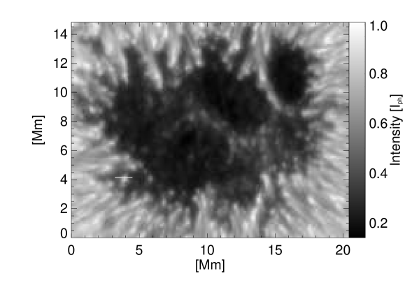
Abbildung 6.1: Continuum intensity map of the sunspot NOAA 10933 as observed by the Hinode SOT/SP on 2007 January 5. Heliocentric angle is $\theta$ = 4^∘. Intensities are normalized to the intensity level of the quiet photosphere $I_{ph}$. The white line at (4,4) Mm marks the cut through an umbral dot (UD) that is discussed in greater detail.

6.3 Data analysis

To obtain atmospheric stratifications of temperature ($T$), magnetic field strength ($B$), and line-of-sight velocity ($v_{LOS}$) we use the inversion code SPINOR described by Frutiger et al. (2000). This code incorporates the STOPRO routines (Solanki, 1987), which compute synthetic Stokes profiles of one or more lines upon input of their atomic data and one or more model atmospheres. Local thermodynamic equilibrium conditions are assumed and the Unno-Rachkovsky radiative transfer equations are solved. The inversions use an optical depth scale as the appropriate coordinate for radiative transfer problems. For reasons of comparability we use the optical depth at 500 nm ($\tau_{500}$). Starting with an initial guess model, the synthetic profiles were iteratively fitted to observed data using response functions (RFs) and the merit function $\chi^{2}$ (Ruiz Cobo & del Toro Iniesta, 1992; Frutiger, 2000) is minimized. With the help of the RFs we find that the Fe I line pair at 6302 Å is mainly formed within the $\log(\tau_{500})$ interval [$-3,0$], which corresponds to a height range of about 400 km under hydrostatic equilibrium conditions in the umbra. The free parameters are defined at the four nodes $-3$, $-2$, $-1$, and $0$ of the $\log(\tau_{500})$ grid. The atmospheric stratification is then interpolated using splines onto a 10 times finer $\log(\tau_{500})$ grid.

The first step of our analysis is the wavelength calibration required to determine line-of-sight (LOS) velocities. For every slit position we average the Stokes $I$ profiles of all locations along the slit whose total polarization $P=\int(Q^{2}+U^{2}+V^{2})^{1/2}d\lambda$ is negligible, since those locations are assumed to represent the quiet Sun. This mean $I$ profile is used to fit Voigt profiles to the two Fe I lines from which the line center wavelengths are determined. The convective blueshift of 140 m s^-1 (see Martínez Pillet et al., 1997; Dravins et al., 1981) is then removed.

The next step is to find an appropriate model atmosphere. Since we are interested in the atmospheric stratification of temperature, magnetic field strength, and LOS velocity within a UD, these three atmospheric parameters are assumed to be height dependent, whereas field inclination and azimuth angle, micro-turbulence, and macro-turbulence are assumed to be height independent. We experimented intensively with adding a second model component to represent the stray light, but the inversion results did not improve significantly, confirming the almost negligible stray light in the SP. Therefore, in the interests of a robust inversion, we forbore from adding a stray light component, thus reducing the number of free parameters.

Lastly, we have to find initial guesses for all free parameters. We use an initial temperature stratification according to the umbral core model L of Maltby et al. (1986) and assume a vertical magnetic field of 2000 G and zero LOS velocity at all heights. Initial guesses for micro-turbulence and macro-turbulence are 0.1 and 2 km s^-1, respectively. Other initial guesses gave very similar results, except for a limited number of outliers. For these, repeating the inversion with an initial guess close to the final result of one of the neighboring pixels returned values consistent with those obtained for the other pixels.

6.4 Inversion results

We analyzed a total of 51 UDs, which were identified by applying the multilevel tracking (MLT) algorithm (Bovelet & Wiehr, 2001; Riethmüller et al., 2008d). For each UD the location of its core was identified, a cut was made through it, reaching to the neighboring diffuse background (DB), and the profiles from all the pixels along this cut were inverted. We first discuss the results for the UD marked in Fig. 6.1, chosen because of its brightness, which leads to particularly small error bars. A comparison of the measured profiles with the best-fit profiles resulted from the inversion can be seen in Fig. 6.2 for the UD and in Fig. 6.3 for the DB selected as the location of lowest continuum intensity in a 1.4 $\times$ 1.4 Mm² environment of the UD center. Due to the low signal in the dark background the measured DB profiles are much noisier than the UD center’s profiles, but in general, the Stokes spectra can be fitted remarkably well.

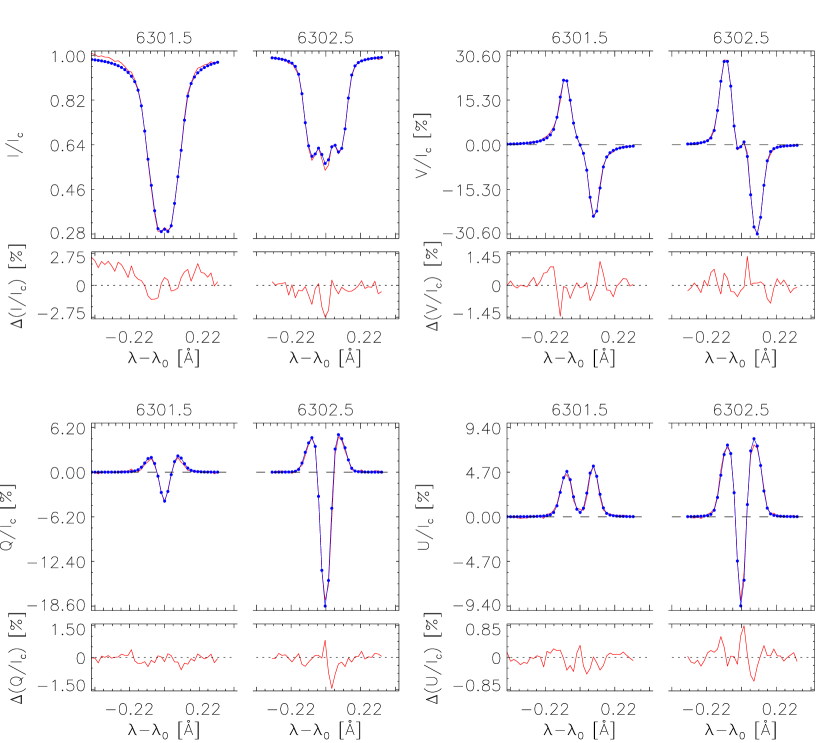
Abbildung 6.2: Stokes $I$, $V$, $Q$ and $U$ profiles from the center of the UD marked in Fig. 6.1. Red lines are the measured, blue lines the best-fit profiles, i.e. the inversion result. The bottom parts of each panel show the difference between the two on an expanded scale.

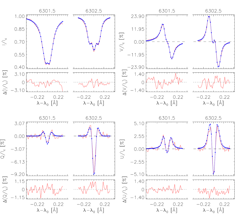
Abbildung 6.3: The same as Fig. 6.2, but for Stokes $I$, $V$, $Q$ and $U$ profiles of the diffuse background near the UD.

The stratification of the retrieved atmospheric parameters $T$, $v_{LOS}$, and $B$ in the center of the UD and in the DB are plotted in Fig. 6.4. In the upper photosphere ($-3\leq\log(\tau_{500})\leq-2$) the error bars overlap; i.e. we find little significant difference between UD and DB. In the deeper photosphere, however, the inversions return strongly different stratifications. Thus, the UD temperature is higher than the DB temperature, consistent with the intensity enhancement of the UD in the continuum map. The LOS velocity (which is identical to the vertical velocity due to the small heliocentric angle) exhibits strong upflows in the UD center, whereas the DB is nearly at rest. The magnetic field strength is roughly 2 kG for the heights $-3\leq\log(\tau_{500})\leq-1$. Below $\log(\tau_{500})=-1$ the field strength of the UD decreases strongly with depth, whereas the field strength of the DB increases moderately.

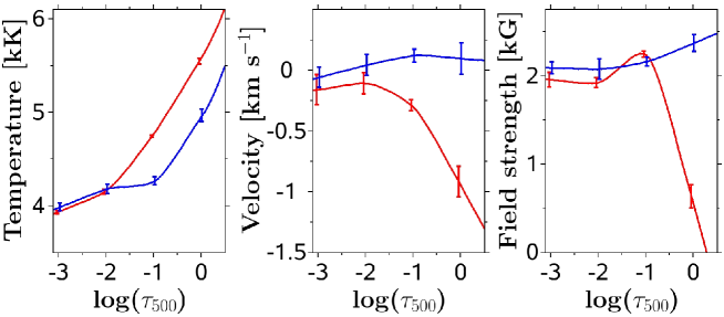
Abbildung 6.4: Atmospheric stratification obtained from the Stokes profiles at the location of the UD’s center (red lines) and from the Stokes profiles of the diffuse background near the UD (blue lines). The formal errors of the inversion at the used optical depth nodes are indicated by bars. Negative LOS velocity values indicate upflows.

The vertical cuts of magnetic field strength and LOS velocity through 13 pixels lying along the white line in Fig. 6.1 are shown in Fig. 6.5. Jumps from one pixel to the next were smoothed through interpolation. There is clear evidence for a localized decrease in UD field strength in the low photosphere, co-located with an upflow that extends higher into the atmosphere and a weak downflow on at least one side. The magnetic fields are 4^∘ more inclined in the UD than they are in the DB around the UD. Fig. 6.5 looks remarkably like Fig. 2 of Schüssler & Vögler (2006), in spite of the fact that Fig. 6.5 is plotted on an optical depth scale in the vertical direction and is thus distorted by an unknown amount relative to a corresponding figure on a geometrical scale.

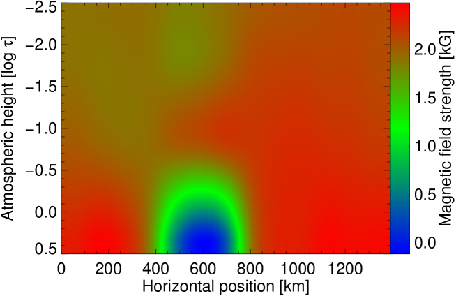
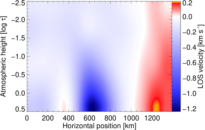
Abbildung 6.5: Vertical cut through the UD marked in Fig. 6.1 in the direction indicated by the white line. Colors of the top panel indicate magnetic field strength. The bottom panel shows LOS velocity. Negative velocities are upflows.

Next we discuss all 51 analyzed UDs. In the literature we often find a separation into two UD regimes. For example, Grossmann-Doerth et al. (1986) differentiate between peripheral UDs (PUDs) and central UDs (CUDs), i.e. between UDs that are born close to the umbra-penumbra boundary and UDs that are born deep in the umbra. We follow this distinction and plot the obtained stratifications of the 30 PUDs (distance to umbra-penumbra boundary less than 2000 km) in the top panels of Fig. 6.6, while the remaining 21 CUDs are represented in the bottom panels of Fig. 6.6. The results largely mirror those obtained for the UD discussed above. In the upper atmosphere UDs center and DB do not differ in their mean values of $T$, $v_{LOS}$, and $B$. On average, the CUDs are about 150 K cooler than the PUDs in the upper atmosphere, just as the DB around the CUDs is cooler than the DB around the PUDs. At $\log(\tau_{500})=0$ we find that PUDs are 570 K hotter than the local DB and CUDs are 550 K hotter than the DB in their vicinity. The magnetic field strength at $\log(\tau_{500})=0$ is weakened by about 510 G for PUDs and 480 G for CUDs, whereas only PUDs exhibit significant upflows of about 800 m s^-1. The mean LOS velocity shows no difference between CUD centers and DB. In order to make sure that an upflow is not being missed due to the lower S/N ratio of the CUD Stokes profiles, we have also averaged the Stokes profiles of all the CUDs. An inversion of there averaged Stokes profiles gave a result that agrees with the averaged stratifications ($green\leavevmode\nobreak\ line$) in the bottom panels of Fig. 6.6 within the error bars. This suggests that any upflow velocity in CUDs is mostly restricted to layers below the surface or is too concentrated or too weak to be detected by the inversions. Finally, we find that the magnetic field of the PUDs is on average 4^∘ more horizontal than for their DB. We see no inclination difference for CUDs.

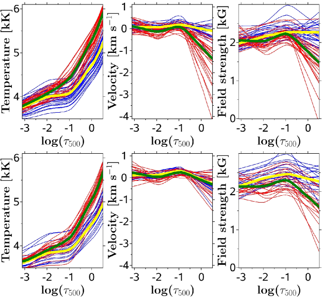
Abbildung 6.6: Atmospheric stratifications of peripheral umbral dots (top 3 panels) and central umbral dots (bottom 3 panels). The red lines show the stratification at the location of the UD’s center and the blue lines correspond to the nearby diffuse background. The green line is the weighted average of all red lines and the yellow line is the weighted average of all blue lines, where we used the reciprocal error bars as weighting factors.

6.5 Discussion

We identified 30 peripheral and 21 central umbral dots in Hinode spectropolarimetric data of a sunspot within 4^∘ of disk center. With the help of Stokes profile inversions of the Fe I lines at 630 nm we determined the stratifications of temperature, magnetic field strength, and LOS velocity. The present work differs from that of Socas-Navarro et al. (2004) in the superior quality of the employed data with twice the spatial resolution and practically no scattered light. This allows a detailed determination of the atmospheric stratification. The higher spatial resolution of the Hinode SP data also allows us to, for the first time, reconstruct both the horizontal and the vertical structure of UDs. We also extended the analysis to a more numerous statistical ensemble of 51 UDs.

Vertical cuts through UDs provide a remarkable confirmation of the results of MHD simulations of Schüssler & Vögler (2006): both show that UDs differ from their surroundings mainly in the lowest visible layers, where the temperature is enhanced and the magnetic field is weakened. We found a temperature enhancement of 550 K and a magnetic field reduction of about 500 G (at optical depth unity). In addition, PUDs display upflow velocities of 800 m s^-1 on average, again in good agreement with the simulations. There are also some differences between our results and those of Schüssler & Vögler (2006). Thus, according to our inversions the magnetic field strength of the DB is somewhat depth dependent. This was not the case for the MHD simulations due to the used periodic boundary conditions. Furthermore, although some of the UDs display a weak downflow bounding the strong central upflow (see Fig. 6.5), these are neither as narrow nor as strong as the downflows at the ends of dark lanes as reported by Schüssler & Vögler (2006), probably due to the limited spatial resolution of our data. We may also be missing some of the narrow downflows by considering only single cuts across individual UDs.

Socas-Navarro et al. (2004) reported 10^∘ more inclined magnetic fields in PUDs. This result is qualitatively confirmed by our work; we find an inclination increase of 4^∘ for PUDs but no increase for CUDs, which can be assumed as a further hint that the main part of the CUD structure is below the surface. These results can be interpreted in terms of the strong DB fields expanding with height and closing over the UD, as proposed by Socas-Navarro et al. (2004).

Kapitel 7 Vertical flows and mass flux balance of sunspot umbral dots¹

7.1 Introduction

Umbral dots (UDs) are small brightness enhancements in sunspot umbrae or pores and were first detected by Chevalier (1916a). The strong vertical magnetic field in umbrae suppresses the energy transport by convection (Biermann, 1941), but some form of remaining heat transport is needed to explain the observed umbral brightness (Adjabshirzadeh & Koutchmy, 1983). Magnetoconvection in umbral fine structure, such as UDs and light bridges, is thought to be the main contributor to the energy transport in the umbra (Weiss, 2002), see reviews by Solanki (2003); Sobotka (2006); Borrero & Ichimoto (2011).

Progress in the physical understanding of umbral dots was made by the numerical simulations of three-dimensional radiative magnetoconvection (Schüssler & Vögler, 2006; Bharti et al., 2010). Most of the simulated UDs have a horizontally elongated shape and show a central dark lane in their bolometric intensity images. In the deepest photospheric layers, the inner parts of UDs exhibit magnetic field weakenings and upflow velocities. The simulated UDs are surrounded by downflows that are often concentrated in narrow downflow channels at the endpoints of the dark lanes (Schüssler & Vögler, 2006). Higher up in the photosphere, the UDs in the simulations do not differ significantly from the diffuse background.

Considerable efforts on the observational side were made to test these theoretical predictions. Dark lanes inside UDs were found in the observations of Bharti et al. (2007) with the 50 cm Hinode telescope and by Rimmele (2008), who observed with the 76 cm Dunn Solar Telescope. However, Louis et al. (2012) analyzed straylight corrected Hinode/BFI data and did not find dark lanes in their observed UDs, which leaves room for doubt whether the observed phenomena are really identical with the synthetic ones. The UDs described by Bharti et al. (2007) differ from those reported by Schüssler & Vögler (2006) in that the area of the observed features is an order of magnitude larger, possibly they are the remains of a decayed light bridge.

More important than the dark lanes are the flows, since they are central to the convective nature of the UDs. Riethmüller et al. (2008c), using inversions of Hinode/SP data, discovered upflows in the deep layers of peripheral UDs (PUDs) but not in central UDs (CUDs), while downflows were not detected. Later, Ortiz et al. (2010) studied a small pore recorded with the CRISP instrument of the 1 m Swedish Solar Telescope and found irregular and diffuse downflows in the range 500-1000 m/s for a small set of 5 UDs. In contrast, in their recent study, Watanabe et al. (2012) analyzed a larger set of 339 UDs, also observed with CRISP, and found significant UD upflows, but no systematic downflow signals. Thus, the existence of downflows in or around UDs remains uncertain, so that the fate of the material flowing up in UDs is unclear. The depth-dependent inversions of full Stokes profiles done by Socas-Navarro et al. (2004) and later at higher resolution by Riethmüller et al. (2008c) revealed a temperature enhancement and a field weakening for the UDs compared to the nearby umbral background, with both being strongest in the deepest observed layers.

Since the observational picture is inhomogeneous, there is a need for a further UD study with high spatial and spectral resolution being of utmost importance. In this work, the improved Stokes inversion method of van Noort (2012) is applied to Hinode/SP data (see van Noort et al., 2013). This so-called 2D inversion method allows the depth-dependent structure to be obtained basically as it would be in the absence of the telescope’s point spread function (PSF).

7.2 Observation, data reduction, and analysis

The data we analyzed in this study were recorded from 12:43 to 13:00 UT on 2007 January 5 with the spectropolarimeter (SP, Lites et al., 2001) of the Solar Optical Telescope (SOT, Tsuneta et al., 2008) on the Hinode spacecraft (Kosugi et al., 2007). SP was operated in its normal map mode, i.e. the integration time per slit position was 4.8 s, resulting in a noise level of $10^{-3}$ (in units of the continuum intensity). The sampling along the slit, the slit width as well as the scanning step size were 0$\mbox{.}^{\prime\prime}$16, the spectral sampling in the considered range from 6300.89 to 6303.26 Å was 21 mÅ pixel^-1. The center of the observed umbra was located very close to the disk center, at a heliocentric angle of 2.6^∘. The full Stokes profiles were corrected for dark current as well as flat field effects and calibrated with the $sp\_prep$ routine of the SolarSoft package. Part of the calibrated Stokes $I$ continuum intensity map obtained by Hinode SP is shown in the upper panel of Fig. 7.1. The original FOV is much larger and contains quiet-Sun regions that are used for the intensity normalization.

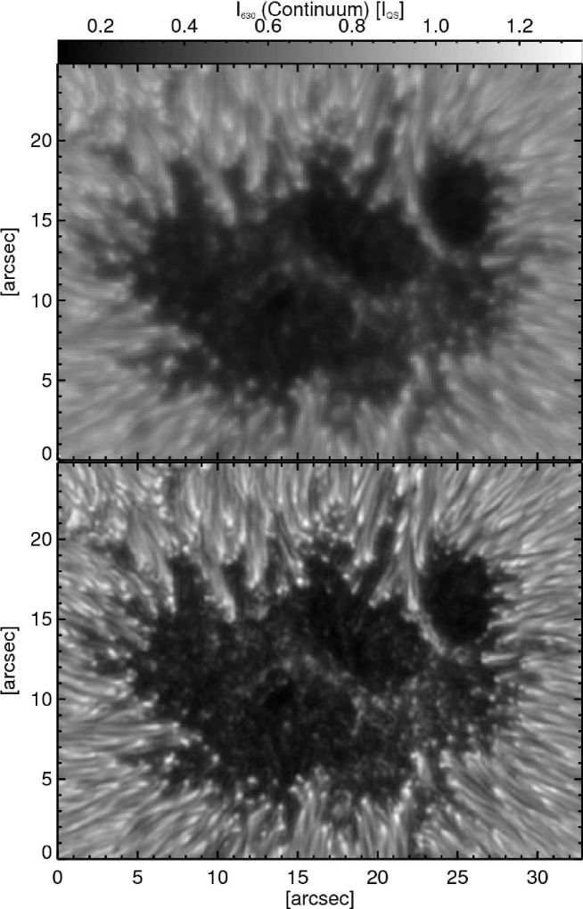
Abbildung 7.1: Stokes $I$ continuum intensity of the Hinode/SP map of a sunspot umbra of NOAA AR 10933 at original resolution (top panel). The Stokes $I$ continuum resulting from the 2D inversion is shown in the bottom panel. The intensity is normalized to the mean quiet-Sun intensity $I_{\rm{QS}}$.

Under the assumption of local thermodynamic equilibrium, the Stokes profiles of the Fe i 6301.5 Å and 6302.5 Å lines were inverted by applying the version of the SPINOR inversion code (Frutiger, 2000; Frutiger et al., 2000) extended by van Noort (2012). In this version of the code, the instrumental effects responsible for the spectral and spatial degradation of the observational data are taken into account, so that the inverted parameters correspond to spatially deconvolved values (but without the added noise that deconvolution generally introduces). The observational data are spatially upsampled by a factor of two, so that the input and output data of the SPINOR inversion have a sampling of 0$\mbox{.}^{\prime\prime}$08 per pixel (for details, see van Noort et al., 2013). The spatial PSF used by the code is taken from Danilovic et al. (2008) and considers the 0.5 m clear aperture of the SOT, the primary mirror’s central obscuration, the three spiders, and a defocus of 0.1 waves. Height dependent temperature, LOS velocity, magnetic field strength, field inclination, field azimuth, and micro-turbulence are determined at three $\log{\tau_{500}}$ nodes: $-2.5$, $-0.9$, and $0$. More details of the inversion of this spot are provided by van Noort et al. (2013) and Tiwari et al. (2013).

A continuum map obtained from the best-fit Stokes $I$ profiles of the 2D inversion result can be seen in the bottom panel of Fig. 7.1. Since the deconvolution of the data with the theoretical spatial PSF is now indirectly part of the inversion process, the contrast is significantly enhanced and umbral dots can be identified much more clearly than in the original data. Hence, the continuum map in the bottom panel of Fig. 7.1 is used for a manual detection of the location of the most prominent 81 UDs which we divided into 25 central UDs (CUDs) and 56 peripheral UDs (PUDs) depending on their distance to the umbra-penumbra boundary. Once the locations of the UDs’ centers are known, the UD boundaries are determined from the continuum map by a multilevel tracking (MLT) algorithm (see Bovelet & Wiehr, 2001), using 25 equidistant intensity levels. The resulting contiguous MLT structures are then cut at 50% of the local min-max intensity range, which is taken as the UD boundary. A detailed description of the use of the MLT algorithm for isolating UDs is given by Riethmüller et al. (2008d).

The knowledge of the UD boundaries allowed us to average UD properties over all pixels within the UD boundary. Stratifications of temperature, LOS velocity, and field strength of the UDs were then determined as such averages. The same quantities were also determined for the UDs’ diffuse background (DB), defined as the average over all pixels in a 400 km wide ring around the UD boundary. UD and DB quantities were retrieved for optical depths between $\log{\tau_{500}}=-2.5$ and 0 in steps of $0.5$.

The LOS velocity maps of the inversion result show a clear $p$-mode pattern with a spatial wavelength of about 10^′′ that has to be removed to avoid any $p$-mode influence on our results. The usually employed technique of Fourier filtering in three-dimensional $k\omega$-space cannot be applied in our case because only a single map of the observational data was available for inversion. We therefore removed the $p$-modes in the LOS velocity maps at all used $\log{\tau_{500}}$ nodes by applying a highpass filter (implemented as the difference between the original velocity map and its running boxcar, $21\times{}21$ pixels, filtered counterpart). Since our results depend on a careful zero velocity determination, we re-calibrated the velocities even if the highpass filter already roughly removed the velocity offset. To achieve this we assume that the dark core of the umbra is at rest. The darker part of the umbra is identified by thresholding the lowpass filtered continuum image ($11\times{}11$ pixels) at 50% of the intensity range. We further excluded a circle of 600 km radius around each of the 81 identified UDs and subtracted the mean velocity of the remaining dark umbral pixels from the velocity maps at each optical depth. This procedure was found to be robust in the sense that changing the threshold for identifying the darkest part of the umbra by $\pm 10\%$, or increasing the radius of the exclusion zone around the UDs by 200 km did not influence our results.

7.3 Results

Even at the significantly improved image quality provided by the inversion, we were not able to find dark lanes in the central parts of the UDs as reported by Schüssler & Vögler (2006) in MHD simulations and by Bharti et al. (2007) in other deconvolved Hinode images.

The stratifications of temperature, velocity, and field strength, averaged separately over all PUDs and CUDs, are displayed in Fig. 7.2. While in the upper photosphere ($\log{\tau_{500}}=-2.5$) the considered properties hardly differ between the mean UD and DB, they deviate significantly from each other in the deep photosphere ($\log{\tau_{500}}=0$). Compared to their DB we find at optical depth unity a temperature enhancement and a field weakening of 760 K and 770 G, respectively, for the mean PUD, while for CUD the values are 540 K and 540 G. The mean UD magnetic field weakens with depth and the weakening in PUDs is more enhanced than the one in CUDs. The field strength of the mean DB increases with depth, as expected.

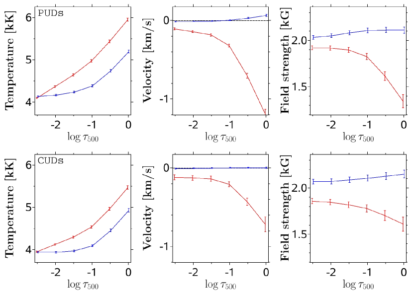
Abbildung 7.2: Optical depth dependence of temperature, LOS velocity, and magnetic field strength averaged over 56 peripheral umbral dots (top 3 panels) and 25 central umbral dots (bottom 3 panels). The error bars denote standard deviations of the mean ($\sigma/\sqrt{N}$). The red lines exhibit the stratifications of the mean UD while the blue lines correspond to the mean nearby diffuse background (see main text for details). Negative LOS velocity values indicate upflows.

The LOS velocity (which is virtually identical to the vertical velocity component due to the small heliocentric angle) of DB and UD is almost zero in the upper photosphere. Strong upflows of $-1200$ m/s and $-720$ m/s are found at optical depth unity for the mean PUD and CUD, while a weak but significant downflow of 64 m/s is found for the mean DB of the peripheral UDs only. These values should be compared with the uncertainty in the velocity averaged over the DB of PUDs, $\sigma/\sqrt{N}=14$ m/s ($\sigma$ - standard deviation, $N$ - number of UDs). The DB of the central UDs is on average at rest within the error bars. Further insight into the up- and downflows in and around UDs is given by Fig. 7.3. We averaged the velocities of all pixels at roughly the same distance to the UD center and plotted such mean velocities as a function of the distance to the UD’s center, again separately for PUDs and CUDs. Note that this method is independent of any determination of the UD boundary. Panel (a) of Fig. 7.3 shows the velocities at optical depth unity. Between $0-200$ km distance from the UD’s center, we find upflows. Then, from 200 to 600 km we see downflows (between 200 and 350 km for CUDs), while for distances larger than 600 km the velocity is almost zero. The downflows in the lower photosphere peak at a distance of roughly 220 km from the UD’s center and have values of 110 m/s and 60 m/s for the mean PUD and CUD, respectively. They are thus minute compared to the maximum upflows in the UDs of $-1280$ m/s and $-600$ m/s. Still, the upflows as well as the downflows are on average stronger for the PUDs than for the CUDs. Both up- and downflows increase rapidly with depth (compare the panels (a)-(c)). The upflows within the UDs are much weaker at $\log{\tau_{500}}=-1$ (panel (b)) and the downflows cannot be seen anymore. At $\log{\tau_{500}}=-2.5$ (panel (c)), there is almost no velocity signal at all. The mean intensity profiles are plotted in panel (d) and revealed a half-width-half-maximum radius of 160 km for the PUDs and 140 km for the CUDs.

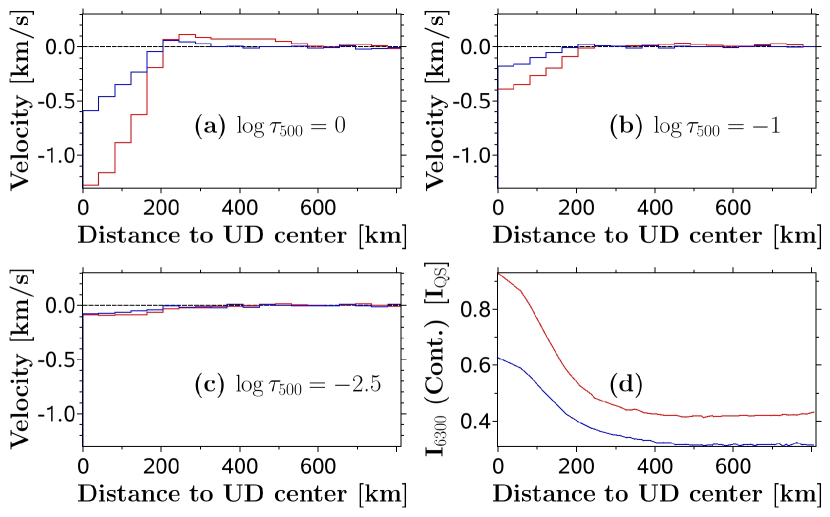
Abbildung 7.3: Panel (a)-(c): LOS velocity at constant optical depth as function of the distance to the UD center averaged over all azimuthal angles of the peripheral (red lines) and central (blue lines) UDs. The optical depths are given as text labels. Panel (d): Mean continuum intensity profile of the two UD classes.

We next calculated mass fluxes as the sum over all pixels within a 600 km vicinity of the UD center since for larger distances the velocity is negligible. The required densities are provided by the SPINOR code under the assumption of hydrostatic equilibrium. Table 7.1 lists the upward and downward mass fluxes per UD, $M_{u}$ and $M_{d}$, for various optical depths and separated for the two UD classes. The uncertainties in Table 7.1 are the standard deviations of the averages over all UDs of a given class ($\sigma$). The last two columns give the mass flux ratios. The mass flux increases strongly with depth due to the density and velocity increase. Even if the downflows are minute compared to the upflows, they cover a much larger area so that the upward and downward mass flux are roughly balanced within the uncertainties.

Tabelle 7.1: Upward and downward mass fluxes per umbral dot (computed within 600 km radii) and their ratios at various optical depths.

$\log{\tau_{500}}$	$M_{u}$	$M_{u}$	$M_{d}$	$M_{d}$	$M_{u}/M_{d}$	$M_{u}/M_{d}$
	PUD	CUD	PUD	CUD	PUD	CUD
	[1O${}^{9}\frac{kg}{s}$]	[1O${}^{9}\frac{kg}{s}$]	[1O${}^{9}\frac{kg}{s}$]	[1O${}^{9}\frac{kg}{s}$]	[]	[]
O	89$\pm$22	75$\pm$13	1O5$\pm$26	69$\pm$1O	O.85$\pm$O.42	1.O9$\pm$O.35
-1	17$\pm$4	22$\pm$4	18$\pm$4	21$\pm$4	O.98$\pm$O.45	1.O2$\pm$O.36
-2	4.6$\pm$1.3	6.O$\pm$1.4	4.1$\pm$1.2	5.5$\pm$1.4	1.12$\pm$O.67	1.1O$\pm$O.52
-2.5	2.5$\pm$O.8	3.3$\pm$O.9	2.2$\pm$O.7	2.9$\pm$O.8	1.17$\pm$O.72	1.14$\pm$O.62

7.4 Discussion and Conclusions

We have used a new inversion technique to retrieve the atmospheric parameters of 81 UDs in a sunspot umbra from data recorded with the spectropolarimeter onboard Hinode. In agreement with earlier studies (Socas-Navarro et al., 2004; Riethmüller et al., 2008c), we find that in the deep photosphere the temperature is enhanced and the magnetic field is weakened in the UDs compared to their umbral surroundings. Table 7.2 compares the main UD properties retrieved from the conventional and the improved inversion technique. For a direct comparison with Riethmüller et al. (2008c), who reported peak values rather than spatial averages, we also give the peak values obtained from the new inversion in Table 7.2. In fact, nearly all values listed in Table 7.2 are higher for the new inversion method, which emphasizes the considerably improved data quality reached by the implicit removal of the telescope’s spatial PSF.

Tabelle 7.2: Comparison of UD properties at the continuum formation height between Riethmüller et al. (2008c) and this study.

UD class	PUD	PUD	PUD	CUD	CUD	CUD
study	2OO8a	this	this	2OO8a	this	this
value type	peak	peak	avg	peak	peak	avg
$T_{\rm{UD}}-T_{\rm{DB}}\,$[K]	57O	112O	76O	55O	79O	54O
$B_{\rm{DB}}-B_{\rm{UD}}\,$[G]	51O	1O2O	77O	48O	72O	54O
$v_{\rm{up}}\,$[m/s]	8OO	224O	128O	-	126O	6OO
$v_{\rm{down}}\,$[m/s]	-	-	11O	-	-	6O

The 2D inversion results revealed clear upflow signals for both UD types, while Riethmüller et al. (2008c) could only find them for the PUDs. On average, UDs show upflows up to a radial distance of 200 km from their centers. In general, these upflows are stronger for PUDs than for CUDs. Between 200 and 600 km from a UD’s center, we find small but significant downflows, whereas there is no relevant velocity signal further away. The velocity signal decreases rapidly with atmospheric height.

Previous observational studies detected upflows, but could not detect downflows associated with UDs (e.g. Socas-Navarro et al., 2004; Riethmüller et al., 2008c; Watanabe et al., 2012), or at least not systematically (Ortiz et al., 2010). This raised the question where all the upflowing plasma ends up. The first systematic detection of downflows around UDs in this paper gives us the possibility of calculating upward and downward mass fluxes. Our finding of rather well-balanced mass fluxes depends on a careful velocity calibration, described in Section 7.2. If all umbral pixels had been used for the zero velocity determination, the zero velocity could possibly be blue-shifted due to the UD upflows, thus giving rise to artificial downflows. This effect is ruled out since our velocity re-calibration ignores the UDs as well as their 600 km surroundings and uses the darkest parts of the umbra only.

We further believe that the downflows seen in the top left panel of Fig. 7.3 are real and not a result of ringing effects. Such effects could be caused by the nearly axisymmetrical shape of the spatial PSF used in our inversion and would have affected all quantities. However, plots of temperature and field strength versus the UD center distance (not shown) do not exhibit any signs of ringing. According to Schüssler & Vögler (2006), the downflows are concentrated in narrow channels preferentially at the endpoints of the central dark lanes of the UDs. Our spatial resolution is insufficient to detect the dark lanes nor the narrow downflow channels. The relatively small downflow signals become significantly larger than the noise only after the azimuthal averaging around UDs.

The picture introduced by Schüssler & Vögler (2006) of UDs as a natural consequence of magnetoconvection in the strong vertical magnetic field of an umbra is confirmed by our study. In deep layers the rising hot plasma pushes the field to the side, weakening the field there. Around the continuum formation height the rising gas cools by radiative losses, turns over, and flows down around the UDs. Such evidence for overturning comes from mass balance between up- and downflows and from the fact that the central upflows are associated with hot material, whereas the peripheral downflows are cool. Furthermore, the rapid decrease of upward mass flux with height is also typical for overturning, overshooting convection. The fact that PUDs are associated with larger flow velocities, greater temperature enhancements, and stronger field reduction suggests a more vigorous convection than in the central umbra.

We suggest observations at a spatial resolution higher than available here, e.g. with the reflight of the 1 m Sunrise telescope (Solanki et al., 2010) or with the 1.5 m Solar-C telescope, to determine if the UDs show the predicted central dark lanes with narrow downflow channels at their endpoints.

Kapitel 8 Bright points in the quiet Sun as observed in the visible and near-UV by the balloon-borne observatory Sunrise¹

8.1 Introduction

Bright points (BPs) are small-scale brightness enhancements located in the darker intergranular lanes. Dunn & Zirker (1973) and Mehltretter (1974) were the first to describe these BPs in filter images taken in the far line wings of H$\alpha$ and Ca ii K, respectively. Common models consider BPs as radiative signatures of magnetic elements, which are often described by nearly vertical slender flux tubes or sheets (Deinzer et al., 1984; Solanki et al., 1993). The increased magnetic pressure within the flux tube leads to its evacuation, and the lateral inflow of heat through the walls of the flux tube makes it hot and bright (Spruit, 1976). Consequently, BPs are often used as tracers of magnetic elements.

The contrast of BPs relative to the average quiet-Sun intensity is of interest since it provides insight into the structure and thermodynamics of magnetic elements. Furthermore, the excess brightness of magnetic elements is an important contributor to variations of the total solar irradiance (Solanki & Fligge, 2002). In the visible, the contrast of BPs is particularly high in wavelength regions that are dominated by absorption bands of temperature-sensitive molecules such as CH and CN (Muller & Roudier, 1984; Berger et al., 1995; Zakharov et al., 2005; Berger et al., 2007; Utz et al., 2009). We expect that their contrast is also large in the ultraviolet (UV), but they have never been studied at wavelengths shorter than 388 nm.

In this work, we extend the study of BPs, in particular their contrasts, to the UV spectral range down to 214 nm, using seeing-free images gathered by the balloon-borne 1-m aperture Sunrise telescope. This is particularly important owing to the finding that irradiance changes below 400 nm produce over 60% of the variation of the total solar irradiance over the solar cycle (Krivova et al., 2006). The spectral and total irradiance variations are caused by the variation of magnetic flux at the solar surface, in particular in the form of small-scale magnetic elements (Krivova et al., 2003, 2006; Wenzler et al., 2006).

8.2 Observations, data reduction, and analysis

The data employed here were acquired during the 2009 June stratospheric flight of Sunrise. Technical details of the telescope are described by Barthol et al. (2011). Image stabilization, feature tracking, and correction of low-order wavefront aberrations were achieved by the gondola’s pointing system in conjunction with a six-element Shack-Hartmann correlating wavefront sensor (Berkefeld et al., 2011).

Observations in the near-ultraviolet spectral domain between 214 nm and 397 nm were acquired with the Sunrise Filter Imager (SuFI, Gandorfer et al., 2011). Simultaneously, the full Stokes magnetograph IMaX (Martínez Pillet et al., 2011) scanned the Fe i line at 525.02 nm (Landé factor $g=3$), hence providing kinematic and magnetic information. An overview of the collected data and a description of some of the observed phenomena is given by Solanki et al. (2010).

We use three time series recorded from 00:36 to 00:59 UT, 01:31 to 02:00 UT, and 14:22 to 15:00 UT on 2009 June 9. At these times, the telescope pointed to quiet regions close to the disk center. The SuFI instrument recorded filtergrams centered at 397 nm (Ca ii H), 388 nm (CN), 312 nm, 300 nm, and 214 nm, while IMaX was operated in its standard vector spectropolarimeter mode, i.e., full Stokes observations at five wavelength points with six accumulations. The five wavelength points were set to $\lambda-\lambda_{0}=-80,-40,+40,+80,$ and $+227$ mÅ relative to the center of the line. A summary of the filter widths (FWHM) and exposure times can be found in Table 8.1. The effective exposure time of an IMaX continuum image was 6 s (6 accumulations $\times$ 4 modulation states $\times$ 250 ms), while Dopplergrams need five wavelength points; i.e., their effective exposure time was 30 s (see Martínez Pillet et al., 2011, for more details).

Tabelle 8.1: Exposure times of the used time series.

Central	FWHM	00:36$-$00:59	01:31$-$02:00	14:22$-$15:00
Wavelength	of Filter	Exp. Time	Exp. Time	Exp. Time
(nm)	(nm)	(ms)	(ms)	(ms)
214	1O	...	...	3OOOO
3OO	5	5OO	5OO	25O
312	1.2	15O	15O	3OO
388	O.8	8O	8O	15O
396.8	O.18	96O	96O	9OO
525.O2	O.OO85	25O	25O	25O

At a typical flight altitude of around 36 km, the 214 nm wavelength range was still strongly attenuated by the residual atmosphere of the Earth, so that an exposure time of 30 s was needed, even at the highest Sun elevations achieved during the flight. The 214 nm data were only acquired during the third time series. The cadence of the IMaX data was always 33 s, while it was 12 s for the SuFI data of the first two time series (i.e., all recorded SuFI wavelengths within 12 s) and it was 39 s for the last time series that included the 214 nm channel.

The data were corrected for dark current and flat field. Additionally, the instrumental polarization was removed from the IMaX data with the help of Mueller matrices determined by pre-flight polarimetric calibrations. Finally, the in-flight phase-diversity measurements (permanently for SuFI and intermittently for IMaX) were used to correct the images for low-order wavefront aberrations (Hirzberger et al., 2011; Martínez Pillet et al., 2011). The phase-diversity reconstruction of the SuFI images was done using averaged wavefront errors (level-3 data, see Hirzberger et al., 2010). All intensity images were normalized to the intensity level of the mean quiet Sun, $I_{\rm{QS}}$, which was defined as the average of the whole image. The images were then re-sampled to the common plate scale of 0$\mbox{.}^{\prime\prime}$0207 pixel^-1 (original plate scale of SuFI’s 300 nm images) via bilinear interpolation, and the common field of view (FOV) of 13^′′$\times$38^′′ was determined. Residual noise was removed by applying a running boxcar filter of 3$\times$3 pixels. Its width corresponds to about half of the spatial resolution of about 0$\mbox{.}^{\prime\prime}$15 reached by the considered observations (determined from radially averaged power spectra). As a proxy of the longitudinal magnetic field, the circular polarization degree $\langle p_{\rm{circ}}\rangle$ averaged over the four points in the line ($-80,-40,+40,+80$ mÅ),

$$\langle p_{\rm{circ}}\rangle=\frac{1}{4}\sum_{i=1}^{4}{a_{i}\frac{V_{i}}{I_{i}}}\leavevmode\nobreak\ ,$$

was calculated with a reversed sign of the two red wavelength points ($\textbf{{a}}=[1,1,-1,-1]$) to avoid cancelation. The line-of-sight (LOS) component of the velocity vector was obtained by a Gaussian fit to the Stokes $I$ profiles. The velocity maps were corrected for the wavelength shift over the FOV caused by the IMaX etalon, and a convective blueshift of 200 m s^-1 was removed (see Martínez Pillet et al., 2011).

Only one set of IMaX and SuFI observations every five minutes was analyzed in order to allow BPs to evolve between images. In total, we analyzed 19 image sets distributed over the three time series. BPs were manually identified in the CN images at 388 nm, in order to be consistent with earlier work that concentrated on visible wavelengths (e.g. Zakharov et al., 2005; Berger et al., 2007). At each of the other wavelengths, we then determined the local brightness maximum in a 11$\times$11 pixel (i.e., 0$\mbox{.}^{\prime\prime}$22$\times$0$\mbox{.}^{\prime\prime}$22) environment of the detected BP position at 388 nm. This method takes into account that the various wavelengths represent different atmospheric layers (most obvious for the Ca ii H images) so that inclined magnetic features may appear at slightly different horizontal positions at different wavelengths. In total, we detected 398 BPs, of which 211 were from the third time series including the 214 nm band.

8.3 Results

Fig. 8.1 shows BPs at 14:27:08 UT in a region of 10^′′$\times$8^′′ (subregion of the 13^′′$\times$38^′′ full FOV). The six upper panels display the five SuFI filtergrams and the IMaX Stokes $I$ continuum image ($+227$ mÅ). Most of the bright features are visible in each filtergram. However, the contrast of these features at 525 nm is significantly lower than in the five shorter wavelengths. Some features show a prominent brightness enhancement in the Ca ii H image but are of moderate brightness at the other wavelengths, e.g., at position (8$\mbox{.}^{\prime\prime}$6, 3$\mbox{.}^{\prime\prime}$8). Most remarkable is the high contrast of the BPs at 214 nm, which strongly exceeds granulation brightness variations. It is this high contrast that lets the granulation appear relatively dark in the first panel of Figure 1, since the gray scales of all panels are adapted to the full min/max range. The bottom left panel shows the LOS component of the velocity. While the three BPs at the positions (1$\mbox{.}^{\prime\prime}$0, 1$\mbox{.}^{\prime\prime}$7), (1$\mbox{.}^{\prime\prime}$8, 0$\mbox{.}^{\prime\prime}$8), and (2$\mbox{.}^{\prime\prime}$6, 1$\mbox{.}^{\prime\prime}$3) show strong downflows of up to 2.5 km s^-1, most other BPs exhibit only moderate velocities. The bottom right panel displays the mean circular polarization degree. Most of the BPs in the plotted region are associated with negative polarity. Nonetheless, several bipolar regions can be seen, for instance the two neighboring BPs at (2$\mbox{.}^{\prime\prime}$3, 7$\mbox{.}^{\prime\prime}$3) and at (2$\mbox{.}^{\prime\prime}$6, 7$\mbox{.}^{\prime\prime}$7), respectively.

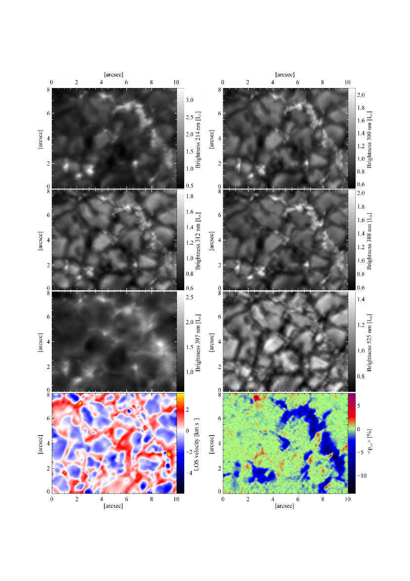
Abbildung 8.1: Intensity maps of the five wavelengths observed by SuFI (two first rows and the left panel of the third one) and of the continuum sample by IMaX (the right panel of the third row), all normalized to the corresponding mean intensity level of the quiet Sun, $I_{\rm{QS}}$. The LOS velocity obtained from a Gaussian fit (positive velocities correspond to downflows) and the mean circular polarization degree (see the main text for definition) are shown in the bottom panels.

Histograms of the BP peak intensity relative to the mean quiet-Sun intensity are displayed in Fig. 8.2 as red lines in panels (a)$-$(f). The blue lines correspond to the brightness histograms of the darkest pixel whose distance to a BP’s brightest pixel is less than 0$\mbox{.}^{\prime\prime}$3 (typical width of an intergranular lane). The text labels denote the mean values. The red histograms are largely symmetric, although there is a tendency for a tail toward higher contrast values, in particular at 214 nm and 397 nm. As already indicated in Fig. 8.1, the largest average contrast is shown by BPs in the 214 nm image. The highest peak brightness of 5.0 $I_{\rm{QS}}$ is also reached at this wavelength. At first sight it might be surprising that some BPs are less bright than some of the pixels of the blue histograms. A closer look reveals, however, that all BPs are indeed bright relative to the pixels in their immediate surroundings. For the Ca ii H line, the mean intensity of the darkest pixels in the BPs’ vicinity is, with 1.07 $I_{\rm{QS}}$, higher than for the other wavelengths, because the Ca structures are generally more diffuse and larger than our limit of 0$\mbox{.}^{\prime\prime}$3. The green curves give histograms of the normalized intensity for all pixels in all frames, practically representing the intensity distribution of quiet-Sun granulation. A comparison of the maximum position of the red and green histograms clearly shows that the BPs are much more conspicuous in the UV than in the visible spectral range. The quiet-Sun histograms are more extended toward higher intensities than the histograms for the BP background, since the latter largely represents intergranular lanes. Exceptions are the histograms for Ca ii H, which shows reverse granulation and those for 214 nm, where the comparable width indicates structures intermediate between reverse and normal granulation (see Solanki et al., 2010).

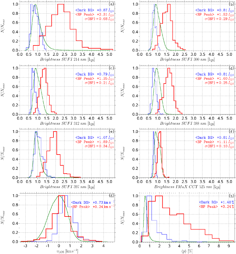
Abbildung 8.2: Brightness histograms of the six wavelengths observed by Sunrise together with histograms of the LOS velocity and the averaged polarization degree. Red lines correspond to histograms of the BPs’ brightest pixel, blue lines to the darkest pixel in a 0$\mbox{.}^{\prime\prime}$3 vicinity of the bright point, and the green lines denote histograms of all pixels in all frames. The mean values of the red and blue histograms as well as the standard deviations of the red brightness histograms are indicated as the text labels.

Panel (g) of Fig. 8.2 shows the LOS velocity histograms for the brightest BP pixels (red), the darkest pixels of their vicinity (blue), and for all pixels (green). On average, the LOS velocity of the darkest pixels shows a downflow of 730 m s^-1, while the BPs themselves are associated with a clearly weaker average downflow of 240 m s^-1. However, the broad wings of the distribution contain BPs with significant upflows of up to $-3.1$ km s^-1 or downflows of up to 3.6 km s^-1. 7.5% of the analyzed BPs have upflows with $v_{\rm{LOS}}<-1$ km s^-1 and 15% of the BPs show downflows with $v_{\rm{LOS}}>1$ km s^-1. The red histogram (BP velocities) is located between the green histogram (dominated by the large number of pixels showing upflows) and the blue histogram (mainly intergranular pixels showing downflows). Our velocities are obtained from a Gaussian fit to the Stokes $I$ profiles. The Stokes $V$ zero-crossings may possibly show different velocities if a BP is not spatially resolved.

In contrast to the last panel of Fig. 8.1, where the signed net circular polarization was plotted, panel (h) of Fig. 8.2 displays the histogram of the unsigned total polarization degree $\langle p\rangle$ averaged over the four wavelength points in the Fe i line,

$$\langle p\rangle=\frac{1}{4}\sum_{i=1}^{4}{\sqrt{\left(\frac{Q_{i}}{I_{i}}\right)^{2}+\left(\frac{U_{i}}{I_{i}}\right)^{2}+\left(\frac{V_{i}}{I_{i}}\right)^{2}}}\leavevmode\nobreak\ .$$

This histogram is highly asymmetric. The polarization degree at the positions of the peak brightness reaches values of up to 9.1%, the mean value is 3.24%. Such large values of the polarization in 525.02 nm suggest that at least some of the magnetic features have been resolved (see Lagg et al., 2010, for more details). However, 4.3% of the BPs are associated with $\langle p\rangle<1\%$. Although the polarization degree in the darkest surrounding pixels is weaker, almost all of them still show a significant polarization degree of more than $0.3\%$ (three times the noise level) with the strongest value being 6.6%. Polarization usually displays larger structures than the BPs (see the bottom right panel of Fig. 8.1 and Title & Berger, 1996), which can also be concluded from the fact that the blue histogram shows larger polarization values than the green histogram for all pixels.

The mean values and their standard deviations for all red and blue histograms in Fig. 8.2 are summarized in Table 8.2. Columns labeled with BP refer to histograms of the BP peak value, while DB denotes the histograms of the dark background. The standard deviation of the BP brightness is $\approx 0.5\left(\left\langle I/I_{\rm{QS}}\right\rangle-1\right)$ in all the SuFI channels, except Ca ii H. This relationship can be used to estimate the brightness histogram width for other wavelengths. The rightmost column of the table shows the ratio of the BP contrast (mean BP brightness value minus one) to the rms intensity contrast (taken from Hirzberger et al., 2010, and calculated over the whole FOV of the level-3 data). This contrast is a measure of how strongly BPs stand out relative to the surrounding granulation (or reversed granulation and waves in the case of 397 nm). According to Table 8.2, images at 214 nm show the BPs most clearly.

Tabelle 8.2: Bright point histogram properties.

Quantity	Mean	$\sigma$	Mean	$\sigma$	Contrast
	BP	BP	DB	DB	Ratio
$\left(I/I_{\rm{QS}}\right)_{214}$	2.31	O.68	O.87	O.21	4.7
$\left(I/I_{\rm{QS}}\right)_{3OO}$	1.52	O.29	O.81	O.11	2.4
$\left(I/I_{\rm{QS}}\right)_{312}$	1.35	O.21	O.79	O.1O	1.8
$\left(I/I_{\rm{QS}}\right)_{388}$	1.6O	O.25	O.81	O.11	3.3
$\left(I/I_{\rm{QS}}\right)_{397}$	1.89	O.34	1.O7	O.2O	4.O
$\left(I/I_{\rm{QS}}\right)_{525}$	1.11	O.1O	O.81	O.O6	O.8
$v_{\rm{LOS}}\,(\rm{m\,s^{-1}})$	24O	91O	73O	65O
$\langle p\rangle\,(\rm{\%})$	3.24	1.82	1.4O	O.84

8.4 Summary and discussion

We identified 398 BPs in simultaneously observed photometric and polarimetric Sunrise images of a quiet-Sun region close to the disk center. Our data include three wavelengths in the near-UV in which the Sun was never observed before at high spatial resolution. We determined the peak brightness and the brightness of the dark background of every detected BP at each observed wavelength. The BPs’ peak intensity reaches up to 5.0 times the mean quiet-Sun intensity $I_{\rm{QS}}$ at 214 nm. The mean peak intensity at that wavelength is 2.31 $I_{\rm{QS}}$. The 214 nm wavelength also displays the largest ratio of BP contrast to the rms of the intensity over the whole FOV (see the rightmost column of Table 8.2). This ratio is a measure of how prominent BPs are in an image at a particular wavelength. These values indicate that they are even more prominent at 214 nm than in the core of Ca ii H (for the 0.18 nm wide filter employed by SuFI).

The value of the mean peak brightness at 388 nm (1.60 $I_{\rm{QS}}$) agrees exactly with the CN peak brightness obtained by Zakharov et al. (2005) from data recorded with the 1 m Swedish Solar Telescope (SST). Examples of BP brightness values (close to the disk center) given in the literature for the frequently observed $G$-band at 430 nm (CH molecule) are 1.45 $I_{\rm{QS}}$ (Zakharov et al., 2005) and 1.2 $I_{\rm{QS}}$ (Berger et al., 2007). Both studies analyzed SST data. Utz et al. (2009) used $G$-band data from the 50 cm Solar Optical Telescope onboard Hinode and found 1.3 $I_{\rm{QS}}$. These values are comparable with what we find in the near-UV, with the exception of 214 nm, which displays distinctly higher values. Note that the BP contrasts given in this study are not corrected for instrumental scattered light. After this correction, the BP contrasts will most likely increase (see, e.g., Feller et al., in preparation; Wedemeyer-Böhm, 2008; Mathew et al., 2009).

From the spectropolarimetric data we derived the LOS component of the velocity vector. The largest BP velocities reach $-3.1$ km s^-1 in upflows and 3.6 km s^-1 in downflows. The mean value is 240 m s^-1, in good agreement with the average velocity of 260 m s^-1 published by Beck et al. (2007) and reasonably consistent with the absence of Stokes $V$ zero-crossing shifts found by Solanki (1986) and Martínez Pillet et al. (1997) in data with much lower spatial resolution. In contrast to this, Grossmann-Doerth et al. (1996) reported a stronger mean downflow of 800 m s^-1 as derived from the zero-crossing of their Stokes $V$ profiles and Sigwarth et al. (1999) found a velocity range of $\pm$5 km s^-1 and a mean velocity of 500 m s^-1. The nature of the BPs displaying strong up- or downflows in Stokes $I$ will be investigated in a subsequent study.

The polarization degree, averaged over the four points within the Fe i line, is also calculated from the IMaX data and shows values up to 9.1%. The mean BP polarization degree is 3.24%, which is clearly above the mean signal of 1.40% for the dark vicinity. Intriguingly, about 4% of the BPs are associated with relatively weak magnetic flux ($\langle p\rangle<1\%$). This raises interesting questions, since enhanced temperatures and hence brightness in magnetic elements (flux tubes) is caused by evacuation, which in turn is proportional to $B^{2}$. Therefore, we would expect that BPs show strong Stokes $V$ signals. Significantly inclined magnetic fields cannot explain the observed weak Stokes $V$ signals, because we also measured weak Stokes $Q$ and $U$ signals. Additionally, strongly evacuated flux tubes are strongly buoyant and hence should be nearly vertical (Schüssler, 1986). Lagg et al. (2010) find a strong Stokes $I$ line weakening for kilo-Gauss network patches due to temperature enhancements in the flux tubes. Such an absorption weakening can also lead to a weak Stokes $V$ signal. Although the network patches analyzed by Lagg et al. (2010) are spatially resolved, we find many BPs that exhibit complex Stokes profiles, which is a clear indication that not all of the BPs are spatially resolved. Insufficient resolution can also contribute to weak Stokes $V$ signals.

In summary, we find high intensity contrasts of BPs in the near-UV range (including the first measurements below 388 nm), with values up to 5 $I_{\rm{QS}}$ at 214 nm. The simultaneous spectropolarimetric measurements confirm the close association of BPs with magnetic flux concentrations in intergranular downflow lanes. However, the majority of the BPs exhibit only weak downflows.

The reasonably high cadence of Sunrise data (between 4 s and 39 s, depending on the number of observed wavelengths and their exposure times) and the high measured contrasts of BPs make detailed future studies of the dynamical properties of BPs very promising (e.g., Jafarzadeh et al., 2013). Of considerable additional benefit for such studies will be the possibility to compare the dynamics at different layers in the solar atmosphere, which are covered by the combination of SuFI and IMaX wavelength bands.

Kapitel 9 Comparison of solar photospheric bright points between Sunrise observations and MHD simulations¹

9.1 Introduction

Magnetic fields in the network and in active region plage are often concentrated into strong kilo-Gauss field elements (Stenflo, 1973; Solanki et al., 2006; Ishikawa et al., 2007). At high spatial resolution such elements appear as bright points (BPs, Berger & Title, 2001) owing to the inflow of radiation from their walls into their evacuated interiors (Spruit, 1976; Deinzer et al., 1984). Many features of magnetic elements are known (see Solanki, 1993, for an overview) and various aspects of the underlying model of magnetic flux tubes have been tested, but such tests have generally suffered from the fact that the data were not able to spatially resolve magnetic elements.

This situation has changed with the availability of data recorded by the Sunrise balloon-borne observatory, which have allowed magnetic elements even in the internetwork quiet Sun to be spatially resolved (Lagg et al., 2010). Hence, it is now a good opportunity to revisit BPs and to compare their observational properties with predictions from state-of-the-art radiation MHD simulations.

One motivation to study BPs is their contribution to variations of the total solar irradiance (TSI). Around the maximum of the solar activity cycle, the reduction of solar irradiance owing to dark sunspots and pores is overcompensated by an increased brightness of the BPs (Fröhlich, 2011). As a result, TSI, i.e. the irradiance integrated over all wavelengths, is on average higher during the solar maximum than during minimum (Willson & Hudson, 1988). The TSI variations are only weak over the solar cycle, but because 60 % (Krivova et al., 2006) or even more (Harder et al., 2009) of the variations in TSI are produced at wavelengths shorter than 4000 Å, the variations in the ultraviolet (UV) can be much more relevant. From recent stratospheric observations we know that the BP contrasts are particularly high in the UV (Riethmüller et al., 2010), i.e. the radiative properties of BPs possibly play an important role in influencing the Earth’s climate. A variation of the UV irradiance changes the chemistry of the stratosphere, which can propagate into the troposphere and finally influence the climate (London, 1994; Larkin et al., 2000; Haigh et al., 2010; Gray et al., 2010; Ermolli et al., 2012).

In addition, there are reasons intrinsic to solar physics why BPs are of interest. Firstly, BPs are the most easily visible signatures of strong-field magnetic elements and hence have been widely observed (e.g. Muller & Roudier, 1984; Berger et al., 1995; Berger & Title, 2001; Utz et al., 2009). Such magnetic elements carry much of the magnetic energy, even if they harbor only a small fraction of the magnetic flux. Secondly, the flux tubes guide magneto-hydrodynamic waves, which could contribute to coronal heating (Roberts, 1983; Choudhuri et al., 1993) and may be related to the waves found to run along spicules (De Pontieu et al., 2007). Additionally, flux-tube motions can lead to field-line braiding and the build up of energy, which may be released through nanoflares (Parker, 1988).

The first science flight of the Sunrise observatory revealed the very high contrasts of BPs in the UV (Riethmüller et al., 2010). Here we follow up on this work by carrying out a more in-depth analysis of a quiet-Sun region as observed by Sunrise and by comparing the data with numerical simulations of three-dimensional radiative magnetoconvection. Hence we further explore the interplay between observation and simulation which has been so fruitful in the past. The MHD simulation data were degraded with known instrumental effects that were present during the Sunrise observations so that they can be compared directly with the observational data. We extend existing studies by considering many more observational quantities (intensity at multiple wavelengths, line-of-sight (LOS) velocity, spectral line width, and polarization degree) when comparing observational data and MHD simulations, which allowed us to test the realism of the MHD simulations far more stringently than by simply comparing intensities. We carried out such comparisons in two steps, first for all pixels in the images and later restricted to just the pixels identified as lying within BPs. After we satisfied ourselves that the simulations give a reasonable representation of the observations, we used the original, undegraded simulations to learn more about the BPs and their underlying magnetic features.

9.2 Observations, simulations, and degradation

9.2.1 Observations

The data we used in this study were acquired with the balloon-borne 1-m aperture Sunrise telescope that flew from Kiruna in northern Sweden to Somerset Island in northern Canada in June 2009 (Barthol et al., 2011; Solanki et al., 2010). At the flight altitude of roughly 35 km, 99 % of the air mass was below the observatory, so that the disturbing influence of the Earth’s atmosphere (seeing) was minimized. A fast tip-tilt mirror, which was controlled by a correlating wavefront sensor, reduced the residual pointing jitter and the onboard adaptive optics system corrected the images for low order wavefront aberrations (Berkefeld et al., 2011). Two instruments were operated simultaneously: the Sunrise Filter Imager (SuFI; Gandorfer et al., 2011) and the Imaging Magnetograph eXperiment (IMaX; Martínez Pillet et al., 2011).

During the herein considered time series, recorded from 23:00 to 24:00 UT on 2009 June 10, the telescope pointed to a quiet-Sun region close to the center of the solar disk ($\mu=1.0$). SuFI observed the Sun at the wavelengths 2995 Å (33 Å FWHM, 325 ms exposure time, mainly atomic spectral lines), 3118 Å (8.5 Å FWHM, 300 ms exposure time, part of the OH band), 3877 Å (5.6 Å FWHM, 65 ms exposure time, CN band), and 3973 Å (1.8 Å FWHM, 750 ms exposure time, Ca ii H line). Dark current and flat field corrections were applied to the SuFI data. The images were phase-diversity (PD) reconstructed using the wavefront errors retrieved from the in-flight PD measurements via a PD prism in front of the camera. The reconstructed data are referred to as level-2 data, see Hirzberger et al. (2010, 2011). Here we concentrated on the 3118 Å and the 3877 Å bands. The spectra in these bands, taken from the NSO spectral atlas of Kurucz et al. (1984) are plotted in the upper two panels of Fig. 9.1 (black lines) along with the filter profiles (green lines).

IMaX scanned the Fe i line at 5250.2 Å (Landé factor $g=3$) in its L12-2 mode, i.e. only Stokes $I$ and $V$ were measured, at twelve scan positions with two accumulations. The twelve scan positions were set to $\lambda-\lambda_{0}=-192.5,...,+192.5$ mÅ relative to the center of the average quiet-Sun profile of the line, in steps of 35 mÅ. The effective spectral resolution of IMaX was 85 mÅ (full-width-half-maximum (FWHM) value). The data were corrected for dark current and flat field and interference fringes were removed with a manually designed Fourier filter. The IMaX data were then reconstructed with the help of the phase diversity technique. Additionally, the instrumental polarization and the residual cross-talk with intensity was removed. Stray light was not removed from either data set. All intensity images were divided by the mean quiet-Sun value, $I_{\rm{QS}}$, that was defined as the average of the image.

Finally, the Stokes $I$ profiles were fitted with a Gaussian function to retrieve the spectral line parameters: LOS velocity and line width. The increased reliability of the retrieved parameters for more scanned line positions was the main driver for using data with twelve scan positions instead of five as in the so-called V5-6 mode of IMaX, which was employed in our former study (Riethmüller et al., 2010). Since we were studying BPs, thought to be associated with strong-field, relatively vertical magnetic features, the Stokes $Q$ and $U$ profiles were considered to be less important for the present work. This assumption is supported by the analysis of Jafarzadeh et al. (2013), who found that BPs extend nearly vertically in height. Fig. 9.1 shows relevant parts of the solar spectrum taken from an NSO spectral atlas (Kurucz et al., 1984). The spectrum centered on the Fe i line at 5250.2 Å is plotted in the bottom panel. The simulated profile of the 5250.2 Å line in the presence of an upflow of 5 km s^-1 is overplotted as a dotted red line in order to demonstrate that even strong up- (or downflows) can be safely identified with the L12-2 mode of IMaX (see the blue arrows marking the wavelengths sampled by IMaX in L12-2 mode), but can be missed or missidentified with only five scan positions (see red arrows). The image quality of the Sunrise data was strongly dependent on the gondola’s varying pointing stability. L12-2 data were recorded over only a relatively short period of time during the Sunrise flight, when the pointing stability was not particularly good. Therefore the analyzed L12-2 data have a somewhat worse image quality compared to the better spatially resolved V5-6 data analyzed by Riethmüller et al. (2010). The LOS velocities were corrected for the wavelength shift over the FOV caused by the IMaX etalon (see Martínez Pillet et al., 2011). In this work, negative LOS velocities correspond to upflows.

We selected the nine data sets acquired at 23:05:08, 23:09:20, 23:20:22, 23:26:09, 23:31:56, 23:36:39, 23:42:26, 23:47:09, and 23:53:28 UT for an in-depth study from the one hour time series. The selection was done so that the time interval between two consecutive sets was on average five minutes so as to give the BPs some time to evolve between two analyzed data sets. For each data set we checked that the pointing stability of the gondola and hence the image quality was as good as any among the L12-2 data, although it was found to be somewhat lower than of the best V5-6 data.

9.2.2 Simulations

The three-dimensional non-ideal compressible radiation MHD simulations considered here were calculated with the MURaM code which solves a system of equations consisting of the continuity equation, the momentum equation, the energy equation, the induction equation, and the equation of state (Vögler et al., 2005). The radiative energy exchange rate of the energy equation is determined by a non-gray radiative transfer module under the assumption of local thermal equilibrium (LTE). The equation of state takes into account effects of partial ionization because they influence the efficiency of the convective energy transport. Periodic boundary conditions were used in the horizontal directions. A free in- and outflow of matter was allowed at the bottom boundary of the computational box under the constraint of total mass conservation, while the top boundary was closed (i.e. zero vertical velocity). A statistically relaxed purely hydrodynamical simulation was used as initial condition. From tests with different magnetic fluxes, we estimated the mean unsigned vertical magnetic flux density of our quiet-Sun observations to correspond roughly to a simulation with a starting value of 30 G and hence a unipolar homogeneous vertical magnetic field of $B_{\rm z}=30$ G was introduced into the hydrodynamical simulation (see section 9.3.1 for a more precise estimate of the mean flux). The simulation was run for a further 3 hours of solar time to reach and stay for a sufficiently long time in a statistically stationary state. 30 equidistant snapshots covering 141 min of solar time were then used for this study. The data cubes cover 6 Mm in both horizontal directions with a cell size of 10.42 km (0$\mbox{.}^{\prime\prime}$014). In the vertical direction they extend 1.4 Mm at 14 km cell size. On average, unit optical depth for the continuum at 5000 Å is reached about 500 km below the upper boundary. To evaluate the dependence of our MHD results on the mean magnetic flux, we also calculated 10 snapshots each taken from simulation runs with an initial mean unsigned vertical flux density of 0 G (purely hydrodynamical run), 50 G, and 200 G, while all other parameters were kept identical to the 30 G run.

The output of the MURaM code consisted of data cubes of the density, velocity (x, y, z component), total energy density, magnetic field (x, y, z component) as well as gas pressure and temperature. For a direct comparison with the observations, these quantities had to be converted into Stokes profiles. This was done by a forward calculation with the SPINOR inversion code (Frutiger, 2000; Frutiger et al., 2000; Berdyugina et al., 2003) that uses the STOPRO routines (Solanki, 1987) to compute synthetic Stokes spectra for atomic and molecular spectral lines assuming LTE and solving the Unno-Rachkovsky radiative transfer equations (Rachkovsky, 1962). All spectral line syntheses in this paper were carried out for the center of the solar disk ($\mu=1.0$).

For SuFI’s spectral range at 3118 Å we synthesized 538 spectral lines (spectral sampling was 50 Samples/Å), for the 3877 Å range 354 spectral lines (33 Samples/Å), and finally, for the IMaX instrument we synthesized 20 spectral lines (128 Samples/Å), i.e. the Fe i line at 5250.2 Å itself and 19 of its neighboring lines which could possibly contribute to the synthesized Stokes signals owing to the secondary peaks of IMaX’s spectral point spread function (PSF). For the three considered wavelength ranges, the spatially averaged synthetic spectra (calculated for a snapshot with 30 G average vertical field) are shown in Fig. 9.1 (red lines) and compared with the average observed spectra of quiet Sun taken from the NSO atlas (Kurucz et al., 1984). The synthetic spectra were convolved with a Gaussian of FWHM = 1.93 km s${}^{-1}\sqrt{2/\ln{2}}\leavevmode\nobreak\ \lambda/c$ to fit the spectral resolution of the NSO atlas. The spectral PSF of IMaX (green line in the bottom panel) includes the IMaX prefilter and is plotted on a logarithmic scale for a better visibility of the secondary peaks at 5248.32 Å and 5252.10 Å.

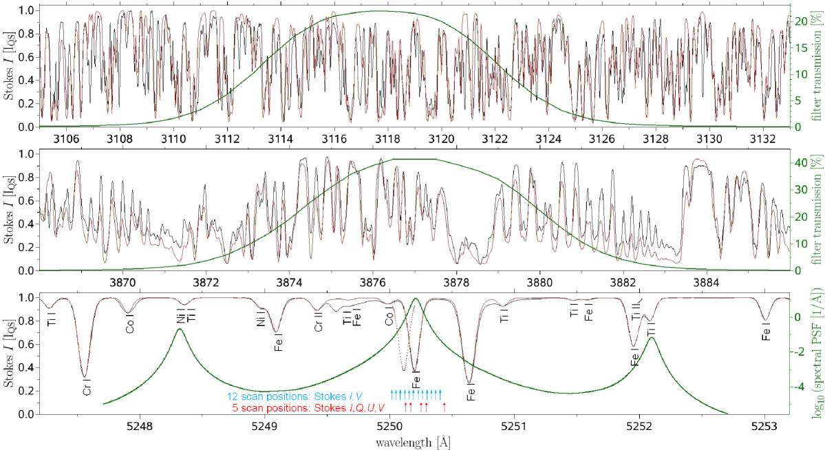
Abbildung 9.1: Excerpts from an NSO spectral atlas (black lines; Kurucz et al., 1984), spatially averaged synthetic spectra (red lines), and instrumental filter profiles (green lines referring to the scale on the right side of the figure) for the part of the OH band around 3118 Å (top panel), the CN band at 3877 Å (middle panel), and the Fe i line at 5250.2 Å (bottom panel). The dotted red line in the bottom panel simulates the Doppler shifted profile of the Fe i line produced by an upflow of 5 km s^-1. The red arrows indicate the five scan positions of the IMaX V5-6 mode, while the twelve blue arrows mark them for the L12-2 mode.

9.2.3 Synthetic instrumental effects

One of the most sensitive parts of this work was the introduction of synthetic instrumental effects, i.e. the degradation of the synthetic data to the same spatial and spectral resolution, to the same stray light contamination and noise level as the observed data. The various degradation steps significantly influenced the values of the parameters we compared between simulation and observation. We found that only if all the relevant effects of the Sunrise instrumentation are known to relatively high precision, is the comparison between synthetic and observed data meaningful. All the used degradation steps are explained in the following. They were applied in the same order as described below.

Spectral resolution and sampling

The synthetic Stokes profiles output from the SPINOR code had perfect spectral resolution and high spectral sampling which had to be reduced to the values of the Sunrise instruments. The transmission profiles of the SuFI filters as well as the spectral PSF of IMaX (including the pre-filter) were measured in the laboratory before the launch of Sunrise. In the case of SuFI, the transmission profiles of the two SuFI filters (3118 Å and 3877 Å) were re-sampled to the wavelength grid points of the synthetic intensity profiles. Then the filter transmission profile were multiplied by the intensity profile point by point and the products were summed up. Such a scalar product gave the intensity of a pixel of a synthetic SuFI image. In the case of IMaX, the synthetic Stokes profiles were convolved with the spectral PSF of IMaX. Finally, Stokes images at the twelve scan positions of IMaX’s L12-2 mode were retrieved.

Spatial resolution and residual pointing jitter

The spatial resolution of the Sunrise data was limited by the 1-m aperture, the considered wavelength, and the quality of the gondola’s pointing. The theoretical diffraction limit was not fully reached during the first science flight of Sunrise owing to the residual pointing jitter. From azimuthally averaged power spectra of the SuFI and IMaX intensity images, a precise determination of the spatial resolution was not possible, but allowed a rough estimate between 0$\mbox{.}^{\prime\prime}$20 and 0$\mbox{.}^{\prime\prime}$24 for the data analyzed here, which are not as highly resolved as data used for earlier publications. In the ideal case of a perfect knowledge of the Sunrise PSF and no pointing jitter, a spatial degradation of the synthesized data would not be needed because we compared with reconstructed Sunrise data. Theoretically, the deconvolution with the PSF reconstructs the original rms contrasts. In the non-ideal case of Sunrise, the residual pointing jitter during the observation was taken into account by convolving all synthetic Stokes images with a two-dimensional Gaussian of FWHM = 0$\mbox{.}^{\prime\prime}$23. This FWHM value led to the best match between the rms contrasts of the observed and synthesized IMaX continuum images as we found after some tests with different FWHM values.

Stray light

In the case of ground-based solar observations, the atmospheric stray light is a significant part of the total amount of stray light. Owing to the flight altitude of approximately 35 km on average, we expect that atmospheric stray light is negligible, so that we have to deal with instrumental stray light alone. By observing the solar limb, intensity profiles of the limb could be recorded for the considered wavelengths. These solar limb profiles were then compared with the intrinsic limb profiles of the Sun taken from the literature (Dunn et al., 1968) which allowed the stray light MTFs to be calculated. The stray light MTFs were then multiplied with the synthetic Stokes images in Fourier space. Details about the determination of the stray light affecting Sunrise data are given by Feller et al. (in preparation).

Noise

The noise level of IMaX’s Stokes $V$ images was determined at the continuum wavelength (+192.5 mÅ offset from the core of the line), which is generally free of $V$ signals. The signals found by Borrero et al. (2010) are sufficiently rare not to influence the noise determination significantly. The histograms of the nine PD reconstructed Stokes $V$ continuum images we considered here showed a clear Gaussian shape with a standard deviation of $3.3\times 10^{-3}I_{\rm{QS}}$ ($I_{\rm{QS}}$ is the mean continuum intensity of the quiet Sun).

The retrieval of the Stokes $I$ noise level was more difficult because here the standard deviation is not entirely determined by the noise, but also by the granulation pattern. For that reason, we determined standard deviations for small regions within granules, assuming the signal to be nearly constant for such small regions. We found similar values as for Stokes $V$, which confirmed our assumption of small intrinsic variations within the small patches considered. Consequently, we added a Gaussian noise with $\sigma=3.3\times 10^{-3}I_{\rm{QS}}$ to all synthetic Stokes images.

Plate scale

The cell size of the simulation data was 10.42 km and had to be adapted to the pixel size of the IMaX observation of 40.10 km or to that of the SuFI observation of 15.24 km, respectively. Various tests showed that the adopted plate scale hardly influenced the parameters we considered and hence did not affect our results (mainly because it is significantly smaller than the width of the spatial PSF). For the sake of simplicity, we therefore skipped this degradation step in the following study.

Retrieval of line parameters

In the last step, we fitted a Gaussian to the twelve points of the Stokes $I$ profile of the 5250.2 Å line for each pixel to determine the quantities LOS velocity and line width (as FWHM value). The Stokes $V$ profiles were used for calculations of the circular polarization degree, defined as

$$\langle p_{\rm{circ}}\rangle=\frac{1}{12}\sum_{i=1}^{12}{\left|\frac{V_{i}}{I_{i}}\right|}\leavevmode\nobreak\ ,$$ (9.1)

where the averaging was done over the twelve scan positions of the 5250.2 Å line. For SuFI data, only the intensity in each filter was available.

9.3 Results

Fig. 9.2 contrasts the MHD data with the observational data. The two topmost rows of panels depict a snapshot of the original and the degraded MHD data, respectively. The bottom panels exhibit an 8.1^′′$\times$8.1^′′ quiet-Sun region (a subregion of the 13^′′$\times$37^′′ common FOV of SuFI and IMaX) as observed with Sunrise at 23:05:08 UT. Several bright granules, separated by darker intergranular lanes, can be seen in the displayed quiet-Sun regions. The undegraded MHD data show many small bright features within the dark lanes. Only the largest of these features can be identified as BPs in the degraded MHD data, the smaller ones are smeared out by the degradation. The BP contrasts exceed the granulation contrasts in the observed OH and CN image, but not for the observed 5250 Å image, which confirms the results of Riethmüller et al. (2010). Some of the observational BP flux concentrations (see e.g. the one at position (1.5^′′,2.0^′′)) have collected more flux and are bigger than the largest BPs in the degraded simulations. The degraded data look fairly similar to the observations (excepting the largest and brightest BPs). In particular, the granulation contrasts in the degraded simulated granulation is very similar to that in the observational data at all three wavelengths. This gives us the confidence to proceed with a more detailed analysis with the help of histograms of various quantities.

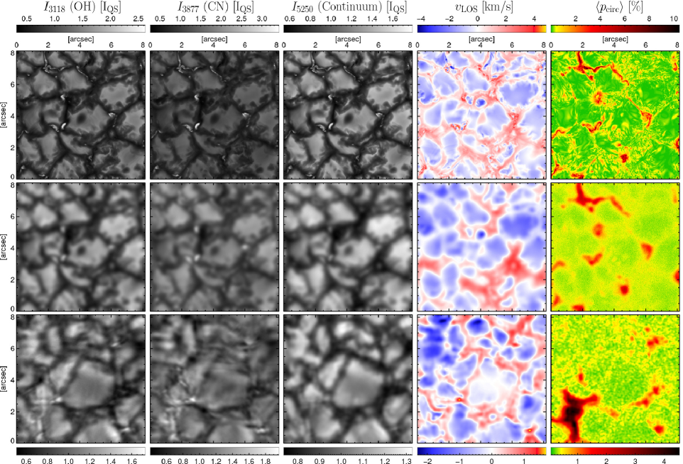
Abbildung 9.2: Intensity maps in the wavelength bands 3118 Å and 3877 Å, as well as for the continuum at 5250.4 Å (three first columns), all normalized to the corresponding mean quiet-Sun intensity level, $I_{\rm{QS}}$. The LOS velocity (positive velocities correspond to downflows) and the circular polarization degree (see main text for definition) are shown in the fourth and fifth columns, respectively. The color bars at the top refer to the undegraded MHD data shown in the first row, while the lower color bars apply to the degraded MHD data (second row) and to the data obtained from the Sunrise observatory (third row).

9.3.1 Simulations versus observations: all pixels

All pixels of all frames contributed to the histograms plotted in Figs. 9.3 to 9.8. In order to ease comparisons between the relatively similarly shaped histograms, the integral over the histograms was always normalized to one.

Fig. 9.3 exhibits histograms of the normalized intensities of the OH data at 3118 Å. The top panel reveals the influence of the various degradation steps on the histogram of the 30 G MHD data. The histogram of the original MHD data is drawn in black. Öriginalmeans that the Stokes $I$ spectra are multiplied with SuFI’s filter transmission profile but no other degradation steps have been applied. The blue line represents spectrally and spatially degraded data, while the red line displays the fully degraded data, i.e. after spectral, spatial, stray light, and noise degradation. A comparison of the black with the blue line shows the influence of the spatial degradation. The noise hardly changes the histograms in Figs. 9.3 to 9.7 and hence the difference between the blue and the red line is mainly due to stray light.

The fully degraded MHD data are then compared with the SuFI observations colored in green. The degradation of the simulated data reduces the rms contrast in the OH band from 32.4 % down to 21.1 % which is 0.9 % higher than the observational contrast of 20.2 %. Though all histograms show a certain amount of asymmetry, the histogram of undegraded simulated data indicates a superposition of two populations: the first one consists of intergranular pixels with low intensities, the second one contains bright pixels from the granules or from bright points. This superposition is still somewhat visible after degradation. The observational histogram does not reveal such a clear superposition of two populations.

The bottom panel of Fig. 9.3 displays OH intensity histograms of fully degraded MHD data for different mean unsigned vertical flux densities. The $I_{\rm{QS}}$ for the intensity normalization in the considered spectral band is determined from the 30 G data (closest to our observations). The rms contrast is highest in the field-free case, 22.7 %, decreasing to 18 % in the 200 G simulation (typical mean flux density of a plage region). This reflects the fact that the convection is inhibited by magnetic fields (Biermann, 1941). Without any magnetic field, there are no BPs and hence the fraction of the area covered by dark intergranular lanes is relatively large. With increasing magnetic flux the number density of BPs increases (see discussion of Fig. 9.12) which reduces the area fraction of the darker regions in the intergranular lanes and the rms contrast is reduced as well, but we think that this effect plays only a minor role. Note that the black line of the bottom panel of Fig. 9.3 has not only more dark pixels than the others but it has also more bright pixels. The superposition of two populations is most pronounced in the field-free data but it is not visible in the 200 G data.

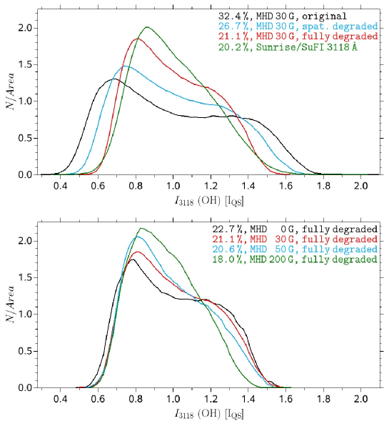
Abbildung 9.3: Intensity histograms of all pixels for the OH band data around 3118 Å. Top panel: The black line corresponds to the original 30 G MHD simulation, the blue line to the spatially degraded data, and the red line to the fully degraded simulation data. The green line displays the Sunrise observations. Bottom panel: Influence of the MHD simulations’ mean flux density on the fully degraded OH intensity histogram. The black line shows a purely hydrodynamical simulation, i.e. without any magnetic field. The mean unsigned vertical flux density was 30 G for the histogram colored in red, 50 G for the blue line, and 200 G for the green line. RMS contrasts are indicated in the text labels.

The intensity histograms of the CN band (3877 Å) are displayed in Fig. 9.4. Compared with the OH histograms, the superposition of two populations is somewhat less pronounced for the simulation data. The rms contrast of the simulated 30 G data is reduced from 30.8 % to 20.5 % after degradation, which is 1.7 % higher than the 18.8 % contrast of the SuFI data. The main difference between the observation and the degraded MHD data is the stronger asymmetry of the synthetic histogram. The rms contrast reduces from 22.8 % to 17.6 % if a 200 G magnetic field is present.

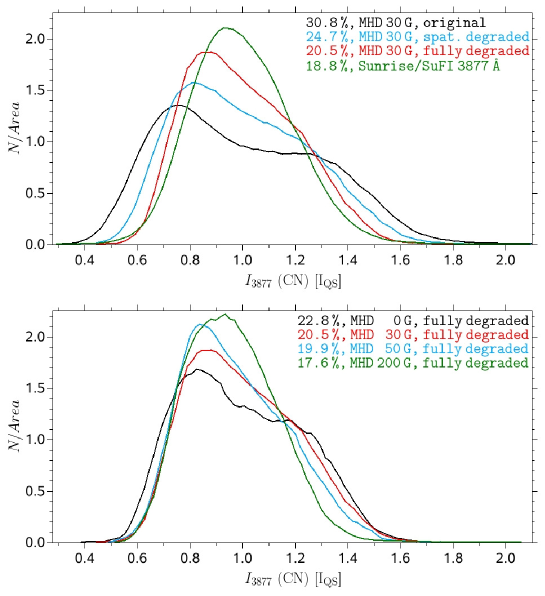
Abbildung 9.4: The same as Fig. 9.3, but for the CN band data around 3877 Å.

Intensity histograms of the IMaX continuum wavelength $5250.2\,\rm{\AA}+192.5\,\rm{m\AA}=5250.4\,\rm{\AA}$ are plotted in Fig. 9.5. In Figs. 9.5 to 9.8, the term öriginalMHD data (black lines in the top panels) implies that the Stokes $I$ spectra are convolved with IMaX’s spectral PSF, but are not otherwise degraded. The full degradation of the 30 G MHD data leads to a decrease in the rms contrast from 22.1 % to 12.1 %, which is exactly the observational contrast. A very good match between the degraded MHD data and the observational data is not only found for the rms contrast (which is not a big surprise; see section 9.2.3), but also for the shape of the histograms. The superposition of two populations can be seen for the undegraded data, but it is not so clear for the degraded simulations. The fully degraded 200 G MHD data have a 2.7 % lower contrast than the corresponding field-free data.

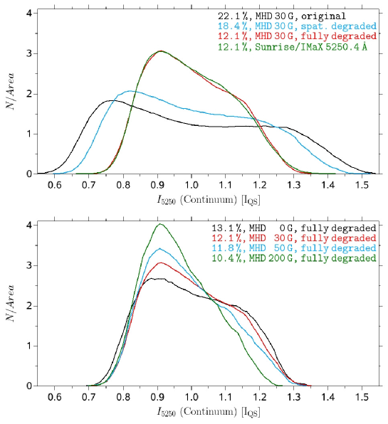
Abbildung 9.5: The same as Fig. 9.3, but for the continuum at 5250.4 Å.

Fig. 9.6 exhibits histograms of the LOS velocity as determined from the Gaussian fit of the twelve scan positions of the Stokes $I$ profiles of the 5250.2 Å line. Since an absolute wavelength calibration of the Sunrise/IMaX data has not been done, we decided to force the observational LOS velocities to have the same mean value as the degraded 30 G MHD data. The standard deviation of the 30 G simulation is reduced by the degradation from 1050 m s^-1 to 580 m s^-1, which is close to the standard deviation of the observed value of 670 m s^-1. The histograms are only weakly asymmetric. Small mean flux densities (0-50 G) led to almost identical velocity histograms. Increasing the average vertical field to 200 G significantly impedes the convection, reducing the standard deviation of the velocities to 460 m s^-1.

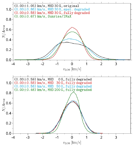
Abbildung 9.6: Same as Fig. 9.3, but for the LOS velocity as retrieved from a Gaussian fit to the Stokes $I$ profile of Fe i 5250.2 Å. Mean values and their standard deviations are indicated in the text labels. Negative velocities are upflows.

Histograms of the 5250.2 Å line widths are displayed in Fig. 9.7. The degradation of the 30 G simulation data (top panel) causes a shift of the position of the histogram’s maximum towards larger line widths coupled with an increase in the width of the histogram, bringing it closer to the histogram of the observed values. Thus the histograms of the degraded simulations and the observations display a reasonable match for the mean values, but a significant mismatch of their widths, i.e. the mean as well as the most common line widths of the simulated profiles are close to the observed values, but the scatter of the line widths is clearly larger for the observational data. The middle panel of Fig. 9.7 shows how the MHD line width histogram depends on the mean flux density. A larger magnetic flux increases the mean value of line widths as well as the standard deviation mainly owing to an increased number of larger line width values (partly due to enhanced Zeeman splitting). The number of small line width values is hardly influenced by the mean flux density and hence none of the considered fluxes matches the observational histogram well.

In the bottom panel of Fig. 9.7 we demonstrate the influence of the secondary peaks of IMaX’s spectral PSF on the degraded 30 G MHD line width histogram. In particular the approximation of the spectral PSF of IMaX by a Gaussian function led to a significantly increased discrepancy between observation and simulation. The best match was reached by doing a full 20-lines synthesis and using the measured spectral PSF for the degradation. Note, that convolving with a 85 mÅ Gaussian, or restricting the line synthesis to just Fe i 5250.2 Å left the histograms of all other quantities considered in this study practically unchanged.

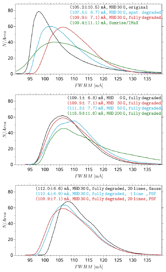
Abbildung 9.7: Top and middle panel: Same as Fig. 9.3, but for the spectral line width (FWHM) as retrieved from a Gaussian fit to the Stokes $I$ profiles of Fe i 5250.2 Å. Bottom panel: Influence of different approximations of the spectral synthesis and degradation on the histograms of the spectral line width of the degraded 30 G MHD data. The spectra were fully degraded in all three plotted cases. The black line corresponds to the histogram obtained when the filter transmission profile was approximated by an 85 mÅ Gaussian instead of the measured spectral PSF. The blue line corresponds to a spectral synthesis of only the 5250.2 Å line, i.e. the 19 neighboring lines were not synthesized. For comparison reasons, the red line of the top panel is plotted again and corresponds to the 20-lines synthesis and spectral degradation with the measured spectral PSF.

Histograms of the circular polarization degree $\langle p_{\rm{circ}}\rangle$ as defined in Eq. (9.1) are given in Fig. 9.8. As for the line widths, we found a strong asymmetry in all histograms. This time the match between the degraded 30 G simulation and the observation was remarkably good. The spatial degradation as well as the stray light contamination made the histogram more narrow and left the maximum position nearly unchanged. The influence of the noise was dominant as can be seen by comparing the magenta line (spectral + spatial + stray light degradation) and the red line (spectral + spatial + stray light + noise degradation). The noise broadens the histogram and shifts the maximum position towards higher polarization values. Note that in contrast to $\langle p_{\rm{circ}}\rangle$ the histograms of all other parameters considered so far were hardly affected by noise.

The middle panel of Fig. 9.8 displays the dependence of the fully degraded MHD histogram on the mean vertical flux density. The maximum position and the width of the histograms increase with mean flux density. The 0 G simulation (which had no magnetic field at all) has no intrinsic polarization, so that the black line is entirely due to noise that was introduced as part of the degradation. This pure noise histogram differs clearly from the observational histogram, so that from such variations of the mean MHD flux we estimated that the Sunrise data correspond to an average LOS field of circa 25 G. (Even the 30 G simulations shown in the top panel of Fig. 9.8 exhibit a slightly too large mean flux density compared to our observation.) We note, however, that all simulations considered here started with an initially homogeneous, vertical and unipolar field. A comparison with simulations with a different initial condition (or a different Reynolds number) could result in a different estimate of the magnetic field in the observed region (see, e.g., Danilovic et al., 2010; Pietarila Graham et al., 2010). Also how exactly the circular polarization degree is normalized (e.g. division by $I_{\rm{i}}$ as in Eq. (9.1), division by $I_{\rm{12}}$ (local continuum), or division by $\langle I_{\rm{12}}\rangle=I_{\rm{QS}}$, i.e. the mean continuum, see Eq. (9.2)) can have a slight influence on the estimated average field strength. Additionally, a possible cross talk from Stokes $Q$ or $U$ into Stokes $V$, which can not be corrected due to the lack of Stokes $Q$ and $U$ signals in the IMaX L12 data, could influence our estimate of the mean MHD flux.

The dependence of the degraded 30 G MHD polarization histogram on the noise level, which was added to all Stokes images, is shown in the bottom panel of Fig. 9.8. Three noise levels between $3.00\times 10^{-3}I_{\rm{QS}}$ and $3.60\times 10^{-3}I_{\rm{QS}}$ (see text labels) are plotted in different colors. Again, the position of the maximum and the width of the histograms increase with noise levels. Nevertheless, noise level and mean MHD flux density can both be fitted to the observational histogram unambiguously since small variations of the mean flux density mainly changes the amplitude and the width of the histogram, while a small variation of the noise level mainly shifts the maximum position. The best-fit noise level was determined to be $\sigma_{\rm{fit}}=3.30\times 10^{-3}I_{\rm{QS}}$, which is somewhat lower than the standard deviation of the observed Stokes $V$ continuum signals, $\sigma_{\rm{all}}=3.77\times 10^{-3}I_{\rm{QS}}$, because the assumption of a signal-free Stokes $V$ continuum is not entirely true. Such a signal was found by Borrero et al. (2010), but was restricted to 0.005 % of all their spatial pixels. Since we do not know how strongly the area covered by these signals increases with decreasing threshold, we use the $\sigma_{\rm{fit}}$ value as an approximation of the true noise level.

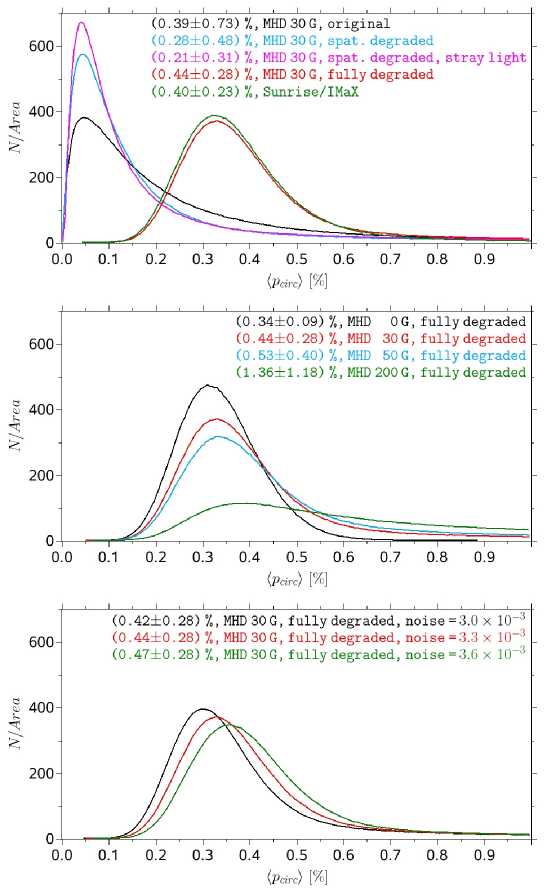
Abbildung 9.8: Histograms of the circular polarization degree $\langle p_{\rm{circ}}\rangle$ as retrieved from the Stokes $I$ and $V$ profiles of Fe i 5250.2 Å (see Eq. (9.1) for definition). Top panel: The black line corresponds to the original 30 G MHD simulation, the blue line to the spatially degraded data, the magenta line represents the histogram after stray light contamination has been added on top. Finally, the red line corresponds to the fully degraded 30 G simulation. The green line displays the Sunrise/IMaX observations. Middle panel: Influence of the MHD simulations’ mean flux density on the fully degraded polarization histogram. The black line shows a purely hydrodynamical simulation, i.e. without any magnetic field. The mean unsigned vertical flux density was 30 G for the histogram colored in red, 50 G for the blue line, and 200 G for the green line. The noise level was always $3.30\times 10^{-3}\leavevmode\nobreak\ I_{\rm{QS}}$. Bottom panel: Influence of the noise level. The flux density was always 30 G. The noise levels in units of the mean quiet-Sun intensity are printed as text labels.

9.3.2 Simulations versus observations: bright points

We now compare BP properties between Sunrise observations and the degraded 30 G simulations. From the flux tube paradigm one would expect kilo-Gauss fields for the BPs and hence strong polarization signals, but Riethmüller et al. (2010, see their Fig. 2, panel h) find that the majority of the BPs is only weakly polarized. We use the BP detection method applied by Riethmüller et al. (2010) for a direct comparison with their results.

First of all, we need an additional step in the pre-processing of the observational data because IMaX and SuFI differed significantly in their plate scales and also we had a slight difference in the plate scales of the various SuFI wavelengths. Therefore we re-sampled all data to the common plate scale of 0$\mbox{.}^{\prime\prime}$0207 Pixel^-1 (original plate scale of the SuFI 2995 Å images) via bilinear interpolation. With the help of cross correlation functions the two instruments’ common field of view (FOV) was identified. Finally, the larger IMaX FOV was cropped to the smaller 13^′′$\times$37^′′ SuFI FOV.

We then manually identified the BPs’ peak intensity in the CN images because of their good visibility in that molecular band (Schüssler et al., 2003). The local intensity maximum in an 11$\times$11 pixel (i.e., 0$\mbox{.}^{\prime\prime}$22$\times$0$\mbox{.}^{\prime\prime}$22) patch surrounding each BP detected at 3877 Å was determined for each of the other wavelengths. This method takes into account that the various wavelengths are formed in different atmospheric layers so that inclined features may appear at slightly different horizontal positions at different wavelengths. Also, the dark background (DB) close to the BPs was retrieved. It was defined as the darkest pixel within 0$\mbox{.}^{\prime\prime}$3 of each BP. We extended the simple and manual BP detection method of Riethmüller et al. (2010) by the determination of the BP boundaries with the help of a multilevel tracking (MLT) algorithm (see Bovelet & Wiehr, 2001). The MLT algorithm determined the intensity range of the CN images and subdivided this into 25 equidistant levels. Starting with the highest intensity level all pixels were found whose intensity exceeds this level. This led to several contiguous two-dimensional structures, which were tagged with a unique number. The obtained structures were extended pixel by pixel as long as the intensity was greater than the next lower level. Then the algorithm searched through the whole image again to find all pixels whose intensity was greater than the next lower level, which often led to newly detected contiguous structures. This procedure was repeated until the minimal intensity level was reached. At the end, every pixel belonged to exactly one contiguous structure. Finally, all pixels that had an intensity lower than 50 % of the local min-max range were rejected, which led to the boundary of the BPs. A more detailed description of MLT, including some illustrative figures, was given by Riethmüller et al. (2008d) where the algorithm was applied to the detection of umbral dots. The BP boundary detection via MLT was applied to the SuFI intensity images, to the IMaX continuum intensity images, and also to the maps of the $\langle p_{\rm{circ}}\rangle$ (see section 9.2.3). We identified 121 BPs in the nine observational data sets. This number is limited by few L12 IMaX data sets available. The corresponding BP number density was 0.05 BPs per $\rm{Mm}^{2}$, which is 1.7 times higher than the value found by Jafarzadeh et al. (2013) in the Ca ii H channel of Sunrise/SuFI. The difference likely stems from the restriction to small BPs by Jafarzadeh et al. (2013).

We applied the same manual detection method to the degraded CN images of the 30 simulation data sets with 30 G field strength. Here we found 277 BPs (0.26 BPs per $\rm{Mm}^{2}$). We also detected BPs in the 30 undegraded CN images. Owing to the much higher spatial resolution of the undegraded data, we found a lot more BPs there, in total 898 (0.83 BPs per $\rm{Mm}^{2}$), although many of them were relatively small. (Histograms for the BP diameter are given below, see Fig. 9.21.) In case of the synthetic data, the boundaries of our manually detected BPs were obtained by applying the MLT algorithm to the CN, OH, and 5250.4 Å intensity images, to the maps of the circular polarization degree, and since we also discuss BP properties which were a direct output of the MHD calculations such as the magnetic field strength, we additionally applied the MLT algorithm to the field strength maps at constant optical depth $\log(\tau)=0$ and $\log(\tau)=-2$. The determination of various boundaries for the same set of BPs takes into account that the magnetic features change in size with height and do not always overlap one to one with their brightness enhancements.

Histograms of various quantities in BPs are displayed as red lines in Figs. 9.9 to 9.12. For comparison, the blue lines represent histograms of the same parameters in the dark background (DB, defined as the darkest pixel within 0$\mbox{.}^{\prime\prime}$3 of each BP’s peak position). Likewise for comparison, we plot in green the corresponding histograms over all pixels in the images. These histograms have already been plotted in Figs. 9.3, 9.5, 9.6, and 9.8. The histograms of Figs. 9.9 to 9.12 are normalized to their maximum which turns out to be more favorable for comparison between histograms of significantly different shapes than normalization by their integrals. Figures 9.9 to 9.12 compare the set of 121 BPs detected from the Sunrise observations (upper panels) with the set of 277 BPs detected from the degraded 30 G MHD simulations (bottom panels). Additionally, the bottom panels in Figs. 9.9 to 9.11 show the histogram of the 898 BPs which we detected in the undegraded MHD data (black lines), so that the influence of the degradation is visible.

Histograms of the BPs’ peak intensity (intensity of the brightest pixel of a BP) in the OH band at 3118 Å are drawn in Fig. 9.9. As expected, the highest BP intensities coincide with the highest intensities found in these images. The observed BPs exhibit a peak intensity range of $(0.86-1.97)\leavevmode\nobreak\ I_{\rm{QS}}$ (with a mean value of $1.37\leavevmode\nobreak\ I_{\rm{QS}}$), which is considerably higher than the range of $(0.73-1.58)\leavevmode\nobreak\ I_{\rm{QS}}$ with a mean value of $1.05\leavevmode\nobreak\ I_{\rm{QS}}$ obtained from the degraded simulations. Hence the observed BPs are brighter. The observed DB histogram is also broader than the simulated one.

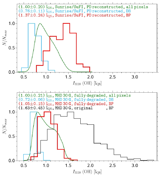
Abbildung 9.9: Histograms of the bright point (BP) peak intensity in the 3118 Å OH band (red lines), the intensity histograms of the BPs’ dark background (blue lines), and the histograms of all pixels (green lines). Mean values and standard deviations are given in the text labels. The top panel shows the histograms obtained from the observational data recorded by the SuFI instrument, the bottom panel displays the same for the degraded 30 G MHD simulations. The BP histogram of the undegraded MHD data is indicated in the bottom panel by the black line.

Fig. 9.10 shows histograms of the BPs’ peak intensity in the continuum at 5250.4 Å. Again, the range covered by the observational BP histogram, $(0.82-1.24)\leavevmode\nobreak\ I_{\rm{QS}}$, is larger than that covered by the simulational BP histogram, $(0.80-1.18)\leavevmode\nobreak\ I_{\rm{QS}}$, although the discrepancy is not so marked. In addition, we found an almost perfect agreement between observation and simulation for the histograms of all pixels and a rather good match for the DB histograms. Also in contrast to the OH band, the highest intensities in the 5250.4 Å continuum images do not belong to BPs but to the brightest parts of granules.

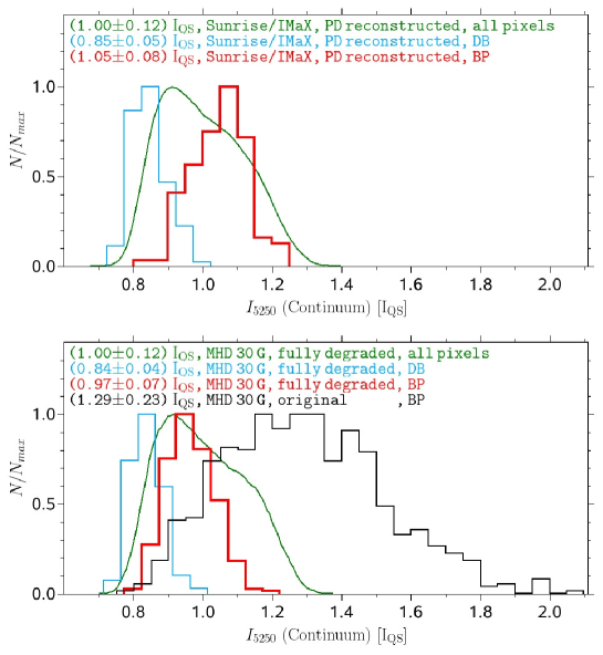
Abbildung 9.10: Same as Fig. 9.9, but for the peak intensity at the 5250.4 Å continuum.

As mentioned above, the LOS velocity was retrieved from a Gaussian fit to Fe i 5250.2 Å Stokes $I$. The LOS velocities of all pixels belonging to a particular BP in the 5250.4 Å continuum are averaged and this averaged velocity is then assigned to that BP. The red lines of Fig. 9.11 exhibit histograms of such spatially averaged BP velocities. The standard deviations of the observational histograms agree with the degraded simulations, but the observed BPs and their DB display larger downflows. Clearly, the BPs’ LOS velocity lies on the downflow side of the distribution for the whole map. The velocities of the observational BPs range between $-980$ m s^-1 and 1510 m s^-1, with an average downflow of 600 m s^-1. The downflow of the DB is on average 300 m s^-1 stronger. The BPs of the simulations show LOS velocities ranging from $-1180$ m s^-1 to 1620 m s^-1 with a mean downflow of 270 m s^-1. Here, the downflow of the mean DB is only 170 m s^-1 stronger than for the BPs. The original, undegraded simulations exhibit much larger downflows.

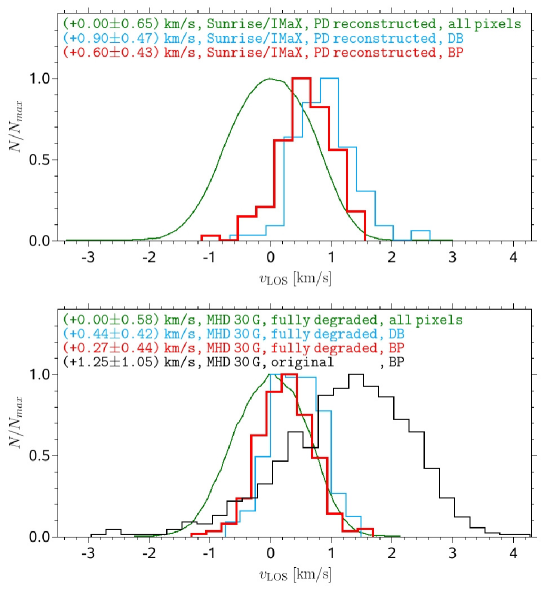
Abbildung 9.11: Same as Fig. 9.9, but for the LOS velocity.

Histograms of the BPs’ circular polarization degree (peak polarization within the BP boundary as determined from the polarization maps) can be seen in Fig. 9.12. Firstly, a comparison of the upper panel of Fig. 9.12 (IMaX observations with 12 scan positions) with Fig. 2, panel (h) of Riethmüller et al. (2010) (IMaX observations with 5 scan positions) shows that even for a significantly improved wavelength sampling, we find that most BPs are only weakly polarized. The strongest BP polarization degrees observed in the V5-6 mode reached 9.1 %, while they reached only 6.8 % in the L12-2 mode. This difference is caused by the fact that we averaged over all twelve scan steps in the L12-2 mode and hence over more scan positions close to the continuum (i.e. low polarization signals) than in the V5-6 mode. By interpolating Stokes $V$ to the wavelength positions of the V5-6 mode we obtained similar polarization degrees as found in the V5-6 data by Riethmüller et al. (2010). Also, the noise levels of the two data sets were comparable. We also calculated the histogram of the circular polarization degree of the set of V5-6 BPs analyzed by Riethmüller et al. (2010) (not shown) and compared it with their histogram of the total polarization degree shown in Fig. 2, panel (h) of Riethmüller et al. (2010). From the similarity of the two histograms we concluded that the Stokes $Q$ and $U$ signals are negligible for a statistical BP study.

A comparison of the observed and degraded 30 G simulation BP $\langle p_{\rm{circ}}\rangle$ histograms revealed a good agreement for most of the BPs, but a population of BPs showing strong $\langle p_{\rm{circ}}\rangle$ is found only in the observations. We can rule out a possible over-reconstruction of the IMaX data as the cause of these large $\langle p_{\rm{circ}}\rangle$ because the rms contrasts matched rather well. Since we also applied the BP boundary detection via MLT to the circular polarization maps, we were able to determine the effective diameter of the polarized features, defined as the diameter of a circle of area equal to that within the $\langle p_{\rm{circ}}\rangle$ boundary of the BP. We found that 6 of the 121 observed BPs had $\langle p_{\rm{circ}}\rangle>4.8\,\%$ (strongest BP polarization of the 30 G simulation) and their diameter was on average 399 km, while the other 115 BPs had a mean diameter of only 299 km. The long tail towards stronger polarization degrees, which we found in the observational BP histogram, is caused by large and strongly polarized BPs which were not present in the 30 G simulations. For comparison reasons, we also plotted the histogram of $\langle p_{\rm{circ}}\rangle$ of the 285 BPs that we detected in the 10 degraded snapshots of our 200 G simulations (magenta line of the bottom panel of Fig. 9.12). There the mean polarization degree was 3.32 %, the strongest value being 6.4 %. The number density was 0.79 BPs per $\rm{Mm}^{2}$.

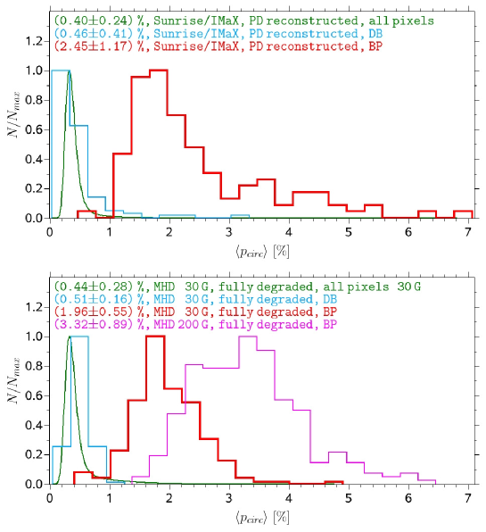
Abbildung 9.12: Same as Fig. 9.9 for the spatial peak value of the circular polarization degree. Additionally, the magenta line shows the histogram of the BP polarization for the degraded 200 G MHD simulations.

9.3.3 Why is the majority of bright points weakly polarized?

The bottom panel of Fig. 9.12 exhibits many synthetic BPs which are only weakly polarized. The same was noted by Riethmüller et al. (2010). This weak polarization could be due to the fact that most BPs have intrinsically weak fields, contrary to the standard flux tube theory (Spruit, 1976), or they are very highly inclined, nearly horizontal, also contrary to theory for strong fields (Schüssler, 1986). Alternatively, they could be spatially unresolved at the spatial resolution reached by Sunrise, or the weak Stokes $V$ could also be caused by thermal weakening of Fe i 5250.2 Å in BPs. We searched for the cause by analyzing the simulation data.

BPs are often modeled by nearly vertical slender flux tubes. In the flux tube model, only magnetic field strengths in the kilo-Gauss range can explain the brightnesses that are observed in BPs. The field increases the magnetic pressure which leads to an evacuation inside the tube and hence a depressed optical depth unity surface. The lateral inflow of heat through the walls of the flux tube makes it hot and bright.

To determine what polarization signals can be expected for kilo-Gauss fields, we synthesized Stokes profiles for a standard atmosphere, the HSRASP (Chapman, 1979), assigned a zero velocity and a height independent field strength of 1 kG. The synthetic profiles were then convolved with the spectral PSF of IMaX and the Stokes $V$ values at the twelve scan positions of the IMaX L12-2 mode were used to calculate $\langle p_{\rm{circ}}\rangle$ according to Eq. (9.1). A value of 10.71 % was obtained. This value is significantly higher than the mean value of $\langle p_{\rm{circ}}\rangle$ of 1.96 % obtained from the fully degraded data.

To analyze the influence of the several degradation steps on the mean BP polarization, we used the set of 898 BPs that we detected in the undegraded CN images for the original MHD data and determined their peak $\langle p_{\rm{circ}}\rangle$ values (see black line in Fig. 9.13), for the data that were spectrally and spatially degraded (blue line), for the additionally stray light contaminated images (magenta line), and the fully degraded data (red line of Fig. 9.13). The spatial degradation reduced the mean BP polarization from 6.66 % down to 2.37 %. The stray light led to a further reduction down to 1.45 % and the noise increased the mean value to 1.74 %. In contrast to the histograms of all pixels (top panel of Fig. 9.8), here the noise was not the main contributor but the spatial degradation, because the BP $\langle p_{\rm{circ}}\rangle$ values were much higher than the noise level.

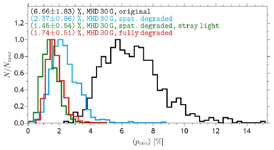
Abbildung 9.13: Influence of the various degradation steps on the histogram of the BP circular polarization degree. The degradation was applied to the 30 G MHD simulations. The black line corresponds to the data that were only spectrally degraded. An additional spatial degradation is shown in blue. The green line contains also the stray light contamination and the fully degraded BPs are colored in red, i.e. including noise.

Note that the red line in the bottom panel of Fig. 9.12 and the red line of Fig. 9.13 are not identical. Both histograms were retrieved from the same fully degraded $\langle p_{\rm{circ}}\rangle$ maps, but the lower panel of Fig. 9.12 was calculated for the 277 BPs that were detected in the degraded CN images while Fig. 9.13 displays the 898 BPs detected from the undegraded CN images, which contained many small BPs and hence led to a smaller mean value of 1.74 % compared to 1.96 % for the 277 BPs detected in the degraded CN images.

Even at original resolution of the simulations the average $\langle p_{\rm{circ}}\rangle$ is only 6.66 % and only 2.6 % of all BPs reach the 10.71 % retrieved from the 1 kG HSRASP atmosphere. This remaining discrepancy can be explained by the high temperature sensitivity of the Fe i line at 5250.2 Å, as illustrated in Fig. 9.14, where two pixels taken from the simulation data are compared. The pixel colored in blue belongs to a faint BP with a low brightness in the CN band, but one that is still identified as a BP, while the pixel colored in red is part of a BP with a high contrast. Panel (a) of Fig. 9.14 shows the vertical temperature stratification where the atmospheric height is given in logarithmic units of $\tau$, which is the optical depth of the continuum at the wavelength of 5000 Å. In the middle photosphere (where the spectral line is mainly formed), the red pixel’s temperature is about 800 K higher than the temperature of the blue pixel, but in the lower and upper photosphere both temperatures are almost the same. The vertical stratification of the magnetic field strength is displayed in panel (b). In the middle photosphere, e.g. at $\log(\tau)=-2$, the blue pixel reveals a field strength of roughly 650 G, while the red pixel has a field strength of 1200 G. As typical for the flux tube model of BPs, at $\log(\tau)=0$ both pixels show a magnetic field stronger than 1 kG that is nearly vertically oriented (the mean field inclinations of the two pixels are $8.9^{\circ}$ and $7.6^{\circ}$). The original Stokes $I/I_{\rm{QS}}$ signals of the twelve scan positions of the 5250.2 Å line are shown in panel (c). The intensity of the red pixel is higher than $I_{\rm{QS}}$ while it is lower in the blue pixel. The most striking feature of the figure is the minimal line depth of the 5250.2 Å line in the red pixel. This is partly due to the large Zeeman splitting caused by the large field strength in this pixel. The strong temperature sensitivity also contributes just as much. The temperature sensitivity originates not just in the increased ionization of iron as the temperature is raised, but also from the excitation potential of the lower level of this line of only 0.12 eV. This weakening is also conspicuous in the Stokes $V/I_{\rm{QS}}$ profiles of panel (d). Although the red pixel has a higher magnetic field strength, its circular polarization degree of 1.8 % is much smaller than that of the blue pixel, 6.8 %. The ratio 1.8 %/6.8 % is larger than the ratio of the line depths, due to the contribution of the magnetic field which is stronger for the red pixel (obviously Zeeman saturation, Stenflo, 1973, is not complete, so that a residual Zeeman sensitivity is present).

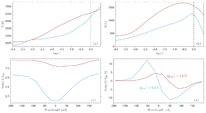
Abbildung 9.14: Demonstration of a weak polarization signal owing to the strong temperature sensitivity of the Fe i line at 5250.2 Å by a comparison of a pixel in a particularly bright BP (red lines) with a pixel located in a much less bright BP (blue lines). Panel (a) exhibits the vertical temperature stratification as a function of $\log(\tau)$ at 5000 Å, panel (b) the magnetic field strength stratification. Panels (c) and (d) depict the Stokes $I/I_{\rm{QS}}$ and $V/I_{\rm{QS}}$ signals from the original MHD data at the twelve IMaX L12-2 scan positions in the line.

The temperature effect is statistically relevant for the BPs in general. To show this, in Fig. 9.15 we plot the circular polarization degree versus the magnetic field strength at $\log(\tau)=-2$ (peak values for both quantities) for all 898 BPs in the original 30 G MHD data. At $\log(\tau)=-2$ these BPs have a mean temperature of 5102 K, and all BPs hotter than the mean temperature are colored in red, the cooler ones in blue. The solid lines are the linear regressions of the two BP classes. We recognize a clear trend that for a given field strength, the BPs having a higher temperature show a weaker $\langle p_{\rm{circ}}\rangle$ than cooler BPs, although the scatter is large.

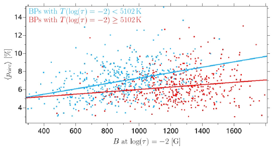
Abbildung 9.15: Circular polarization degree versus magnetic field strength at $\log(\tau)=-2$ as retrieved for the 898 BPs from the original 30 G MHD data. Pixels with $T\geq 5102$ K are colored in red, cooler pixels in blue. The solid lines are linear regressions.

Since the Stokes $V$ normalization to $I_{i}$, chosen by Riethmüller et al. (2010), could enhance the effect of the line weakening of $\langle p_{\rm{circ}}\rangle$ we also considered other formulas to analyze the BP polarization or field strength, respectively:

$$\langle p_{\rm{circ}}^{\rm{QS}}\rangle=\frac{1}{12I_{\rm{QS}}}\sum_{i=1}^{12}{\left|V_{i}\right|}\leavevmode\nobreak\ ,$$ (9.2)

$$\langle B_{\rm{LOS}}\rangle=\frac{1}{N}\sum_{i=1}^{N}{\frac{4\pi cm_{e}}{e\lambda_{0}^{2}g}\left|\frac{V_{i}}{(\rm{d}I/\rm{d}\lambda)_{i}}\right|}\leavevmode\nobreak\ .$$ (9.3)

The scatterplot for $\langle p_{\rm{circ}}^{\rm{QS}}\rangle$ (not shown) exhibits the same qualitative behavior than that for $\langle p_{\rm{circ}}\rangle$ (shown in Fig. 9.15), so that the temperature effect cannot be reduced by this widely used normalization for the circular polarization calculation.

Eq. (9.3) is based on the weak field approximation which holds if the Zeeman splitting is much smaller than the line width (Landi Degl’Innocenti & Landolfi, 2004). The derivative of Stokes $I$ was determined from the Gaussian fit of the Stokes $I$ profile. $c$, $m_{e}$, and $e$ have the usual meaning, $\lambda_{0}=5250.2$ Å is the reference wavelength, and $g=3$ is the effective Landé factor of the line. To avoid division by zero, the sum in Eq. (9.3) had only been calculated over the $N$ scan positions with $\left|\rm{d}I/\rm{d}\lambda\right|>3\sigma$, where $\sigma$ is the ratio of the Stokes $I$ noise level and the scanning step size. A scatterplot of $\langle B_{\rm{LOS}}\rangle$ versus the magnetic field strength at $\log(\tau)=-2$ (not shown) revealed that Eq. (9.3) very significantly reduces the effect of the line weakening. The $\langle B_{\rm{LOS}}\rangle$ values obtained from applying Eq. (9.3) on observational and degraded synthetic data are plotted in Fig. 9.16. Similar to $\langle p_{\rm{circ}}\rangle$ (Fig. 9.12), $\langle B_{\rm{LOS}}\rangle$ shows a long tail of stronger fields which is more pronounced for the observational data. Only 9.9 % of the observed BPs and 3.6 % of the synthetic BPs yielded $\langle B_{\rm{LOS}}\rangle$ values higher than 1 kG.

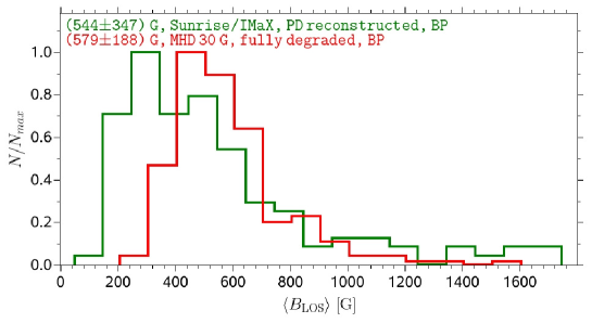
Abbildung 9.16: Histograms of the peak value of the BP field strength calculated via the weak field approximation (see main text). The green line shows the observed BPs, the red line displays the BPs from the degraded 30 G MHD data.

9.3.4 Properties of simulated bright points

In sections 9.3.2 & 9.3.3 we showed that the MURaM MHD simulations reproduce the properties of the observed BPs reasonable well. Therefore we can obtain a better understanding of the physical phenomena underlying BPs by analyzing BP properties in undegraded simulations. This we now proceed to do. In the following we used the 898 BPs detected in the undegraded CN images. It is this set of BPs that underlies Figs. 9.17 to 9.20 and Fig. 9.22.

Fig. 9.17 shows histograms of the BP peak magnetic field strength taken directly from the 30 G MHD simulations. The peak values were determined as the maximum field strength at a given optical depth within a BP. Owing to lateral force balance, the decreasing gas pressure with height and the need for magnetic flux conservation, the flux tubes expand, so that the BP field strength drops from an average of 1755 G to 1072 G at $\log(\tau)=-2$. At optical depth unity, only 14 of the considered 898 BPs had a field strength lower than 1000 G, i.e. 98 % of the BPs were in the kilo-Gauss range, the strongest BP field strength was found to be 2825 G, the weakest one was 721 G. On average, the DB field strength is an order of magnitude lower than in the BPs.

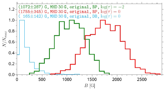
Abbildung 9.17: Histograms of the magnetic field strength of the BPs in the middle photosphere (green line) and of the BPs (red line) and the DB (blue line) in the lower photosphere as retrieved from the undegraded 30 G MHD data. Mean values and their standard deviations are given in the text labels.

Fig. 9.18 displays the field inclinations (angle between the field vector and the surface normal) of the 30 G MHD BPs at optical depth unity. The inclinations were averaged over all pixels covered by a BP at optical depth unity. The mean inclination of the BPs is $17^{\circ}$, i.e. the BPs are almost vertical as expected from buoyancy considerations (Schüssler, 1986). 4 of the 898 BPs showed inclinations greater than $90^{\circ}$, i.e. their magnetic field direction had been reversed from the initial condition of a homogeneous unipolar field. The field in the DB, in contrast, displays all possible inclination values, where vertical fields of either polarity are slightly preferred. The distribution of the field inclinations of all pixels is quite similar to the distribution of an isotropic field.

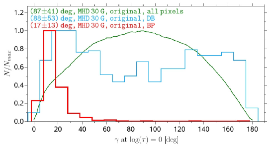
Abbildung 9.18: Histograms of the magnetic field inclination at optical depth unity of BPs, DB, and of all pixels. The color coding is the same as in Fig. 9.9.

In Fig. 9.19 we compared the BP temperatures between the middle photosphere and the lower photosphere. The temperatures were averaged over all pixels of a BP as determined by the MLT algorithm applied to the CN maps. The mean BP temperature in the middle photosphere was 442 K higher than the mean quiet-Sun temperature. The mean DB temperature was 31 K lower than the mean quiet-Sun value. In the lower photosphere, the mean BP temperature was 191 K higher than the mean quiet-Sun temperature, while the dark background was 416 K colder than the quiet Sun. The temperature gradient in the BP and in the DB was significantly lower than on average.

Abbildung 9.19: Histograms of the temperature for the simulated BPs (red lines), for the BPs’ dark background (blue lines), and for all pixels in all frames (green lines). Mean values and their standard deviations are given in the text labels. The top panel shows the temperature at $\log(\tau)=-2$, the bottom panel at optical depth unity (note the different $T$ scales).

Fig. 9.20 displays histograms of the LOS velocity obtained directly from the MHD calculations. The LOS velocities were averaged over all pixels of a BP as determined by the MLT algorithm applied to the 5250.4 Å continuum intensity images. At an optical depth of $\log(\tau)=-2$ (top panel) the mean BP velocity was a moderate downflow of 1.06 km s^-1. With it the BPs revealed a stronger downflow than the DB with on average 0.16 km s^-1. In the lower photosphere at $\log(\tau)=0$ (bottom panel), the LOS velocities of the BPs showed a strong downflow of 3.17 km s^-1. This time the DB downflow was on average slightly stronger with 3.35 km s^-1. The histogram of all pixels (green line) clearly shows a superposition of two populations. The pixels from the interior of the granules formed the first population with an upflow of around $-2$ km s^-1 as the most numerous velocity. The second population corresponds to intergranular lanes with a 3 km s^-1 downflow as the most numerous velocity.

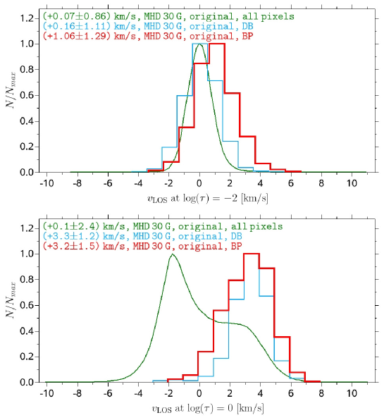
Abbildung 9.20: Same as Fig. 9.19 for the LOS velocities (vertical component of the velocity vector taken directly from the MHD output).

Fig. 9.21 compares histograms of the effective BP diameter between the Sunrise observations and various 30 G MHD simulations. The diameters were calculated from the BP boundaries as determined from the CN intensity images. The observed mean BP diameter of 334 km (red line) was fairly similar to the mean diameter of the degraded synthetic BPs, 330 km (black line). The influence of the degradation can be seen by comparing this black line with the blue line, showing the histogram of the undegraded MHD simulations. The degradation increased the mean BP diameter from 129 km to 330 km. The cell size of the MHD grid may also influence the BP diameters. We repeated the 30 G MHD simulation, the full spectral line synthesis of the CN band, and the BP detection for a cell size of 20.8 km while all other parameters were unmodified. 475 BPs were found in the 30 snapshots of $6\times 6\,\mathrm{Mm}^{2}$ size (number density was 0.44 BPs per $\rm{Mm}^{2}$) with a mean BP diameter of 163 km (green line). This dependence of BP diameter and number density on the grid size of the simulations is interesting in the sense that it indicates that an even smaller grid size could result in smaller BPs, which casts doubts on the claims of Crockett et al. (2010) that they resolved essentially all BPs, from the comparison of BP area distributions from observations and from simulations. However, the employed simulations had a grid size of 25 km, so that true BP sizes are almost certainly smaller than was claimed. Note that the green line of Fig. 9.21 is the only one result in this study that corresponds to an MHD cell size of 20.8 km, all other MHD results stem from 10.4 km simulations.

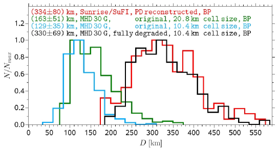
Abbildung 9.21: Histograms of the effective BP diameter for the observed BPs (red line), for the undegraded MHD BPs simulated with a cell size of 20.8 km (green line), for the undegraded MHD BPs simulated with a cell size of 10.4 km (blue line), and for the degraded MHD BPs simulated with a cell size of 10.4 km (black line).

Finally, we were interested in correlations between certain BP properties by looking at scatterplots. The field strength at optical depth unity, the CN intensity, as well as the 5250.4 Å continuum intensity were only weakly correlated with the BP diameter. The scatterplots (not shown) exhibited a slight increase of the three quantities for large BP diameters. A decrease in the intensities for very large diameters, that we expect for micropores and pores, could not be found by our study owing to the BP detection method, which looked for bright features and not for strongly magnetized ones. Also, the scatterplot of the CN intensity versus the magnetic field inclination at optical depth unity (not shown) revealed nearly no correlation. We found a slight increase in intensity only for the most common inclinations around $17^{\circ}$. A strong correlation was found between the CN intensity and the field strength at optical depth unity, see Fig. 9.22. The binning graph is monotonic over the whole field strength range. Again, a decrease of the intensity for very strong fields could not be found owing to the BP detection method which excluded micropores.

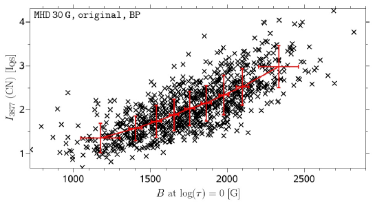
Abbildung 9.22: Scatterplot of the BP peak intensity at 3877 Å versus the magnetic field strength at optical depth unity (black crosses). The BPs were detected from the original 30 G MHD data with a cell size of 10.4 km. The solid red line connects binned values.

9.4 Discussion

The aim of this study is to learn more about magnetic BPs in the solar atmosphere. To achieve this we combine high-resolution observations with realistic radiation-MHD simulations. First we compare a row of parameters deduced from the observations (intensity, LOS velocity, line width, circular polarization degree) with their counterparts obtained from the simulations under conditions matching those of the observations as closely as possible (noise, spatial and spectral resolution and sampling, straylight, etc.). After establishing that the simulations give a reasonable description of the data, both in general and for the BPs in particular, we have employed the simulations to deduce more about the BPs than can be gleaned from the observational data alone.

We observed quiet-Sun regions at disk center with the balloon-borne observatory Sunrise. Photometric data at 3118 Å and 3877 Å as well as spectropolarimetric data at twelve wavelengths in and around the Fe i line at 5250.2 Å were acquired quasi simultaneously. Compared to high-resolution observations with other telescopes, we benefited from the following advantages of Sunrise: a) The Sun was not only observed in the visible but also in the near UV. b) The PSF was measured during the observations, so that the influence of the central obscuration by the secondary mirror, the spiders, and the low-order aberrations like defocus, coma, astigmatism were known and we did not have to rely on a theoretical PSF. c) A stray light analysis was possible owing to observations of the solar limb. d) The data were practically free of seeing effects. By means of that, it was possible to carefully determine the degradations that were acting during the observations and to apply them to the MHD simulations. In contrast to other studies, which worked with opacity distribution functions (ODFs, e.g. Danilovic et al., 2008; Afram et al., 2011), we applied full spectral line syntheses, for the first time also for the OH band at 3118 Å. Our study concentrated on a comparison of the following BP properties at disk center: intensity in the visible and near UV, LOS velocity, and polarization degree, while other studies focussed on center to limb variations of only intensity histograms (Wedemeyer-Böhm & Rouppe van der Voort, 2009; Afram et al., 2011).

A reasonable match between the observations and the degraded simulations was found for the intensity histograms of all pixels for all three considered wavelength ranges as well as for the LOS velocities and the circular polarizations. The intensity histograms of the undegraded 30 G simulations showed a superposition of two populations which was greatly weakened by the degradation and which was not found in the observations. The two populations were also clearly present in comparable simulations with the Stagger and CO⁵BOLD code (Wedemeyer-Böhm & Rouppe van der Voort, 2009; Beeck et al., 2012). Afram et al. (2010) used also the MURaM code and found the same superposition for their undegraded 0 G and 50 G simulations but not for their 200 G data. We can confirm this result by our intensity histograms of the degraded MHD data for varying mean flux densities.

The degradation of our MHD data reduced the rms contrast at 3118 Å from 32.4 % to 21.1 %, at 3877 Å from 30.8 % to 20.5 % and at 5250.4 Å from 22.1 % to 12.1 %. With the help of ODFs, Hirzberger et al. (2010) calculated an rms contrast of 28.3 % at 3118 Å and of 23.9 % at 3877 Å. In both cases, complete spectral line syntheses led to significantly higher contrasts than with the ODF method, although the smaller grid size of the simulation employed by us may also have contributed. For the CN band at 3877 Å, Hirzberger et al. (2010) applied also a full spectral line synthesis but they used an older version of SPINOR whose number of wavelength points was limited. They converted from geometrical heights into optical depths by a different opacity package and they also used a different horizontal grid resolution of 20.8 km. They report an rms contrast of 25.3 % for the undegraded CN data while we found a value of 30.8 % with the improved SPINOR code. The deviation of the rms contrasts between degraded simulations and observations was 0.9 % at 3118 Å, it was negligible at 5250.4 Å, at 3877 Å it was somewhat higher, but at 1.7 % the agreement was still remarkably good, given the various sources of uncertainty, e.g. slightly varying image quality owing to the remaining pointing jitter of the gondola, incomplete spectral line lists, inaccurate atomic or molecular data or neglected non-LTE effects. Given that the computed CN lines are distinctly too strong even for the average quiet Sun (see Fig. 9.1), we expect these last points to play a significant role in producing the discrepancy. Even a comparison between several MHD codes by Beeck et al. (2012) led to a variation in the bolometric intensity contrast of up to 1 %. Hirzberger et al. (2010) found rms contrasts of 18.3 % and 20.1 % for two different Sunrise observations at 3877 Å, while our observation showed 18.8 %. Depending on the ratio of the jitter frequency to the exposure time, different image qualities are possible for observations at different wavelengths. The exposure time of the 3877 Å images was by far the shortest one compared to the other wavelengths.

We found that the various degradation steps considerably influenced the shape of the histograms of various parameters. In particular, we want to emphasize the stray light since it influenced all types of histograms and often it provided the most important contribution to the degradation. This was also found by Wedemeyer-Böhm & Rouppe van der Voort (2009). Additionally, for the line width histogram a good knowledge of the spectral PSF of the instruments is needed. The circular polarization histograms depended strongly on the noise level of the Stokes $V$ images, while the noise level of the Stokes $I$ images as well as the other degradation steps played only a minor role.

Stray light may also contribute to the last remaining discrepancy between the data and the simulations, the larger scatter of the observed 5250.2 Å line widths than in the simulations. We used the continuum images of the IMaX limb observations, but the IMaX stray light may have been somewhat dependent on the wavelength within the spectral line. Due to the sensitivity of the histogram shapes to stray light, we believe that such a wavelength dependence could be a good candidate to explain the larger scatter in the observed line widths. Another possibility is the influence of the evolution of the granulation during the relatively long acquisition time of IMaX of almost 32 s which may also change the line width histogram.

The good match between observation and simulation (only a moderate deviation remained for the scatter of line widths) enhanced our trust in the simulations, so that we used them to probe BP properties. We found a BP number density of 0.05 BPs per $\rm{Mm}^{2}$ in our observations which is at the lower end of the wide spread of values found in the literature: Muller & Roudier (1984) reported 0.04 BPs per $\rm{Mm}^{2}$, 0.12 BPs per $\rm{Mm}^{2}$ were found by Bovelet & Wiehr (2008), 0.3 BPs per $\rm{Mm}^{2}$ by Sánchez Almeida et al. (2004) – all these were quiet-Sun studies, and Berger et al. (1995) analyzed active-region data and resulted in 0.37 BPs per $\rm{Mm}^{2}$. Our BP number density is larger than the 0.03 BPs per $\rm{Mm}^{2}$ obtained by Jafarzadeh et al. (2013) from Ca ii H observations made by Sunrise, but this is likely due to the fact that they restricted their study to features narrower than 0$\mbox{.}^{\prime\prime}$3. On the other hand, the effective BP Diameter was on average 334 km in our observations while most other studies reported somewhat smaller BP diameters, e.g.: Berger et al. (1995) found a mean FWHM intensity diameter of 250 km by taking the smallest dimension across the BP features. Sánchez Almeida et al. (2004) fitted the minor and major axes of the BPs with average values of 135 km and 230 km, respectively. Utz et al. (2009) reported a decrease in the mean BP diameter from 218 km to 166 km by doubling the spatial sampling of data from the Hinode telescope. Crockett et al. (2010) found a distribution which peaked at an effective BP diameter of 240 km.

A direct comparison of the BP number density and BP diameter with the results of other studies, in particular from other telescopes is rather difficult because both quantities depend strongly on the image degradation, on the mean vertical flux density of the observed region, and probably on the method employed to identify the BPs. For our simulated BPs we found that the degradation of the data decreased the BP number density by a factor of 3.2 while the BP diameter was reduced by a factor of 2.6. An increase of the mean vertical flux density from 30 G to 200 G led to a 3.1 times higher BP number density. Also the BP detection method can influence the two quantities since, e.g., almost all methods depend on several thresholds. Possibly we found a lower BP number density and a higher BP diameter (which results in an BP area coverage somewhat closer to the results of the above mentioned studies) because our manual detection method tend to consider such larger bright patches (associated with larger concentrations of magnetic flux) as single features whereas other techniques may identify them as chains or clusters of multiple BPs. However, there still remains a discrepancy between our observations and the degraded simulations since we found a very good match in the mean BP diameter but a BP number density that is lower in the observations by a factor of 5. This implies that a smaller fraction of the magnetic field in the observations is in the form of kilo-Gauss magnetic elements than in these simulations. At the same time, the observations show some large and strongly polarized BPs which were not present in our simulations. Remember that the average magnetic field strength of 30 G was determined by comparing the distribution of $\langle p_{\rm{circ}}\rangle$ in all pixels, whereas the BPs cover a very small fraction of the surface area. This conclusion agrees with the results of Danilovic et al. (2010), who got very good agreement between both the circular and linear polarization measured by Hinode and obtained from a local turbulent dynamo simulation (Schüssler & Vögler, 2008), which have more weak and horizontal fields than the simulations considered here, which, however, we find to be better suited to provide the correct properties of BPs, which was our main aim. One reason for the relatively low number of BPs is that Sunrise observed a very quiet region in the deepest part of the last activity minimum. Foukal et al. (1991) and Meunier (2003) found evidence that the number of quiet-Sun BPs is correlated with the solar cycle.

For a deeper understanding of the BP phenomenon, we analyzed further properties of the simulated BPs. The histogram of the inclination of the magnetic field vector exhibited a nearly vertical magnetic field for most of the BPs, which is to be expected for kilo-Gauss fields and not too strong horizontal flows (Schüssler, 1986). A significant difference between the middle and lower photosphere was found for the vertical velocities of the simulated BPs. While the BPs showed on average a downflow of 3.2 km s^-1 in the lower photosphere, the downflow was reduced to 1.06 km s^-1 in the middle photosphere. A decrease of velocity with height was also found by Bellot Rubio et al. (1997) from the inversion of asymmetric Stokes $V$ profiles observed in plage regions. The deeper we look into the atmosphere the stronger were the downflows of the BPs, so that it would be interesting to observe BPs spectropolarimetrically at a spectral line that is formed deep in the photosphere, e.g. the C i line at 5380 Å. For a line formed so deep in the atmosphere we expect BP downflows that are stronger than the ones found with Sunrise. These strong flows in the deep layers of photospheric magnetic elements raise the question of the origin of the mass. Either it diffuses into the magnetic features across field lines, which runs counter to the estimates of Hasan & Schüssler (1985), or the lifetimes of BPs, i.e. kilo-Gauss features are very short (i.e. we are generally catching them during their convective collapse phase), or the plasma with the strong field is continually mixing with relatively field-free plasma in the immediate surroundings of the magnetic elements. This last process may be related to the vortices found in the simulations around magnetic elements by Moll et al. (2011).

9.5 Conclusions

We have compared high-resolution Sunrise data in three spectral bands with three-dimensional radiative MHD simulations and found that the two agree in most areas remarkably well, as long as all instrumental effects that degrade the data are properly introduced into the simulations as well. This represents a stringent test of the simulations, since we consider many more parameters than just intensities and also consider BPs separately.

We showed that although the majority of BPs is weakly polarized in the observational data (see also Riethmüller et al., 2010) they correspond to magnetic elements with kilo-Gauss fields. The small signals can be partly explained by spatial smearing due to residual pointing jitter and the instrumental stray light. The large temperature sensitivity of the Fe i line at 5250.2 Å also contributed to reducing the polarization signal for the generally hot BPs. In the original simulations 98 % of the BPs are almost vertically oriented magnetic fields in the kilo-Gauss range, which confirms the physical model of magnetic flux concentrations as evacuated and laterally heated structures (Spruit, 1976; Deinzer et al., 1984).

MHD simulations with a horizontal cell size of 20 km or higher are widely used in the literature (Afram et al., 2010, 2011; Hirzberger et al., 2010; Orozco Suárez, 2008; Röhrbein et al., 2011; Wedemeyer-Böhm & Rouppe van der Voort, 2009). We found a reduction from 163 km to 129 km for the effective BP diameter and an increase for the BP number density from 0.44 BPs per $\rm{Mm}^{2}$ to 0.83 BPs per $\rm{Mm}^{2}$ by doubling the horizontal grid resolution. We cannot rule out that in order to obtain true BP properties by MHD simulations a horizontal cell size lower than 10 km is needed.

The observations, in particular when taken together with the simulations also indicate that phenomena are present in the BPs that are not yet understood. One of these is the downflow velocity of on average 0.6 km s^-1 in the observations and 1.25 km s^-1 in the undegraded synthesized line profiles. Such high universal downflows would lead to an evacuation by an order of magnitude (i.e. 10 times reduced gas pressure) within the time it takes the gas to flow down to scale heights, i.e. roughly 200 km. At 1.25 km s^-1 this will take place within 160 s. Comparing with the mean lifetime of Ca ii H BPs of 612 s in similar Sunrise data sets (Jafarzadeh et al., 2013), this implies that the magnetic elements would be almost completely evacuated within a fraction of their lifetimes unless the gas is continuously replenished (i.e. this downflow is not a sign of a continuous convective collapse).

The plasma can be replenished either by gas flowing up along the opposite footpoints of loops that end in the BPs. As shown by Wiegelmann et al. (2010) at the Sunrise resolution in the quiet Sun, strong-field regions, such as BPs, are mainly connected to weak-field regions. Also, most of these loops are rather low-lying, i.e. not reaching above the chromosphere. Along such loops a siphon flow from the footpoint with weaker field to that with the stronger field can take place (Meyer & Schmidt, 1968; Montesinos & Thomas, 1989). Such a flow would produce a downflow in the BPs and has been observed along the neutral line of an active region (Rüedi et al., 1992; Degenhardt et al., 1993). However, the simulations also show such downflows and these have a closed upper boundary through which the magnetic field of the BPs passes, but no flow can go through. Hence the flow must be replenished locally. Note that the observed downflows of on average 0.6 km s^-1 are larger than the simulated ones, 0.27 km s^-1. The drift may be due to siphon flows, or just to lower Reynolds number of the simulations.

The Sunrise images contain a few large and strongly polarized BPs which possibly were part of network elements. Such network elements were not present in the simulations. Usually, they are observed at the boundaries of supergranules and are possibly formed deeper in the convective zone. In a future study we will provide MHD simulations with a computational box large and deep enough to contain one or more supergranules.

Kapitel 10 Outlook

In this last chapter an outlook is given how the presented research on small-scale magnetic features can be reasonably continued, in particular taking into account modern telescopes and instruments that were either recently put into operation or whose commissioning is planned in the near future.

10.1 Dark lanes and downflow channels of umbral dots

The synthetic UDs of the MHD simulations of Schüssler & Vögler (2006) often show a horizontally elongated form and almost all UDs exhibit a central dark lane, some cases of larger UDs display a threefold dark lane. In the simulations, the endpoints of the dark lanes often show narrow downflow channels. In fact, dark lanes inside UDs were found in the observations of Bharti et al. (50 cm Hinode/SOT, 2007) and Rimmele (76 cm Dunn Solar Telescope (DST), 2008), but some doubts still remain if these are really the phenomena seen in the simulations. The observed UDs (effective diameter roughly 900 km, Bharti et al., 2007) are significantly larger than the synthetic UDs (diameter roughly 300 km, Schüssler & Vögler, 2006). Either these large observed structures are bona fide UDs, or they are related, but distinct features (they look like fragments of a light bridge) or the impression of a dark lane only exists because two UDs without a visible internal structure came very close to each other (see section 5.4.1). Although downflow patches at the edges of UDs were found by Ortiz et al. (1-m SST, bisector method, 2010) as well as in chapter 7 (50-cm SOT, 2D inversion), concentrated narrow downflow channels at the endpoints of dark lanes could not yet be observed beyond doubt. A verification of the MHD predictions is hence desirable with spectropolarimetric data of telescopes having higher spatial resolution than Hinode/SOT or DST, respectively.

One promising opportunity for such a verification is the second science flight of the Sunrise observatory planned for 2013. The main argument for a second flight is the prospect of active region observations (and hence of UDs) which were not possible in 2009 due to the solar activity minimum. At least equally important is a considerable improvement of the gondola’s pointing stability, so that the optical performance of the telescope can be fully exploited and longer time series as well as a significantly increased spatial resolution for the UV channels can be reached. The dynamics of small-scale magnetic features can only be analyzed with preferably long time series of constantly good image quality. At the present time, Hinode/SOT provides the highest resolution data of this type, but the NFI instrument does not work properly. The clear aperture of Sunrise is twice as large as that of Hinode/SOT and the shortest wavelength, 214 nm, is almost half of the shortest Hinode wavelength, 388 nm, so that Sunrise has the potential of nearly four times higher spatial resolution, which possibly allows completely new insights into the fine structure of small-scale features. Note, however, the long integration times of 30 s required to achieve a good signal-to-noise level in the quiet Sun at 214 nm, which makes reaching the diffraction limit more challenging. The SuFI filters envisaged for the reflight concentrate more on chromospheric observations. There will be three filters for chromospheric observations, a Mg ii K 2796 Å filter (FWHM 4.8 Å), the Ca ii H 3968 Å filter of the 2009 flight (FWHM 1.8 Å), and a more narrow Ca ii H 3968 Å filter (FWHM 1.1 Å). The 214 nm filter, used for observations of the upper photosphere, is now 22 nm wide instead of only 10 nm, which keeps the exposure time of umbral images roughly constant (on average the UDs are nearly half as bright as the quiet Sun, see panel (c) of Fig 5.11) and reduces the integration time of quiet-Sun images. A 300 nm filter (FWHM 4.4 Å) is planned again for observations of the lower photosphere which is the proper filter choice for the search for dark lanes in UDs (expected exposure time is around 500 ms), while downflow channels at the endpoints of dark lanes can be searched in the IMaX data at 525.02 nm.

The experiences with the IMaX data of the first Sunrise flight revealed that inversions with only four scan positions within the spectral line (plus one in the continuum) contain some uncertainties (Borrero et al., 2010), so that IMaX modes with more than four scan positions are recommended for the second flight. Additionally, the data shall be inverted with the noticeably improved 2D inversion method, which takes into account the instrumental effects responsible for the spatial and spectral degradation of the observational data, so that the inversion results correspond to spatially deconvolved values, but without the added noise usually introduced by deconvolution (van Noort, 2012). Note, that the weak downflows surrounding the UDs could only be detected with the new 2D inversion method used for the study in chapter 7, while this was not yet possible with the classical inversion method used in chapter 6. The 2D inversion technique in combination with the 1-m Sunrise telescope can possibly allow a safe detection of the narrow downflow channels expected from the simulations.

Sunrise makes quasi simultaneous observations of different layers of the solar atmosphere possible and hence potentially allows a verification of the MHD predictions that dark lanes in UDs are only visible in the deeper layers of the photosphere (Schüssler & Vögler, 2006). The acquisition of at least 20 min time series enables analyses of the temporal evolution of UDs that allow deciding if a dark lane is really a property of a unique UD or only the result of a temporarily vicinity of two UDs. It should be reviewed if the UD magnetic field weakenings of roughly 500-700 G found in chapters 6 and 7 are more pronounced in the Sunrise data due to the higher spatial resolution.

On the other hand, a new UD study would also be interesting with the two ground-based solar telescopes of the 1.5 m class that were recently inaugurated. The New Solar Telescope (NST) at the Big Bear Solar Observatory is an off-axis Gregory telescope with an aperture of 1.6 m (Cao et al., 2010; Goode et al., 2010). The GREGOR solar telescope at the Observatorio del Teide on Tenerife is an on-axis Gregory telescope (Schmidt et al., 2012a, b). It has a clear aperture of 1.44 m and complements the NST’s capabilities. A first photometric UD study with broadband NST data at 705.68 nm was already done by Andić (2011) and revealed UDs without any fine structure with a mostly roundish appearance. Since unfavorable seeing conditions, a possibly low optical performance of the telescope, and the use of a spectral range with an improper formation height range could not be excluded, one cannot conclude from this study that UDs generally do not show a dark lane at a spatial resolution of 80 km. A new UD study with the GREGOR Fabry-Pérot Interferometer (GFPI, Puschmann et al., 2012) or the GREGOR Broad-Band Imager (BBI, von der Lühe et al., 2012) is still missing.

NST and GREGOR serve as precursors for the next generation of solar telescopes: The Americans are building the Advanced Technology Solar Telescope (ATST, Keil et al., 2011) and the Europeans are planning the European Solar Telescope (EST, Collados et al., 2010), so that two telescopes of the 4 m class should be available in the future whose diffraction limit at 500 nm corresponds to a spatial resolution of only 20 km on the solar surface. Such large apertures allow only for diffraction limited observations, if significant progress can be achieved on the adaptive optics side. One approach currently under development is Multi Conjugate Adaptive Optics (MCAO, Berkefeld et al., 2006, 2010; Kellerer, 2012), which uses multiple wavefront sensors in order to measure the turbulence in different layers of the terrestrial atmosphere. For a 4 m telescope, the theoretical diffraction limit of 20 km is on the order of the horizontal mean free path of the photons in the lower photosphere and concerns were expressed that such small structures are not resolvable because of photon diffusion, i.e. due to smoothing radiative transfer effects (in particular scattering). The 2D non-LTE radiative transfer computations for thin flux sheets of Bruhls & von der Lühe (2001) and Holzreuter & Solanki (2012) as well as the dynamical flux tube simulations of Stein & Nordlund (2006) showed that the size limit where the photospheric structures are not resolvable due to smoothing radiative transfer effects must lie well below 10 km.

10.2 Comparison of plage bright points and quiet-Sun bright points

Grossmann-Doerth et al. (1994) compared MHD flux sheet models with observations (recorded with the McMath telescope close to the disk center) and determined a flux sheet width of roughly 200 km in the network but 300-350 km in plage regions. Kobel et al. (2012) analyzed Hinode/SP data, also near disk center, and found that the continuum brightness as well as the dispersion of the LOS velocities (retrieved from Milne-Eddington inversions) of magnetic elements in active regions are lower than in the quiet Sun. The presence of a magnetic field partly suppresses the convection in the surroundings of the magnetic elements and leads finally to a reduction in their heating. The total radiation flux of the MHD simulations of Vögler (2005) showed a similar behavior.

If both, plage and quiet-Sun regions can be observed during the reflight of Sunrise, BPs can be detected in both regions and the comparison of their properties can be revisited at the higher spatial resolution of the Sunrise telescope. It is also possible to determine the mean flux density of both regions with the method described in chapter 9, to run MHD simulations with the retrieved flux densities, and to look if the match between observation and simulation is equally good for both regions.

10.3 Height dependence of the mean downflows in bright points

The MHD simulations of chapter 9 revealed that on average the BPs exhibit downflows that increase with optical depth (see Fig. 9.20). This prediction from the simulations should be verified with observations. One possibility to determine the height dependence of the LOS velocities is the application of the bisector method (Dravins et al., 1981) to the Stokes $I$ profiles of the IMaX L12 data of the first Sunrise flight. It is also possible to alternately scan two spectral lines with preferably different formation heights (e.g. the Fe i 5250.2 Å line formed in the mid photosphere and the C i 5380 Å line formed in the deep photosphere) with a spectropolarimeter like SST/CRISP (Scharmer, 2006). The BP velocities can then be determined, e.g., by a Gaussian fit of the Stokes $I$ profiles as done in chapter 9. A possibly more auspicious method to retrieve the velocity stratification of BPs is the 2D inversion (van Noort, 2012) of Hinode data, since the current studies of plage regions (Buehler et al., in preparation) and penumbrae (van Noort et al., 2013) give some hints that the velocity information in deep layers can also be retrieved by this method from Hinode/SP data at 6302 Å.

10.4 Detailed investigations of synthetic bright points

Several BP properties were already studied by investigations described in chapter 9 but should be extended by further analyses. A deeper insight into the nature of quiet-Sun BPs can be gained, amongst others, by the search for correlations between the various BP properties, e.g. between magnetic field strength and inclination, between field strength and temperature at different optical depths, or between field strength and BP size. Likewise interesting is the question which quantities correlate with the BP downflows, e.g. the field strength or its spatial or temporal derivative. Additionally, an in-depth analysis of a few typical BPs can contribute to answering the question what is the origin of the continuous plasma flow needed to maintain the detected BP downflows (see discussion in section 9.5).

Furthermore, our knowledge about BPs should be improved by a study on their dynamics. For such a study not only the detection of BPs in single images is needed, but also the tracking of the features is required to determine the BPs’ trajectories as done, e.g. in Chapter 5 for umbral dots or in Jafarzadeh et al. (2013) for Ca ii H BPs in the low chromosphere. Thus, questions regarding the formation, evolution, lifetimes, interaction, and destruction of BPs can be answered. Since synthetic data are practically free of noise and have high spatial resolution, the realization of such a dynamics study is significantly easier than with observational data.

10.5 MHD simulations of network bright points

In spite of the match between the properties of synthetic and observed BPs found in chapter 9, some discrepancies were also found. The most remarkable disagreement is the fact that the observations show a few relatively large and strongly polarized BPs, probably network BPs, that were not found in the simulations. One should check if MHD simulations with a significantly larger and deeper computational box than the one used in chapter 9 is able to reproduce such network BPs and hence lead to more realistic simulations of quiet-Sun phenomena.

Anhang A Operator identities

If $s$ is any scalar field, $\vec{v}$ any vector field, $\nabla$ denotes the Nabla operator, and $\Delta$ is the Laplace operator, then:

$$\nabla\times(\nabla s)=0$$ (A.1)

$$\nabla\cdot(\nabla\times\vec{v})=0$$ (A.2)

$$\nabla\cdot(\nabla s)=\Delta s$$ (A.3)

$$\nabla(\nabla\cdot\vec{v})=\Delta\vec{v}+\nabla\times(\nabla\times\vec{v})$$ (A.4)

$$(\nabla\times\vec{v})\times\vec{v}=(\vec{v}\cdot\nabla)\vec{v}-\nabla\left(\frac{v^{2}}{2}\right)$$ (A.5)

Lebenslauf

Name:	Tino L. Riethmüller
Geburtstag:	02. 03. 1971
Geburtsort:	Karlsburg
Staatsbürgerschaft:	deutsch
Ausbildung:	1977-1987	Polytechnische Oberschule 1 Dingelstädt
	1987-1989	Spezialklassen für Mathematik und Physik der
		Martin-Luther-Universität Halle/Wittenberg, Abitur
	1990-1995	Humboldt-Universität zu Berlin,
		Diplomstudium Physik
	2008-2013	Technische Universität Braunschweig,
		Promotionsstudium Physik
Wehrdienst:	1989-1990	Mot.-Schütze in Brandenburg,
		Bausoldat in Potsdam
Beruflicher Werdegang:	1995-1996	Daimler-Benz AG, Forschung Systemtechnik,
		Berlin, Wissenschaftlicher Mitarbeiter
	1996-2002	LMS Instruments GmbH, Göttingen,
		Software-Ingenieur
	2002-jetzt	Max-Planck-Institut für Sonnensystemforschung,
		Lindau, Software-Ingenieur & Wissenschaftler