Extended finite-size scaling of synchronized coupled oscillators

Abstract

We present a systematic analysis of dynamic scaling in the time evolution of the phase order parameter for coupled oscillators with non-identical natural frequencies in terms of the Kuramoto model. This provides a comprehensive view of phase synchronization. In particular, we extend finite-size scaling (FSS) in the steady state to dynamics, determine critical exponents, and find the critical coupling strength. The dynamic scaling approach enables us to measure not only the FSS exponent associated with the correlation volume in finite systems but also thermodynamic critical exponents. Based on the extended FSS theory, we also discuss how the sampling of natural frequencies and thermal noise affect dynamic scaling, which is numerically confirmed.

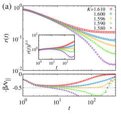
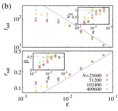
Figure 1: (Color online) (a) Temporal behaviors of $r_{\downarrow}(t)$ near the criticality [$K_{\rm c}=\sqrt{8/\pi}\simeq 1.596$ for Gaussian $g(\omega)$] at $N=819200$. Effective exponent plots in the lower panel indicate the value of $K_{\rm c}$ where $r(t)\sim t^{-\beta/\nu_{\parallel}}$ with $\beta/\nu_{\parallel}=1/2$. (b) Based on critical behaviors $t_{\rm sat}$ and $r_{\rm sat}$ near $\epsilon=0$, two thermodynamic exponents ($\nu_{\parallel}=1,~{}\beta=1/2$) are measured (insets) as $N$ increases. Here data are obtained from the random sampling of $\{\omega_{j}\}$ and $r(0)=1$ (at least 200 ensembles).

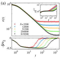
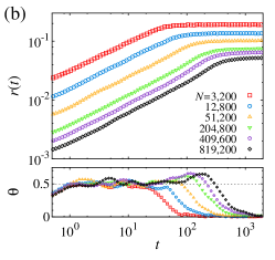
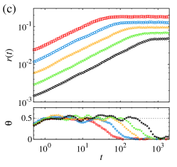
Figure 2: (Color online) For the random sampling of $\{\omega_{j}\}$, $r(t)$ is plotted at $K=K_{\rm c}(T)$ at various $N$ with the corresponding effective exponent ($\beta/\nu_{\parallel}\mbox{~{}or~{}}\theta$) plots: When the KM starts (a) at a coherent [$r(0)=1$] with $\beta/\nu_{\parallel}=1/2$; (b) at an incoherent state [$r(0)\sim N^{-1/2}$] with $\theta=1/2~{}\to~{}3/4$; (c) at the same state as (b) but containing thermal noise ($T=0.1$) with $\theta=1/2$. Note that the same symbol (color) corresponds to the same size as described in (b) unless any other explanations are provided.

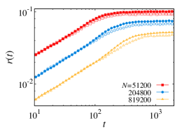
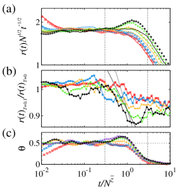
Figure 3: (Color online) The effect of thermal noise on dynamic scaling of $r(t)$ at $K=K_{\rm c}(T)$ is tested for two cases, $T=0.1$ (noisy, open symbols) and $T=0$ (noiseless, filled symbols), at three different $N$ values. (a) The noisy random sampling case (lines for $T=0.1$) is compared to the noiseless case (symbols for $T=0$). (b) The ratio of two cases are plotted. Two straight lines are guides for eyes, of which slopes are -0.15 and -0.25, respectively. Based on our conjecture, it should be the same as $\theta_{T=0.1}-\theta_{T=0}=-1/4$. (c) Scaling collapse of effective exponents in the lower panel of Fig. 2 (b) implies $t_{\rm cross}\sim t_{\rm sat}\sim N^{\bar{z}}$ with $\bar{z}=2/5$. Here we use the same data as those in the upper panel of Fig. 2 (b) and (c).

I Introduction

Collective synchronization of coupled oscillators is a fascinating phenomenon, where non-identical oscillators are spontaneously coherent at the same frequency with identical phase angles with each cycle (or a repeating sequence of phase angles over consecutive cycles) with diverging scales. This cooperative behavior is ubiquitous in real systems from well-known examples, Josephson junction arrays, chemical oscillators and flashing of fireflies old-intro+review , to most recent examples, such as power grids Rohden2012PRL+Doefler2012PNAS+Motter2013NPHYS , chimera states in oscillator networks Martens2013PNAS , and neural networks Takahashi2010PNAS+Kveraga2011PNAS .

From theoretical point of view, such a remarkable phenomenon has also become a central issue as an universal concept in nonlinear science books . Kuramoto introduced a mathematically tractable model of coupled nonlinear oscillators Kuramoto as refining the earlier model by Winfree Winfree . Since then, the Kuramoto model (KM) has played a role as the paradigmatic model of synchronization. The KM is simple but exhibits rich behaviors; among them, the synchronization transition is one of fundamental problems. At the transition, oscillators’ phases are tuned by the critical coupling strength against non-identical natural frequencies, and eventually reach a phase-locked state (frequency entrainment) including in-phase synchronization with exactly the same value.

A continuous synchronization transition in the KM was firstly characterized in the mean-field (MF) picture, and accomplished by solving a self-consistent equation of the order parameter. The MF solution of critical exponents associated with the order parameter ($r\sim\epsilon^{\beta}$) and the correlation volume ($\xi_{v}\sim\epsilon^{-\bar{\nu}}$) were obtained as $\beta=1/2$ and $\bar{\nu}=2$, respectively Kuramoto1984PTPS ; Daido1987JPA , where $\epsilon$ is the reduced control parameter and natural frequencies were randomly assigned from the Gaussian distribution. However, based on the FSS theory and heuristic arguments, the FSS exponent $\bar{\nu}$ has been re-obtained as $\bar{\nu}=5/2$ Hong2004n2005PRE+2007PRL . It was taken into account for size-dependent sample-to-sample fluctuations in natural frequencies, but numerical confirmation was not entirely satisfactory due to finite-size effects. Meanwhile, it has been also reported that thermal noise, quenched disorder of natural frequencies, and link disorder of coupled oscillators, can also be relevant to the value of the FSS exponent Son2010PRE ; Tang2011JSM ; Hong2013PRE .

In the absence of exact solutions, numerical tests are inevitable, which is limited to finite systems related to computing facilities. This issue has long been recognized in phase transitions and critical phenomena. While FSS has played a crucial role in its remedy, it requires the steady-steady limit of finite systems, which takes quite a long computation time in the numerical sense. Up to now, the FSS analysis of phase synchronization has been carried out based on the steady-state limiting data only. So one can naturally pose the following question: What if there are only temporal data available? Is there any systematic approach to deal with them? The answers will be carefully addressed in this paper.

We propose an extended FSS form of the phase order parameter, which provides another comprehensive view of synchronization with the connection of dynamic scaling to FSS near and at the criticality. In particular, we focus on how the order parameter behaves in the true scaling regime before it gets into the steady state, involved with the FSS exponent. Owing to the dynamic scaling analysis, we successfully confirm the theoretical value $\bar{\nu}=5/2$. Moreover, we also show $\bar{\nu}=2$, which is clearly distinct from it in the presence of thermal noise. As a final remark, we discuss the oscillatory behavior of the order parameter in time with two scaling regimes. This occurs when the KM starts at an incoherent state with fluctuation-free natural frequencies by the regular sampling from the Gaussian distribution.

It is well known that dynamic scaling is useful in nonequilibrium systems such as surface growths Barabasi1995 , cluster aggregation models Vicsek1984PRL , and absorbing phase transitions Marro1999 . However, the dynamic scaling analysis in synchronization models has not yet been studied seriously to our knowledge.

The main purpose of this paper is to present dynamic scaling in synchronization and to clarify its universality issue as approaching the critical coupling strength.

This paper is organized as follows: In Sec. II, we briefly review the ordinary KM and the conventional FSS theory of the phase order parameter. In Sec. III, we present the dynamic scaling concept using the extended FSS theory and test it with two completely different initial setups. The validity and the universality issue of dynamic scaling are discussed in Sec. IV with numerical tests of thermal noise and quenched disorder fluctuation. Finally, we conclude in Sec. V with a summary of our findings.

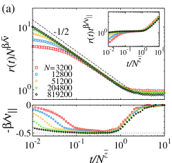
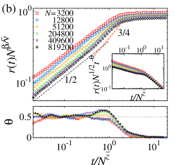
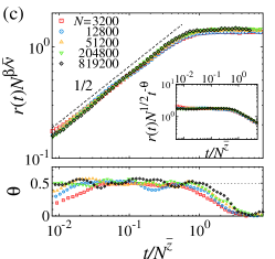
Figure 4: (Color online) Scaling collapse of Fig. 2: In the upper panel, ${\mathcal{F}}(x)=r(t)N^{\alpha}$ is tested as main plots and $f(x)=r(t)N^{\zeta}t^{y}$ as inset plots, where $x\equiv t/N^{\bar{z}}$, $\alpha=\beta/\bar{\nu}$, and $(\zeta,y)=[(0,~{}\beta/\nu_{||})~{}{\rm{for~{}(a)}};~{}(1/2,-\theta)~{}{\rm{~{}for~{}(b)~{}and~{}(c)}}$] at $K=K_{\rm c}(T)$ for various $N$. In the lower panel, the corresponding effective exponents are also plotted using dynamic scaling with the exponent set of ($\beta/\bar{\nu},~{}\bar{z},~{}\beta/\nu_{\parallel}\mbox{~{}or~{}}\theta$): When the system starts (a) at a coherent [$r(0)=1$] with (1/5, 2/5, 1/2); (b) at an incoherent state [$r(0)\sim N^{-1/2}$] with (1/5, 2/5, 3/4); (c) at the same state as (b) but containing thermal noise ($T=0.1$) with (1/4, 1/2, 1/2).

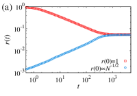
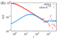
Figure 5: (Color online) The noiseless ($T=0$) case: (a) for the random sampling of $\{\omega_{j}\}$ at $N=102400$ and (b) for the regular sampling of $\{\omega_{j}\}$ at $N=1600$ (relatively small to the random case due to slow relaxation). Here circle (blue) symbols start from an incoherent state and square (red) ones from a coherent state.

II Model

We begin with the KM Kuramoto , a paradigm of random intrinsic frequency oscillators with the all-to-all coupling, which is defined by the set of dynamic equations as

$$\frac{{\rm d}{\phi}_{j}(t)}{{\rm d}{t}}=\omega_{j}+\frac{K}{N}\sum_{k=1}^{N}{\sin\big{(}\phi_{k}(t)-\phi_{j}(t)\big{)}},$$ (1)

where $\phi_{j}(t)$ is the phase of the $j$-th oscillator at time $t$ ($j,k=1,...,N$ for total number of oscillators), $\omega_{j}$ is its time-independent natural frequency that follows the distribution $g(\omega)$, and $K$ is the coupling strength. To observe a second-order (continuous) synchronization transition, we set $g(\omega)$ to be a Gaussian with zero mean and unit variance: $g(\omega)=\frac{1}{\sqrt{2\pi}}\exp(-\frac{\omega^{2}}{2})$. It is well-known that $\{\omega_{j}\}$ in the KM plays a role as quenched disorder and its functional shape, $g(\omega)$, is relevant to the nature of the synchronization transition Pazo2005PRE . As $K$ increases, phase synchronization occurs at the critical coupling strength $K_{\mathrm{c}}=\frac{2}{\pi g(0)}(=\sqrt{8/\pi})$ Kuramoto , which can be quantified by a global complex-valued order parameter:

$$r(t)e^{i\psi(t)}\equiv\frac{1}{N}\sum_{k=1}^{N}e^{i\phi_{k}(t)}.$$ (2)

For the conventional FSS analysis, one collects the order parameter $r$ only after it gets saturated to the steady-state limiting value, where the time-averaged value is also taken, denoted as $\langle r\rangle$, and the sample-averaged value over the different sets of $\{\phi_{j}(0)\}$ at $t=0$ and $\{\omega_{j}\}$ is denoted as $[\langle r\rangle]$. To discuss dynamic scaling in synchronization, we also focus on $r(t)$ (actually $[r(t)]$ used to reduce statistical errors) for the whole regimes from the dynamic state up to the steady state [see Fig. 1 and Fig. 2]. It is already known that $r(t)$ grows exponentially far from the criticality: $r(t)\sim\exp(at)$ before it saturates to $r_{\rm sat}$ for $K\gg K_{\mathrm{c}}$ Strogatz1991JSP . For $K\ll K_{\mathrm{c}}$, it does not grow enough but fluctuates near 0 as much as $O(N^{-1/2})$. Moreover, the relaxation and decay mechanism below $K_{\mathrm{c}}$ had been discussed with the similarity of Landau damping Strogatz1992PRL . So the naturally posed question is how it evolves near and at $K=K_{\mathrm{c}}$.

In this paper, we trace the formation of synchronized clusters and the cooperative behavior with time in the vicinity of $K_{\rm c}~{}(\epsilon\equiv\frac{K-K_{\rm c}}{K_{\rm c}}=0)$, as the correlation volume $\xi_{v}$ and the correlation time $\tau$ become very large, compared to the subcritical regime $(\epsilon<0)$ and the supercritical regime $(\epsilon>0)$, which algebraically decay as $\xi_{v}\sim|\epsilon|^{-\bar{\nu}}$ and $\tau\sim|\epsilon|^{-\nu_{\parallel}}$, respectively. However, $\xi_{v}\to N$ in finite systems at $\epsilon=0$. As a result, $\tau\sim N^{\bar{z}}$ with $\bar{z}={\nu_{\parallel}}/{\bar{\nu}}$. Therefore, we are able to estimate the FSS exponent $\bar{\nu}$ using both temporal and static properties of the order parameter from either $\bar{z}$ of the saturation time ($t_{\rm sat}\sim\tau\sim N^{\bar{z}})$ or $\alpha\equiv\beta/\bar{\nu}$ of the saturation value ($r_{\rm sat}\sim N^{-\alpha}$) as well as the critical threshold $K_{\mathrm{c}}$ in two independent ways.

All numerical data presented here are obtained using the 4th order Runge-Kutta method and $\mathrm{d}t$=0.01, which are averaged over at least 500 samples, except Fig. 1 in which 200 ensemble is enough.

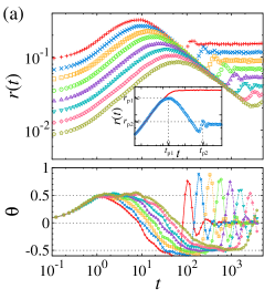
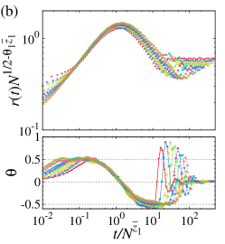
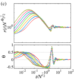
Figure 6: (Color online) For the noiseless regular sampling of $\{\omega_{j}\}$, dynamic scaling is tested at various $N$. (a) Temporal behaviors of $r(t)$ (upper panel) and the corresponding effective exponent (lower panel) are plotted, where $N=100,~{}200,~{}\cdots,~{}12800$ from top to bottom. In the inset, the random case (red, line) is compared with the regular one (blue, symbol) with $N=800$. Two sets of data collapse of $r(t)$ are shown for two different scaling regimes as well as those of effective exponents (b) near the first peak with $\theta_{1}=1/2$ and $\bar{z}_{1}=2/5$, and (c) near and after the second peak with $\theta_{2}=-1/2$ and $\bar{z}_{2}=4/5$.

III Dynamic Scaling

When a system exhibits self-similar dynamics at the criticality, one can focus on dynamic scaling with a proper initial setup.

We revisit phase synchronization in the ordinary KM since the values of $K_{\rm c}$ and $\beta$ are exactly known. Owing to that fact, we easily test various properties and confirm the existence of dynamic scaling. However, we note that the dynamic scaling analysis is also powerful to indicate the location of $K_{\rm c}$ [see Fig. 1]. Furthermore, we discuss the universality issue in synchronization, related to the relevance of thermal and link-disorder fluctuations of oscillators against two different sampling methods of natural frequencies.

Two different initial conditions of the KM are chosen to start either at a fully coherent state [where $\phi_{j}(0)=\phi_{o}$: an arbitrary angle, independent of $j$, so $r(0)=1$] or at an incoherent state [where $\phi_{j}(0)\in[0,2\pi)$ is random, so $r(0)\sim N^{-1/2}$]. For a given value of $K$, $r(t)$ evolves either exponentially or algebraically up to $\tau\equiv t_{\rm sat}$, which is also subject to the system size $N$.

Based on the FSS theory and thermodynamic limiting results as $N\to\infty$: $t_{\rm sat}\sim\epsilon^{-\nu_{\parallel}}$ with $\nu_{\parallel}=1$ and $r_{\rm sat}\sim\epsilon^{\beta}$ with $\beta=1/2$, which is also numerically confirmed in Fig. 1. So the extended FSS to dynamic scaling can be rewritten near and at $\epsilon=0$ as

$$r(t,N,\epsilon)=b^{-\alpha}r_{b}(b^{-\bar{z}}t,b^{-1}N,b^{1/\bar{\nu}}\epsilon),$$ (3)

where $b$ is an arbitrary scaling factor and $\alpha\equiv\beta/\bar{\nu}$. In the steady-state limit ($t\to\infty$), Eq. (3) is exactly the same as the earlier FSS form, $r(\epsilon,N)=N^{-\alpha}f(\epsilon N^{1/\bar{\nu}})$ Hong2004n2005PRE+2007PRL .

Equation (3) can also be rewritten as the dynamic scaling form with two variables, $t$ and $N$, as $N\to\infty$ ($b=t^{1/\bar{z}}$) or as $t\to\infty$ ($b=N$):

$$r(t,N)=t^{-\alpha/\bar{z}}f(t/N^{\bar{z}})=N^{-\alpha}\mathcal{F}(t/N^{\bar{z}}),$$ (4)

which is numerically confirmed (see Figs. 2-4). Here $\alpha=\beta/\bar{\nu}$ from $r_{\rm sat}$ and $\bar{z}=\nu_{\parallel}/\bar{\nu}$ from $t_{\rm sat}$.

To confirm that the transition is continuous and discuss how the initial setup affects dynamic scaling at the transition in detail, two completely different configurations are considered, which correspond to Fig. 4 (a) and (b) for the ordinary KM starting from a fully coherent state and from a random (incoherent) state, respectively.

The below form of dynamic scaling describes that the KM initially starts at $r(0)=1$. As time elapses, the order parameter decays as a power law, denoted as $r_{\downarrow}(t,N)$:

$$r_{\downarrow}(t,N) = t^{-\alpha/\bar{z}}f_{\downarrow}(t/N^{\bar{z}})=N^{-\alpha}\mathcal{F}_{\downarrow}(t/N^{\bar{z}})$$ (5)

$$\sim \begin{cases}t^{-\alpha/\bar{z}}&\text{for }t_{\times}<t\ll t_{\rm sat}(\sim N^{\bar{z}}),\\ N^{-\alpha}&\text{for }t\gg t_{\rm sat},\\ \end{cases}$$

where $f_{\downarrow}(x)$ is constant for $x\ll 1$ in the true scaling regime ($t_{\times}<t\ll t_{\rm sat}$) after the transient regime ($t<t_{\times}$ when the initial condition effect exists; $t_{\times}$ is independent of $N$ in general), and $f_{\downarrow}(x)\sim x^{\alpha/\bar{z}}$ for $x\gg 1$ in the saturation regime ($t\gg t_{\rm sat}\sim N^{\bar{z}}$; when the system-size dependence only exists) [see Fig. 2 (a) and Fig. 4 (a)].

If one chooses an initial configuration starting at an incoherent state with $N$-dependent randomness [$r(0)\sim N^{-1/2}$], the order parameter increases in a trivial power law to wash out such randomness after the transient regime, and then it exhibits true scaling. Therefore, Eq. (5) should be modified due to $N$-dependent trivial offset ($\sim N^{-1/2}$) and trivial temporal scaling ($\sim t^{1/2}$), denoted as $r_{\uparrow}$ for convenience, as follows:

$$r_{\uparrow}(t,N) = N^{-1/2}t^{\theta}f_{\uparrow}(t/N^{\bar{z}})=N^{-\alpha}\mathcal{F}_{\uparrow}(t/N^{\bar{z}})$$ (6)

$$\sim \begin{cases}N^{-1/2}t^{1/2}&\text{for }t_{\times}<t<t_{\rm cross},\\ N^{-1/2}t^{\theta}&\text{for }t_{\rm cross}\ll t\ll t_{\rm sat},\\ N^{-\alpha}&\text{for }t\gg t_{\rm sat},\\ \end{cases}$$

where $f_{\uparrow}(x)$ is constant for $x_{*}(\equiv t_{\rm cross}/N^{\bar{z}})\ll x\ll 1$ in the true scaling regime, and $f_{\uparrow}(x)\sim x^{({\alpha-\frac{1}{2}})/\bar{z}}$ for $x\gg 1$ in the saturation regime [see Fig. 2 (b),(c) and Fig. 4 (b),(c)].

Figure 2 (b) [see Fig. 4 (b) as well] shows very long transient trivial scaling in the time evolution of $r(t)$ due to random phases at $t=0$, $r(t)\sim N^{-1/2}t^{1/2}$. This lasts up to $t_{\rm cross}$ until the random initial condition effect is washed out and the system exhibits true scaling with $N^{-1/2}t^{\theta}$. In order to resolve this universality issue, one needs to find the crossover time $t_{\mathrm{cross}}$ accurately as well as the true scaling behavior. It is definitely not an easy task and sometimes extremely tricky if the window of two consecutive scaling regimes is narrow because one scaling interferes with the other one.

From the fact that at a continuous transition the steady state should be the same, irrespective of initial setups [see Fig. 5 (a)], we derive a scaling relation among $\alpha(=\beta/\bar{\nu}),~{}\theta,$ and $\bar{z}(=\nu_{\parallel}/\bar{\nu})$ as $\frac{1}{2}-\theta\bar{z}=\alpha$ in $r_{\rm sat}\sim N^{-\alpha},~{}r_{\uparrow}(t)N^{1/2}\sim t^{\theta},$ and $t_{\rm sat}\sim N^{\bar{z}}$, respectively. This is equivalent to $\theta=(\frac{1}{2}-\alpha)/\bar{z}=(\frac{\bar{\nu}}{2}-\beta)/\nu_{\parallel}$. Hence, $r_{\uparrow}(t)$ for the random sampling of $\{\omega_{j}\}$ with the random choice of $\{\phi_{j}(0)\}\in[0,2\pi)$ is characterized by two different length scales, unlike the conventional temporal behavior in a simple power-law manner. It is because it is involved with two different dynamic exponents, which is attributed to the finite-size effect and the crossover from $t^{1/2}$ to $t^{3/4}$ at $t_{\rm cross}$ as time elapses.

The true dynamic exponent $\bar{z}$ related to the true FSS exponent $\bar{\nu}$ in the long-time regime after the crossover yields $\tau\sim N^{\bar{z}}$ where $\bar{z}=1/\bar{\nu}=2/5$ with $\nu_{\parallel}=1$ in networks, only observed in sufficiently large system sizes. Otherwise, the crossover scaling of $\bar{z}=1/\bar{\nu}=1/2$ is only detected, which is related to thermal noise [see Fig. 3]. This anomalous dynamic scaling of $r_{\uparrow}(t)$ is resolved with thermal noise $\eta_{j}(t)$ using the modified KM Son2010PRE :

$$\frac{{\rm d}{\phi}_{j}(t)}{{\rm d}{t}}=\omega_{j}+\frac{K}{N}\sum_{k=1}^{N}{\sin\big{(}\phi_{k}(t)-\phi_{j}(t)\big{)}}+\eta_{j}(t),$$ (7)

where $\langle\eta_{j}(t)\rangle=0$ and $\langle\eta_{j}(t)\eta_{k}(t^{\prime})\rangle=2T\delta_{jk}\delta(t-t^{\prime})$. In the modified KM, we observe that the conventional dynamic scaling governed by random fluctuations with $\bar{z}=1/\bar{\nu}=1/2$ as expected [see Fig. 2 (c) and Fig. 4 (c)].

Using the KM with various settings, we discuss the universality of the dynamic exponent in true scaling.

IV Effects of Noise and Disorder

In order to discuss the validity of our conjecture on the dynamic scaling form, it is necessary to test the relevance of thermal noise and the type of disorder in the KM as discussed in the FSS theory Son2010PRE ; Tang2011JSM ; HP+Hong . In the presence of thermal noise, it is always relevant, irrespective of disorder type. So it changes the value of $\bar{\nu}=1/\bar{z}$ with $\nu_{\parallel}=1$ from $\bar{\nu}=5/2$ to $\bar{\nu}=2$ (see Table 1).

Compared to the case of the noiseless ($T=0$) random sampling [see Fig. 2 (b) and Fig. 4 (b)], $r_{\uparrow}(t)$ for the noisy case exhibits clean dynamic scaling [see Fig. 2 (c) and Fig. 4 (c)] with $\bar{\nu}=2$. This distinction of these two cases plays a key role in detecting the true scaling regime ($t\gg t_{\rm cross}$) for the case of noiseless random sampling [see Fig. 3]. However, the window of the true scaling regime is somehow quite short (at most one decade) and hardly observable in smaller systems, implying that the case of noiseless random sampling is hardly distinguishable with the noisy one in numerical senses unless $N$ is big enough. This is why some numerical results reported $\bar{\nu}=2$ (not $\bar{\nu}=5/2$) even for the noiseless case.

Based on our extensive numerical simulation results, $r_{\uparrow}(t)$ in bigger systems at least $N\geq 204,800$ exhibit their own true scaling regime clearly [see Fig. 4(b),(e), and Fig. 3]. This is why one cannot observe true scaling in smaller systems ($N<N_{\mathrm{cross}}$), which $t_{\rm cross}(N)\geq t_{\rm sat}(N)$ due to finite-size corrections to scaling. Note that $N_{\mathrm{cross}}=O(10^{5})$ can be estimated from $r_{\mathrm{sat}}(\epsilon,N)=N^{-1/5}f(\epsilon N^{2/5})$ and $r_{\mathrm{sat}}\ll 1$ at $\epsilon=0$.

To discuss the relevance of natural frequency sampling (quenched disorder type) in dynamic scaling as well as the initial setups, we revisit the KM in the absence of thermal noise. If $\{\omega_{j}\}$ is regularly generated by $\omega_{j}=\sqrt{2}\mathrm{erf}^{-1}\left(-1+\frac{2j-1}{N}\right)$, it plays a role as “sample-to-sample fluctuation-free” quenched disorder in the system.

For this regular sampling [see Fig. 6], $r_{\uparrow}(t)$ exhibits very interesting damped oscillation, rather than anomalous crossover scaling for the random sampling case. However, if a system exhibits a continuous phase transition, the steady-state limit should be independent of initial setups. Through Fig. 5, we confirm that the order parameter for the noiseless ($T=0$) case starting two completely different initial setups has the same value in the steady-state, and we find that the anomalous oscillatory behavior exists for the regular sampling of $\{\omega_{j}\}$ starting with an incoherent state. The comparison with the noisy case ($T\neq 0$) is shown in Fig. 7. In the inset of Fig. 6 (a), the heights of two largest peaks at the corresponding times are taken as indicators, respectively.

Based on numerical tests as shown in Fig. 6 (b),(c) and Fig. 8 (e),(f), we find that $(r_{\mathrm{p}1}\sim N^{-\alpha_{1}},~{}t_{\mathrm{p}1}\sim N^{\bar{z}_{1}})$ at the first largest one and $(r_{\mathrm{p}2}\sim N^{-\alpha_{2}},~{}t_{\mathrm{p}2}\sim N^{\bar{z}_{2}})$ at the second largest one, with ($\alpha_{1}=3/10$, $\bar{z}_{1}=2/5$) with $\theta_{1}=1/2$ for the first scaling regime and ($\alpha_{2}\simeq 2/5$, $\bar{z}_{2}\simeq 4/5$) with $\theta_{2}\simeq-1/2$ for the second one. We conjecture the following scaling relations: $\alpha_{1}=1/2-\theta_{1}\bar{z}_{1}$ and $\alpha_{2}=-\theta_{2}\bar{z}_{2}$. As a result, Eq. (6) should be modified to the following two forms:

$$r_{\uparrow,\mathrm{p}1}(t,N) = N^{-1/2}t^{\theta_{1}}f_{\uparrow,\mathrm{p}1}(t/N^{\bar{z}_{1}})=N^{-\alpha_{1}}\mathcal{F}_{\uparrow,\mathrm{p}1}(t/N^{\bar{z}_{1}})\sim\begin{cases}N^{-1/2}t^{\theta_{1}}&\text{for }t_{\times}<t\ll t_{\mathrm{p}1}\sim N^{\bar{z}_{1}},\\ N^{-\alpha_{1}}&\text{at }t=t_{\mathrm{p}1}\sim N^{\bar{z}_{1}},\\ \end{cases}$$ (8)

$$r_{\uparrow,\mathrm{p}2}(t,N) = t^{\theta_{2}}f_{\uparrow,\mathrm{p}2}(t/N^{\bar{z}_{2}})=N^{-\alpha_{2}}\mathcal{F}_{\uparrow,\mathrm{p}2}(t/N^{\bar{z}_{2}})\sim\begin{cases}t^{\theta_{2}}&\text{for }t_{\mathrm{p}1}\ll t\ll t_{\mathrm{p}2}\sim N^{\bar{z}_{2}},\\ N^{-\alpha_{2}}&\text{for }t\gg t_{\mathrm{p}2},\end{cases}$$ (9)

where $f_{\uparrow,\mathrm{p}1}(x)$ is constant for $x\ll 1$, $f_{\uparrow,\mathrm{p}1}(x)\sim x^{-\theta_{1}}$ for $x\gg 1$ and $f_{\uparrow,\mathrm{p}2}(x)$ is constant for $x\ll 1$, $f_{\uparrow,\mathrm{p}2}(x)\sim x^{-\theta_{2}}$ for $x\gg 1$. Figure 6 (b) and (c) correspond to the scaling function ${\mathcal{F}}_{\uparrow}(t/N^{\bar{z}})=r_{\uparrow}(t)N^{\alpha}$ in Table 1.

Unlike the random sampling of $\{\omega_{j}\}$, the regular one has not been fully understood except for the nontrivial value of the FSS exponent ($\bar{\nu}\simeq 5/4$ reported in Son2010PRE ; Tang2011JSM ; Hong2013PRE ). Our dynamic scaling results would give a hint to find the correct value of $\bar{\nu}$ but also address how and when the effect of initial condition is washed out in $r(t)$ [see Fig. 5].

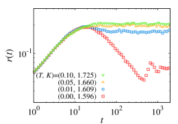
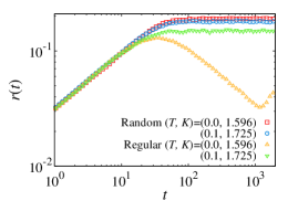
Figure 7: (Color online) Critical behaviors of $r_{\uparrow}(t)$ at $K=K_{\rm c}(T)$: at $N=800$ for the regular sampling of $\{\omega_{j}\}$ for the upper panel and at $N=3200$ for four different cases that are described in Table 1 with 1000 ensembles for the lower panel. However, the steady-state limiting value in finite systems, $r_{\rm sat}(N)$, seems to depend on the value of $T$ for the regular sampling case of $\{\omega_{j}\}$ if the effect of $T$ is relatively small, compared to the effect of $N$.

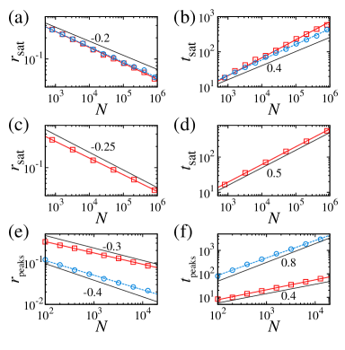
Figure 8: (Color online) FSS data analysis for the saturated values with $r_{\rm sat}\sim N^{-\alpha}$ and $t_{\rm sat}\sim N^{\bar{z}}$: (a) and (b) for the noiseless random case, where blue circle (red square) symbols represent the data starting at a fully coherent (incoherent) state, and the slope sets $(-\alpha,~{}\bar{z})$ of naive fitting lines correspond to (-0.22, 0.44) for circles and (-0.23, 0.51) for squares; (c) and (d) for the noisy random case with $T=0.1$, where blue square symbols represent the data starting at an incoherent state, and the slope set of naive fitting lines corresponds to (-0.24, 0.50); (e) and (f) for the noiseless regular case, where red square (blue circle) symbols represent the scaling properties of the first (second) peak in $r_{\uparrow}(t)$ [described in the inset of Fig. 6(a)], and the slope sets of naive fitting lines correspond to (-0.27, 0.42) for squares and (-0.35, 0.74) for circles.

Table 1: All critical exponents are summarized with the earlier FSS results and our conjecture for dynamic scaling. For the noiseless regular sampling of $\{\omega_{j}\}$, $\theta(t)=1/2$ for $t\ll t_{\mathrm{p}1}(\sim N^{\bar{z}_{1}}$ with $\bar{z}_{1}\simeq 2/5$); -1/2 for $t_{\mathrm{p}1}\ll t\ll t_{\mathrm{p}2}(\sim N^{\bar{z}_{2}}$ with $\bar{z}_{2}\simeq 4/5$) [see Fig. 6 and Fig. 8]. For all the cases, the scaling function ${\mathcal{F}}_{\uparrow}(x)={\rm constant}$ for $x\gg 1$, where $x\equiv t/N^{\bar{z}}$.

Sampling	Noise	Steady State	Dynamic State	Dynamic Scaling	Scaling Function
$\{\omega_{j}\}$ from $g(\omega)$	$T$	$(\beta/\bar{\nu},~{}1/\bar{\nu})$	$(\beta/\nu_{\parallel},~{}\theta,~{}\bar{z})$	starting at $r(0)~{}N^{-1/2}$	${\mathcal{F}}_{\uparrow}(x)$
random	$T=0$	(1/5, 2/5)	(1/2, 3/4, 2/5)	$r_{\uparrow}(N,t)=N^{-2/5}{\mathcal{F}}_{\uparrow}(t/N^{2/5})$	$~{}x^{3/4}{\rm~{}for~{}}x_{\rm cross}\ll x\ll 1$
	$T\neq 0$	(1/4, 1/2)	(1/2, 1/2, 1/2)	$r_{\uparrow}(N,t)=N^{-1/4}{\mathcal{F}}_{\uparrow}(t/N^{1/2})$	$~{}x^{1/2}{\rm~{}for~{}}x_{\times}\ll x\ll 1$
regular	$T=0$	(2/5, 4/5)∗	(1/2, 1/2, 2/5)	$r_{\uparrow,{\rm p1}}(N,t)=N^{-3/10}{\mathcal{F}}_{\uparrow,{\rm p1}}(t/N^{2/5})$	$~{}x^{1/2}{\rm~{}for~{}}x_{\times}\ll x\ll x_{\rm p1}$
			(1/2, -1/2, 4/5)	$r_{\uparrow,{\rm p2}}(N,t)=N^{-2/5}{\mathcal{F}}_{\uparrow,{\rm p2}}(t/N^{4/5})$	$~{}x^{-1/2}{\rm~{}for~{}}x_{\rm p1}\ll x\ll x_{\rm p2}$
	$T\neq 0$	(1/4, 1/2)	(1/2, 1/2, 1/2)	$r_{\uparrow}(N,t)=N^{-1/4}{\mathcal{F}}_{\uparrow}(t/N^{1/2})$	$~{}x^{1/2}{\rm~{}for~{}}x_{\times}\ll x\ll 1$

Furthermore, the origin of oscillatory behaviors in dynamic scaling is still under investigation. Figure 7 shows that it is completely gone once thermal noise is turned on. Most recently, it has been also reported in Hong2013PRE that link fluctuations of oscillator networks generate effective fluctuations of natural frequencies, which means the absence of oscillatory behaviors once random fluctuations in links of oscillator networks are considered. Such a change is also numerically observed. A more detailed investigation for dynamic scaling unpublished will be provided elsewhere to complete the discussion of the universality issue in synchronization as well as the transition nature against the distribution type of natural frequencies.

Finally, we discuss how the strength of thermal noise ($T$) affects dynamic scaling of $r_{\uparrow}(t)$ at $K=K_{\rm c}(T)$, which is based on Fig. 7. Once we turn on thermal noise, the oscillatory behavior for the noiseless case is washed out. For four different cases that are described in Table 1, we also compare one with another. Moreover, all the FSS data analysis and dynamic scaling results are summarized in Fig. 8 and Table 1 in detail manner as possible.

V Summary and Discussions

In conclusion, we have systematically explored dynamic scaling of synchronization in the Kuramoto model, and investigated scaling relations between our results and the earlier FSS ones. We also found that dynamic scaling properties can also clearly locate the critical coupling strength of synchronization and estimate the values of critical exponents. As a final remark, we addressed how the initial phases of oscillators and the generation method of natural frequency sequences affect dynamic scaling and the FSS exponent, which were numerically confirmed.

The merit of dynamic scaling, similar to the earlier work on the short-time behavior of the two-dimensional $\phi^{4}$ theory Zheng1999PRL , is to provide another comprehensive view of synchronization by the time evolution of the order parameter before the system reaches the steady state against various initial setups. This offers a guideline how to analyze a phase synchronization transition in finite systems without any steady-state limiting results.

We believe that dynamic scaling provides rich information in analyzing real systems, including the transition nature and the universality issue.

References

- (1) P. Barbara, A.B. Cawthorne, S.V. Shitov, and C.J. Lobb, Phys. Rev. Lett. 82, 1963 (1999); I.Z. Kiss, Y.M. Zhai, and J.L. Hudson, Science 296, 1676 (2005); J.A. Acebrón et. al., Rev. Mod. Phys. 77, 137 (2005).
- (2) M. Rohden, A. Sorge, M. Timme, and D. Witthaut, Phys. Rev. Lett. 109, 064101 (2012); F. Dörfler, M. Chertkov, and F. Bulllo, PNAS 110, 2005 (2012); A.E. Motter, S.A. Myers, M. Anghel, and T. Nishikawa, Nat. Phys. 9, 191 (2013).
- (3) E.A. Martens, S. Thutupalli, A. Fourriére, and O. Hallastchek, PNAS 110, 10563 (2013).
- (4) N. Takahashi et al., PNAS 107, 10244 (2010); K. Kveraga et al., PNAS 108, 3389 (2011).
- (5) A.S. Pikovsky, M. Rosenblum, and J. Kurths, Synchronization: A Universal Concept in Nonlinear Science, Cambridge Nonlinear Science Series (Cambridge University Press, Combridge, England, 2001); G.V.Osipovsky, J. Kurths, and C. Zhou, Synchronization in Osillatory Networks, Springer Series in Synergetics (Springer, Berlin, 2007); S. Boccaletti, The Synchronized Dynamics of Complex Systems, edited by A.C. Luo and G. Zaslavsky, Monograph Series on Nonlinear Science and Complexity, Vol. 6 (Elsevier Science, Amsterdam, 2008).
- (6) Y. Kuramoto in Proceedings of the International Symposium on Mathematical Problems in Theoretical Physics, Lecture Notes in Physics, Vol. 39, edited by H. Araki (Springer-Verlag, Berlin, 1975); Chemical Oscillations, Waves, and Turbulence (Springer-Verlag, Berlin, 1984).
- (7) A.T. Winfree, J. Theor. Biol. 16, 15 (1967); The Geometry of Biological Time (Springer-Verlag, Berlin, 1980).
- (8) Y. Kuramoto, Prog. Theor. Phys. Suppl. 79, 223 (1984).
- (9) H. Daido, J. Phys. A.:Math.Gen. 20, L629 (1987).
- (10) H. Hong, H. Park, and M.Y. Choi, Phys. Rev. E 70, 045204(R) (2004); ibid. 72, 036217 (2005); H. Hong, H. Chaté, H. Park, and L.-H. Tang, Phys. Rev. Lett. 99, 184101 (2007).
- (11) S.-W. Son and H. Hong, Phys. Rev. E 81, 061125 (2010).
- (12) L.-H. Tang, J. Stat. Mech.: Theor. Exp. P01034 (2011).
- (13) H. Hong, J. Um, and H. Park, Phys. Rev. E 87, 042105 (2013).
- (14) A.-L. Barabási and H. E. Stanley, Fractal Concepts of Surface Growth (Cambridge University Press, Cambridge, 1995).
- (15) T. Vicsek and F. Family, Phys. Rev. Lett. 52, 1669 (1984).
- (16) J. Marro and R. Dickman, Nonequilibrium Phase Transitions in Lattice Models (Cambridge University Press, Cambridge, 1999).
- (17) D. Pazó, Phys. Rev. E 72, 046211 (2005).
- (18) S.H. Strogatz and R.E. Mirollo, J. Stat. Phys. 63, 613 (1991).
- (19) S.H. Strogatz, R.E. Mirollo, P.C. Matthews, Phys. Rev. Lett. 68, 2730 (1992).
- (20) H. Park and H. Hong (private communication).
- (21) C. Choi, D. Kim, and M. Ha (unpublished data).
- (22) B. Zheng, M. Schulz, and S. Trimper, Phys. Rev. Lett. 82, 1891 (1999).