Scattering and transport properties of tight-binding random networks

Abstract

We study numerically scattering and transport statistical properties of tight-binding random networks characterized by the number of nodes $N$ and the average connectivity $\alpha$. We use a scattering approach to electronic transport and concentrate on the case of a small number of single-channel attached leads. We observe a smooth crossover from insulating to metallic behavior in the average scattering matrix elements $\left\langle|S_{mn}|^{2}\right\rangle$, the conductance probability distribution $w(T)$, the average conductance $\left\langle T\right\rangle$, the shot noise power $P$, and the elastic enhancement factor $F$ by varying $\alpha$ from small ($\alpha\to 0$) to large ($\alpha\to 1$) values. We also show that all these quantities are invariant for fixed $\xi=\alpha N$. Moreover, we proposes a heuristic and universal relation between $\left\langle|S_{mn}|^{2}\right\rangle$, $\left\langle T\right\rangle$, and $P$ and the disorder parameter $\xi$.

I Introduction and model

During the last three decades there has been an increasing number of papers devoted to the study of random graphs and complex networks, in view of the fact that they describe systems in many knowledge areas: from maths and physics to finance and social sciences, passing through biology and chemistry BA99 ; S01 ; AB02 ; B13 . In particular, some of those works report studies of spectral and eigenfunction properties of complex networks; see for example Refs. DR93a ; ZX00 ; DR93b ; GGS05 ; SKHB05 ; BJ07a ; BJ07b ; F02 ; DGMS03 ; GT06a ; GT06b ; EK09 ; HS11 ; AMM . That is, since complex networks composed by nodes and the bonds joining them can be represented by sparse matrices, it is quite natural to ask about the spectral and eigenfunction properties of such adjacency matrices. Then, in fact, studies originally motivated on physical systems represented by Hamiltonian sparse random matrices RB88 ; RD90 ; FM91 ; EE92 ; JMR01 can be directly applied to complex networks.

In contrast to the numerous works devoted to study spectral and eigenfunction properties of complex netwoks, to our knowledge, just a few focus on some of their scattering and transport properties MPB07a ; MPB07b ; XLL08 ; SRS10 ; PW13 . So, in the present work we study numerically several statistical properties of the scattering matrix and the electronic transport across disordered tight-binding networks described by sparse real symmetric matrices. We stress that we use a scattering approach to electronic transport; see for example MK04 . In addition, we concentrate on the case of a small number of attached leads (or terminals), each of them supporting one open channel. We also note that tight-binding complex networks have also been studied in Refs. DR93a ; ZX00 ; GT06a ; GT06b .

The tight-binding random networks we shall study here are described by the tight-binding Hamiltonian

$$H=\sum^{N}_{n=1}h_{nn}|n\rangle\langle n|+\sum^{N}_{n=1}\sum^{N}_{m=1}h_{nm}\left(|n\rangle\langle m|+|m\rangle\langle n|\right)\ ,$$ (1)

where $N$ is the number of nodes or vertexes in the network, $h_{nn}$ are on-site potentials and $h_{nm}$ are the hopping integrals between sites $n$ and $m$. Then we choose $H$ to be a member of an ensemble of $N\times N$ sparse real symmetric matrices whose nonvanishing elements are statistically independent random variables drawn from a normal distribution with zero mean $\left\langle h_{nm}\right\rangle=0$ and variance $\left\langle|h_{nm}|^{2}\right\rangle=(1+\delta_{nm})/2$. As in Refs. AMM ; JMR01 , here we define the sparsity of $H$, $\alpha$, as the fraction of the $N(N-1)/2$ nonvanishing off-diagonal matrix elements. I.e., $\alpha$ is the network average connectivity. Thus, our random network model corresponds to an ensemble of adjacency matrices of Erdős-Rényi–type random graphs ER59 ; AB02 ; note1 .

Notice that with the prescription given above our network model displays maximal disorder since averaging over the network ensemble implies average over connectivity and over on-site potentials and hopping integrals. With this averaging procedure we get rid off any individual network characteristic (such as scars SK03 which in turn produce topological resonances GSS13 ) that may lead to deviations from random matrix theory (RMT) predictions which we use as a reference. I.e., we choose this network model to retrieve well known random matrices in the appropriate limits: a diagonal random matrix is obtained for $\alpha=0$ when the nodes in the network are isolated, while a member of the Gaussian Orthogonal Ensemble (GOE) is recovered for $\alpha=1$ when the network is fully connected.

However, it is important to add that the maximal disorder we consider is not necessary for a graph/network to exhibit universal RMT behavior. In fact: (i) It is well known that tight-binding cubic lattices with on-site disorder (known as the three-dimensional Anderson model 3DAM ), forming networks with fixed regular connectivity having a very dilute Hamiltonian matrix, show RMT behavior in the metallic phase (see for example Refs. metallic1 ; metallic2 ). (ii) It has been demonstrated numerically and theoretically that graphs with fixed connectivity show spectral spectral ; TS01 and scattering PW13 ; scattering universal properties corresponding to RMT predictions, where in this case the disorder is introduced either by choosing random bond lengths spectral ; PW13 ; scattering (which is a parameter not persent in our network model) or by randomizing the vertex-scattering matrices TS01 (somehow equivalent to consider random on-site potentials). Moreover, some of the RMT properties of quantum graphs have already been tested experimentally by the use of small ensembles of small microwave networks with fixed connectivity Sirko . (iii) Complex networks having specific topological properties (such as small-world and scale-free networks, among others), where randomness is applied only to the connectivity, show signatures of RMT behavior in their spectral and eigenfunction properties BJ07a ; GT06a ; MPB07a .

The organization of this paper is as follows. In the next section we define the scattering setup as well as the scattering quantities under investigation and provide the corresponding analytical predictions from random scattering-matrix theory for systems with time-reversal symmetry. These analytical results will be used as a reference along the paper. In Section III we analyze the average scattering matrix elements $\left\langle|S_{mn}|^{2}\right\rangle$, the conductance probability distribution $w(T)$, the average conductance $\left\langle T\right\rangle$, the shot noise power $P$, and the elastic enhancement factor $F$ for tight-binding networks as a function of $N$ and $\alpha$. We show that all scattering and transport quantities listed above are invariant for fixed $\xi$. Moreover, we propose a heuristic and universal relation between $\left\langle|S_{mn}|^{2}\right\rangle$, $\left\langle T\right\rangle$, and $P$ and the disorder parameter $\xi$. Finally, Section IV is left for conclusions.

II The scattering setup and RMT predictions

We open the isolated samples, defined above by the tight-binding random network model, by attaching $2M$ semi-infinite single channel leads. Each lead is described by the one-dimensional semi-infinite tight-binding Hamiltonian

$$H_{\mbox{\tiny lead}}=\sum^{-\infty}_{n=1}(|n\rangle\langle n+1|+|n+1\rangle\langle n|)\ .$$ (2)

Using standard methods one can write the scattering matrix ($S$-matrix) in the form MW69

$$S(E)=\left(\begin{array}[]{cc}r&t^{\prime}\\ t&r^{\prime}\end{array}\right)={\bf 1}-2i\sin(k)\,{\cal W}^{\,T}(E-{\cal H}_{\rm eff})^{-1}{\cal W}\ ,$$ (3)

where $t$, $t^{\prime}$, $r$, and $r^{\prime}$ are $M\times M$ transmission and reflection matrices; ${\bf 1}$ is the $2M\times 2M$ unit matrix, $k=\arccos(E/2)$ is the wave vector supported in the leads, and ${\cal H}_{\rm eff}$ is an effective non-hermitian Hamiltonian given by

$${\mathcal{H}}_{\rm eff}=H-e^{ik}{\cal W}{\cal W}^{\,T}\ .$$ (4)

Here, ${\cal W}$ is an $N\times 2M$ matrix that specifies the positions of the attached leads to the network. However, in the random network model we are studying here all nodes are equivalent; so, we attach the $2M$ leads to $2M$ randomly chosen nodes. The elements of ${\cal W}$ are equal to zero or $\epsilon$, where $\epsilon$ is the coupling strength. Moreover, assuming that the wave vector $k$ do not change significantly in the center of the band, we set $E=0$ and neglect the energy dependence of ${\mathcal{H}}_{\rm eff}$ and $S$.

Since in the limit $\alpha=1$ the random network model reproduces the GOE, in that limit we expect the statistics of the scattering matrix, Eq. (3), to be determined by the Circular Orthogonal Ensemble (COE) which is the appropriate scattering matrix ensemble for internal systems $H$ with time reversal symmetry. Thus, below, we provide the statistical results for the $S$-matrix and the transport quantities to be analyzed in the following sections, assuming the orthogonal symmetry. In all cases, we also assume the absence of direct processes (also known as perfect coupling condition), i.e., $\langle S\rangle=0$.

We start with the average of the $S$-matrix elements. It is known that

$$\left\langle|S_{mn}|^{2}\right\rangle_{\mbox{\tiny COE}}=\frac{1+\delta_{mn}}{2M+1}\ ,$$ (5)

where $\left\langle\cdot\right\rangle$ means ensemble average over the COE.

Within a scattering approach to the electronic transport, once the scattering matrix is known one can compute the dimensionless conductance Landauer

$$T={\mbox{Tr}}(tt^{\dagger})=\sum_{m}\sum_{n}|t_{mn}|^{2}$$

and its distribution $w(T)$. For $M=1$, i.e. considering two single-channel leads attached to the network, $w(T)$ is given by

$$w(T)_{\mbox{\tiny COE}}=\frac{1}{2\sqrt{T}}\ ,$$ (6)

while for $M=2$,

$$w(T)_{\mbox{\tiny COE}}=\left\{\begin{array}[]{ll}3T/2\ ,&0<T<1\\ 3\left(T-2\sqrt{T-1}\right)/2\ ,&1<T<2\\ \end{array}\right.\ .\\$$ (7)

For arbitrary $M$, the prediction for the average value of $T$ is

$$\left\langle T\right\rangle_{\mbox{\tiny COE}}=\frac{M}{2}-\frac{M}{2(2M+1)}\ .$$ (8)

For the derivation of the expressions above see for example Ref. MK04 . A related transport quantity is the shot noise power

$$P=\left\langle{\mbox{Tr}}(tt^{\dagger}-tt^{\dagger}tt^{\dagger})\right\rangle\ ,$$

which as a function of $M$ reads evgeny

$$P_{\mbox{\tiny COE}}=\frac{M(M+1)^{2}}{2(2M+1)(2M+3)}\ .$$ (9)

Another scattering quantity of interest that measures cross sections fluctuations is the elastic enhancement factor EF

$$F=\frac{\left\langle|S_{mm}|^{2}\right\rangle}{\left\langle|S_{mn}|^{2}\right\rangle}\ ,$$ (10)

that in the RMT limit becomes

$$F_{\mbox{\tiny COE}}=2\ .$$ (11)

In the following sections we focus on $\left\langle|S_{mn}|^{2}\right\rangle$, $\left\langle T\right\rangle$, $P$, and $F$ for the tight-binding random network model.

III Results

In all cases below we set the coupling strength $\epsilon$ such that

$$\left\langle S\right\rangle\equiv\frac{1}{2M}\sum_{mn}|\left\langle S_{mn}\right\rangle|$$ (12)

is approximately zero in order to compare our results, in the limit $\alpha\to 1$, with the RMT predictions reviewed above, see Eqs. (5-9) and (11). To find the perfect coupling condition we plot $\left\langle S\right\rangle$ vs. $\epsilon$ for fixed $N$ and $\alpha$ and look for the minimum. As an example, in Fig. 1 we plot $\left\langle S\right\rangle$ vs. $\epsilon$ for random networks having $N=50$ nodes with $\alpha=0.2$, 0.44, and 0.99. Notice that: For $\epsilon=0$, $\left\langle S\right\rangle=1$; i.e., since there is no coupling between the network and the leads, there is total reflection of the waves incoming from the leads. While since for any $\epsilon>0$ the waves do interact with the random network, $\left\langle S\right\rangle<1$.

It is clear from Fig. 1 that the curves $\left\langle S\right\rangle$ vs. $\epsilon$ behave similarly. In fact we identify two regimes: When $0<\epsilon<\epsilon_{0}$, $\left\langle S\right\rangle$ decreases with $\epsilon$; while for $\epsilon>\epsilon_{0}$, $\left\langle S\right\rangle$ increases with $\epsilon$. Since $\epsilon_{0}$ is the coupling strength value at which $\left\langle S\right\rangle\approx 0$, we set $\epsilon=\epsilon_{0}$ to achieve the perfect coupling condition.

In addition, as in previous studies MMV09 ; AMV09 , here we found that the curves $\left\langle S\right\rangle$ vs. $\epsilon$ are well fitted by the expression

$$\left\langle S\right\rangle=\frac{C_{0}}{1+(C_{1}\epsilon)^{\pm C_{2}}}-C_{3}\ ,$$ (13)

where $C_{i}$ are fitting constants and the plus and minus signs correspond to the regions $0<\epsilon<\epsilon_{0}$ and $\epsilon>\epsilon_{0}$, respectively. With the help of Eq. (13) we can find $\epsilon_{0}$ with a relatively small number of data points. Moreover, we heuristically found that

$$\epsilon_{0}\approx(\alpha\cdot N)^{1/4}\ .$$ (14)

Then, we use this prescription to compute $\epsilon_{0}$ which is the value for the coupling strength that we set in all the calculations below.

In the following, all quantities and histograms were computed by the use of $10^{6}$ random network realizations for each combination of $N$ and $\alpha$.

Figure 1: Average $S$-matrix, as defined in Eq. (12), for tight-binding random networks having $N=50$ nodes as a function of the coupling strength $\epsilon$. We found $\epsilon_{0}\approx 1.76$, 2.15, and 2.63 for $\alpha=0.2$, 0.44, and 0.99, respectively. Dashed lines are fittings of Eq. (13) to the data. Each point was computed by averaging over $10^{6}$ random network realizations.

III.1 Average scattering matrix elements

First we consider the case $M=1$, where the $S$-matrix is a $2\times 2$ matrix. In Fig. 2(a) we plot the ensemble average of the elements $|S_{11}|^{2}$ (average reflexion) and $|S_{12}|^{2}$ (average transmission) as a function of the connectivity $\alpha$ for three different network sizes. The COE limit, Eq. (5), expected for $\alpha\to 1$ is also plotted (dot-dashed lines) as reference. Notice that for all three network sizes the behavior is similar: there is a strong $\alpha$-dependence of the average $S$-matrix elements driving the random network from a localized or insulating regime [$\left\langle|S_{11}|^{2}\right\rangle\approx 1$ and $\left\langle|S_{12}|^{2}\right\rangle\approx 0$; i.e., the average conductance is close to zero] for $\alpha\to 0$, to a delocalized or metallic regime [$\left\langle|S_{11}|^{2}\right\rangle\approx 2/3$ and $\left\langle|S_{12}|^{2}\right\rangle\approx 1/3$; i.e., RMT results are already recovered] for $\alpha\to 1$. Moreover, the curves $\left\langle|S_{mn}|^{2}\right\rangle$ vs. $\alpha$ are displaced along the $\alpha$-axis: the larger the network size $N$ the smaller the value of $\alpha$ needed to approach the COE limit.

We now recall that the parameter

$$\xi\equiv\alpha\times N$$ (15)

was shown to fix (i) spectral properties of sparse random matrices JMR01 , (ii) the percolation transition of Erdős-Rényi random graphs, see for example Ref. AB02 , where $\xi$ has the name of average degree; and (iii) the nearest-neighbor energy level spacing distribution and the entropic eigenfunction localization length of sparse random matrices AMM . So, it make sense to explore the dependence of $\left\langle|S_{mn}|^{2}\right\rangle$ on $\xi$. Then, in Fig. 2(b) we plot again $\left\langle|S_{11}|^{2}\right\rangle$ and $\left\langle|S_{12}|^{2}\right\rangle$ but now as a function of $\xi$. We observe that curves for different $N$ now fall on top of a universal curve.

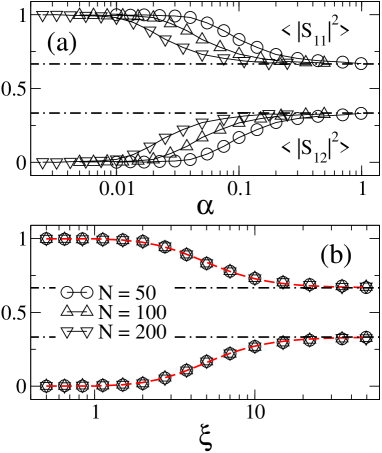
Figure 2: (Color online) Average $S$-matrix elements $\left\langle|S_{11}|^{2}\right\rangle$ and $\left\langle|S_{12}|^{2}\right\rangle$ for tight-binding random networks having $N$ nodes as a function of (a) $\alpha$ and (b) $\xi$, for $M=1$. The dot-dashed lines correspond to 2/3 and 1/3; the RMT prediction for $\left\langle|S_{11}|^{2}\right\rangle$ and $\left\langle|S_{12}|^{2}\right\rangle$, respectively, given by Eq. (5). Red dashed lines in (b) are Eqs. (16) and (17) with $\delta\approx 0.198$. Error bars in this and the following figures are not shown since they are much smaller than symbol size.

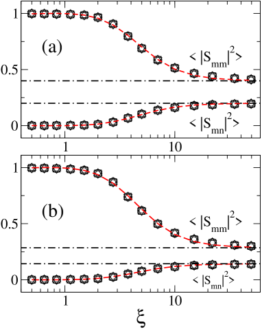
Figure 3: (Color online) Average $S$-matrix elements $\left\langle|S_{mm}|^{2}\right\rangle$ [with $mm=11$, 22, 33, and 44] and $\left\langle|S_{mn}|^{2}\right\rangle$ [with $mn=12$, 23, 34, and 41] for tight-binding random networks having $N=200$ nodes as a function of $\xi$ for (a) $M=2$ and (b) $M=3$. The dot-dashed lines correspond to the RMT prediction for $\left\langle|S_{mm}|^{2}\right\rangle$ and $\left\langle|S_{mn}|^{2}\right\rangle$; see Eq. (5). Red dashed lines are Eqs. (18) and (19) with (a) $\delta\approx 0.237$ and (b) $\delta\approx 0.242$.

Moreover, we have found that the universal behavior of $\left\langle|S_{11}|^{2}\right\rangle$ and $\left\langle|S_{12}|^{2}\right\rangle$, as a function of $\xi$, is well described by

$$\left\langle|S_{11}|^{2}\right\rangle = 1-\left\langle|S_{12}|^{2}\right\rangle\ ,$$ (16)

$$\left\langle|S_{12}|^{2}\right\rangle = \frac{1}{3}\left[\frac{1}{1+(\delta\xi)^{-2}}\right]\ ,$$ (17)

where $\delta$ is a fitting parameter. Eq. (16) is a consequence of the unitarity of the scattering matrix, $SS^{\dagger}=\mathbf{1}$, while the factor 1/3 in Eq. (17) comes from Eq. (5) with $M=1$. In Fig. 2(b) we also include Eqs. (16) and (17) (red dashed lines) and observe that they reproduce very well the corresponding numerical results. In fact, we have to add that Eqs. (16) and (17) also work well for other random matrix models showing a metal-insulator phase transition AMV09 .

For $M>1$ we observe the same scenario as for $M=1$: All $S$-matrix elements suffer a localization-delocalization transition as a function of $\xi$. See Fig. 3 where we plot some of the average $S$-matrix elements for $M=2$ and 3. Moreover, we were able to generalize Eqs. (16) and (17) to any $M$ as

$$\left\langle|S_{mm}|^{2}\right\rangle = 1-(2M-1)\left\langle|S_{mn}|^{2}\right\rangle\ ,$$ (18)

$$\left\langle|S_{mn}|^{2}\right\rangle = \left\langle|S_{mn}|^{2}\right\rangle_{\mbox{\tiny COE}}\left[\frac{1}{1+(\delta\xi)^{-2}}\right]\ .$$ (19)

Then, in Fig. 3 we also plot Eqs. (18) and (19) and observe very good correspondence with the numerical data. We also note that the fitting parameter $\delta$ slightly depends on $M$.

Finally we want to remark that concerning $\left\langle|S_{mn}|^{2}\right\rangle$, the RMT limit, expected for $\alpha\to 1$ or $\xi\to N$, is already recovered for $\xi\geq 30$.

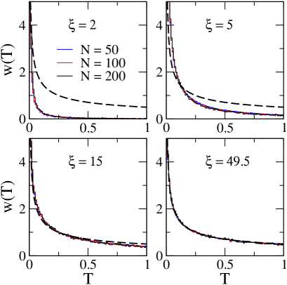
Figure 4: (Color online) Conductance probability distribution $w(T)$ for tight-binding random networks having $N$ nodes, in the case $M=1$, for some values of $\xi$. Dashed lines are $w(T)_{\mbox{\tiny COE}}$; the RMT prediction for $w(T)$ given by Eq. (6).

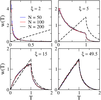
Figure 5: (Color online) Conductance probability distribution $w(T)$ for tight-binding random networks having $N$ nodes, in the case $M=2$, for some values of $\xi$. Dashed lines are $w(T)_{\mbox{\tiny COE}}$; the RMT prediction for $w(T)$ given by Eq. (7).

III.2 Conductance and shot noise power

Now we turn to the conductance statistics. In Figs. 4 and 5 we present conductance probability distributions $w(T)$ for $M=1$ and $M=2$, respectively. In both cases we include the corresponding RMT predictions. We report histograms for four values of $\xi$ and three network sizes. From these figures, it is clear that $w(T)$ is invariant once $\xi$ is fixed; i.e., once $\xi$ is set to a given value, $w(T)$ does not depend on the size of the network. We also recall that in the limit $\alpha\to 1$, $w(T)$ is expected to approach the RMT predictions of Eqs. (6) and (7). However, we observe that $w(T)$ is already well described by $w(T)_{\mbox{\tiny COE}}$ once $\xi\geq 30$. We observe an equivalent scenario for $w(T)$ when $M>2$ (not shown here).

We now increase further the number of attached leads. Then, in Figs. 6(a) and 7(a) we plot the average conductance $\left\langle T\right\rangle$ and the shot noise power $P$ for tight-binding random networks having $N=200$ nodes, for several values of $\xi$ with $M\in[1,5]$ (we recall that for $M=5$, ten single-channel leads are attached to the networks). It is clear from these plots that changing $\xi$ from small ($\xi<1$) to large ($\xi\gg 1$) values produces a transition from localized to delocalized behavior in the scattering properties of random notworks. That is, (i) for $\xi<0.5$, $\left\langle T\right\rangle\approx 0$ and $P\approx 0$; and (ii) for $\xi\geq 30$, $\left\langle T\right\rangle$ and $P$ are well given by the corresponding RMT predictions given by Eqs. (8) and (9), respectively. Equivalent plots are obtained (not shown here) for other network sizes.

Moreover, we have observed that $\left\langle T\right\rangle$ and $P$ as a function of $\xi$ behave (for all $M$) as $\left\langle|S_{mn}|^{2}\right\rangle$ does. I.e., they show a universal behavior as a function of $\delta\xi$ that can be well described by

$$X(\xi)=X_{\mbox{\tiny COE}}\left[\frac{1}{1+(\delta\xi)^{-2}}\right]\ ,$$ (20)

where $X$ represents $\left\langle T\right\rangle$ or $P$ and $\delta$ is the fitting parameter. Then, in Figs. 6(b) and 7(b) we plot $\left\langle T\right\rangle$ and $P$ normalized to their respective COE average values, as a function of $\delta\xi$ for $M\in[1,5]$. Notice that all curves for different $M$ fall on top of the universal curve given by Eq. (20).

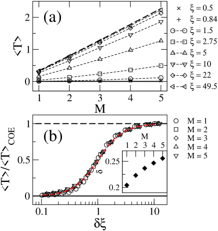
Figure 6: (Color online) (a) Average conductance $\left\langle T\right\rangle$ as a function of $M$ for tight-binding random networks having $N=200$ nodes for several values of $\xi$. (b) $\left\langle T\right\rangle/\left\langle T\right\rangle_{\mbox{\tiny COE}}$ as a function of $\delta\xi$ for $M\in[1,5]$. Insert: $\delta$ versus $M$. $\delta$ is obtained from the fitting of Eq. (20) to the $\left\langle T\right\rangle$ vs. $\xi$ data. Thick full lines correspond to $\left\langle T\right\rangle=0$. Dashed lines are (a) the RMT prediction for $\left\langle T\right\rangle$, given by Eq. (8); and (b) one. The red dashed line in (b) on top of the data is Eq. (20).

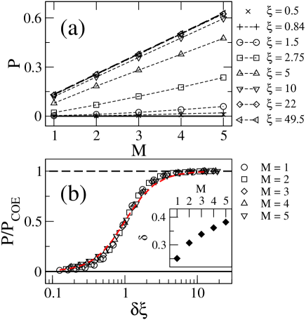
Figure 7: (Color online) (a) Shot noise power $P$ as a function of $M$ for tight-binding random networks having $N=200$ nodes for several values of $\xi$. (b) $P/P_{\mbox{\tiny COE}}$ as a function of $\delta\xi$ for $M\in[1,5]$. Insert: $\delta$ versus $M$. $\delta$ is obtained from the fitting of Eq. (20) to the $P$ vs. $\xi$ data. Thick full lines correspond to $P=0$. Dashed lines are (a) the RMT prediction for $P$, given by Eq. (9); and (b) one. The red dashed line in (b) on top of the data is Eq. (20).

III.3 Enhancement factor

Finally, in Fig. 8 we plot the elastic enhancement factor $F$ as a function of $\xi$ for random networks with $N=50$ nodes for $M=1$, 2, and 4. From this figure we observe that, for any $M$ (and also for any $N$, not shown here), $F$ decreases as a function of $\xi$ and approaches smoothly, for large $\xi$ ($\xi\to N$), the RMT limit value of $F_{\mbox{\tiny COE}}=2$. Also note that when $\xi\ll 1$, $F\propto\xi^{-2}$; which seems to be a signature of our random network model.

Figure 8: (Color online) Elastic enhancement factor $F$ as a function of $\xi$ for tight-binding random networks having $N=50$ nodes for $M=1$, 2, and 4. Black full line is Eq. (21) with $M=1$ and $\delta=0.198$. Red dashed lines are fittings of Eq. (22) to the data with $C=205$, 138, and 106 for $M=1$, 2 and 4, respectively. The horizontal black dashed line corresponds to the RMT limit value of $F_{\mbox{\tiny COE}}=2$.

To have an analytic support for the observations made above, we substitute Eqs. (18) and (19) into Eq. (10) to get the following estimation for $F$:

$$F\approx(2M+1)(\delta\xi)^{-2}+2\ .$$ (21)

Notice that Eq. (21) reproduces properly the behavior of $F$ for small and large $\xi$: $F\propto\xi^{-2}$ and $F\to 2$, respectively. Unfortunately, Eq. (21) does not describe qualitatively the curves of Fig. 8, see as example the black full line in this figure that corresponds to Eq. (21) with $M=1$. The reason of this discrepancy, as a detailed analysis shows, is that Eq. (19) overestimates the magnitude of $\left\langle|S_{mn}|^{2}\right\rangle$ when $\xi\ll 1$ and as a consequence Eq. (21) underestimates the magnitude of $F$ for those $\xi$-values. Then, to fix this issue we propose the following expression

$$F\approx C\xi^{-2}+2\ ,$$ (22)

where $C$ is a fitting constant, to describe the curves $F$ vs. $\xi$. In Fig. 8 we also show that Eq. (22) fits reasonably well the numerical data.

IV Conclusions

We study scattering and transport properties of tight-binding random networks characterized by the number of nodes $N$ and the average connectivity $\alpha$.

We observed a smooth crossover from localized to delocalized behavior in the scattering and transport properties of the random network model by varying $\alpha$ from small ($\alpha\to 0$) to large ($\alpha\to 1$) values. We show that all the scattering and transport quantities studied here are independent of $N$ once $\xi=\alpha N$ is fixed. Moreover, we proposes a heuristic and universal relation between the average scattering matrix elements $\left\langle|S_{mn}|^{2}\right\rangle$, the average conductance $\left\langle T\right\rangle$, and the shot noise power $P$ and the disorder parameter $\xi$. See Eq. (20). As a consequence, we observed that the onset of the transition takes place at $\delta\xi\approx 0.1$; i.e., for $\delta\xi<0.1$ the networks are in the insulating regime. While the onset of the Random Matrix Theory limit is located at $\delta\xi\approx 10$; that is, for $\delta\xi>10$ the networks are in the metallic regime. Also, the metal-insulator transition point is clearly located at $\delta\xi\approx 1$; see red dashed curves in Figs. 6(b) and 7(b). Here, $\delta\in[0.2,0.4]$ is a parameter that slightly depends on the number of attached leads to the network but also on the quantity under study, see inserts of Figs. 6(b) and 7(b).

Since our random network model is represented by an ensemble of sparse real symmetric random Hamiltonian matrices, in addition to random graphs of the Erdős-Rényi–type and complex networks, we expect our results to be also applicable to physical systems characterized by sparse Hamiltonian matrices, such as quantum chaotic and many-body systems.

- (1) A. L. Barabasi and R. Albert, Science 286, 509 (1999).
- (2) S. H. Strogatz, Nature 410, 268 (2001).
- (3) R. Albert and A. L. Barabasi, Rev. Mod. Phys. 74, 47 (2002).
- (4) A. L. Barabasi, Phil. Trans. R. Soc. A 371:20120375 (2013).
- (5) B. Derrida and G. J. Rodgers, J. Phys. A: Math. Gen. 26, L457 (1993).
- (6) C. P. Zhu and S. J. Xiong, Phys. Rev. E 62, 14780 (2000); Phys. Rev. B 63, 193405 (2001).
- (7) K. I. Goh, B. Klang, and D. Kim, Phys. Rev. E 64, 051903 (2001); G. J. Rodgers, K. Austin, B. Kahng, and D. Kim, J. Phys. A: Math. Gen. 38, 9431 (2005); T. Nagao and G. J. Rodgers, ibid 41, 265002 (2008).
- (8) O. Giraud, B. Georgeot, and D. L. Shepelyansky, Phys. Rev. E 72, 036203 (2005); 80, 026107 (2009); B. Georgeot, O. Giraud, and D. L. Shepelyansky, 81, 056109 (2010).
- (9) M. Sade, T. Kalisky, S. Havlin, and Berkovits, Phys. Rev. E 72, 066123 (2005); R. F. S. Andrade and J. G. V. Miranda, Physica A 356, 1 (2005); C. Kamp and K. Christensen, Phys. Rev. E 71, 041911 (2005); F. Slanina, Eur. Phys. J. B 85, 361 (2012).
- (10) J. N. Bandyopadhyay and S. Jalan, Phys. Rev. E 76, 026109 (2007); S. Jalan and J. N. Bandyopadhyay, Phys. Rev. E 76, 046107 (2007); Physica A 387, 667 (2008).
- (11) S. Jalan and J. N. Bandyopadhyay, Europhys. Lett. 87, 48010 (2009); S. Jalan, ibid 80, 046101 (2009); J. X. deCarvalho, S. Jalan, and M. S. Hussein, ibid 79, 056222 (2009); S. Jalan, N. Solymosi, G. Vattay, and B. Li, ibid 81, 046118 (2010); S. Jalan, G. Zhu, and B. Li, ibid 84, 046107 (2011).
- (12) G. Zhu, H. Yang, C. Yin, and B. Li, ibid 77, 066113 (2008);
- (13) L. Gong and P. Tong, ibid 74, 056103 (2006); A. L. Cardoso, R. F. S. Andrade, and A. M. C. Souza, Phys. Rev. B 78, 214202 (2008); L. Jahnke, J. W. Kentelhardt, R. Berkovits, and S. Havlin, Phys. Rev. Lett. 101, 175702 (2008).
- (14) I. Farkas, I. Derényi, H. Jeong, Z. Néda, Z. N. Oltvai, E. Ravasz, A. Schubert, A. L. Barabási, and T. Vicsek, Physica A 314, 25 (2002).
- (15) S. N. Dorogovtsev, A. V. Goltsev, J. F. F. Mendes, and A. N. Samukhin, Phys. Rev. E 68, 046109 (2003); Physica A 338, 76 (2004).
- (16) G. Ergün and R. Kühn, J. Phys. A: Math. Theor. 42, 395001 (2009); R. Kühn and J. vanMourik, ibid, 44, 165205 (2011).
- (17) O. Hul and L. Sirko, Phys. Rev. E 83, 066204 (2011).
- (18) A. Alcazar-Lopez, A. J. Martinez-Mendoza, and J. A. Mendez-Bermudez, unpublished.
- (19) G. Rodgers and A. J. Bray, Phys. Rev. B 37, 3557 (1988).
- (20) G. Rodgers and C. deDominicis, J. Phys. A: Math. Gen. 23, 1567 (1990); A. Khorunzhy and G. J. Rodgers, J. Math. Phys. 38, 3300 (1997).
- (21) Y. V. Fyodorov and A. D. Mirlin, J. Phys. A: Math. Gen. 24, 2219 (1991); Phys. Rev. Lett. 67, 2049 (1991); A. D. Mirlin and Y. V. Fyodorov, ibid 24, 2273 (1991).
- (22) S. N. Evangelou and E. N. Economou, Phys. Rev. Lett. 68, 361 (1992); S. N. Evangelou, J. Stat. Phys. 69, 361 (1992).
- (23) A. D. Jackson, C. Mejia-Monasterio, T. Rupp, M. Saltzer, and T. Wilke, Nucl. Phys. A 687, 405 (2001).
- (24) O. Mülken, V. Pernice, and A. Blumen, Phys. Rev. E 76, 051125 (2007).
- (25) O. Mülken and A. Blumen, Phys. Rep. 502, 37 (2011); A. Anishchenko, A. Blumen, and O. Mülken, Quantum Inf. Processing 11, 1273 (2012).
- (26) X. P. Xu, W. Li, and F. Liu, Phys. Rev. E 78, 052103 (2008). X. P. Xu and F. Liu, Phys. Lett. A 372, 6727 (2008); New J. Phys. 10, 123012 (2008); P. Li, Z. Zhang, X. P. Xu, and Y. Wu, J. Phys. A: Math. Theo. 44, 445001 (2011).
- (27) S. Salimi, R. Rradgohar, and M. M. Soltanzadeh, Intl. J. Quantum Inf. 08, 1323 (2010); E. Agliari, Physica A 390, 1853 (2011); F. Perakis and G. P. Tsironis, Phys. Lett. A 375, 676 (2011).
- (28) Z. Pluhar and H. A. Weidenmüler, Phys. Rev. Lett. 110, 034101 (2013).
- (29) P. A. Mello and N. Kumar, Quantum Transport in Mesoscopic Systems (Oxford University Press, Oxford, 2004).
- (30) P. Erdős and A. Rényi, Publ. Math. (Debrecen) 6, 290 (1959).
- (31) We remark that in the original Erdős-Rényi random graph model the on-site potentials are set to zero while the hopping integrals are all equal to one.
- (32) H. Schanz and T. Kottos, Phys. Rev. Lett. 90, 234101 (2003).
- (33) S. Gnutzmann, H. Schanz, and U. Smilansky, Phys. Rev. Lett. 110, 094101 (2013).
- (34) P. W. Anderson, Phys. Rev. 109, 1492 (1958).
- (35) B. I. Shklovskii, B. Shapiro, B. R. Sears, P. Lambrianides, and H. B. Shore, Phys. Rev. B 47, 11487 (1993).
- (36) B. L. Altshuler, V. E. Kravtsov, and I. V. Lerner, in Mesoscopic Phenomena in Solids, edited by B. L. Altshuler, P. A. Lee, and R. A. Webb (North-Holland, Amsterdam, 1991); Mesoscopic Quantum Physics, Proceedings of the Les Houches Session LXI, edited by E. Akkermans, G. Montambaux, J.-L. Pichard, and J. Zinn-Justin (North-Holland, Amsterdam, 1995); K. B. Efetov, Supersymmetry in Disorder and Chaos (Cambridge University Press, Cambridge, 1997).
- (37) T. Kottos and U. Smilansky, Phys. Rev. Lett. 79, 4794 (1997); Ann. Phys. (N.Y.) 273, 1 (1999); S. Gnutzmann and A. Altland, Phys. Rev. Lett. 93, 194101 (2004); Phys. Rev. E 72, 056215 (2005). S. Gnutzmann and U. Smilansky, Adv. Phys. 55, 527 (2006).
- (38) T. Kottos and H. Schanz, Physica E 9, 523 (2001).
- (39) T. Kottos and U. Smilansky, Phys. Rev. Lett. 85, 968 (2000); J. Phys. A 36, 3501 (2003).
- (40) O. Hul, S. Bauch, P. Pakonski, N. Savytskyy, K. Zyczkowski, and L. Sirko, Phys. Rev. E 69, 056205 (2004); M. Lawniczak, O. Hul, S. Bauch, P. Seba, and L. Sirko, idem 77, 056210 (2008); M. Lawniczak, S. Bauch, O. Hul, and L. Sirko, idem 81, 046204 (2010).
- (41) C. Mahaux and H. A Weidenmüller, Shell Model Approach in Nuclear Reactions, (North-Holland, Amsterdam,1969); J. J. M. Verbaarschot, H. A. Weidenmüller, and M. R. Zirnbauer, Phys. Rep. 129, 367 (1985); I. Rotter, Rep. Prog. Phys. 54, 635 (1991).
- (42) R. Landauer, IBM J. Res. Dev. 1, 223 (1957); 32, 336 (1988); M. Buttiker, Phys. Rev. Lett. 57, 1761 (1986); IBM J. Res. Dev. 32, 317 (1988).
- (43) E. N. Bulgakov, V. A. Gopar, P. A. Mello, and I. Rotter, Phys. Rev. B 73, 155302 (2006); D. V. Savin and H.-J. Sommers, idem 73, 081307(R) (2006); S. Heusler, S. Muller, P. Braun, and F. Haake, Phys. Rev. Lett. 96, 066804 (2006); J. Phys. A: Math. Gen. 39, L159 (2006).
- (44) H. L. Harney, A. Richter, and H. A. Weidenmüller, Rev. Mod. Phys. 58, 607 (1986); A. Muller and H. L. Harney, Phys. Rev. C 33, 1228 (1987).
- (45) J. A. Méndez-Bermúdez, V. A. Gopar, and I. Varga, Ann. Phys. (Berlin) 18, 891 (2009).
- (46) A. Alcazar-López, J. A. Méndez-Bermúdez, and I. Varga, Ann. Phys. (Berlin) 18, 896 (2009); J. A. Méndez-Bermúdez, V. A. Gopar, and I. Varga, Phys. Rev. E 82, 125106 (2010).