Dynamical symmetry approach and topological field theory for path integrals of quantum spin systems

Abstract

We develop a dynamical symmetry approach to path integrals for general interacting quantum spin systems. The time-ordered exponential obtained after the Hubbard-Stratonovich transformation can be disentangled into the product of a finite number of the usual exponentials. This procedure leads to a set of stochastic differential equations on the group manifold, which can be further formulated in terms of the supersymmetric effective action. This action has the form of the Witten topological field theory in the continuum limit. As a consequence, we show how it can be used to obtain the exact results for a specific quantum many-body system which can be otherwise solved only by the Bethe ansatz. To our knowledge this represents the first example of a many-body system treated exactly using the path integral formulation. Moreover, our method can deal with time-dependent parameters, which we demonstrate explicitly.

I Introduction

The path integral approach to strongly-correlated systems is a powerful method from many perspectives. In particular, it easily accounts for the topologically nontrivial terms in the action and it is a convenient starting point for various numerical schemes. Moreover, it allows to treat the correlated systems by a number of approximate analytical techniques, including the saddle point method, instanton analysis, and various perturbative expansions ref:Kleinert ; ref:Negele ; ZJ . On the other hand, only a limited number of path integrals are accessible to an exact evaluation, and to our knowledge there are no examples that could explicitly treat any nontrivial Bethe ansatz-solvable model. For spin systems the conventional method consists of inserting the resolution of identity on the space of the spin coherent states at every discretized time slice ref:Fradkin . Then the overlaps between different coherent states taken at consecutive time slices $\langle\zeta(t)|\zeta(t+\epsilon)\rangle$, where $\epsilon$ is the discretization time step, is approximated using the Taylor expansion in $\epsilon$. The important assumption behind this is the differentiability of the path $\zeta(t)$. This approximation eventually prohibits exact evaluation of the path integral.

Here we introduce a novel representation of lattice spin models, which does not rely on the spin coherent state representation, and which reveals a hidden dynamical (super)-symmetry structure. After performing the Hubbard-Stratonovich transform, the partition function or the evolution operator of a spin system quadratic in spin variables can be represented as an average of a time-ordered exponential. Based on the well known facts of the group theory, we represent the time-ordered exponential as a product of usual exponentials. However, the arguments of the disentangled exponentials are related to the original fields via a set of nonlinear differential equations. These equations can be interpreted as stochastic differential equations. The Hubbard-Stratonovich fields play the role of a noise, whose correlators are defined by the interaction matrix of the ordinal quantum spin system. Stochastic trajectories are non-differentiable in general and our approach takes this into account exactly and allows to derive results that can be obtained otherwise only using the Bethe ansatz. We show this explicitly on a non-trivial example rooted in quantum optics  ref:YudsonPRA . Moreover the stochastic interpretation suggests that there is a hidden supersymmetry, which eventually leads us to the formulation of the partition function of the quantum spin system as a correlation function of non-topological operators in the theory whose action is given by the topological field theory of Witten Witten ; FLN .

Sections 2 and 3 of this paper discuss the general aspects of our approach, while Section 4 illustrates the method on a non-trivial example of a many-body system. We compare our results to the Bethe ansatz solution within the limit of its applicability, and we also provide some explicit results beyond. This example provides a hint of utility of our approach for a larger class of spin systems. The Appendix contains a number of formulas, useful for analytical and numerical considerations.

II Disentanglement of the time-ordered exponential

We consider a generic interacting quantum spin model on a lattice,

$$H=\sum_{i,j}\Omega_{ij}^{ab}S_{i}^{a}S_{j}^{b}+\sum_{j}h^{a}_{j}S^{a}_{j}$$ (1)

where the lattice spin operators $S^{a}_{j}$ ($j$ being the lattice index) satisfy the commutation relations of the Lie algebra $g$, $[S^{a}_{i},S^{b}_{j}]=f^{ab}_{c}S^{c}_{j}\delta_{ij}$. The indices $a,b,c$ run from $1$ to $N$, where $N$ is the dimension of $g$, and $f^{ab}_{c}$ are the structure constants. Interactions between the spins are determined by the interaction matrix $\Omega^{ab}_{ij}$, which can be in general non diagonal in $a,b$ indices. We assume no particular restriction on the compactness of the corresponding Lie group $G$ while we assume that certain particular representation is chosen for the concrete physical problem (such as the spin-1/2 or spin-1 representations for the case of $g$ being $SU(2)$). We are interested in correlation functions of the model defined by Eq. (1), which is why we introduce the source terms $\mathcal{J}_{j}^{a}(t)$ and consider the generating functional

$$W[{\cal J}]=\operatorname{Tr}\exp\left(itH+i\sum_{j}\int{\cal J}^{a}_{j}(t)S^{a}_{j}\right).$$ (2)

The approach under discussion may work also in a more general setting, in which the matrix $\Omega^{ab}$ and the fields $h^{a}$ are assumed to be time-dependent functions. Moreover, it is straightforward to replace the trace in Eq. (2) by expectation values in certain $\left|\mathrm{in}\right\rangle$ and $\left|\mathrm{out}\right\rangle$. These generalize the approach to non-equilibrium evolution problems. For the equilibrium considerations one can perform the Wick rotation $it\rightarrow-\beta$.

Applying the Suzuki-Trotter discretization ref:Negele and introducing the Hubbard-Stratonovich transformation ref:HSTransform , we rewrite Eq. (2) into the following form (in the following repeated indices are assumed to be summed over)

$$W[{\cal J}]=\int D\mu(\phi)\prod_{j}{\cal T}_{c}\exp(i\int^{t}dt\Phi^{a}_{j}S^{a}_{j}),$$ (3)

where $D\mu(\phi)=\exp(-\sum_{jk}\phi^{a}_{k}(\Omega^{-1})^{ab}_{kj}\phi_{j}^{b})\prod_{j}D\phi^{a}$ is the Gaussian integration measure, $\Phi^{a}_{j}(t)=\phi^{a}_{j}(t)+h^{a}_{j}+{\cal J}^{a}_{j}(t)$, $\Omega^{-1}$ is a matrix inverse to $\Omega$, and ${\cal T}_{c}\exp$ denotes the time-ordered exponential. The index $c$ indicates a possible Keldysh contour ordering.

The main conceptual step of our approach is the following: the ”effective Hamiltonian” $\int dt\Phi^{a}_{j}(t)S_{j}^{a}$ at given $j$ is a linear combination of generators of $g$ and therefore its exponential is an element of the group $G$. The ${\cal T}$-ordered exponential is a directed product of ordinary exponentials, and hence a composition of elements of the Lie group. Any composition of elements of the Lie group $G$ is a certain element of $G$ itself. As such, this element can be written as a single exponential again. This generic mathematical fact defines the essence of our approach and exhibits a concept of dynamical symmetry: A Hamiltonian of the form of a linear combination of generators of the Lie algebra (with possibly time-dependent coefficients) has this Lie algebra as the spectrum-generating algebra Perelomov . We call the procedure of going from the time-ordered exponential to the product of the ordinary exponentials a disentanglement transformation. Similar philosophy has been recently used in ref:Kolokolov1 ; ref:Kolokolov2 ; ref:Kolokolov3 ; ref:Kolokolov4 ; ref:Kolokolov5Review ; ref:Kolokolov6 ; Galitski ; ref:Gefen1 ; ref:Gefen2 ; Chalker ; RPG .

It is clear that the original variables $\Phi^{a}(t)$ and a set of variables, which carries out a disentanglement are related in a non-trivial way. The easiest way to elucidate this relationship is to consider the definition of the ${\cal T}$-ordered exponential, namely $i\dot{U}(t)=\Phi^{a}(t)S^{a}U$. Since $U\in G$ and there is an inverse, $U^{-1}$ we write it as $i\dot{U}U^{-1}=\Phi^{a}(t)S^{a}$. The left-hand side of this equation is a current $J_{0}$ on the group, used e.g. for formulating the non-linear sigma models. Group manifold can be parametrized in a number of ways by a set of parameters $\{n^{a}\}$, ($a=1\ldots\dim G$). However, there is an important object — the Maurer-Cartan (MC) 1-form on $G$ — that allows us to write the underlying equations in a covariant way. Defining a right 1-form $R^{a}_{\alpha}$ via $i\dot{U}U^{-1}=i\partial_{\alpha}UU^{-1}\dot{n}^{\alpha}=iR^{a}_{\alpha}(\{n\})S_{a}\dot{n}^{\alpha}$, where $n^{\alpha}$ is a parametrization of a group, we arrive at a set of equations defining a relation between $\Phi^{a}(t)$ and a disentangling variables,

$$iR^{a}_{\alpha}(\{n\})\dot{n}^{\alpha}(t)=\Phi^{a}(t).$$ (4)

For a given parametrization $\{n\}$, the MC forms satisfy the MC equations, $\partial_{\alpha}R^{a}_{\beta}-\partial_{\beta}R^{a}_{\alpha}+f^{a}_{bc}R^{b}_{\alpha}R^{c}_{\beta}=0$, which are the defining equations for $R^{b}_{\alpha}$. Here and in Eq.(4) we for generality distinguish the upper and lower indexes, which are manipulated with the Killing-Cartan metrics $g_{\alpha\beta}=R^{a}_{\alpha}R^{b}_{\beta}\operatorname{Tr}(S^{a}S^{b})$. The equations (4) can in principle be resolved in terms on $\{\dot{n}^{a}\}$, however this can not be done globally if the topology of $G$ is non-trivial (e.g. for the $SU(2)$ case the sphere can not be covered by a single map). Also note that for $G$ interpreted as the Riemann manifold, MC forms are proportional to vielbeins (tetrads) $e^{a}_{\beta}$.

We envision at least two general ways to proceed. First, thanks to the Gaussian measure $D\mu(\phi)$ of the Hubbard-Stratanovich fields we can interpret Eqs. (4) as a set of stochastic differential equations on the group manifold. Second, one can use Eqs. (4) as defining rules for the change of variables in the path integral (3), to go from variables $\Phi^{a}$ to the new variables $n^{a}$ that define a disentanglement transform. Here we elaborate more on the first approach.

For a concrete implementation of this approach we consider first the case of $g=su(2)$ and come back to a generic discussion later on. As we have said, many different parametrizations for a group element $U$ are possible. These include the Euler angle parametrization, $U_{E}(\alpha,\beta,\gamma)=\exp(i\alpha S^{3})\exp(i\beta S^{2})\exp(i\gamma S^{3})$, the covariant parametrization, $U_{C}({\bf A})=\exp(i{\bf A}\cdot{\bf S})$, and the Gauss parametrization which can be globally defined on the group manifold WN

$$U_{G}(\xi_{\pm},\xi_{z})=\exp(\xi_{+}S^{+})\exp(\xi_{z}S^{z})\exp(\xi_{-}S^{-}),$$ (5)

on which we mostly focus. For the latter parametrization we can derive the following set of equations (in imaginary time),

$$\Phi_{-} = \dot{\xi_{+}}-\xi_{+}\dot{\xi_{z}}-\xi_{+}^{2}e^{-\xi_{z}}\dot{\xi_{-}}$$

$$\Phi_{z} = \dot{\xi_{z}}+2\xi_{+}e^{-\xi_{z}}\dot{\xi_{-}}$$ (6)

$$\Phi_{+} = e^{-\xi_{z}}\dot{\xi_{-}}$$

and inversely,

$$\dot{\xi_{+}} = \Phi_{-}+\Phi_{z}\xi_{+}-\Phi_{+}\xi_{+}^{2},$$

$$\dot{\xi_{z}} = \Phi_{z}-2\Phi_{+}\xi_{+},$$ (7)

$$\dot{\xi_{-}} = \Phi_{+}\exp(\xi_{z}).$$

The initial conditions $\xi_{\pm,z}(0)=0$ follow from the relation $U(0)=1$. For the real time evolution the factor of $i$ should be present in front of $\dot{\xi}_{\pm,0}$.

The trace of the evolution operator can be easily computed for the spin-1/2 representation of the evolution operator, $\operatorname{Tr}U_{G}=2\cosh(\xi_{z}/2)+\xi_{+}\xi_{-}\exp(-\xi_{z}/2)$. For a generic representation of spin $s$ the covariant form $U_{C}$ yields a compact formula for the characters, $\chi^{s}(|{\bf A}|)=\sum_{m=-s}^{m=s}\exp(-im|{\bf A}|)=\sin\left[(s+\frac{1}{2})|{\bf A}|\right]/\sin\left[\frac{1}{2}|{\bf A}|\right]$, while for the $su(N)$ case one can use the celebrated Weyl determinant formula for the characters Lie-group ; KSK .

Next, by looking at the Eqs. (II) we realize that only the equation for $\xi_{+}$ is independent, while the solutions for $\xi_{z,-}$ can be obtained from the one for $\xi_{+}$. This motivates us to look for further change of variables. This can be done in different ways. In particular, by introducing new fields $\psi^{\pm,z}$ via the following correspondence $\xi_{+}=\psi^{-}$, $\xi_{z}=\int_{0}^{t}\psi^{z}(t^{\prime})dt^{\prime}$ and $\xi_{-}=\int_{0}^{t}\psi^{+}(t^{\prime})\exp(\int_{0}^{t^{\prime}}\psi^{z}(t^{\prime\prime})dt^{\prime\prime})dt^{\prime}$ we obtain $\Phi^{z}=\psi^{z}+2\psi^{+}\psi^{-}$, $\Phi^{+}=\psi^{+}$, and $\Phi^{-}=\dot{\psi}^{-}-\psi^{z}\psi^{-}-\psi^{+}(\psi^{-})^{2}$. This representation was found in ref:Kolokolov1 ; ref:Kolokolov2 ; ref:Kolokolov3 ; ref:Kolokolov4 ; ref:Kolokolov6 ; ref:Kolokolov5Review and more recently in ref:Gefen1 ; ref:Gefen2 . The measure of integration changes correspondingly, $D\phi^{z}D\phi^{+}D\phi^{-}={\cal M}D\psi^{z}\psi^{+}D\psi^{-}$, where ${\cal M}_{\psi}=c_{\psi}\exp(-\frac{1}{2}\int_{0}^{t}\psi^{z}(t))dt)$ is the Jacobian of the transformation. The constant $c_{\psi}$ fixes the normalization, and can be adjusted e.g. comparing to a non-interacting system. The following change of variables

$$\xi_{+} = \rho^{-},\qquad\xi_{z}=\int_{0}^{t}(\rho^{z}-\rho^{+}\rho^{-}),$$

$$\xi_{-} = \int_{0}^{t}\rho^{+}\exp\left[\int_{0}^{t}(\rho^{z}-\rho^{+}\rho^{-})\right],$$ (8)

leads to the following equations:

$$\Phi^{+} = \rho^{+},$$

$$\Phi^{-} = \dot{\rho}^{-}-\rho^{-}\rho^{z},$$

$$\Phi^{z} = \rho^{z}+\rho^{-}\rho^{+}.$$ (9)

The differential equation for $\dot{\rho}$ can be formally solved,

$$\rho^{-}(t) = \exp\left(\int_{0}^{t}\rho^{z}(t^{\prime})dt^{\prime}\right)$$

$$\times \int_{0}^{t}\exp\left(-\int_{0}^{t^{\prime}}\rho^{z}(t^{\prime\prime})dt^{\prime\prime}\right)\Phi^{-}(t^{\prime})dt^{\prime},$$

where we assumed the initial condition $\rho^{-}(0)=0$. Therefore in this representation we implicitly resolved the non-linearity of the equations in exchange for the non-locality in time. Variables $\xi_{\pm,z}$ can be now expressed exactly via $\rho^{z},\phi^{+},\phi^{-}$. Therefore we can use it to construct some mixture representation which involves $\phi$-variables and $\rho^{z}$ simultaneously. This representation suggests that the variable $R(t)=\int_{0}^{t}\rho^{z}(x)dx$ (such that $\dot{R}=\rho^{z}(t)$) considered as an independent variable might be useful. The Jacobian in this case reads ${\cal M}_{\rho}=c_{\rho}\exp(\frac{1}{2}\int_{0}^{t}(-\rho^{z}+\rho^{-}\rho^{+}))$. One more example is given the change of variables

$$\xi_{+} = \lambda^{-},$$

$$\xi_{z} = \int_{0}^{t}(\lambda^{z}-2\lambda^{+}\lambda^{-}),$$ (11)

$$\xi_{-} = \int_{0}^{t}\lambda^{+}\exp\left[\int_{0}^{t}(\lambda^{z}-2\lambda^{+}\lambda^{-})\right],$$

which leads to the following equations

$$\Phi^{+} = \lambda^{+},$$

$$\Phi^{-} = \dot{\lambda}^{-}-\lambda^{-}\lambda^{z}+(\lambda^{-})^{2}\lambda^{+},$$ (12)

$$\Phi^{z} = \lambda^{z}$$

The advantage of this representation lies in the simplicity of the relationship between the $+$ and $z$-components of the fields. This can be useful for some particular physical situations. Jacobian of the change of variables from $\phi^{\pm,z}$ to $\lambda^{\pm,z}$ is ${\cal M}_{\lambda}=c_{\lambda}\exp\left(\frac{1}{2}\int_{0}^{t}(-\lambda^{z}+2\lambda^{-}\lambda^{+})\right)$.

We note that there is an infinite number of other parametrizations, which could be constructed in a similar fashion. Based on the above parametrizations, one could conjecture that the determinant of the transformation in the Gauss decomposition can be expressed in the form of a group element corresponding to the time averaged Cartan subalgebra.

While in general the Riccati equations encountered above can not be solved analytically, we note that one can establish an interesting connection to the theory of the KdV (Korteweg-de Vries) equation ref:KDV . Namely, using the projective linear (Möbius) transformation, the Riccati equation can always be put into the in the form $iy^{\prime}(x)+y^{2}(x)=k^{2}-u(x)$ where $u(x)\equiv u({\bf\Phi}(x))$ is a known function of the HS variables ${\bf\Phi}(x)$, $x\equiv x(t)$ being a reparametrized time variable, and $k$ a real parameter (which could related to real physical parameters, e.g. magnetic field or $\hbar$ in the WKB series). The function $y(x)$ then admits a series expansion $y(x,k)=k+\sum_{n\geq 1}y_{n}(x)(2k)^{-n}$. Here, all even coefficients $y_{2n}$ are total derivatives and imaginary, while the first few nontrivial terms are $y_{1}=u(x)$, $y_{3}(x)=u^{2}$, $y_{5}=u^{3}+(u^{\prime})^{2}/2$, $y_{7}=5u^{4}/2-5u^{2}u^{\prime\prime}/2+(u^{\prime\prime})^{2}/2$, etc. The integrals $\int dxy_{2n+1}$ form the (Poisson) commuting integrals of the KdV equation. It would be interesting to understand the implications of this observation on our path-integral formulation below.

It can be shown that a generalization of the disentangling transformation for other groups — such as $SU(N)$ — is straightforward: The resulting set of equations will have the form of the matrix Riccati equation. On the other hand, a generalization for super-groups is more tricky and should be studied case by case, especially for atypical representations.

III Stochastic interpretation, supersymmetry and topological field theory formulation

The Hubbard-Stratonovich transformation introduces a Gaussian measure for the fluctuating fields $\phi^{a}_{j}$. This suggests that the differential equations for the disentangling variables $\xi_{\pm},x_{z}$ can be interpreted as a set of stochastic differential (generalized Langevin) equations. Generically, solutions of these equations are non-differentiable paths which should be treated carefully using the appropriate discretization prescriptions (see Appendix). This leads to the effective Lagrangian formulation (path integral) formulation and, on the other hand, reveals the hidden super-symmetry structure of the lattice spin systems. Here we establish the connection between our disentanglement procedure and the theory of stochastic differential equations.

III.1 Stochastic interpretation

Provided the MC form (vielbein) is invertible, the disentangling equations can be put into the form

$$i\dot{n}^{\alpha}_{j}=(R^{a}_{\alpha})^{-1}_{j}\Phi^{a}_{j}$$ (13)

for every lattice site $j$. The path integral formulation of the stochastic processes is a delicate issue and has a long history. The difficulty comes from the proper definition of the continuous-in-time effective Lagrangian from the discretized version of the stochastic processes. This issue was carefully elaborated upon in a series of earlier works LRT (and rediscovered recently in Arnold ) where it was shown that the result for the effective Lagrangian is a two-parametric family labeled by $r,s\in[0,1]$ which stand for discretization of the stochastic variable and the noise respectively. While the mid-point discretization $r=s=1/2$ corresponds to the Stratonovich convention, the $r=s=0$ is the Ito convention. It is convenient to introduce a multi-index $\mu=(a=1,2,3;j=1,\ldots N)$ and rewrite the Eq. (13) in the following form

$$i\dot{q}^{\mu}=-F^{\mu}({\bf q})+\sigma^{\nu}_{\mu}({\bf q})\tilde{\phi}^{\mu},$$ (14)

where $q^{\mu}=(n^{a})_{j}$, $F^{\mu}({\bf q})$ is a noise-free (deterministic part) of the equations (which collects the terms containing the magnetic field $h^{a}$ and the source term ${\cal J}(t)$, and $\sigma^{\mu}_{\nu}({\bf q})=(R^{a}_{\alpha})^{-1}_{k}O_{kj}$ is a matrix composed of MC forms $(R^{a}_{\alpha})_{j}$, and the transformation matrix $O_{kj}$, which puts the noise $\phi_{j}^{a}$ into the form of the Gaussian normalized white noise, $\langle\tilde{\phi}^{\mu}(t)\tilde{\phi}^{\nu}(t^{\prime})\rangle=\delta^{\mu\nu}\delta(t-t^{\prime})$. This can be always done as soon as the matrix $\Omega^{a,b}_{i,j}$ is non-degenerate. For our lattice spin system the components of the matrix $O_{jk}$ are therefore made of the Fourier coefficients normalized by the Fourier frequencies. The generalized vielbeins $\sigma^{\mu}_{\nu}$ normalized as $\sigma^{\mu}_{\rho}\sigma_{\mu\nu}=\delta_{\rho\nu}$ define the metric tensor $g_{\mu\nu}=\sigma_{\mu\rho}\sigma_{\nu\rho}$, so that $g^{\mu\nu}g_{\nu\rho}=\delta_{\nu\rho}$. The effective continuous-in-time Lagrangian then takes the following form

$${\cal L}_{r,s}[q,\dot{q}] = \frac{1}{2}g_{\mu\nu}(\dot{q}^{\mu}+F^{\mu}(q))(\dot{q}^{\nu}+F^{\nu}(q))$$ (15)

$$+ s\sigma_{\gamma\rho}\partial_{\nu}\sigma^{\nu}_{\rho}(\dot{q}^{\gamma}+F^{\gamma}(q))-r\partial_{\mu}F^{\mu}(q)$$

$$+ \frac{1}{2}s^{2}\partial_{\mu}\sigma^{\nu}_{\rho}\partial_{\nu}\sigma^{\mu}_{\rho}.$$

This general form of the Lagrangian can be simplified for particular physical systems. The integration measure in the path integral reads $D(q/\sqrt{\det{g_{\mu\nu}}})$. This representation is invariant with respect to the change of the particular representation and/or parametrization. The partition function or the time-evolution operator for the lattice spin system is than the expectation value of the operator $O_{N}=\prod_{j}U(q_{j})$, $W[{\cal J}]=\int D(q/\sqrt{\det{g_{\mu\nu}}})O_{N}\exp(-\int dt{\cal L}_{r,s}[q,\dot{q}])$.

III.2 Super-symmetry and connection to topological field theory

We come back to the general discussion of certain global properties of our approach. We would like to keep all stochastic trajectories without making any approximations. To do this we introduce an identity for every lattice point (a customary trick in field theory ZJ )

$$1=\int D[U]\det(M)\delta(J_{0}-\Phi),$$ (16)

where we introduced the matrix notations for $\Phi\equiv\Phi^{a}S_{a}$, the current $J_{0}=i\dot{U}U^{-1}$, and the Jacobian $M_{ab}=\delta J_{0}/\delta U_{ab}$ of the transformation. Here $d[U]$ is the Haar invariant integration measure on $G$, satisfying $\int d[U]f(U)=\int d[U]f(UV)$ for any trace-like function $f(U)$. Then $\delta(J_{0}-\Phi)=\int d\Lambda/(2\pi i)\exp[-Tr(\Lambda(J_{0}-\Phi)]$ (where the integration is performed along the imaginary axis) defines dual fields $\Lambda_{j}^{a}$, $\Lambda=\Lambda^{a}S_{a}$. Introducing the anti-commuting Faddev-Popov ghosts $C^{a},\bar{C}^{a}$ and using the Grassmann integration, one can write $\det M=\int d\bar{C}dC\exp(\bar{C}^{a}M_{ab}C^{b})$ to obtain an effective generating functional after integrating out the stochastic fields,

$$W[h] = \int d[U]d\Lambda d\bar{C}dC\exp(-\sum_{j}{\cal S}_{j})\prod_{j}\mbox{Tr}U_{j}$$ (17)

$${\cal S}_{j} = Tr[\Lambda(J_{0}-h)]_{j}-\bar{C}_{j}D_{0}C_{j}+Tr(\Lambda_{j}\Omega_{jk}\Lambda_{k}).$$

Here $D_{0}=\partial_{t}-J_{0}$ is the covariant derivative in time direction, $j$ is the lattice site index, and $C\equiv\{c^{a}\}$ represents a vector of Grassman variables. In this representation a generating functional looks like an expectation value of the Polyakov-like string $\prod_{j}\mbox{Tr}U_{j}$ for a theory described by the action $\sum_{j}S_{j}$. In principle, some of the variables in the effective action can be traced out explicitly. For instance, the variables $\Lambda$ enter quadratically and can be integrated out; the corresponding effective theory would look like the current-current interacting sigma-model coupled to fermions. The Grassmann part can be shown to lead to a finite contribution, which can be computed explicitly. This eventually produces the form (15) of the effective action since the Grassmann variables propagator $\langle\bar{C}(t)C(t)\rangle=s$ where the parameter $0\leq s\leq 1$ is the discretization introduced above. The group variables enter the action quadratically into and can be partially (because the expression for $U(n^{a})$ is not quadratic) integrated out. However at this point we would like to keep all the variables as well as their duals to demonstrate an underlying super-symmetry, which is difficult to see otherwise.

The hidden BRST super-symmetry BRST can be traced back to the stochastic nature of differential equations (4) or (II) on the Lie group manifold. In this sense it is a general feature of stochastic equations first noticed in PS ,FT (see also ZJ ). The super-symmetry transformation $\delta$ on variables in (III.2) is induced by

$$\delta\Lambda = 0,\qquad\delta\bar{C}=\epsilon\Lambda$$ (18)

$$\delta U = \epsilon UC,\qquad\delta C=-\epsilon C^{2},$$ (19)

and as a consequence, $\delta J_{0}=\epsilon D_{0}C$ and $\delta(D_{0}C)=0$. In components it reads $\delta c^{a}=-\frac{1}{2}f^{a}_{bc}\epsilon c^{b}c^{c}$. The action $\sum_{j}{\cal S}_{j}$ is therefore BRST exact, $\delta{\cal S}=0$. In terms of the group parameters $n^{a}$ the BRST charge can be represented by the action of the operator

$${\cal Q}=\sum_{j}(c^{a}\delta_{n^{a}}+\Lambda_{a}\delta_{\bar{c}^{a}})_{j},$$ (20)

so that ${\cal Q}^{2}=0$. Action on any functional is defined by $\{{\cal Q},X_{j}\}={\cal Q}X_{j}$. One can further show that

$${\cal S} = \{{\cal Q},V\}$$ (21)

$$V = \sum_{j}\bar{c}^{a}_{j}J_{0,j}^{a}+\sum_{i,j}\bar{c}^{a}_{i}\Omega_{ij}^{ab}\Lambda^{b}_{j}$$

$$= \sum_{j}\bar{c}^{a}_{j}J_{0,j}^{a}+\sum_{ij}\Omega_{ij}^{ab}\{Q,\bar{c}^{a}_{i}\{Q,\bar{c}^{b}_{j}\}\}.$$

In this form the action is in the form of the topological field theory of Witten Witten . It is easy to see that it is ${\cal Q}$-exact. The action of the ${\cal Q}$ operator on $U$ is non-zero, and therefore the lattice spin-system partition function is equivalent to computing expectation value of product of non-exact operators in this theory. Recently, progress in computing ”non-topological” (non-BPS) observables in topological field theories has been made in the framework of instantonic filed theory FLN . Concrete applications of these developments to the spin systems shall be discussed elsewhere. We emphasize that this representation of the interacting spin system is exact, since we kept all the non-differentiable path-integral trajectories exactly.

There are several possible implications of the SUSY/topological field theory structure. First, there are Ward-Takahashi identities associated with this super-symmetry. They lead to the fluctuation-dissipation theorem and work relations work-relation . Second, these identities allow to establish renormalization group prescriptions for the action. In particular we believe that one can establish the RG flow equations using the generalized tetrads $\sigma^{\mu}_{\nu}$ in the form of the geometric flow developed in Friedan . Third, there is a phenomenon of dimensional reduction PS-prl , coming from two additional Grassmann coordinates in the effective action. Application of these phenomena to spin systems could lead to an interesting relationships between spin systems defined in different dimensions. Fourth, a SUSY breaking pattern is rather restrictive. There are in general three scenarios: unbroken SUSY, breaking on the mean field level, and dynamical breaking. We believe that one may classify spin systems according to these scenarios. Fifth, the formulation in terms of the topological field theory could shed a new light on the origin of the topological order in certain spin systems. Moreover, one of the central concept of the topological theory, the Witten index, seems to have direct relevance to the sign problem Ovch .

IV Explicit demonstration of the method. Comparison with the Bethe ansatz and beyond

We shall illustrate the technique discussed in the previous sections by considering a problem of a single atom interacting with a one-dimensional photonic waveguide, treated within the Rotating Wave Approximation (RWA). This problem has been solved by the Bethe ansatz in ref:YudsonPRA , see also ref:BeforeYudson ; ref:ShiSunFan2 ; ref:ShiSunFan3 .

IV.1 The model and the observables

We assume that the photons in the waveguide feature a linear dispersion with two (left,right) branches, described by annihilation operators $a_{R,L}$. For one scatterer only, it is convenient to work in the basis of even/odd photons $a_{e,o}=(a_{R}\pm a_{L})/\sqrt{2}$. Odd photons $a_{o}$ do not interact with the atom, which is why they evolve trivially as free photons. The interacting part of the evolution is hidden in the even component $a_{e}$. From now on we focus purely on this nontrivial part and drop the index $e$ ($a_{e}\equiv a$). We consider the interaction between a collection of $M$ atoms, located within a region much smaller than the wavelength of light, and the even component of the photonic field. The atoms may be modeled as a single spin ${\hat{\mathrm{S}}}$ of magnitude $j=M/2$. The RWA Hamiltonian of the system then reads ref:BeforeYudson ; ref:YudsonPRA

$${\hat{\mathrm{H}}}=\sum_{k}k{a^{\dagger}_{k}}{a^{\vphantom{\dagger}}_{k}}+\Delta(t){\hat{\mathrm{S}}}^{z}+g(t)\sum_{k}\left({\hat{\mathrm{S}}}^{+}{a^{\vphantom{\dagger}}_{k}}+{\hat{\mathrm{S}}}^{-}{a^{\dagger}_{k}}\right)$$ (23)

We have assumed $k$-independent, but potentially time-dependent light-matter coupling $g(t)$, as well as time dependent atomic detuning $\Delta(t)$ (to save space, we in the following drop the explicit time dependence from them).

Many interesting physical properties of this mode may be expressed in terms of specific matrix elements of the evolution operator. For the sake of calculations, we add the auxiliary photonic sources $J^{(*)}_{k}(t)$, which serve the purpose of generating photons in the in- and out-states. They are set to zero at the end of the calculations. A generic matrix element of the evolution operator in presence of the photonic sources reads

$$\mathcal{U}_{oi}:=\left\langle\mathrm{out}\middle|\mathcal{T}\,e^{-i\int_{t_{1}}^{t_{2}}dtH+\sum_{k}\left(J^{*}_{k}(t){a^{\vphantom{\dagger}}_{k}}+J_{k}(t){a^{\dagger}_{k}}\right).}\middle|\mathrm{in}\right\rangle.$$ (24)

We require that both $\left|\mathrm{out}\right\rangle$ and $\left|\mathrm{in}\right\rangle$ are tensor products of vacuum state within the photonic subspace and a certain spin state. For instance, the amplitude of the decay of a fully excited state ($s^{z}=M/2$) into $2j$ photons can be related to Eq. (24) as

$$T_{k_{1},\dots,k_{2j}}:=\left\langle k_{1},\dots,k_{2j};-j\middle|\mathcal{U}(\infty,0)\middle|0;j\right\rangle=\\ \frac{\partial^{2j}}{\partial J^{*}_{k_{1}}\dots\partial J^{*}_{k_{2j}}}\left\langle-j\middle|\mathcal{T}\,e^{-i\int_{0}^{\infty}dtH}\middle|j\right\rangle.$$ (25)

Also the problem of finding the scattering matrix of $n$ photons scattering on the atoms can be reduced to Eq. (24) using the LSZ formalism ref:LSZ1 ; ref:ShiSunFan3 . This formalism expresses the $T$-matrices of the scattering

$$iT_{k_{i}\rightarrow p_{i}}=(2\pi)^{n}\times\\ G^{(2n)}(\{k_{i}\},\{p_{i}\})\prod_{s=1}^{n}\left(\mathcal{G}_{0}^{-1}(k_{s})\mathcal{G}_{0}^{-1}(p_{s})\right)|_{\mathrm{on-shell}}$$ (26)

via the $n$-particle Green function, calculated as

$$G^{(2n)}=\frac{(-1)^{n}\delta^{2n}\log Z[J,J^{*}]}{\delta J_{1}\ldots\delta J_{n}\delta J^{*}_{1}\ldots J^{*}_{n}},$$ (27)

where $Z[J,J^{*}]$ is the generating functional of the Green functions ref:Negele defined by the equation

$$Z[J,J^{*}]=\left\langle-j\middle|\mathcal{T}\,e^{-i\int_{-\infty}^{\infty}dtH+\sum_{k}\left(J^{*}_{k}(t){a^{\vphantom{\dagger}}_{k}}+J_{k}(t){a^{\dagger}_{k}}\right).}\middle|-j\right\rangle.$$ (28)

This obviously forms a special case of Eq. (24).

IV.2 Implementing disentangling transform and the stochastic formulation

We may treat the amplitude (24) within the path-integral approach. We rewrite the amplitude as a coherent state path integral over the photonic variables, while we retain the time-ordering for the spin variables ref:Negele

$$\mathcal{U}_{oi}=\int\mathcal{D}[a,a^{*}]\left\langle\mathrm{out}\right|\mathcal{T}\,e^{i\int dt\sum_{k}a^{*}_{k}(i\partial_{t}-k)a_{k}}\times\\ e^{i\int dt\left\{\sum_{k}\left[-g\left(a^{*}_{k}{\hat{\mathrm{S}}}^{-}+a_{k}{\hat{\mathrm{S}}}^{+}\right)+J^{*}_{k}a_{k}+J_{k}a_{k}^{*}\right]-\Delta{\hat{\mathrm{S}}}^{z}\right\}}\left|\mathrm{in}\right\rangle.$$ (29)

The integral over the bosonic degrees of freedom may be performed explicitly and gives rise to a spin model with an effective spin-spin interaction. Thanks to the linearity of the photonic spectrum, this spin-spin interaction happens to be local in time, which simplifies the calculations enormously. After some algebraic manipulations we arrive at the expression

$$\mathcal{U}_{oi}=\mathcal{U}^{0}_{oi}\left\langle\mathrm{out}\right|\mathcal{T}\,e^{\int dt-\frac{|g|^{2}}{2}{{\hat{\mathrm{\bm{S}}}}}^{2}}\times\\ e^{\int dt\left\{\frac{|g|^{2}}{2}{S^{z}}^{2}-\left[i\Delta+\frac{|g|^{2}}{2}\right]S^{z}+\mathcal{J}S^{+}+\mathcal{J}^{*}S^{-}\right\}}\left|\mathrm{in}\right\rangle,$$ (30)

with

$$\mathcal{J}^{\mp}(t):=g(t)\sum_{k}\int_{0}^{\infty}d\tau J_{k}^{(*)}(t\mp\tau)e^{-ik\tau}.$$ (31)

The symbol $\mathcal{U}^{0}_{oi}$ denotes the free-photonic-evolution part of the amplitude, which is irrelevant for the problems under consideration and consequently can be ignored. As explained in the first part of this paper, the natural way of decoupling the spin-spin interaction is via the Hubbard-Stratonovich transform (local in time) ref:HSTransform . The decoupling converts the exponent in Eq. (30) into a linear form, disentangleable using Eq. (5), at the expense of introducing a real-valued white-noise field $\Phi(t)$:

$$\mathcal{U}_{oi}=\mathcal{U}^{0}_{oi}\Big{\langle}\left\langle\mathrm{out}\right|\mathcal{T}\,e^{\int dt-\frac{|g|^{2}}{2}\bm{S}^{2}}\times\\ e^{\int dt\left\{\left[g\Phi-i\Delta-\frac{|g|^{2}}{2}\right]S^{z}+\mathcal{J}^{-}S^{+}+\mathcal{J}^{+}S^{-}\right\}}\left|\mathrm{in}\right\rangle\Big{\rangle}_{\Phi},$$ (32)

where we define the white-noise averaging $\langle\dots\rangle_{\Phi}$ to be

$$\langle\mathcal{A}[\Phi]\rangle_{\Phi}=\frac{\int\mathcal{D}[\Phi]e^{-\frac{1}{2}\int dt\Phi^{2}(t)}\mathcal{A}[\Phi]}{\int\mathcal{D}[\Phi]e^{-\frac{1}{2}\int dt\Phi^{2}(t)}}.$$ (33)

The evolution operator in Eq. (32) can be now readily disentangled using the technology explained in the first part of this paper. The evolution of the new variables $\xi_{\pm,z}$ is governed by a specific form of Eqs. (II), which we converted into the Ito form ref:Gardiner

$$\dot{\xi}_{+}=\mathcal{J}^{-}-i\Delta\xi_{+}-\mathcal{J}^{+}\xi_{+}^{2}+|g|\xi_{+}\Phi,$$ (34)

$$\dot{\xi}_{z}=-[i\Delta+{|g|^{2}/2}]-2\mathcal{J}^{+}\xi_{+}+|g|\Phi,\quad\dot{\xi}_{-}=\mathcal{J}^{+}e^{\xi_{z}}.$$

These equations form a set of non-linear stochastic differential equations (SDE) in the Ito form ref:Gardiner . Because of their nonlinearity, it is not possible to write down their explicit solution. We may, however, express the quantities of interest in terms of $\xi_{\pm,z}$ and write down the underlying SDE for these, utilizing the Ito lemma ref:Gardiner . Averaging these w.r.t. the noise $\Phi$ we get rid of the noise term and arrive at ordinary differential equations for the averages. Inspecting the matrix elements of Eq. (25) and Eq. (28) and comparing them to the disentangling transformation of Eqs. (II), we conclude that these are straightforwardly related to the $\Phi$-averages of the functions $\xi_{-}^{2j}e^{-j\xi_{z}}$, or $e^{-j\xi_{z}}$, respectively. The Ito lemma applied to these, however leads to unclosed equations, because extra powers of $\xi_{\pm}$ pop up. This obstacle may be overcome by considering a more general problem, in particular a hierarchy of equations for the functions $\xi_{+}^{n}e^{-j\xi_{z}}$, or $\xi_{-}^{n}e^{(j-n)\xi_{z}}$, respectively. This includes the desired quantities as a special case. Averaging these equations as indicated above, we obtain a closed set of ordinary differential equations for the following averages

$$F_{n}:=\left\langle\xi_{+}^{n}e^{-j\xi_{z}}\right\rangle_{\Phi},\quad R_{n}:=\left\langle\xi_{-}^{n}e^{(j-n)\xi_{z}}\right\rangle_{\Phi},$$ (35)

with $0\leq n\leq 2j$. The physically interesting quantities stem from $F_{0}$ and $R_{2j}$, respectively. These auxiliary quantities satisfy by definition the initial conditions $F_{0}(t_{1})=1$, $F_{n>0}(t_{1})=0$ (the same for $R_{n}$). Based on Eqs. (34) the quantities $F_{n}$ and $R_{n}$ satisfy a simple system of linear ordinary differential equations (the noise has been already averaged out!)

$$\dot{F_{n}}=\left[i\Delta\left(j-n\right)+\frac{g^{2}}{2}\left(j\left(j+1\right)-2jn+n(n-1)\right)\right]F_{n}\\ +n\mathcal{J}^{-}F_{n-1}+(2j-n)\mathcal{J}^{+}F_{n+1},$$ (36)

$$\dot{R}_{n}=[-i\Delta(j-n)-\frac{g^{2}}{2}(2j-n)(n+1)]R_{n}+\mathcal{J}^{+}nR_{n-1}.$$ (37)

These equations contain all information necessary to describe the two underlying physical problems.

IV.3 Scattering of $n$ photons: results

According to Eq. (28) and Eq. (35) we can establish that all what is needed to calculate the scattering matrix for any number of incoming photons is hidden in the logarithm of the generating functional $Z$ of Eq. (28), which up to terms that do not contribute to the scattering matrices reads $\log Z[J,J^{*}]=\log F_{0}(\infty)|_{t_{1}=-\infty}$. It is now essential to realize that we can treat $\log Z$ perturbatively in the sources $J^{(*)}$. According to the LSZ reduction formula (26), the scattering of $n$-photons is fully and exactly described by the $2n$-th term of the Taylor expansion of $\log Z$ w.r.t the sources $J^{(*)}$. We introduce a control expansion parameter $\lambda$, such that $J^{(*)}=\mathcal{O}(\sqrt{\lambda})$, and calculate the expansion of $Z[J,J*]=1+a_{1}+a_{2}+\dots$ with the coefficients $a_{n}=\mathcal{O}(\lambda^{n})$. The power series of $\log Z$ can be then written as $\log(1+a_{1}+a_{2}+a_{3}+\dots)=a_{1}+\left(a_{2}-\frac{a_{1}^{2}}{2}\right)+\left(a_{3}-a_{1}a_{2}+\frac{a_{1}^{3}}{3}\right)+\dots$, which we organized order by order.

Solving the hierarchy (36) up to 4th order in $J^{(*)}$, we deduce the $T$-matrices for 1- and 2-photon scattering $T^{(1,2)}$,

$$iT^{(1)}_{k\rightarrow p}=\delta(p-k)\frac{-2ijg^{2}}{k+ijg^{2}},$$ (38)

and

$$iT^{(2)}_{k_{1,2}\rightarrow p_{1,2}}=\frac{\delta(E-E^{\prime})\cdot 16g^{4}ijE}{(E+ig^{2}(2j-1))}\times\\ \frac{(E+2ijg^{2})}{[(E+2ijg^{2})^{2}-\Delta^{2}][(E+2ijg^{2})^{2}-\Delta^{\prime 2}]},$$ (39)

After transforming the even/odd basis back to left/right basis, one may check that these results completely agree with those calculated using the Bethe ansatz in ref:BeforeYudson ; ref:YudsonPRA .

IV.4 Decay of an initially excited state

Let us investigate the problem of the decay of an initial fully excited state. At $t_{1}=0$ all the emitters are supposed to be in the upper state, which corresponds to the highest weight spin state with $s_{z}=j$. The emitters consequently relax into the ground state and radiate outgoing photons. A conserved quantity — the number of excitations — fixes the number of outgoing photons to be $2j$ — the number of atoms in the cluster. Equations (25), (35), and (37) allow us to find an exact solution in quadratures for general sources $J^{(*)}$. For the time-independent coupling $g$ and detuning $\Delta$ the underlying integrals can be performed analytically. For instance, we may derive the spectral distribution of the outgoing photons, namely the single photon spectrum

$$\mathcal{P}_{2j}(q):=\int\prod dk_{m}(\sum_{m}\delta(q-k_{m}))|T_{k_{1},\dots,k_{2j}}|^{2}.$$ (40)

An explicit calculation gives a normalized result

$$\mathcal{P}_{2j}(q)=\sum_{m=0}^{2j-1}\frac{1}{2j\pi}\frac{g^{2}(j(j+1)-(j-m)^{2})}{g^{4}(j(j+1)-(j-m)^{2})^{2}+(q-\Delta)^{2}},$$ (41)

where each of the terms is a normalized Lorentz curve with the peak at $q=\Delta$ and the width $j(j+1)-(j-m)^{2}$.

IV.5 Time-dependent parameters

Time-dependent parameters $\Delta(t)$ and $g(t)$ do not pose any fundamental obstacle for our method, it is just not possible to obtain the results analytically. The time-dependent regime is, however, inaccessible to the Bethe ansatz solution, which suggest superiority of the technique proposed here. On the other hand, a periodic driving of the coupling constant is of direct physical interest, for instance within the cavity-QED setups driven ; ref:TimeDependentCouplingAndResonance .

For illustration, we treat the hierarchy (37) describing the decay of an excited state numerically. The solution stabilizes quickly with growing $t_{2}$ and it is thus enough to retain only a finite time $t_{2}$ to extract the limit $t_{2}\rightarrow\infty$. We explicitly demonstrate the effect of time-dependent parameters in the case of a two-level system ($j=1/2$). We let the coupling constant $\Gamma(t)=|g(t)|^{2}$ oscillate as $\Gamma(t)=\Gamma[1+a\cos(\Omega t+\phi)]$ and the atomic level splitting $\Delta(t)$ to oscillate as $\Delta(t)=\Delta_{0}\cos(\omega t+\varphi)$. Note that the amplitude depends on the initial phases $\phi$, $\varphi$. As in experiment they may or may not be fixed, we present also a probablity distribution averaged over possible initial phases. The results of our numerical calculation are presented in Figs. 1 and 2. The oscillating coupling constant leads to an emergence of satellite peaks centered at $\pm\Omega$, whose strength decreases with a decreasing modulation depth $a$. When $\Omega\lesssim 1$ these satellite peaks are masked due to averaging over the initial phases, but they survive the averaging when $\Omega$ is larger.

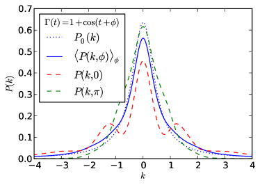
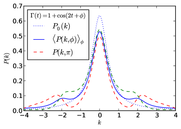
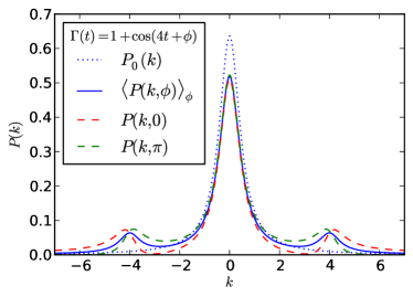
Figure 1: A two-level system decays into one photon. We plot the probability distribution function $P(k)$ of the photon’s momentum $k$, given by Eq. (40) with $j=1/2$, i.e. $P(k)=\mathcal{P}_{1}(k)$. The coupling strength $\Gamma$ is assumed to be time dependent, in particular oscillating, while the effective level-splitting $\Delta$ is set to zero. The probability distribution depends on the initial phase $\phi$ of $\Gamma(t)$. We plot $P(k)$ averaged over $\phi$, its value for $\phi=0,\pi$ and for comparison also the $\Gamma(t)=const.=1$ probability distribution $P_{0}(k)$. Note that the oscillation $\Gamma(t)=1+\cos(\Omega t+\phi)$ creates an additional peak at $k=\pm\Omega$.

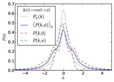
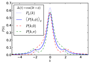
Figure 2: A two-level system decays into one photon. We plot the probability distribution function $P(k)$ of the photon’s momentum $k$, given by Eq. (40) with $j=1/2$, i.e. $P(k)=\mathcal{P}_{1}(k)$. The level-splitting $\Delta$ is assumed to be time dependent, in particular oscillating, while the coupling constant $g$ is assumed to be constant. The probability distribution depends on the initial phase $\phi$ of $\Delta(t)$. We plot $P(k)$ averaged over $\phi$, its value for $\phi=0,\pi$ and for comparison also the $\Delta(t)=const.=1$ probability distribution $P_{0}(k)$.

V Discussion and Conclusion

In this paper we discussed a path integral formulation for the lattice spin systems using the disentanglement procedure of the time-ordered exponential. This approach avoids using coherent states and is therefore free of their drawbacks. We invoked the stochastic formulation of the disentanglement procedure which effectively keeps all the non-differentiable paths, and thus is in principle exact. This allowed us to reproduce known results for a Bethe ansatz solvable model. Moreover we used the method to describe time-dependent parameters where the Bethe ansatz fails to provide a solution. From the fundamental point of view, the stochastic approach to the disentanglement equations reveals a hidden super-symmetric structure of the interacting spin system, and as a consequence leads to the effective action formulation in terms of the topological field theory. We believe that these new formulations could shed light on hidden topological and dynamical aspects of interacting lattice spin systems.

We comment here on possible further developments of our representation. The Riccati equation which plays a central role in the procedure has dynamical $sl(2)$ symmetry which could possibly help to select certain orbits in the path integral. For systems defined on higher rank algebras, such as $su(n)$, this equation becomes a matrix Riccati equation. The effective action in the stochastic formulation can be studied using both non-perturbative and perturbative techniques. Many of these approaches have been developed in the context of Onsager-Machlup theory for non-equilibrium stochastic processes, see e.g. work-relation ,ZJ . On the other hand, our very preliminary experience on numerical implementation of the method for generic spin system shows that large deviations ref:LargeDeviations1 will be an important obstacle to the numerical sampling of stochastic paths.

One more interesting question is how the integrability of certain lattice spin model (like e.g. XYZ spin chains) can be uncovered via our path-integral formulation. We envision interesting developments on this route.

VI Acknowledgement

We would like to thank Eugene Demler, Victor Galitski, Mikhail Kiselev, Mikhail Pletyukhov for many useful discussions and suggestions. The work was supported by the Swiss NSF.

VII Appendix

In this appendix we collect some relevant information about several parametrizations of the $SU(2)$ group and related Riemann and differential geometry notions mentioned in the main text.

VII.1 Different parametrizations of $SU(2)$

Here we overview various parametrizations of the group $SU(2)$ and present an explicit form of differential-geometric structures used in the main body of the paper.

The Caley-Klein parametrization

$$U(\alpha,\beta)=\left(\begin{array}[]{cc}\alpha&\beta\\ -\bar{\beta}&\bar{\alpha}\\ \end{array}\right),$$ (44)

where $|\alpha|^{2}+|\beta|^{2}=1$. This allows one to introduce new parameters $x_{1,\dots,4}$, $\alpha=x_{1}+ix_{2}$ and $\beta=x_{3}+ix_{4}$, which define an embedding of $S^{3}\simeq SU(2)$ to $R^{4}$. The underlying equations read

$$\phi_{3} = i(\dot{\alpha}\alpha+\dot{\beta}\beta)$$ (45)

$$\phi_{+} = i(-\dot{\alpha}\beta+\dot{\beta}\alpha),$$ (46)

and the complex conjugates of these two equations. Inverting them (when the determinant of the transformation is nonzero) yields

$$i\dot{\alpha} = \alpha\phi_{3}-\phi_{+}\bar{\beta}$$ (47)

$$i\dot{\beta} = \phi_{3}\beta+\phi_{+}\bar{\alpha}$$ (48)

The Euler parametrization is defined as

$$U(\alpha,\beta,\gamma)=e^{i\alpha(t)S^{3}}e^{i\beta(t)S^{2}}e^{i\gamma(t)S^{3}}.$$ (49)

Here $0\leq\alpha<2\pi$, $0\leq\beta\leq\pi$, and $0\leq\gamma\leq 4\pi$. The stochastic equations take the following form Chalker

$$\dot{\alpha} = -\phi_{1}(t)\cos\alpha\cot\beta-\phi_{2}(t)\sin\alpha\cot\beta+\phi_{3}(t)$$

$$\dot{\beta} = -\phi_{1}(t)\sin\alpha+\phi_{2}(t)\cos\alpha$$ (50)

$$\dot{\gamma} = \phi_{1}(t)\frac{\cos\alpha}{\sin\beta}+\phi_{2}(t)\frac{\sin\alpha}{\sin\beta}.$$

A rotationally invariant (covariant) parametrization is given by

$$U(t)=\exp(-i\psi{\bf n}\cdot{\bf S}),$$ (51)

where ${\bf n}(\theta,\phi)$ denotes a unit vector spanning a sphere. Its connection to the Euler parametrization is obtained easily by employing the lowest nontrivial representation — the Pauli matrix parametrization. It may be written as

$$\phi = \frac{1}{2}(\pi+\alpha-\gamma),$$

$$\tan\theta = \frac{\tan(\beta/2)}{\sin[\frac{1}{2}(\alpha+\gamma)]},$$ (52)

$$\cos\psi = 2\cos^{2}(\frac{\beta}{2})\cos^{2}(\frac{1}{2}(\alpha+\gamma))-1.$$ (53)

In this representation we define a vector ${\bf A}$ with three components $(A^{1},A^{2},A^{3})$ (don’t mix them up with parameters $A,B,C$ in the text for the other representation), by requiring that

$$U(t)=\exp(i\bm{\sigma}{\bf A}(t))$$ (54)

is the disentangled version of the $T$-ordered exponential. Using the standard formulas for the Pauli matrices we obtain

$$U(t)=\cos|A|+i\frac{\sin|A|}{|A|}(\bm{\sigma}{\bf A})$$ (55)

where $|A|$ is the length of the vector ${\bf A}$. Considering the time derivative $\partial_{t}U(t)$ and multiplying it by $U^{-1}(t)$ we get

$$-iU^{-1}\partial_{t}U(t) = \frac{|A|-\cos|A|\sin|A|}{|A|^{2}}\partial_{t}|A|(\bm{\sigma}\cdot{\bf A})$$

$$+ \frac{\cos|A|\sin|A|}{|A|}(\bm{\sigma}\cdot\partial_{t}{\bf A})$$

$$+ \frac{\sin^{2}|A|}{|A|^{2}}(\bm{\sigma}\cdot({\bf A}\times\partial_{t}{\bf A})),$$

which is to be then identified with the effective Hamiltonian $\bm{\phi}(t)\cdot\bm{\sigma}$. We therefore get a vector Langevin equation

$$\bm{\phi} = \frac{|A|-\cos|A|\sin|A|}{|A|^{2}}\partial_{t}|A|{\bf A}$$

$$+ \frac{\cos|A|\sin|A|}{|A|}\partial_{t}{\bf A}+\frac{\sin^{2}|A|}{|A|^{2}}({\bf A}\times\partial_{t}{\bf A}).$$

Note also that $(\bm{\phi}\cdot{\bf A})=\frac{1}{2}\partial_{t}|A|^{2}$. From this form it follows that the leading terms of a power expansion in terms of $|A|$ read $\bm{\phi}=\partial_{t}{\bf A}+{\bf A}\times\partial_{t}{\bf A}+\ldots$

The connection between different representations can be obtained by comparing their matrix forms with the one of the Caley-Klein:

$$\alpha = \cos\frac{|{\bf A}|}{2}+i\frac{A^{z}}{|{\bf A}|}\sin|{\bf A}|$$ (58)

$$\beta = i\frac{A_{x}-iA_{y}}{|{\bf A}}\sin|{\bf A}|,$$ (59)

while for the Gauss parametrization, $\exp(-B/2)=\bar{\alpha}$.

VII.1.1 Various disentangling formulas

Let $S_{\pm,0}$ be the generators of $su(2)$ or $su(1,1)$, so that $[S_{-},S_{+}]=2\sigma S_{0}$ and $[S_{0},S_{\pm}]=\pm S_{\pm}$, where $\sigma=1$ for the $su(1,1)$ and $\sigma=-1$ for the $su(2)$. The Casimir invariant is therefore $C_{2}=S_{0}^{2}-\frac{\sigma}{2}(S_{+}S_{-}+S_{-}S_{+})$. The evolution operator can be written in a variety of forms distinguished by a different ordering of terms containing $S_{\pm,0}$. These include the symmetric form,

$$U_{S}=\exp(a_{+}S_{+}+a_{0}S_{0}+a_{-}S_{-})$$ (60)

the normal-ordered Cartan form

$$U_{N}=\exp(A_{+}S_{+})\exp(\log[A_{0}]S_{0})\exp(A_{-}S_{-})$$ (61)

or the anti-normal-ordered Cartan form

$$U_{A}=\exp(B_{-}S_{-})\exp(\log[B_{0}]S_{0})\exp(B_{+}S_{+}).$$ (62)

They are related as follows ban :

$$A_{\pm} = \frac{\frac{a_{\pm}}{D}\sinh D}{\cosh D-\frac{a_{0}}{2D}\sinh D},$$

$$A_{0} = \left(\cosh D-\frac{a_{0}}{2D}\sinh D\right)^{2}$$

$$B_{\pm} = \frac{\frac{a_{\pm}}{D}\sinh D}{\cosh D+\frac{a_{0}}{2D}\sinh D},$$

$$B_{0} = \left(\cosh D+\frac{a_{0}}{2D}\sinh D\right)^{2}$$ (63)

and

$$A_{0}=\frac{B_{0}}{(1-\sigma B_{+}B_{-}B_{0})^{2}},\quad A_{\pm}=\frac{B_{\pm}B_{0}}{1-\sigma B_{+}B_{-}B_{0}}$$

$$B_{0}=\frac{(A_{0}-\sigma A_{+}A_{-})^{2}}{A_{0}},\quad B_{\pm}=\frac{A_{\pm}}{A_{0}-\sigma A_{+}A_{-}}$$ (64)

where $D=\frac{1}{2}(a_{0}^{2}-4\sigma a_{+}a_{-})^{1/2}$.

The ordered product of arbitrary number of symmetric operators, $U_{S}(n)=\exp(a_{+}(n)J_{+}+a_{0}(n)J_{0}+a_{-}(n)J_{-})$ labeled by some discrete index $n=1,\ldots N$,

$$U_{S}(N)=\prod_{n=1}^{N}U_{S}(n)=U_{S}(N)U_{S}(N-1)\ldots U_{S}(1)$$ (65)

can be represented in any of the forms above. In particular, for any $n$ the normal ordered form

$$U_{S}(n)=\exp(A_{+}(n)S_{+})\exp(A_{0}(n)S_{0})\exp(A_{-}(n)S_{-}),$$

can be obtained recursively using the quantities $A_{\pm,0}(n-1)$ defined at the previous discretization step $n-1$ and the quantities $a_{\pm,0}(N)$ defined at the step $n$. The explicit formulas are stated in ban .

VII.2 Connection between group-theoretic and geometric approaches: example of $SU(2)$

For the group $SU(2)$ we define $[t^{a},t^{b}]=i\epsilon^{abc}t^{c}$. A basis for the algebra can be taken to be a set of Pauli matrices. We have for the arbitrary element of $g\in G$, $g^{-1}dg=\sum_{a}\omega_{a}t_{a}$, where $\omega_{a}$ is the Maurer-Cartan form. These 1-forms satisfy $d\omega_{a}+\frac{1}{2}f_{abc}\omega_{b}\wedge\omega_{c}=0$, because of the identity $d(g^{-1}dg+g^{-1}dg\wedge g^{-1}dg=0$. Parametrizing $SU(2)$ as $\alpha=\cos(u_{1}/2)\exp(i(u_{2}+u_{3})/2)$, $\beta=i\sin(u_{1}/2)\exp(i(u_{2}-u_{3})/2)$, the 1-form becomes

$$\frac{i}{2}\left(\begin{array}[]{cc}du_{3}+\cos u_{1}du_{1}&e^{-iu_{3}}(du_{1}+idu_{2}\sin u_{1}\\ e^{iu_{3}}(du_{1}-idu_{2}\sin u_{1}&-du_{3}-\cos u_{1}du_{1}\\ \end{array}\right).$$ (68)

This means that

$$\omega_{1} = \cos u_{3}du_{1}+\sin u_{3}\sin u_{1}du_{2}$$

$$\omega_{2} = \sin u_{3}du_{1}-\cos u_{3}\sin u_{1}du_{2}$$

$$\omega_{3} = \cos u_{1}du_{2}+du_{3}.$$ (69)

Using these equations, one can readily check the Maurer-Cartan equation, $d\omega_{a}+\frac{1}{2}\epsilon_{abc}\omega_{b}\wedge\omega_{c}$.

Geometrically speaking, $SU(2)$ is equivalent to $S^{3}$. The metric induced on it by the embedding into $R^{4}=C^{2}$ can be found easily,

$$ds^{2}=du_{1}^{2}+du_{2}^{2}+du_{3}^{2}+2\cos u_{1}du_{2}du_{3}.$$ (70)

The determinant of the metric $\det(g_{\mu\nu})=sin^{2}u_{1}$ and therefore the volume of the $S^{3}$ is normalized as $\int_{SU(2)}\det^{1/2}(g_{\mu\nu})du_{1}du_{2}du_{3}=16\pi^{2}$, the inverse of the metric yields

$$g^{\mu\nu}=\left(\begin{array}[]{ccc}1&0&0\\ 0&\csc^{2}u_{1}&-\cot u_{1}\csc u_{1}\\ 0&-\cot u_{1}\csc u_{1}&\csc^{2}u_{1}\\ \end{array}\right),$$ (74)

and nonzero Christoffel symbols read

$$\Gamma^{1}_{23} = \frac{1}{2}\sin u_{1},\qquad\Gamma^{2}_{13}=\Gamma^{3}{12}=\frac{-1}{2\sin u_{1}},$$

$$\Gamma^{3}_{13} = \Gamma^{2}{12}=\frac{1}{2}\cot u_{1}.$$ (75)

The dreibein on $S^{3}$ is equal to $\omega$ within our normalization (otherwise there may arise a proportionality factor),

$$e^{a}_{\mu}=(\omega_{a})_{\mu},\qquad e^{a}=e^{a}_{\mu}dx^{\mu}=\omega_{a}.$$ (76)

One can check that

$$e^{a}_{\mu}e^{b}_{\nu}\eta_{ab}=g_{\mu\nu}.$$ (77)

The inverse dreibein is

$$E^{\mu}_{a}=\eta_{ab}g^{\mu\nu}e^{b}_{\mu}$$ (78)

and is used to define left-invariant vector fields

$$l_{a}=E^{\mu}_{a}\frac{\partial}{\partial x^{\mu}},$$ (79)

which in this case are

$$l_{1} = \cos u_{3}\frac{\partial}{\partial u_{1}}+\frac{\sin u_{3}}{\sin u_{1}}\frac{\partial}{\partial u_{2}}-\sin u_{3}\cot u_{1}\frac{\partial}{\partial u_{3}}$$

$$l_{2} = \sin u_{3}\frac{\partial}{\partial u_{1}}-\frac{\cos u_{3}}{\sin u_{1}}\frac{\partial}{\partial u_{2}}+\cos u_{3}\cot u_{1}\frac{\partial}{\partial u_{3}}$$

$$l^{3} = \frac{\partial}{\partial u_{3}}.$$ (80)

One can see that $e^{a}(l_{b})=\delta^{a}_{b}$ and that these vector fields form the $su(2)$ algebra themselves. The spin connection satisfies $de^{a}+\omega^{a}_{b}\wedge e^{b}=0$ and is given explicitly by equations

$$\omega^{a}_{b\mu} = -E^{\nu}_{b}(\partial_{\mu}e^{a}_{\nu}-\Gamma^{\lambda}_{\mu\nu}e^{a}_{\lambda}),$$

$$\partial_{\mu}e^{a}_{\nu} = \Gamma^{\lambda}_{\mu\nu}e^{a}_{\lambda}-e^{b}_{\nu}\omega^{a}_{b\mu}$$ (81)

$$\omega^{a}_{b} = \epsilon^{a}_{bc}e^{c}.$$

The Laplace-Beltrami operator yields $\Delta_{LB}=l_{a}^{2}$.

All the expressions above are representation-dependent. In particular, in the representation defined by the Cartan decomposition we have

$$g_{G} = e^{\psi S_{-}}e^{\phi S_{z}}e^{\chi S_{+}}$$ (82)

$$= \left(\begin{array}[]{cc}1&0\\ \psi&1\\ \end{array}\right)\left(\begin{array}[]{cc}e^{\phi}&0\\ 0&e^{-\phi}\\ \end{array}\right)\left(\begin{array}[]{cc}1&\chi\\ 0&1\\ \end{array}\right),$$ (89)

and the Maurer-Cartan currents are given by

$$g^{-1}dg = \left(\begin{array}[]{cc}-e^{2\phi}\chi d\psi+d\phi&-e^{2\phi}\chi^{2}d\psi+2\chi d\phi+d\chi\\ e^{2\phi}d\psi&e^{2\phi}\chi d\psi-d\phi\\ \end{array}\right),$$ (92)

$$dgg^{-1} = \left(\begin{array}[]{cc}-e^{2\phi}\psi d\chi+d\phi&e^{2\phi}d\chi\\ -e^{2\phi}\psi^{2}d\chi+2\psi d\phi+d\psi&e^{2\phi}\psi d\chi-d\phi\\ \end{array}\right),$$ (95)

while the left-invariant vector fields read

$$l_{+} = \frac{\partial}{\partial\chi},\quad l_{3}=-2\chi\frac{\partial}{\partial\chi}+\frac{\partial}{\partial\phi},,$$

$$l_{-} = e^{-2\phi}\frac{\partial}{\partial\psi}+\chi\frac{\partial}{\partial\phi}-\chi^{2}\frac{\partial}{\partial\chi}$$ (96)

and the right-invariant fields yield

$$r_{+} = \frac{\partial}{\partial\psi},\quad r_{3}=-2\psi\frac{\partial}{\partial\psi}+\frac{\partial}{\partial\phi},,$$

$$r_{-} = e^{-2\phi}\frac{\partial}{\partial\chi}+\psi\frac{\partial}{\partial\phi}-\psi^{2}\frac{\partial}{\partial\psi}.$$ (97)

The components of the vielbein can be read off these results straightforwardly. Validity of the Maurer-Cartan equation can also be checked. Also note that $(g^{-1}dg)^{a}r_{b}=\delta^{a}_{b}$, and $(dgg^{-1})^{a}l_{b}=\delta^{a}_{b}$.

VII.3 Discretized version of the disentangling equations in the stochastic formulation

If one wants to interpret the equations as stochastic differential equations with respect to the Wiener process, one should look into the exact discretization outlined in Eqs. (65), and explicitly in Ref. ban . Let us split $\phi_{\pm,3}$ into a white-noise and deterministic part, i.e. define $\phi_{\pm,3}=\sqrt{\varepsilon}\varphi_{\pm,3}+\varepsilon h_{\pm,3}=dR_{\pm,3}+h_{\pm,3}dt$. For convenience we denote the discretized versions of $\xi_{+}(t),\xi_{-}(t),\xi_{z}(t)$ as $A_{n},C_{n},B_{n}$, respectively. The discretized equations then take the following form:

$$A_{n+1} = A_{n}+\sqrt{\varepsilon}\left(\varphi_{+,n}+A_{n}\varphi_{3,n}-A_{n}^{2}\varphi_{-,n}\right)$$

$$+ \varepsilon\left(h_{+,n}+A_{n}h_{3,n}-A_{n}^{2}h_{-,n}\right)+$$

$$+ \frac{\varepsilon}{2}(\varphi_{+,n}\varphi_{3,n}+A_{n}\varphi_{3,n}^{2}-2A_{n}\varphi_{+,n}\varphi_{-,n}$$

$$- 3A_{n}^{2}\varphi_{3,n}\varphi_{-,n}+2A_{n}^{3}\varphi_{-,n}^{2})+o(\varepsilon)$$

$$C_{n+1} = C_{n}+\sqrt{\varepsilon}e^{B_{n}}\varphi_{-,n}$$

$$+ \varepsilon e^{B_{n}}\left(h_{-,n}+\frac{1}{2}\varphi_{3,n}\varphi_{-,n}-A_{n}\varphi_{-,n}^{2}\right)+o(\varepsilon)$$

$$e^{B_{n+1}} = e^{B_{n}}+\sqrt{\varepsilon}e^{B_{n}}(\varphi_{3,n}-2A_{n}\varphi_{-,n})$$

$$+ \varepsilon e^{B_{n}}(h_{3,n}-2A_{n}h_{-,n}+\frac{1}{2}\varphi_{3,n}^{2}-\varphi_{+,n}\varphi_{-,n}$$

$$- 3A_{n}\varphi_{3,n}\varphi_{-,n}+3A_{n}^{2}\varphi_{-,n}^{2})+o(\varepsilon).$$

These equations form the basis for the construction of the corresponding SDEs. The particular form of the equations clearly depends on the particular properties of the noises. For a general model with the quadratic coupling $\frac{1}{2}\Omega_{ij}\left(\gamma_{x}S^{x}_{i}S^{x}_{j}+\gamma_{y}S^{y}_{i}S^{y}_{j}+\gamma_{z}S^{z}_{i}S^{z}_{j}\right)$ the noise action is $\frac{1}{2}\Omega^{-1}_{ij}(\gamma^{-1}_{x}\varphi^{x}_{i}\varphi^{x}_{j}+\gamma^{-1}_{y}\varphi^{y}_{i}\varphi^{y}_{j}+\gamma^{-1}_{z}\varphi^{z}_{i}\varphi^{z}_{j})$. The noises are thus $\varphi_{\pm}=\frac{1}{2}(\varphi_{x}\mp i\varphi_{y})$, $\varphi_{3}=\varphi_{z}$. If the noises $dR_{\pm,3}$ are independent, we can rewrite the relations in the form of Ito SDE,

$$dA = (h_{+}+Ah_{3}-h_{-}A^{2}$$

$$- \frac{K}{4}A(\gamma_{x}(1-A^{2})+\gamma_{y}(1+A^{2})-2\gamma_{z}))dt$$

$$+ \frac{1}{2}(1-A^{2})dR_{x}-\frac{i}{2}(1+A^{2})dR_{y}+AdR_{3}$$

$$dC = e^{B}(h_{-}-\frac{K}{4}A(\gamma_{x}-\gamma_{y}))dt$$

$$+ \frac{1}{2}e^{B}(dR_{x}+idR_{y})$$

$$de^{B} = e^{B}(h_{3}-2Ah_{-}$$

$$+ \frac{K}{4}(2\gamma_{z}+\gamma_{x}(3A^{2}-1)-\gamma_{y}(3A^{2}+1)))dt$$

$$+ e^{B}(dR_{3}-A(dR_{x}+idR_{y})),$$

Here we assume that the noises $dR$ can be written in terms of unit Wiener processes $dW$ via $dR_{x,y,z}=\sqrt{\gamma_{x,y,z}}\sum_{i}T_{il}dW_{l;x,y,z}$. The constant $K$ in Eqs. (VII.3) is expressed via $T_{ij}$ as $K:=\sum_{l}T_{il}^{2}$. The matrix $T_{ij}$ can be straightforwardly related to the inverse of the matrix $O_{ij}$ defined above Eq. (15). These equations can be casted into a much simpler form by utilizing the Stratonovich interpretation:

$$dA=\left(h_{+}+Ah_{3}-h_{-}A^{2}\right)dt$$

$$+\frac{1}{2}(1-A^{2})dR_{x}-\frac{i}{2}(1+A^{2})dR_{y}+AdR_{3}$$

$$dC=e^{B}\left(h_{-}\right)dt+\frac{1}{2}e^{B}\left(dR_{x}+idR_{y}\right)$$ (100)

$$de^{B}=e^{B}\left(h_{3}-2Ah_{-}\right)dt+e^{B}\left(dR_{3}-A(dR_{x}+idR_{y}\right)).$$

Further insight may into the SDE interpretation of the equations may be obtained from Figs. 3 and 4, where we present numerical results for a 1D Ising chain of $N=16$ spins in the transversal magnetic field $h$, simulated in the imaginary time $\tau$. These figures display typical trajectories of the local function $A_{1}$ (thanks to the translational invariance, we may choose any site), as well as its probability distribution. Let us note that the stochastic process $A$ becomes stationary at large imaginary times, obeying the log-normal distribution.

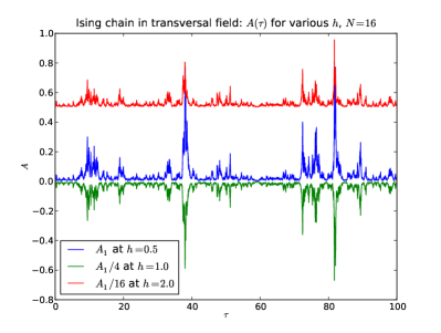
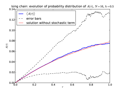
Figure 3: Upper panel: Typical realizations of the stochastic process $A_{1}(\tau)$, in imaginary time $\tau$ for various magnetic fields $h$. Values of $A_{1}$ for different $h$s are rescaled, mirrored and shifted to improve their visibility. The magnitude of $A$ scales approximately as $h^{2}$. Trajectories are all taken for the same noise realization, so that one can compare the influence of a fluctuation in noise on the solution $A$ at different $h$. Lower panel: Initial part of the evolution of $A_{1}(\tau)$. The red line is a solution of the underlying SDEs neglecting the contributions of the noise term. The blue line is an average of solutions, averaged over 1000 realizations of the noise. Dashed lines represent error bounds given by $\sqrt{\mathrm{var}A(\tau)}$. We can clearly see the crossover from the “deterministic” region at small $\tau$ into a purely stochastic stationary regime at larger $\tau$.

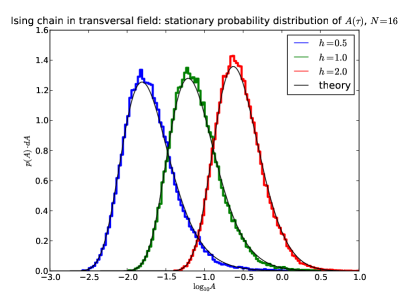
Figure 4: Upper panel: The time evolution of the probability distribution of $A_{1}(\tau)$. The histograms are plotted for 1000 realizations of the process with the magnetic field $h=0.5$. Lower panel: The empirical histograms of $A_{1}$ after the distribution becomes stationary (for large enough $\tau$, vs. the asymptotic log-normal probability distribution, plotted for several magnetic fields $h$. Note that the horizontal axis is plotted in the $\log$ scale. The histograms shown in the left panel converge for large times $\tau$ to the ones in the lower panel.

References

• (1) H. Kleinert, Path Integrals in Quantum Mechanics, Statistics, Polymer Physics, and Financial Markets, (World Scientific, Singapore, 2009)
• (2) J. Zinn-Justin, Quantum Field theory and Critical phenomena (Oxford UP 2002).
• (3) J. W. Negele, H. Orland, Quantum Many Particle Systems (Westview Press, 1998).
• (4) E. Fradkin, Field Theories of Condensed Matter Physics, (Cambridge UP 2013)
• (5) V. I. Yudson, and P. Reineker, Phys. Rev. A 78, 052713 (2008); V. I. Rupasov and V. I. Yudson, Zh. Eksp. Teor. Fiz. 87, 1617 (1984) [Sov. Phys. JETP 60, 927 (1984)]; V. I. Rupasov and V. I. Yudson, Zh. Eksp. Teor. Fiz. 86, 819 (1984) [Sov. Phys. JETP 59, 478 (1984)]; V. I. Yudson, Zh. Eksp. Teor. Fiz. 88, 1757 (1985) [Sov. Phys. JETP 61, 1043 (1985)].
• (6) E. Witten, Commun. Math. Phys. 117, 353 (1988); 118, 411 (1988).
• (7) E. Frenkel, A. Losev, N. Nekrasov, arXiv:hep-th/0610149, arXiv:hep-th/0702137, arXiv:0803.3302; A. Losev, S. Slizovskiy, J.Geom.Phys. 61, 1868 (2011).
• (8) J. Hubbard, Phys. Lett. 3, 77 (1959).
• (9) A. Perelomov, Generalized coherent states and their applications, (Springer, 1986).
• (10) I. S. Burmistrov, Y. Gefen, and M. N. Kiselev, Pis’ma v ZhETF 92, 202 (2010).
• (11) I. S. Burmistrov, Y. Gefen, and M. N. Kiselev, Phys. Rev. B 85, 155311 (2012).
• (12) I. V. Kolokolov, Phys. Lett. A 114, 99 (1986).
• (13) I. V. Kolokolov, Ann. Phys. 202, 165 (1990).
• (14) M. Chertkov, and I.V. Kolokolov, Phys. Rev. B 51, 3974 (1995).
• (15) M. Chertkov, and I.V. Kolokolov, Sov. Phys. JETP 79, 824 (1994).
• (16) I. V. Kolokolov, JETP 76, 1099 (1993).
• (17) I. V. Kolokolov, Int. J. Mod. Phys. B 10, 2189 (1996).
• (18) P. M. Hogan and J. T. Chalker, J. Phys. A: Math. Gen. 37, 11751 (2004).
• (19) V. Galitski, Phys. Rev. A 84, 012118 (2011).
• (20) M. Ringel, V. Gritsev, EPL 99, 20012 (2012).
• (21) J. Wei, E. Norman, J. Math. Phys. 4, 575 (1963).
• (22) V. G. Kac, Infinite-dimensional Lie algebras, (Birkhäuser, 1983).
• (23) A. A. Kirillov, Elements of the Theory of Representations, (Springer, 1976).
• (24) C. S. Gardner, J. M. Greene, M. D. Kruskal, R. M. Miura, Phys. Rev. Lett. 19, 1095 (1967)
• (25) F. Langouche, D. Roekaerts, and E. Tirapegui, Functional Integration and Semiclassical Expansions (Reidel, Dordrecht, 1982); H. Calisto, and E. Tirapegui, Phys. Rev. E 65, 038101 (2002).
• (26) P. Arnold, Phys. Rev. E 61, 6091 (2000); 61, 6099 (2000).
• (27) C. Becchi, A. Rouet, R. Stora, Ann. Phys. 98, 287 (1976); I.V. Tyutin, Lebedev Physics Institute preprint 39 (1975), arXiv:0812.0580.
• (28) G. Parisi, N. Sourlas, Nucl. Phys. B 206, 321 (1982).
• (29) M. V. Feigelman, A. M. Tsvelik, JETP 83, 1430 (1982).
• (30) D. Hochberg, C. Molina-Paris, J. Perez-Mercader, M. Visser, Phys. Rev. E 60, 6343 (1999); K. Mallick, M. Moshe, H. Orland, J. Phys. A 44, 095002 (2011).
• (31) D. Friedan, A. Konechny, Adv. Theor. Math. Phys. 13 (2009)
• (32) G. Parisi, N. Sourlas, Phys. Rev. Lett. 43, 744 (1979).
• (33) I. V. Ovchinnikov, Chaos 22, 033134 (2012); arXiv:1212.1989.
• (34) T. Shi, and C. P. Sun, Phys. Rev. A 76, 062709 (2007).
• (35) T. Shi, and C. P. Sun, Phys. Rev. B 79, 205111 (2009).
• (36) T. Shi, S. Fan, and C. P. Sun, Phys. Rev. A 84, 063803 (2011).
• (37) H. Lehmann, K. Symanzik, and W. Zimmermann, Nuovo Cimento 1, 205 (1955).
• (38) C. W. Gardiner, Handbook of Stochastic Methods (Springer-Verlag, 2004).
• (39) S. De Liberato, D. Gerace, I. Carusotto, and C. Ciuti, Phys. Rev. A 80, 053810 (2009).
• (40) D. A. Fuhrmann, et al., Nature Photonics 5, 605 (2011).
• (41) H. Touchette, Physics Reports 478, 1 (2009)
• (42) M. Ban, J. Opt. Soc. Am. B 10, 1347 (1993).