Classification and environmental properties of X-ray selected point-like sources in the XMM-LSS field

Abstract

Context. The XMM-Large Scale Structure survey, covering an area of 11.1 sq. deg., contains more than 6000 X-ray point-like sources detected with XMM-Newton down to a flux of $3\times 10^{-15}$ erg s^-1 cm^-2 in the [0.5-2] keV band, the vast majority of which have optical (CFHTLS), infrared (SWIRE IRAC and MIPS), near-infrared (UKIDSS) and/or ultraviolet (GALEX) counterparts.

Aims. We wish to investigate the environmental properties of the different types of the XMM-LSS X-ray sources, defining their environment using the $i^{\prime}$-band CFHTLS W1 catalog of optical galaxies down to a magnitude limit of 23.5 mag.

Methods. We have classified 4435 X-ray selected sources on the basis of their spectra, SEDs and X-ray luminosity and estimated their photometric redshifts, having 4-11 band photometry, with an accuracy $\sigma_{\triangle z/(1+z_{sp})}$=0.076 and 22.6% outliers for $i^{\prime}<$26 mag. We estimated the local overdensities of 777 X-ray sources which have spectro-z or photo-z calculated using more than 7 bands (accuracy $\sigma_{\triangle z/(1+z_{sp})}$=0.061 with 13.8% outliers) within the volume-limited region defined by $0.1\leq z\leq 0.85$ and -23.5$<M_{i^{\prime}}<$-20.

Results. Although X-ray sources may be found in variety of environments, a large fraction ($\sim$$>$ 55-60%), as verified by comparing with the random expectations, reside in overdense regions. The galaxy overdensities within which X-ray sources reside show a positive recent redshift evolution (at least for the range studied; $z\raise-3.0pt\hbox{\hbox to0.0pt{\hbox{$\sim$}\hss}\raise 4.0pt\hbox{$<$}\ }0.85$). We also find that X-ray selected galaxies, with respect to AGN, inhabit significantly higher galaxy overdensities, although their spatial extent appear to be smaller than that of AGN. Hard AGN ($HR\geq-0.2$) are located in more overdense regions with respect to the Soft AGN ($HR<-0.2$), a fact clearly seen in both redshift ranges, although it appears to be stronger in the higher redshift range ($0.55<z<0.85$). Furthermore, the galaxy overdensities (with $\delta\raise-3.0pt\hbox{\hbox to0.0pt{\hbox{$\sim$}\hss}\raise 4.0pt\hbox{$>$}\ }1.5$) within which Soft AGN are embedded appear to evolve more rapidly with respect to the corresponding overdensities around Hard AGN.

1 Introduction

Active galactic nuclei (AGN) are among the most powerful energy emitters in the Universe and trace the locations of active supermassive black holes (SMBHs) on the cosmic web. Understanding the nature and evolution of SMBHs as a function of cosmic time and environment constitutes an important goal of modern high-energy astrophysics. In particular the coincidence between the star-formation peak of galaxies at redshifts $z\sim$2-3 and the corresponding formation peak of high-luminosity AGN/QSOs, appears to link in an intricate way the cosmic histories of galaxies and black holes, providing an important input in understanding the formation and evolution of cosmic structures in the Universe (Warren et al. 1994; Schawinski et al. 2009; Fanidakis et al. 2012).

It is known that environmental effects (cf. interactions, minor or major galaxy merging) may affect the physical properties of galaxies such as their morphological type, color, star-formation rate, nuclear activity, etc. (Dressler 1980, Blanton et al. 2003a, Kauffmann et al. 2004, van der Wel 2008, etc.). The connection between galaxy and black hole formation and evolution indicates that there must be a dependence of the physical properties of AGN and of their triggering mechanism on environment, which has to be clearly established. Important questions are: (a) what is the main determining factor of the galaxy/AGN properties: intrinsic evolution or environmental influence? and (b) how do the host galaxy physical properties and the local environment affect the black hole fuelling mechanisms? To answer these questions, many authors have been studying the properties of AGN environment (density, colors, morphology, etc. of the nearest neighbours) and compared these properties with those of normal galaxies.

For example, Kauffmann et al. (2004) conclude that for a fixed stellar mass of galaxies, both star formation and nuclear activity strongly depend on the environment up to $\sim$1 Mpc. Waskett et al. (2005) did not find any differences between the environmental properties of AGN and of a control sample of galaxies in the 0.4$<z<$0.6 redshift range. A qualitatively similar result was obtained by Li et al. (2006) analyzing the clustering properties of narrow-line AGN. Gilmour et al. (2007) considered the environment of X-ray selected AGN in the supercluster A901/2 (at z=0.17) and found that they prefer dense environments, avoiding however the most overdense and underdense regions. Similarly, Lietzen et al. (2009) using SDSS data found that QSOs avoid the densest regions and prefer to reside in the outskirts of superclusters. Constantin et al. (2008) find that local ($z\raise-3.0pt\hbox{\hbox to0.0pt{\hbox{$\sim$}\hss}\raise 4.0pt\hbox{$<$}\ }0.09$) AGN are more common in voids than in walls for a same range of masses and accretion rates. The recent analysis of Lietzen et al. (2011) shows that radio-quiet QSOs and Seyfert galaxies prefer low-density regions contrary to radio galaxies which prefer more dense environments.

Silverman et al. (2009), on the basis of X-ray selected AGN in the COSMOS field, reached the conclusion that AGN prefer to reside in environments which are similar to those of massive galaxies with substantial levels of star formation. The AGN with low stellar mass hosts are located over a wide range of environments but AGN with high stellar mass hosts prefer low density regions. These results are also in agreement with Montero-Dorta et al. (2009) who found that Seyferts and X-ray selected AGN at z$\sim$1 almost do not show environmental dependencies. Moreover low-redshift LINERs and Seyfert galaxies appear to inhabit low density environments contrary to high-redshift LINERs (z$\sim$1) which favour higher density environments. Contrary to this, Georgakakis et al. (2007; 2008) found that the X-ray population at $z\sim$1 avoids underdense regions and prefers to reside in groups. Falder et al. (2010) showed that $z\sim 1$ AGN have an excess of galaxy density within a radius of 200-300 kpc and that the local galaxy density increases with the radio AGN luminosity, but not with the black hole mass. Bradshaw et al. (2011) showed that X-ray and radio-loud AGN, with 1.0$<z<$1.5, are located in significantly overdense regions, with the former being found in the cluster outskirts. Furthermore, recent clustering studies of X-ray selected AGN have shown that they reside in group-size dark matter halos with masses $M_{h}\sim 10^{13}h^{-1}M_{\odot}$, significantly more massive than those inhabited by optical QSOs (see Miyaji et al. 2011; Allevato et al. 2011, Koutoulidis et al. 2012, and references therein).

According to the unified scheme of Antonucci (1993), AGN of different types, like Seyferts of type I and II as well as broad and narrow line QSOs (unobscured and obscured ones), should inhabit similar environments since these objects only differ due to differences in orientation of their torus with respect to the line-of-sight. However the standard orientation-based AGN unification scheme does not consider any evolution with redshift of the properties of obscured vs. unobscured AGN. Is there some observational evidence establishing a similar environment for the different types of AGN? Statistical studies lead to contradictory results.

Koulouridis et al. (2006) found in the very local Universe that the fraction of Seyfert 2 galaxies with close neighbours is significantly larger than that of their control sample and of Seyfert 1 galaxies, while their large scale environment does not show any difference with respect to their control samples (see also Sorrentino et al. 2006 for similar results). At the same time, Strand et al. (2008) have shown that higher luminosity AGN inhabit more overdense environments compared to lower luminosity AGN out to 2 Mpc. The authors also found that in the redshift range 0.3$<z<$0.6, type II and type I QSOs present similarly overdense environments, while the environment of dimmer type I quasars appears to be less overdense than that of type II quasars.

X-ray selected sources which mainly consist of AGN offer information about the nature and properties of super massive black holes over a wide redshift range up to z$\sim$4. Therefore X-ray surveys combined with a multiwavelength analysis of their host galaxies provide an effective tool for the environmental study of different types of AGN. In our work we consider the environmental vs. intrinsic properties of X-ray selected, but with optically detected counterparts, point-like sources from the 11.1 sq. deg XMM-Large Scale Structure (LSS) medium-deep extragalactic survey. Earlier versions of our survey, over a smaller solid angle, and a variety of analyses can be found in Chiappetti et al. (2005), Gandhi et al. (2006), Pierre et al. (2007), Tajer et al. (2007), Polletta et al. (2007), Garcet et al. (2007), Tasse et al. (2008a,b) and Nakos et al. (2009).

In particular, regarding previous environmental studies based on the original XMM-LSS field, Tasse et al. (2008b) considered the environment of 110 radio-loud AGN finding that high and low stellar mass systems are located in different environments. The authors concluded that the AGN triggering mechanism of high mass systems could be produced by cooling of the hot gas and for the low mass systems it can be explained by the cold gas accretion due to a merging. In addition, Tasse et al. (2011) found that X-ray selected type 2 AGN show very similar individual and environmental properties as low mass radio-loud AGN.

The main aim of our current work is to consider the environmental properties of different types of X-ray selected XMM-LSS sources using the local density of optical galaxies based on the CFHTLS. In our analysis we use the newest version of the XMM-LSS multiwavelength catalog (Chiappetti et al. 2012) which contains 6342 X-ray sources over 11.1 sq. deg. The clustering properties of the point-like sources of this catalog were analyzed by Elyiv et al. (2012).

In section 2 we present the XMM-LSS source sample. In Section 3, we discuss the classification of the optical counterparts, the photo-$z$ determination technique and the corresponding results. Section 4 presents the multiwavelength properties of the sources and the samples of the different types of X-ray sources. The results of the environmental analysis are given in Section 5. Discussion and general conclusions form Section 6. Throughout this work we use the standard cosmology: $\Omega_{0}$=0.3, $\Omega_{\Lambda}$=0.7 and $H_{0}$=72 km/s/Mpc.

2 The sample of X-ray sources and their counterparts

The XMM-LSS field occupies an area of 11.1 sq. deg. and is located at high galactic latitudes by [2${}^{h}14^{m}<R.A.<2^{h}30^{m}$; -6$\raisebox{4.30554pt}{\scriptsize o}25^{m}<Dec<-2\raisebox{4.30554pt}{\scriptsize o}35^{m}$, J2000.0], see Fig. 1. This field also contains the Subaru X-ray Deep Survey (SXDS) 1.14 sq. deg. deep field (Ueda et al. 2008). We will refer below to the XMM-LSS field as the “Full Exposure Field” which includes the SXDS field.

The XMM-LSS full exposure field contains 6342 sources² detected in the soft (0.5-2 keV) and/or hard (2-10 keV) bands down to a detection likelihood of 15. This corresponds to the following flux limits (50% detection probability): F${}_{(0.5-2keV)}=3\times 10^{-15}$ erg s^-1 cm^-2 and F${}_{(2-10keV)}=1\times 10^{-14}$ erg s^-1cm^-2, over nominal survey pointings.

See further details about the catalog sensitivity in Elyiv et al. (2012) and the catalog description paper by Chiappetti et al. (2012). In the latter paper the details of the soft and hard band ”merging” are also given. From the multiwavelength catalog of the X-ray point-like sources and their counterparts in optical/CFHTLS, infrared/SWIRE/IRAC and MIPS, near-infrared UKIDSS and ultraviolet GALEX, we only selected those sources which have a counterpart at optical wavelength or more wavelengths. The detailed description of the matching of X-ray sources with their multiwavelength counterparts is given in Chiappetti et al. (2012).

We only took one counterpart for each X-ray source; that which had the best $probXO$ probability (see definition below) and rank 0 (single counterpart) or 1 (preferred counterpart but there are more than one), see Chiappetti et al. (2012) for details. The total number of X-ray selected sources with corresponding counterparts is 5142.

Each counterpart was visually inspected using CFHTLS $g^{\prime}$, $i^{\prime}$, $r^{\prime}$ images from the 6^th release by two independent inspectors. The majority of the counterparts have $g^{\prime}$ and $r^{\prime}$-band observations: 5078 sources are visible in $g^{\prime}$ and 5047 in the $r^{\prime}$-band, respectively. According to our rough visual classification the sources were split into extended sources ($ext$), point-like sources ($ptl$), the latter consisting mostly of QSOs, stars. We reserved one more category for very faint/invisible objects, photo-defects, etc. These objects are referred as misclassified objects $mcl$. The top and middle panels of Fig. 2 show the distribution of sources as a function of their apparent $r^{\prime}$ magnitude according to the two independent inspectors. The second inspector tends to classify faint objects and objects with bright nuclei as $ptl$, while the first inspector classifies most of these objects as extended ones ($ext$). Similar types were assigned for about 90% of objects up to $\sim$22 mag by both inspectors (see the bottom panel of Fig. 2).

Therefore we preliminary considered 2441optical counterparts as $ext$ (if at least one inspector marks the object as $ext$), 2280 as $ptl$ (if both inspectors classify the object as $ptl$) and rejected from any further consideration 238 $mcl$ and 183 stars (83 of them are spectroscopically confirmed and the rest confirmed from their SEDs, see section 3). From both visual classifications it is clearly seen that stars typically have magnitudes less than $\sim$16 mag and $mcl$ counterparts are dominating the sources with magnitudes above $\sim$25 mag. Such a kind of visual inspection was necessary to reject ”bad” counterparts and to have an idea on how to choose the photometric templates. The final classification of the sources was made on the basis of spectroscopic information, SEDs and/or X-ray luminosities (see section 3 and subsection 4.1 for the details).

In the XMM-LSS catalogs (Chiappetti et al. 2005, 2012, Pierre et al. 2007), each selected multiwavelength counterpart of an X-ray source is assigned a probability $probXY=1-\exp(-n(<m)r^{2})$, where $r$ is the angular distance between the X-ray source and its counterpart, and $n(<m)$ is the density of objects brighter than the magnitude $m$ of the counterpart. The random probability of association between an X-ray source and a counterpart $Y$ is given by $probXY$ (Downes et al. 1986), where $Y=O,I,..$ for an Optical, Infrared, etc. counterpart. The median value of $probXO$ for $ext$, $ptl$, stars and $mcl$ objects is 0.018, 0.009, 0.0002 and 0.109, respectively. Tajer et al. (2007) and Garcet et al. (2007) ranked the probability of counterparts as ”good” ($probXY<0.01$), ”fair” ($0.01<probXY<0.03$) and ”bad” ($probXY>0.03$). So we see that our $mcl$ objects naturally fall in the latter category.

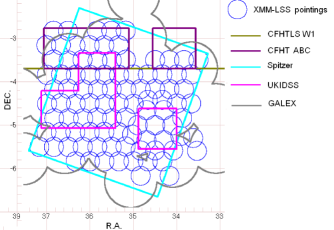
Figure 1: XMM-LSS field and multiwavelength coverage. CFHT ABC supplementary pointings are not the part of the Legacy Survey.

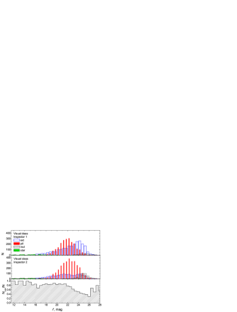
Figure 2: Magnitude distribution of 5142 visually classified objects by two independent inspectors (the top and middle panels). The fractional agreement between the two independent visual classifications is illustrated in the bottom panel.

3 Photo-z determination

For the photo-z determination we used the LePhare public code (Arnouts et al. 1999, Ilbert et al. 2006). First of all we compiled a training sample of objects with known spectroscopic redshifts. The spectroscopic redshifts for the XMM-LSS field sources were taken from the papers which are listed in the description of columns for Table 2. We only took into consideration those redshifts for which the angular separation between the optical counterpart of the X-ray source and the object observed spectroscopically is less than $1^{\prime\prime}$. We also visually verified that the coordinates associated to the spectra correspond to those of our optical counterparts. We found 783 spectroscopic redshifts for the optical counterparts, classified as galaxies and AGN/QSOs. We did not take into account 51 of the redshifts which have a rank ”3”, see the description of columns for Table 2. We have to note that an inhomogeneity of the spectroscopic data could affect the final accuracy of the photo-spectro-z relation but at this time we used all available information.

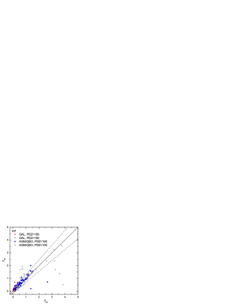
Figure 3: Photo-$z$ (7+ bands) vs. spectro-$z$ for the 243 visually classified extended objects (left panel) and the 479 $ptl$ objects (right panel). The solid lines correspond to $z_{ph}=z_{sp}$, the dashed lines correspond to $z_{ph}=z_{sp}\pm 0.15\times(1+z_{sp})$. PDZ represents the parameter appearing in the probability distribution of $z$ given by LePhare. PDF=100 means that the solution is unique.

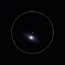
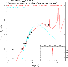
a	b	c	d
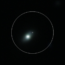
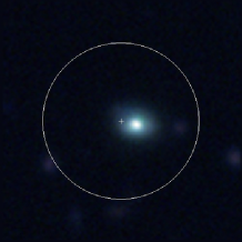
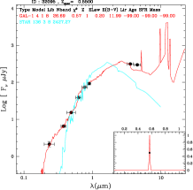
e	f	g	h

Figure 4: Examples of optical CFHTLS images and SEDs for selected objects from the $ext$ sample fitted with hybrid AGN contaminated templates. The color images are composed of the $g^{\prime}$, $i^{\prime}$ and $r^{\prime}$ band images. Below we list the spectro-$z$, the source of the spectral classification and estimated photo-$z$: $z_{sp}$=0.23 by Stalin et al. (2010) , $z_{ph}$=0.15 (a,b); $z_{sp}$=0.478 by Simpson et al. (2012), $z_{ph}$=0.496 (c,d); $z_{sp}$=0.205 by Garcet et al. (2007), $z_{ph}$=0.195 (e,f); $z_{sp}$=0.550 by Simpson et al. (2012), $z_{ph}$=0.569 (g,h). The radius of the white circle is 6^′′.

The photo-$z$ calculation was performed using 11 bands: $u^{*}$, $g^{\prime}$, $r^{\prime}$, $i^{\prime}$, $z^{\prime}$ (CFHTLS), $J$ and $K$ (UKIDSS), 3.6 and 4.5 $\mu$m (Swire/IRAC) and far-UV and near-UV bands of GALEX. As recommended by the authors of LePhare, we did not use bands above $\lambda>5\mu$m. Indeed, at those wavelength, the templates used for the Spectral Energy Distribution (SED) fitting are not reliable. For all the sources of the sample, we used the total magnitudes for all bands in the AB photometric system and took into account the Galactic extinction using $E(B-V)$ values according to the Schlegel (1998) maps and the Cardelli (1989) extinction law with $R_{v}$=3.1.

As described in Salvato et al (2011), we separately considered two samples of objects, according to our visual classification: extended, $ext$ (we assume that this sample mostly consists of galaxy dominated objects), and point-like, $ptl$ (AGN/QSO dominated sample). The photometric redshift calculation was performed using the Salvato et al. (2009) templates for our $ptl$ and $ext$ objects with $F_{(0.5-2keV)}>8\times 10^{-15}$ erg s^-1 cm^-2 and Ilbert et al. (2009) templates for the rest of the fainter X-ray objects following the flow-chart (Fig.8) by Salvato et al. (2011). The only differences are that we did not apply any variability correction and used the prior -30$<M_{abs}<$-22 for $ptl$. Extinction laws according to Calzetti et al. (2000) and Prevot et al. (1984) were applied to the Ilbert et al. (2009) normal galaxy templates as free fitting parameters. To the Salvato et al. (2009) templates we applied only the Prevot et al. (1984) extinction law. We computed the intrinsic galactic absorption $E(B-V)$ from 0.00 to 0.40 by steps of 0.05. For the redshift calculation we used a range from 0 to 6 with a step $\Delta z=0.01$, and at redshifts 6–7 with a step $\Delta z=0.05$. We added the emission lines to normal galaxy templates as in Ilbert et al. (2009).

We defined stars following the condition by Salvato et al. (2011): 1.5$\times\chi^{2}(STAR)<\chi^{2}(AGN/GAL)$, where $\chi^{2}(STAR)$ and $\chi^{2}(AGN/GAL)$ are the reduced $\chi^{2}$ for the best-fit solutions obtained with stellar and AGN or galaxy libraries. We found 183 stars, 83 from these were spectroscopically confirmed.

We estimated the photometric redshift accuracy using the measure $\sigma_{\Delta z/(1+z_{sp})}$, which according to Hoaglin et al. (1983) is given by:

$$\sigma_{\Delta z/(1+z_{sp})}=1.48\times\frac{{\rm median}|z_{ph}-z_{sp}|}{(1+z_{sp})}$$ (1)

The outliers are defined as those objects for which $|(z_{ph}-z_{sp})/(1+z_{sp})|>$0.15.

Table 1: Photometric redshift accuracy and fraction of the outliers for the samples of selected objects which have different numbers of photometric bands: 4 and more (4+), etc.

	$ext$			$ptl$			$all$
Sample	Ntot (Nsp)	$\sigma_{\Delta z/(1+z_{sp})}$	$\eta$,%	Ntot (Nsp)	$\sigma_{\Delta z/(1+z_{sp})}$	$\eta$,%	Ntot (Nsp)	$\sigma_{\Delta z/(1+z_{sp})}$	$\eta$,%
4+ bands	2234(259)	0.057	11.2	2201 (505)	0.091	27.6	4435 (764)	0.076	22.6
7+ bands	1330 (243)	0.057	10.4	1725 (500)	0.087	26.7	3055 (718)	0.074	21.8
9+ bands	415 (130)	0.057	7.7	570 (226)	0.074	22.1	985 (356)	0.063	16.9
7+ and PDZ=100	743 (195)	0.052	7.3	1072 (373)	0.074	23.9	1815 (568)	0.065	18.1
7+ and $i^{\prime}<$22	819 (209)	0.057	8.1	1278 (334)	0.076	25.0	2097 (635)	0.071	20.0

In Table 1 we show the values of the accuracy $\sigma_{\Delta z/(1+z_{sp})}$ and of the fraction of the outliers $\eta$ for the different samples of $ext$, $ptl$ and $all$=$ext$+$ptl$ objects as well as the numbers of objects in each sample. As expected the accuracy of photo-z for the $ext$ objects is much better than for $ptl$. As the sources are extended, they must be at a lower redshift and the galaxy component non negligible. It is well known that for normal galaxies the accuracy of photo-z is very high below redshift 1.5 also with few optical bands that are able to grasp the typical features of the SED ( i.e. the 4000 Å   break). On the contrary, point-like sources are at a higher redshift and the galaxy component is fainter than the power-law SED describing the bright nucleus. For these sources, intermediate band photometry would be necessary for identifying the emission lines and break the degeneracy among the possible redshift solutions (see Salvato et al 2009, Table 4). For example, for the $ext$ and $ptl$ samples of objects with 4 or more bands (4+) we have $\sigma_{\Delta z/(1+z_{sp})}$ = 0.057 and 0.091 with $\eta$ = 11.2 % and 27.6 %, respectively. Herewith for the $all$ sample $\sigma_{\Delta z/(1+z_{sp})}$ = 0.076 with $\eta$ = 22.6 %. We did not apply any magnitude cut to our samples but only 6% of our objects are fainter than $i^{\prime}$=24.5 and 0.4% are fainter than $i^{\prime}$=26.0 mag. We see that the accuracy of the photometric redshifts is increasing with the increasing number of bands.

In addition to the computation of the best photometric redshift solution, LePhare provides the redshift probability distribution (PDZ). For a large available number of bands the redshift solution appears as a clear peak with a PDZ near or equal to 100. When decreasing the number of bands and an increasing error in photometry, the PDZ presents either multi-peaks or a unique large distribution of possible solutions. We used the information in the PDZ for rejecting unreliable solutions, i.e. when two or more solutions for one object were produced. From Table 1 we see that if we consider objects with 7 and more (7+) bands with PDZ=100 then $\sigma_{\Delta z/(1+z_{sp})}$ and $\eta$ are practically the same as for the sample of objects having 9 or more (9+) bands. However in the case of 9+ bands the number of objects is twice less than in the case of 7+ bands with PDZ=100. In the last row of Table 1 we show the accuracy of photo-z for the magnitude-limited sample with $i^{\prime}<$22. We see that the accuracy of photo-z is only negligibly better than for the whole 7+ bands sample.

The relations between spectroscopic and photometric redshifts for the $ext$ and $ptl$ objects which have 7+ bands are presented in the left and right panels of Fig. 3, respectively. These samples have $\sigma_{\Delta z/(1+z_{sp})}$=0.057 and 0.087 with a fraction of outliers of 10.4% and 26.7%, respectively. The number of objects with PDZ$<100$ does not exceed 41% of the total number of objects. Meanwhile the number of outliers among these objects is only 34%.

We list hereafter some statistics: 85% of our $ext$ objects were fitted with normal galaxy templates (the rest with AGN/QSO hybrid templates) and 74% of $ptl$ were fitted with templates having an AGN/QSO contribution (the rest with normal galaxy templates). In Fig. 4 we show some Seyfert galaxies with clearly visible hosts and bright AGN. These objects are typical examples of X-ray sources which look like extended at optical wavelengths and have optical spectra and SEDs with an AGN/QSO contribution.

Table 2 presents a small fragment of data which is available through the Milan DB and the Centre de Données de Strasbourg (CDS) for all 5142 considered objects.

In this paper we considered the properties of only 3071 objects which have spectroscopic or photometric redshifts with rank 1 or 2 (see definitions in the description of columns for Table 2). Their redshift distribution is shown in the bottom panel of Fig. 5. The top panel of Fig. 5 presents the redshift distribution of 196 GALs and 2875 AGN/QSOs (the final classification is described in the next subsection). The median redshifts for the whole sample, GALs and AGN/QSOs are 1.20, 0.19, 1.27, respectively. We excluded from consideration 52 extended X-ray objects so they are not represented in Fig. 5.

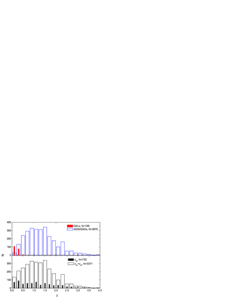
Figure 5: Lower Panel: Redshift distributions of all objects with known spectro-$z$ or photo-$z$ (white histogram) and of objects with spectro-$z$ (black histogram). Upper Panel: Redshift histogram of sources classified as GALs or AGN/QSOs from the z${}_{sp}+z_{ph}$ sample.

Table 2: List of an extracted sample of X-ray sources with optical counterparts and their redshifts: just as an example for several sources from the main catalog.

2XLSSd	Ora	Odec	zsp	zsprank	zspref	zspclass	zph	sedclass	zphrank	$HR$	$L_{Xsoft}$	$L_{Xhard}$	final_class	dogflag
(1)	(2)	(3)	(4)	(5)	(6)	(7)	(8)	(9)	(10)	(11)	(12)	(13)	(14)	(15)
J022006.8-045422	35.0288	-4.9060	null	null	null	null	0.92	gal	1	-1	3.0$\times 10^{42}$	null	AGN/QSO	0
J022008.7-045906	35.0364	-4.9849	1.65	1	4	AGN	1.55	agn/qso	1	-0.64	1.3$\times 10^{44}$	1.9$\times 10^{44}$	AGN/QSO	0
J022327.8-040119	35.8661	-4.0220	1.92	1	2	AGN	1.88	agn/qso	1	-0.62	2.9$\times 10^{44}$	3.4$\times 10^{44}$	AGN/QSO	0
J022500.4-040248	36.2523	-4.0466	0.61	2	5	GAL	1.95	agn/qso	3	-1	4.5$\times 10^{42}$	null	AGN/QSO	0
J022624.3-041343	36.6016	-4.2285	null	null	null	null	1.57	agn/qso	2	-1	1.3$\times 10^{44}$	null	AGN/QSO	1
J022630.7-040600	36.6274	-4.0998	0.00	1	4	STAR	0.00	star	3	-1	null	null	STAR	0
J022740.6-041857	36.9191	-4.3162	0.73	null	6	GAL	1.74	gal	2	-0.47	1.5$\times 10^{43}$	2.6$\times 10^{43}$	AGN/QSO	0
J022758.5-040851	36.9936	-4.1475	1.97	2	1	AGN	1.94	agn/qso	3	-1	8.2$\times 10^{43}$	null	AGN/QSO	0

(1) 2XLSSd name;
(2) RA of the optical counterpart;
(3) DEC of the optical counterpart;
(4) spectroscopic redshift when available;
(5) rank of the spectroscopic redshift: 1 - good quality (two or more lines in the spectra), 2 - acceptable redshifts (one clear line in the spectra) 3 - dubious redshift;
(6) source of the spectroscopic redshift: 1 – Le Fèvre et al. (2005) , 2 – Garcet et al. (2007), 3 – Lacy et al. (2007), 4 – Stalin et al. (2010), 5 – Lidman et al. (2012), 6 – the NASA/IPAC Extragalactic Database: http://nedwww.ipac.caltech.edu (NED), 7 – Simpson et al. (2006, 2012), 8 – Geach et al. (2007), 9 – Ouchi et al. (2008), 10 – Smail et al. (2008), 11 – van Breukelen et al. (2007,2009), 12 – Finoguenov et al. (2010), 13 – Akiyama et al. (2013); 14 – Croom et al. (2013). The compilation of redshifts from 7-14 can be found here: http://www.nottingham.ac.uk/ ppzoa/UDS_redshifts_18Oct2010.fits; 15 – SDSS DR9 data: www.sdss3.org. We did not use the SDSS redshifts in the calculations; they were added to the table later.
(7) spectral classification;
(8) photometric redshift;
(9) classification according to SED: GAL - normal galaxy templates of Ilbert et al. (2009) or templates #1-6 of Salvato et. al (2009), AGN/QSO - hybrid and AGN/QSO templates (#7-30) of Salvato et al. (2009);
(10) rank of the photometric redshift: 1 - good quality photometric redshift: 7 or more bands, $PDZ=100$; 2 - medium quality photometric redshift: 7 or more bands, PDZ$<100$; 3 - dubious photometric redshift, 4-6 bands; 4 - no redshift because of lack of photometry; 5 - no redshift because the objects are invisible (very faint) or wrong associations (probably misclassified);
(11) hardness ratio $HR$;
(12) X-ray luminosity in the soft band, erg/s;
(13) X-ray luminosity in the hard band, erg/s;
(14) final classification of the source;
(15) DOGs objects are flagged by 1 (see subsection 4.3 for the details).

4 X-ray and multiwavelength properties of selected objects

4.1 X-ray luminosity

Fig. 6 shows the X-ray luminosity of the sources, $L_{X}$, as a function of their redshift. The $K$-correction was applied to $L_{X}$ according to Burlon et al. (2011). We mark as ”GAL” all spectroscopically confirmed or photometrically classified galaxies (SEDs fitted by normal galaxy templates by Ilbert et al. 2009 or templates #1-6 by Salvato et al. 2009), except for sources with $L_{X,hard}>2\times 10^{42}$ erg/s (or $L_{X,soft}>10^{42}$ erg/s if the X-ray source was observed only in the soft band) which we consider AGN/QSOs as in Brusa et. al. (2010). We also refer to an object as AGN/QSO if it has a spectrum or a SED typical of an AGN or QSO. We have accordingly 196 (6.4%) GALs and 2875 (93.6%) AGN/QSOs that is in good correspondence with the COSMOS survey (6.3% of X-ray galaxies, Brusa et al. 2010). X-ray luminosities and final classification of all considered sources are noted in the last column of Table 2. We have to note that the final sample of GALs consists of 97% of visually classified $ext$ objects and 3% of $ptl$ while the final sample of AGN/QSOs consists of 39% and 61% of $ext$ and $ptl$, respectively.

Among the hard X-ray objects (those which have a flux in the 2-10 keV band) we selected a subsample of sources with X-ray to optical ratio X/O$>$10, as this characteristic indicator is important to identify highly obscured AGN/QSOs (see for example Fiore et al. 2003, Mignoli et al. 2004, Brusa et al. 2005, 2010). Our sample consists of 252 highly obscured AGN/QSO candidates which represents of 11% of the total AGN/QSO and 8% of the whole sample. In Fig. 7 we present the X-ray luminosity vs. $M_{i^{\prime}}$ absolute luminosity for GALs and AGN/QSOs, where the vertical solid lines $M_{i^{\prime}}$=-23.5 divide the AGN from the brighter QSOs. This limit is very close to the classical definition ($M_{B}$=-23). It is seen that the Hard ($HR\geq$-0.2) sources (filled symbols) are less bright than the Soft ($HR<$-0.2) ones.

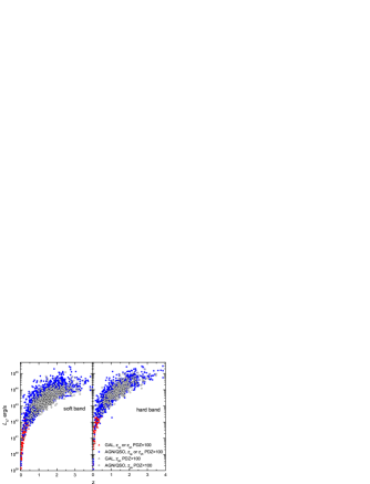
Figure 6: X-ray luminosity vs. redshift (photo and spectro) for the soft and hard bands.

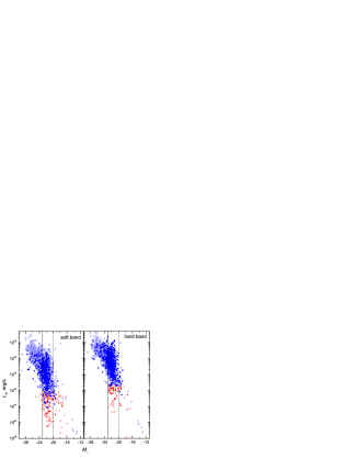
Figure 7: Dependence of X-ray luminosity vs. absolute magnitude in the $i^{\prime}$-band. GALs are marked with triangles, AGN with circles, while Soft ($HR<$-0.2) sources are shown with open and Hard ($HR\geq$-0.2) sources with filled symbols. The solid vertical lines $M_{i^{\prime}}$=-23.5 divide the AGN from the brighter QSOs. In the overdensity analysis (section 5) we have only considered the sources locating between the solid and dashed vertical lines.

4.2 The hardness ratio

The bottom panel of Fig. 8 presents the comparison of the XMM-LSS source distributions vs. their hardness ratio $HR=(H-S)/(H+S)$, where $S$ and $H$ denotes the count rate (cts/s) in the soft and the hard bands, respectively. Taking into account the average errors of the count rates measurements, we estimate a typical uncertainty for $HR$ of 0.1. We considered distributions of all the sources from the X-ray catalog, sources with optical counterparts and sources with spectro- or photo-z. We see that the various distributions look quite similar, so we do not see any distinction in the distributions between X-ray sources showing or not an optical counterpart: the Kolmogorov-Smirnov probability that distributions are the same is 0.92. The middle panel of Fig. 8 presents the distribution of $HR$ for the sources which were visually classified as extended $ext$ and point-like $ptl$. We may compare it with the upper panel where the distributions of $HR$ for GALs and AGN/QSOs are shown. We see that $ext$ sources show some excess of sources with $HR\geq$-0.2 in comparison with the $ptl$ sample.

The upper panel of Fig. 8 shows the distributions of $HR$ for GALs and AGN/QSOs. The samples of GAL and AGN/QSOs contain 62% and 45%, respectively, of the sources observed only in the soft band. The total source sample contains $\sim$46% of objects without a hard band detection, a fraction which is significantly larger than that of the COSMOS survey ($\sim$ 17%; Brusa et al. 2010). We see that some objects which appear as extended at optical wavelengths have a hard-spectrum and could be considered as candidates for obscured AGN. We plan to consider the properties of their host galaxies in a separate work.

The Kolmogorov-Smirnov probabilities that the $HR$ distributions are drawn from the same parent population for the pairs of samples $ext$ – $ptl$ and GAL – AGN/QSO are less than $10^{-10}$ and $10^{-5}$, respectively. The median $HR$ values in the corresponding quartile ranges for the All sources, AGN/QSOs and GALs are -0.63${}^{+0.34}_{-0.37}$, -0.60${}^{+0.32}_{-0.40}$ and -1${}^{+0.55}_{-0.00}$, respectively. Note, that 133 GALs out of the total of 196 were not observed in the hard band.

It is known that among sources with $HR\geq-0.2$ there are 80% of spectroscopically confirmed obscured QSOs (see for example Ghandi et al. 2004, Brusa et al. 2010 and references therein). We have 641 (21%) of objects with $HR\geq-0.2$ (606 of them are AGN/QSOs) while 154 of them (24%) also have X/O $>$10; these objects are faint at optical wavelengths and very bright in hard X-rays.

Figure 8: Distributions of the fractional number of XMM-LSS X-ray sources as a function of their hardness ratio: (i) for the cases of All X-ray sources, X-ray sources with optical counterparts, X-ray sources with spectro-$z$ or photo-$z$ (bottom panel); (ii) $ext$ and $ptl$ objects according to our visual classification (middle panel); (iii) GALs and AGN/QSOs according to spectroscopy, SEDs and/or L_X criteria (top panel).We plot Poisson uncertainties only in the upper panel for clarity.

4.3 Infrared colors

Lacy et al. (2004) proposed a useful approach for the classification of AGN with the help of a Spitzer/IRAC color-color diagram: with AGN/QSOs being concentrated within a compact region of such a diagram (see also Stern et al. 2005, Lacy et al. 2007, Brusa et al. 2009, 2010). In total 1467 (51%) AGN/QSOs and 117 GALs (60%) were observed in all 4 IRAC bands. The left panel of Fig. 9 presents the color-color plots for AGN/QSOs and GALs. We find that 1322 (91%) of AGN/QSOs and 19 (16%) of GALs are lying in the ”AGN region”.

Dey et al. (2008) and Brodwin et al. (2008) have proposed to select a population of high-redshift dust-obscured galaxies (DOGs) with large mid-infrared to ultraviolet luminosity ratios using simple criteria: $F_{24\mu m}\geq$ 0.3 mJy and $(R-[24])\geq$ 14 (Vega) mag, where $[24]\equiv$ -2.5 log${}_{10}(F_{24\mu m}$/7.29 Jy). Using these criteria, those authors found 2603 DOG candidates in the NOAO Deep Wide-Field Survey Bootes area, with 86 objects of their sample having $\langle z\rangle$=1.99 with $\sigma$=0.45. We have applied the Dey et al. (2008) criteria and found 54 DOG candidates which consist of 1.7% of our sample. Their average redshift is lower than that of Dey’s objects: $\langle z\rangle$=1.67 with $\sigma$=0.39. However this value is higher than that of the total sample $\langle z\rangle$=1.27 with $\sigma$=0.75 (see the $z$ distribution in Fig. 5). In the right panel of Fig. 9 we show the DOGs, hard objects with $HR\geq$-0.2 and objects with X/O$>$10. We see that the DOGs are concentrated in the upper corner of the ”AGN region”, while $HR\geq$-0.2 and obscured QSOs with X/O$>$10 are located in and near the ”AGN region”. Finally we note that out of the 154 $HR\geq-0.2$ and X/O$>10$ objects, 13 are DOGs. All DOGs are marked with ”1” in the last column of Table 2.

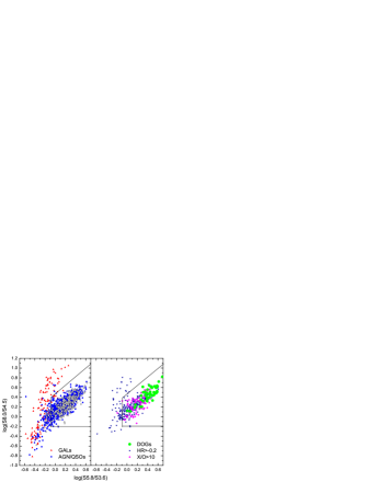
Figure 9: IRAC color-color plot. GALs and AGN/QSOs on the left panel (open symbols correspond to objects which have photo-$z$ with PDZ$<$100, as in Fig. 6). DOGs, HR$\geq$-0.2 and X/O$>$10 sources are shown on the right panel.

5 Environmental properties of the X-ray point-like sources

We wish to investigate the galaxy environment of our X-ray selected point-like sources. To this end we will use the CFHTLS W1 optical object catalog , but we will only consider ”galaxies” with star/galaxy classification index CLASS_STAR$<$0.95 and with the $i^{\prime}$-band limiting magnitude of 23.5, which is near to the catalog completeness limit . We have ignored the sources from the ABC fields (see Fig. 1) because these areas were not observed in the $i^{\prime}$-band. So the considered area in the environmental studies only concerns $\sim$9 sq. deg.

Taking into account the completeness limits of the CFHTLS and of our X-ray sample, we investigate the environment of X-ray sources in a volume limited region of their optical counterparts. This is defined by the redshift range 0.1$\leq z\leq$0.85 for which their optical counterparts are within the -23.5$<M_{i^{\prime}}\leq$-20 absolute magnitude range (while the rest-frame apparent magnitude of the knee of the $i^{\prime}$-band luminosity function has $m^{*}<$22.5; see Eq. 2). The luminosity limits can be seen in Fig. 7 on the $L_{X}$ vs. $M_{i^{\prime}}$ plots. We consider the following different subsamples of X-ray sources: All, GALs (only in the 0.1$\leq z\leq$0.55 redshift range) and AGN, Soft ($HR<$-0.2) and Hard ($HR\geq$-0.2) AGN. We expect that the overwhelming majority of our Soft AGN are unobscured AGN and the Hard AGN are obscured ones. In Fig. 10 we present the $M_{i^{\prime}}$ vs. $z$ distribution of All selected objects (N=777). We have to note that the accuracy of the photometric redshifts for this sample is $\sigma_{\Delta z/(1+z_{sp})}$=0.061 with $\eta$=13.8%. We did not reject from consideration the objects with PDZ$<$100 because the number of these objects in our low redshift sample does not exceed 17% (only 34% of objects with PDZ$<100$ are outliers). In any case, we repeated all calculations, excluding the dubious photo-$z$, and we reached the same conclusions.

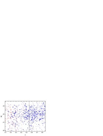
Figure 10: Diagram showing the absolute $i^{\prime}$-band magnitude versus redshift for our final volume limited All sample. GALs are marked with triangles, AGN with circles, while Soft ($HR<$-0.2) sources are shown with open and Hard ($HR\geq$-0.2) sources with filled symbols. The dashed line marks the separation between two chosen redshift ranges.

5.1 Overdensity measures

In order to calculate the optical galaxy overdensity around an X-ray source, we consider concentric annuli centered on each source (see an example in Fig.11). By taking into account their redshift and angular distance $D_{A}$, we estimate the linear sizes of the annuli at the source’s rest-frame distance. Then we count the number, $N_{i}$, of CFHTLS galaxies within a given annulus in the range of magnitudes from $m^{*}$ to $m^{*}+\Delta m$ (hereafter fainter galaxies) or from $m^{*}-\Delta m$ to $m^{*}$ (hereafter brighter galaxies), where $m^{*}$ is the apparent magnitude corresponding to the knee of the $i^{\prime}$-band luminosity function [$\Phi(L)$], given by:

$$m^{*}=5\log_{10}d_{L}+25+M_{i^{\prime}}^{*}+Q_{0.1}(z)+K_{0.1}(z)\;,$$ (2)

with $M_{i^{\prime}}^{*}(=-20.82+5\log_{10}h)$ the absolute magnitude of the knee of the $i$-band $\Phi(L)$ taken from Blanton et al. (2003b), $Q(z)$ and $K(z)$ the evolution and $K$-corrections, respectively, taken from Poggianti et al. (1997) and shifted to match their rest-frame shape at $z=0.1$, $d_{L}$ is the luminosity distance.

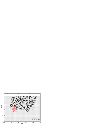
Figure 11: The CFHTLS W1 field and corresponding 777 XMM-LSS sources. An example of the annuli for one source is shown.

Next we have calculated the galaxy overdensities, $\delta_{i}$, within each annulus as:

$$\delta_{i}=\frac{N_{i}}{f_{i}N_{b}}-1\;,$$ (3)

where $N_{i}$ is the total number of objects within the $i^{th}$ radial annulus with surface area $A_{i}$, $N_{b}$ is the local background counts, estimated in the spherical annulus between 3.1 and 5 Mpc, with surface area $A_{b}$ and $f_{i}$ is the normalization factor that normalizes the background counts to the area of each spherical annulus. It is given by:

$$f_{i}=\frac{A_{i}}{A_{b}}\;.$$ (4)

Therefore, for each X-ray source we obtain the overdensity profile, $\delta_{i}(r)$, as a function of the source-centric distance $r$. The Poissonian uncertainty of the overdensity, $\delta_{i}$, is given by:

$$\sigma^{2}_{\delta_{i}}=\frac{1+\delta_{i}}{N_{b}}\left(\frac{1}{f_{i}}+1+\delta_{i}\right)$$ (5)

In order to have an estimate of the significance of the results, we compare the overdensity of galaxies around each of our sources with that expected in mock X-ray source distributions, having random coordinates but the same fiducial magnitude ($m^{*}$), estimated from the redshift of the X-ray source itself. For the mock, randomly distributed, sources we used the same CFHTLS optical catalog as we did for the real ones.

As an example, we find that the mean overdensity of the All sample within $0.1\leq z\leq 0.55$ and for the first radial annulus is $0.23\pm 0.80$ , while for the random distribution the corresponding value is $0.04\pm 0.75$. Clearly the apparent large scatter hinders our ability to distinguish environmental sample differences, based on the mean overdensity.

As a more sensitive alternative we use a Kolmogorov-Smirnov (KS) two-sample test in order to estimate quantitatively the differences between the real and random overdensity distributions, constructed for each radial distance annulus. In effect we use the cumulative overdensity distribution,

$$F(>\delta)=N(>\delta)/N_{tot}\;,$$

which is defined as the fraction of all sources ($N_{tot}$) having an overdensity above a given $\delta$. For the creation of the random overdensity distribution we have generated 100 random catalogs using the procedure described above. For each catalog we calculated the cumulative overdensity distribution $F(>\delta)$. Then we averaged these 100 distributions and obtained the final random distribution which we compared with the real one.

Fig. 12 shows the cumulative overdensity distributions for the real and mock samples, for the 0-0.4 Mpc and the 0.4-0.8 Mpc radial annuli, for the fainter ($m^{*}<m<m^{*}+1$) and brighter ($m^{*}-1<m<m^{*}$) galaxy environments and in the two $0.1\leq z\leq 0.55$ and $0.55<z\leq 0.85$ redshift ranges (see labels in each figure). Table 3 presents the corresponding KS probabilities (${\cal P}$) of the real and mock samples being drawn from the same parent population.

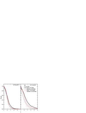
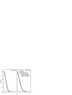
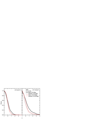
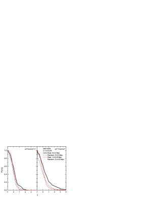
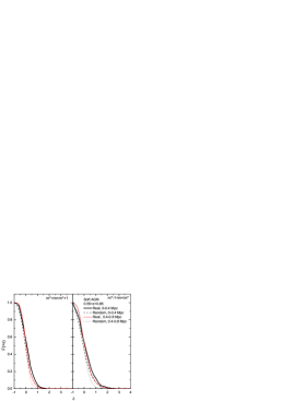
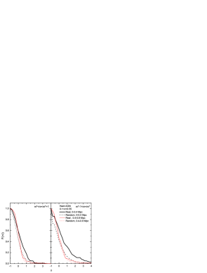
Figure 12: The cumulative distributions of overdensities for the real and mock samples, for the 0-0.4 Mpc and the 0.4-0.8 Mpc radial annuli, for the fainter m*$<$m$<$m*+1 and brighter m*-1$<$m$<$m* environments in the two $0.1\leq z\leq 0.55$ (left column) and $0.55<z\leq 0.85$ (right column) redshift ranges (see labels in each figure).

Table 3: The Kolmogorov-Smirnov probabilities (${\cal P}$) of the real and mock sample overdensity distributions (in the two indicated radial annuli) being drawn from the same parent population, for the fainter ($m^{*}<m<m^{*}+1$) and brighter ($m^{*}-1<m<m^{*}$) galaxy environments and in the two redshift ranges.

		$m^{*}<m<m^{*}+1$		$m^{*}-1<m<m^{*}$
Sample	N	${\cal P}_{0-0.4Mpc}$	${\cal P}_{0.4-0.8Mpc}$	${\cal P}_{0-0.4Mpc}$	${\cal P}_{0.4-0.8Mpc}$
0.1$\leq z\leq$0.55
All	375	3.7$\times 10^{-6}$	1.3$\times 10^{-5}$	1.9$\times 10^{-20}$	1.7$\times 10^{-8}$
GAL	105	3.4$\times 10^{-2}$	3.5$\times 10^{-1}$	1.8$\times 10^{-10}$	6.1$\times 10^{-1}$
AGN	270	4.7$\times 10^{-5}$	2.1$\times 10^{-3}$	8.7$\times 10^{-11}$	1.6$\times 10^{-4}$
Soft AGN	170	1.6$\times 10^{-3}$	9.3$\times 10^{-1}$	5.3$\times 10^{-7}$	6.2$\times 10^{-2}$
Hard AGN	100	5.0$\times 10^{-3}$	1.0$\times 10^{-1}$	1.9$\times 10^{-4}$	6.2$\times 10^{-1}$
0.55$<z\leq$0.85
All	402	7.6$\times 10^{-5}$	6.7$\times 10^{-5}$	1.7$\times 10^{-3}$	3.0$\times 10^{-4}$
Soft AGN	307	1.4$\times 10^{-4}$	4.2$\times 10^{-3}$	6.8$\times 10^{-3}$	3.8$\times 10^{-4}$
Hard AGN	95	2.6$\times 10^{-1}$	7.8$\times 10^{-1}$	4.5$\times 10^{-2}$	5.8$\times 10^{-1}$

Table 4: The fraction of sources having positive overdensity ($\delta>0$) for both the real and mock samples (in the two indicated radial annuli); for the fainter ($m^{*}<m<m^{*}+1$) and brighter ($m^{*}-1<m<m^{*}$) galaxy environments and in the two studied redshift ranges.

	$F(\delta>0)\pm\sigma^{*}$, %
	$m^{*}<m<m^{*}+1$		$m^{*}-1<m<m^{*}$
Sample	0-0.4 Mpc	0.4-0.8 Mpc	0-0.4 Mpc	0.4-0.8 Mpc
0.1$\leq z\leq$0.55
All	58$\pm$4	54$\pm$4	66$\pm$4	54$\pm$4
Allrand	45$\pm$3	46$\pm$4	41$\pm$3	44$\pm$3
GAL	55$\pm$7	52$\pm$7	72$\pm$8	52$\pm$7
GALrand	42$\pm$6	43$\pm$6	41$\pm$6	43$\pm$6
AGN	59$\pm$5	54$\pm$4	63$\pm$5	54$\pm$4
AGNrand	45$\pm$4	47$\pm$4	42$\pm$4	45$\pm$4
Soft AGN	59$\pm$6	49$\pm$5	64$\pm$6	49$\pm$5
Soft AGNrand	44$\pm$5	47$\pm$5	43$\pm$5	45$\pm$5
Hard AGN	59$\pm$8	57$\pm$8	63$\pm$8	57$\pm$8
Hard AGNrand	44$\pm$7	47$\pm$7	42$\pm$6	45$\pm$7
0.55$<z\leq$0.85
All	57$\pm$4	53$\pm$4	54$\pm$4	50$\pm$4
Allrand	46$\pm$3	47$\pm$3	45$\pm$3	47$\pm$3
Soft AGN	57$\pm$4	54$\pm$4	54$\pm$4	52$\pm$4
Soft AGNrand	46$\pm$4	48$\pm$4	45$\pm$4	47$\pm$4
Hard AGN	57$\pm$8	45$\pm$7	56$\pm$8	43$\pm$7
Hard AGNrand	47$\pm$7	46$\pm$7	44$\pm$7	46$\pm$7

^∗Here the uncertainty represents Poissonian noise.

Although our results show that X-ray point-like sources inhabit, both, dense and underdense environments, there are significantly more sources inhabiting overdense regions. In all samples we find that $F(\delta>0)\raise-3.0pt\hbox{\hbox to0.0pt{\hbox{$\sim$}\hss}\raise 4.0pt\hbox{$>$}\ }55\%$ for the first radial annuli (0-0.4 Mpc), with the random expectation being always $<45\%$ (Table 4). For example, for the case of the All sample, in the $0.1\leq z\leq 0.55$ redshift range and for the 0-0.4 Mpc radial annulus, we find that the fraction of sources with positive overdensity, $F(\delta>0)$, is 58$\pm$4%/66$\pm$4% for the fainter/brighter environments, while the corresponding random expectation is 45%/41%, respectively (see Table 4 and left top panel in Fig.12).

Furthermore, the KS test show significant differences between the All source overdensity distribution and their random expectations, for both fainter and brighter environments, and for the two first radial annuli (see Table 3). In the third radial annulus (0.8-1.2 Mpc), the probability of an overdensity distribution difference, with respect to the random case, drops to levels ranging from $\sim 0.05$ to 0.3 for both type of environments and redshift ranges, and we conclude that at such large scales we cannot identify significant environmental differences with respect to the random expectations. Subtle differences could possibly be revealed only with the use of full redshift information of the surrounding galaxies.

An important result of our analysis is that for all our samples the overdensities in the 0.1$\leq z\leq$0.55 redshift range are larger and more significant than those in the $0.55<z\leq 0.85$ range. For example, the fraction of All X-ray sources having positive overdensities of brighter galaxies in the 0-0.4 Mpc annulus, increases from 54$\pm$4% to 66$\pm$4%, between the higher and lower $z$-ranges. This effect is clearly seen by inspecting Table 3 and Fig.13 (upper panel), where we present the ratio of the galaxy overdensity distributions between the lower and higher redshift ranges studied for the All sample. In the lower panel of Fig.13 we present the corresponding ratio separately for the Soft and Hard AGN sources, which also show a positive evolution of their galaxy overdensities. A more relevant discussion will be presented further below.

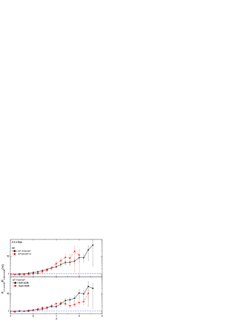
Figure 13: The ratio of the galaxy overdensity distributions between the lower and higher redshift ranges studied (only in the 0-0.4 Mpc radial annulus). Errorbars correspond to Poissonian uncertainties. Upper Panel: the All sample. Lower Panel: the Hard and Soft AGN samples (only the brighter environment).

Therefore, there is a positive redshift evolution of the galaxy overdensity amplitude and/or significance, within which X-ray sources are embedded. A similar (weak) tendency was reported by Strand et al. (2008) for the environments of the optically selected type I quasars.

Again inspecting Table 4 and Fig.12 we have another, generic, result valid for all the considered samples, which is that the overdensities defined by the brighter galaxies are typically larger and more significant than those defined by fainter galaxies. This result should be related to the well known correlation between galaxy luminosity and clustering amplitude (see for example Zehavi et al. 2005, McCracken et al. 2007, Guo et al. 2013 and references therein).

Furthermore, we can reach a number of interesting conclusions regarding the environmental differences between the different source types (AGN, GAL, Soft and Hard AGN).

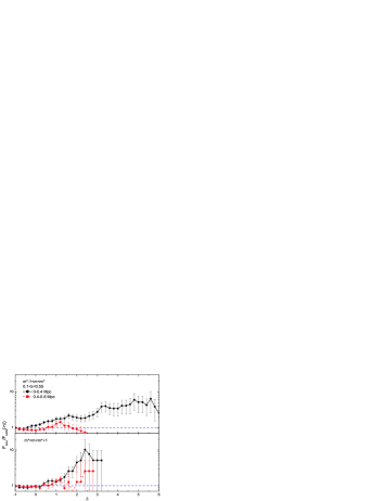
Figure 14: The ratio of the overdensity distributions of the GAL and AGN samples for both fainter (lower panel) and brighter (upper panel) environments. Black and red curves correspond to the 0-0.4 Mpc and 0.4-0.8 Mpc annuli, respectively.

For example, X-ray galaxies (GAL sample) are found in significantly larger galaxy overdensities with respect to AGN. This can be clearly seen in Fig.14 where we plot the ratio of the overdensity distributions of the GAL and AGN samples. The excess, by large factors ($\sim 2-10$), of the positive galaxy overdensities around GAL sources, with respect to those around AGNs, can be clearly seen but only in the 0-0.4 Mpc annulus (black line) for both fainter and brighter environments. For the latter type of environment we have that $F(\delta>0)$=72$\pm$8% (with random expectation 41%) and $F(\delta>1)$=45$\pm$7%, when for comparison, the corresponding values for the AGN sample is $F(\delta>0)$=63$\pm$5% (with random expectation 43%) and $F(\delta>1)$=26$\pm$3%, respectively.

Another interesting, but somewhat unexpected within the unification paradigm, result is that the Soft and Hard AGN samples show significant galaxy overdensity distribution differences. Inspecting Fig.15, where we plot the ratio of the overdensity distributions of the Hard and Soft AGN samples, for those cases where both overdensity distributions are significantly different than their random expectations, we see that the Hard AGN sample has always (for $\delta\raise-3.0pt\hbox{\hbox to0.0pt{\hbox{$\sim$}\hss}\raise 4.0pt\hbox{$>$}\ }0$) a larger fraction of higher galaxy overdensity values with respect to the Soft AGN’s (i.e., $F_{\rm Hard}/F_{\rm Soft}(\delta)>1$). This is apparent in both redshift ranges, although in the higher-$z$ range it appears to be more significant. This result is in general agreement with the correlation function analysis of the XMM-LSS sources by Elyiv et al. (2012), where the clustering of the Hard AGNs was found to be stronger than that of the Soft AGNs.

Finally, we find another interesting result which is the different redshift evolution of the galaxy overdensity distribution for the Soft and Hard sources. In the lower panel of Fig.13 we plot the ratio of the overdensity distributions between the lower and higher redshift ranges, separately for the Soft (continuous black line) and Hard (red dashed line) AGN in the 0-0.4 Mpc radial annulus. There are indication of a systematic difference by which the galaxy overdensities (for $\delta\raise-3.0pt\hbox{\hbox to0.0pt{\hbox{$\sim$}\hss}\raise 4.0pt\hbox{$>$}\ }1.5$) within which the Hard AGN are embedded evolve less rapidly than the corresponding overdensities around Soft AGN.

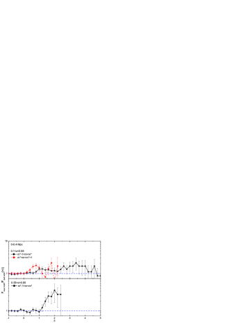
Figure 15: The ratio of the galaxy overdensity distributions of the Hard and Soft AGN samples for the 0-0.4 Mpc radial annulus, for the fainter (red dashed line) and brighter (black continuous line) environments. Upper/Lower panels correspond to the lower/higher $z$-range studied.

5.2 Nearest neighbour statistics

We attempted to investigate the very close environment around each X-ray source by using a nearest neighbour analysis. To this end we estimated for each X-ray source the rest-frame projected linear distance to its nearest optical neighbour (NNb) using the same CFHTLS galaxy catalog, as in the overdensity analysis, but within the magnitude ranges $m_{i^{\prime}}$+$\Delta m$ with $\Delta m=\pm$ 0.5 or $\pm$1, where $m_{i^{\prime}}$ is the $i^{\prime}$-band magnitude of the host galaxy of the X-ray source. Note, that contrary to the overdensity analysis for which the characteristic magnitude, $m^{*}$, used to define the fainter and brighter environment around our X-ray sources, was that corresponding to the knee of the $i$-band luminosity function, in the current analysis the characteristic magnitude, $m_{i^{\prime}}$, is that of the host galaxy.

We have then compared, using the KS two-sampled test, the NNb distance distribution of our X-ray sources with that of randomly selected CFHTLS galaxies having a similar magnitude with that of the X-ray source host ($\left|m_{i^{\prime},X-ray}-m_{i^{\prime},rand}\right|<0.1$), and found no significant difference whatsoever. In Table 5 we present the KS probabilities of the indicated pairs of NNb distributions, for $\Delta m=+1.0$, -1.0, +0.5, -0.5, being drawn from the same parent population.

It is evident that the only pair of NNb sample distributions that show a deviation which is marginally significant (${\cal P}_{KS}\simeq 0.01$) is that of the GAL and AGN brighter neighbors ($\Delta m$=-1.0 and -0.5). Inspecting the two distributions (Fig. 16) we see that the difference is attributed to a deficiency of GAL neighbours at a distance of $\sim 0.2$ Mpc and a corresponding excess at $\sim 0.7$ Mpc, and not to an overall difference in the shape of the distributions. We consider that the observed difference is not very significant and do not discuss it further.

We have also tested the corresponding 5^th nearest neighbour distributions and the results remain the same.

We conclude that the NNb analysis, applied on our projected data, cannot be effectively used to characterize differences in the very close environment of different types of X-ray sources.

Table 5: The Kolmogorov-Smirnov probability of the indicated pairs of NNb distributions being drawn from the same parent population and for the indicated magnitude range.

	${\cal P}_{KS}$
Sample 1/Sample 2	$\Delta m=+1$	$\Delta m=-1$	$\Delta m=0.5$	$\Delta m=-0.5$
$0.1\leq z\leq 0.55$
All/Allrand	0.65	0.77	0.98	0.65
GAL/AGN	0.73	0.01	0.55	0.01
Soft AGN/Hard AGN	0.99	0.35	0.55	0.91
$0.55<z\leq 0.85$
All/Allrand	0.99	0.73	0.98	0.99
Soft AGN/Hard AGN	0.97	0.99	0.25	0.98

Figure 16: Differential distributions of the nearest neighbour distance for the sample of GALs and AGN for two different magnitude ranges in the $0.1\leq z\leq 0.55$ redshift range.

6 Summary and main conclusions

In this paper we have classified 5142 XMM-LSS X-ray selected sources. In order to check their reliability and positions, reject ”problematic” objects (i.e. defects in the observations, doubtful counterparts, etc.) and finally classify each object, we visually inspected the optical images of all X-ray counterparts in the $g^{\prime}$, $i^{\prime}$ and $r^{\prime}$ CFHTLS bands. We classified 2441 objects as being extended and 2280 as being point-like, while we rejected from consideration 238 ”problematic” objects and 183 stars (5% and 4% of the whole sample, respectively). We estimated the photometric redshifts of the 4435 objects for which there is available photometry in 4-11 bands [i.e., CFHTLS, Spitzer/IRAC, UKIDSS and GALEX], $i^{\prime}<$26 mag. Furthermore, 783 objects also have spectroscopic redshifts. We have found that the photometric redshift accuracy for the objects with available 4-11 band photometry is $\sigma_{\Delta z/(1+z_{sp})}$=0.076 with $\eta$=22.6% of outliers. The corresponding values for the objects with 7-11 bands are $\sigma_{\Delta z/(1+z_{sp})}$=0.074 with $\eta$=21.8% and for the subsample of objects with PDZ=100: $\sigma_{\Delta z/(1+z_{sp})}$=0.065 with $\eta$=18.1%.

We have considered the multiwavelength properties of 3071 objects which have spectroscopic redshifts or photometric redshifts calculated from 7-11 bands. According to our classification, based on spectra, SEDs and/or $L_{X}$, we have 196 (6.4%) GALs and 2875 (93.6%) AGN/QSOs in our sample. The median $HR$ values in the corresponding quartile ranges for the All sources, AGN/QSOs and GALs are -0.63${}^{+0.34}_{-0.37}$, -0.60${}^{+0.32}_{-0.40}$ and -1${}^{+0.55}_{-0.00}$, respectively. We have also found that 252 objects (8% of our sample) have X/O$>$10 and 641 (21%) have $HR\geq$-0.2, which makes them good candidates for obscured AGN/QSOs. We have found 54 DOG candidates (1.7%) in our sample.

We have then defined the environment of 777 X-ray sources (GALs, Soft and Hard AGN ($HR<$-0.2 and $HR\geq$-0.2, respectively) which we considered as unobscured and obscured ones) with -23.5$<M_{i^{\prime}}<$-20 in the 0.1$\leq z\leq$0.85 redshift range. The photo-z accuracy for this low redshift sample is $\sigma_{\Delta z/(1+z_{sp})}$=0.061 with $\eta$=13.8% outliers. Two types of environments have been defined for each X-ray source; an overdensity of fainter and of brighter galaxies (by one magnitude) with respect to the rest-frame magnitude of the knee of the $i^{\prime}$-band luminosity function. Our main results are the following:

(1) The X-ray point-like sources typically reside in overdense regions, although they can be found even in underdense regions. We find that $\sim$$>$ 55-60% of all X-ray sources are located in overdense environments ($\delta>$0), a result which is significantly higher than the random expectation.

(2) Overdensities around X-ray sources defined by bright neighbours are significantly larger than those defined by faint neighbours. For the first redshift range $0.1\leq z\leq 0.55$ the percentage of objects with positive overdensity having fainter and brighter environments are 58$\pm$4% and 66$\pm$4% against 45% and 41% expected for the random distribution of the sources, respectively.

(3) Overdensities around X-ray sources, defined either by brighter or fainter neighbours, are typically larger and more significant in the $0.1\leq z\leq 0.55$ rather than in the $0.55<z\leq 0.85$ redshift range. Therefore there appears to be a positive redshift evolution of the galaxy overdensity amplitude within which X-ray sources are embedded.

(4) X-ray galaxies and AGN inhabit different environments. X-ray selected galaxies inhabit significantly more overdense brighter galaxy regions with respect to AGN, indicating possibly that the former prefer more cluster-like environments, while the latter group-like ones. However, the overdensities around X-ray galaxies are significant only up to $\sim 0.4$ Mpc, while those around AGN up to $\sim 0.8$ Mpc. Our results are in general agreement with Georgakakis et al. (2007, 2008), who showed that X-ray-selected AGN, at $z\sim$1, prefer to reside in groups and with Bradshaw et al. (2011) who found that X-ray AGN, in the UDS (SXDS) field with 1.0$<z<$1.5, inhabit significantly overdense environments corresponding to dark matter haloes of $M\raise-3.0pt\hbox{\hbox to0.0pt{\hbox{$\sim$}\hss}\raise 4.0pt\hbox{$>$}\ }10^{13}M_{\odot}$.

(5) The obscured AGN ($HR\geq-0.2$) are located in more overdense regions with respect to the unobscured AGN ($HR<-0.2$). This is true for both brighter and fainter galaxy environments in the 0.1$\leq z\leq$0.55 redshift range, while it is evident only for the brighter environment in the $0.55<z\leq 0.85$ range. This result is in general agreement with the correlation function analysis of the XMM-LSS X-ray point-source catalog (having a median $z\sim 1$), presented in Elyiv et al. (2012), where the clustering of the Hard AGN was found to be stronger than that of the Soft AGN. Hickox et al. (2012) also found a stronger clustering of obscured QSOs with respect to than of unobscured ones in the 0.7$<z<$1.8 redshift range in the Bootes multiwavelength survey, although Allevato et al. (2011) found an opposite trend.

(6) There are some indication that unobscured AGN ($HR<-0.2$) have a more rapid evolution of their galaxy overdensity amplitude, $\delta$, between the two redshift ranges studied, with respect to the obscured AGN ($HR\geq-0.2$).

- (1) Akiyama, M. et al. 2013 (in preparation)
- (2) Allevato, V., Finoguenov, A., Cappelluti, N., et al. 2011, ApJ, 736, id. 99
- (3) Antonucci, R. 1993, Ann. Rev. Astron. & Astrophys., 31, 473
- (4) Arnouts, S., Cristiani, S., Moscardini, L., et al. 1999, MNRAS, 310, 540
- (5) Blanton, M. R., Hogg, D. W., Bahcall, N. A., et al. 2003a, ApJ, 594, 186
- (6) Blanton, M. R., Hogg, D. W., Bahcall, N. A., et al. 2003b, ApJ, 592, 819
- (7) Bradshaw, E. J., Almaini, O., Hartley, W. G., et al., 2011, MNRAS, 415, 2626
- (8) Brusa, M., Comastri A., Daddi, E., et al. 2005, A&A, 432, 69
- (9) Brusa, M., Fiore, F., Santini, P. et al. 2009, A&A, 507, 1277
- (10) Brusa, M., Civano, F., Comastri, A., et al. 2010, ApJ, 716, 348
- (11) Brodwin, M., Dey, A., Brown, M. J. I., et al. 2008, ApJ, 687, L65
- (12) Burlon, D., Ajello M., Greiner, J. et al. 2011, ApJ, 728, 58
- (13) Calzetti, D., Armus, L., Bohlin, R., C., et al. 2000, ApJ, 533,682
- (14) Cardelli, J. A., Clayton, G. C., Mathis, J. S. 1989, ApJ, 345, 245
- (15) Chiappetti, L., Tajer, M., Trinchieri, G. et al. 2005, A&A, 439, 413
- (16) Chiappetti, L., Clerc, N., Pacaud, F., et al. 2012 submitted to MNRAS
- (17) Constantin, A., Hoyle, F., Vogeley, M. S., 2008, ApJ, 673, 715
- (18) Croom et al. (2013) in prep.
- (19) Dey, A., Soifer, B. T., Desai, V., et al. 2008, ApJ, 677, 943
- (20) Dressler, A. 1980, ApJ, 236, 361
- (21) Downes, A.J.B., Peacock, J.A., Savage, A., et al. 1986, MNRAS, 218, 31
- (22) Elyiv, A., Clerc, N., Plionis, M. 2012, A&A, 537, id.A131
- (23) Falder, J. T., Stevens, J. A., Jarvis, M. J., et al. 2010, MNRAS, 405, 347
- (24) Fanidakis, N., Baugh, C. M., Benson, A. J. et al. 2012, MNRAS, 419, 2797
- (25) Fiore, F., Brusa, M., Cocchia, F., et al. 2003, A&A, 409, 79
- (26) Finoguenov, A., Watson, M. G., Tanaka, M. et al. 2010, MNRAS, 403, 2063
- (27) Gandhi, P., Crawford, C. S., Fabian, A. C., Johnstone, R. M. 2004, MNRAS, 348, 529
- (28) Gandhi, P., Garcet, O., Disseau, L. et al. 2006, A&A, 457, 393
- (29) Garcet, O., Gandhi, P., Gosset, E. et al. 2007, A&A, 474, 473
- (30) Geach, J.E., Simpson, C., Rawlings, S., Read, A. M., Watson, M. 2007, MNRAS, 381, 1369
- (31) Georgakakis, A., Nandra, K., Laird, E. S., et al. 2007, ApJ, 660, L15
- (32) Georgakakis, A., Gerke, B. F., Nandra, K., et al. 2008, MNRAS, 391, 183
- (33) Gilmour, R., Gray, M. E., Almaini, O. et al. 2007, MNRAS, 380, 1467
- Guo et al. (2013) Guo, H., Zehavi, I., Zheng, Z., et al. 2013, ApJ, 767, 122
- (35) Hickox, C., Myers, A. D., Brodwin, M. et al. 2011, ApJ, 731, 117
- (36) Hoaglin, D. C., Mosteller, F., Tukey, J.W. 1983, in Understanding Robust and Exploratory Data Analysis (Wiley Series in Probability and Mathematical Statistics), ed. D. C. Hoaglin, F.Mosteller, & J.W. Tukey (New York:Wiley)
- (37) Ilbert, O., Arnouts, S., McCracken, H. J., et al. 2006, A&A, 457, 841
- (38) Ilbert, O., Capak, P., Salvato, M. et al. 2009, ApJ, 690, 1236
- (39) Kauffmann, G., White, S. D. M., Heckman, T. M. 2004, MNRAS, 353, 713
- (40) Koulouridis, E., Plionis, M., Chavushyan, V., Dultzin-Hacyan, D., Krongold, Y., Goudis, C., 2006, ApJ, 639,3745
- (41) Koutoulidis, L., Plionis, M., Georgantopoulos, I., Fanidakis, N., 2012, MNRAS in press (arXiv/1209.6460)
- (42) Lacy, M., Storrie-Lombardi, L. J., Sajina, A., et al. 2004, ApJ Suppl. Ser., 154, 166
- (43) Lacy, M., Petric, A. O., Sajina, A., et al. 2007, AJ, 133, 186
- (44) Le Fèvre, O., Vettolani, G., Garilli, B., et al. 2005, A&A 439, 845
- (45) Li, C., Kauffmann, G., Wang, L. 2006, MNRAS, 373, 457
- (46) Lietzen, H., Heinamaki, P., Nurmi, P., et al. 2009, A&A, 501, 145
- (47) Lietzen, H., Heinamaki, P., Nurmi, P., et al. 2011, A&A, 535, id.A21
- (48) Lidman, C., Ruhlmann-Kleider, V., Sullivan, M., et al. 2012 accepted in PASA
- (49) Lupton, R. H., Juric, M., Ivezic, Z., et al. 2005, Bull. AAS, 37, 1384
- McCracken et al. (2007) McCracken, H. J., Peacock, J. A., Guzzo, L., et al. 2007, ApJS, 172, 314
- (51) Mignoli, M., Pozzetti, L., Comastri, A., et al. 2004, A&A, 418, 827
- (52) Miyaji, T., Krumpe, M., Coil, A. L. Aceves, H. 2011, ApJ, 726, id. 83
- (53) Montero-Dorta, A. D., Croton, D. J., Renbin, Y., et al. 2009, MNRAS, 392, 125
- (54) Nakos, T., Willis J. P., Andreon, S., et al. 2009, A&A, 494, 579
- (55) Ouchi, M., Shimasaku, K., Akiyama, M., et al. 2008, ApJ. Suppl. Ser., 176, 301
- (56) Pierre, M., Chiappetti, L., Pacaud, F., et al. 2007, MNRAS, 382, 279
- (57) Poggianti, B. 1997, A & A Suppl. Ser., 122, 399
- (58) Polletta, M., Tajer, M., Maraschi, L., et al. 2007, ApJ, 663, 81
- (59) Prevot, M. L., Lequeux, J., Prevot, L. et al. 1984, A&A, 132, 389
- (60) Schawinski, K., Virani, S., Simmons, B., et al. 2009, ApJ, 692, L19
- (61) Schlegel, D. J., Finkbeiner, D. P., Davis, M. 1998, ApJ, 500, 525
- (62) Salvato, M., Hasinger, G., Ilbert, O., et al. 2009, ApJ, 690, 1250
- (63) Salvato, M., Ilbert, O., Hasinger, G., et al. 2011, ApJ, 742, id. 61
- (64) Silverman, J. D., Kovac, K., Knobel, C., et al. 2009, ApJ, 695, 171
- (65) Simpson, C., Martinez-Sansigre A., Rawlings, S., et al. 2006, MNRAS, 372, 741
- (66) Simpson, C., Rawlings, S., Ivison, R., et al. 2012, MNRAS, 421, 2012
- (67) Smail, I., Sharp R., Swinbank, A. M., et al. 2008, MNRAS, 389, 407
- (68) Sorrentino, G., Radovich, M., Rifatto, A. 2006, A&A, 451, 809
- (69) Stalin, C.S., Petitjean, P., Srianand, R., et al. 2010, MNRAS, 401, 294
- (70) Stern, D., Eisenhardt, P., Gorjian, V., et al. 2005, ApJ, 631, 163
- (71) Strand, N. E., Brunner, R. J., Myers, A. D., 2008, ApJ, 688, 180
- (72) Tajer, M., Polletta, M., Chiappetti, L., et al. 2007, A&A, 467, 73
- (73) Tasse, C., Le Borgne, D., Rottgering, H., et al. 2008a, A&A 490, 879
- (74) Tasse, C., Best, P.N., Rottgering, H., Le Borgne, D. 2008b, A&A, 490, 893
- (75) Tasse, C., Rottgering, H., Best P.N. 2011, A&A, 525, 127
- (76) van Breukelen, C., Cotter, G., Rawlings, S., et al. 2007, MNRAS, 382, 971
- (77) van Breukelen, C., Simpson, C., Rawlings, S., et al. 2009, MNRAS, 395, 11
- (78) van der Wel, A. 2008, ApJ, 675, L13
- (79) Warren, S. J., Hewett, P. C., Osmer P. S. 1994, ApJ, 421, 412
- (80) Waskett ,T.J., Eales, S.A., Gear, W.K., et al. 2005, MNRAS, 363, 801
- (81) Ueda, Y., Watson, M.G., Stewart, I.M., et al. 2008, ApJ Suppl. Ser., 179, 124
- Zehavi et al. (2005) Zehavi, I., Zheng, Z., Weinberg, D. H., et al. 2005, ApJ, 630, 1