Dynamics of a spherical object of uniform density
in an expanding universe

Abstract

We present Newtonian and fully general-relativistic solutions for the evolution of a spherical region of uniform interior density $\rho_{\rm i}(t)$, embedded in a background of uniform exterior density $\rho_{\rm e}(t)$. In both regions, the fluid is assumed to support pressure. In general, the expansion rates of the two regions, expressed in terms of interior and exterior Hubble parameters $H_{\rm i}(t)$ and $H_{\rm e}(t)$, respectively, are independent. We consider in detail two special cases: an object with a static boundary, $H_{\rm i}(t)=0$; and an object whose internal Hubble parameter matches that of the background, $H_{\rm i}(t)=H_{\rm e}(t)$. In the latter case, we also obtain fully general-relativistic expressions for the force required to keep a test particle at rest inside the object, and that required to keep a test particle on the moving boundary. We also derive a generalised form of the Oppenheimer–Volkov equation, valid for general time-dependent spherically-symmetric systems, which may be of interest in its own right.

I Introduction

In a recent paper, we presented metrics for a point mass residing in each of a spatially-flat, open and closed expanding universe Nandra et al. (2012). These were derived using a tetrad-based procedure in general relativity Lasenby et al. (1998), and are essentially a combination of the Schwarzschild metric and the Friedmann–Robertson–Walker (FRW) metric for a homogeneous and isotropic universe. In particular, we used our metrics to study particle dynamics outside the central object. As one might expect intuitively, for radial motion in the Newtonian limit, the force acting on a test particle was found in all three cases to comprise of the usual $1/r^{2}$ inwards component due to the central mass and a cosmological component proportional to $r$ that is directed outwards (inwards) when the expansion of the universe is accelerating (decelerating).

A natural progression of this work is to consider a central object of finite spatial extent. It may initially seem sensible (as it did to other authors) to proceed by deriving an interior metric that, at the boundary of the object, matches onto a previously obtained exterior solution for the case of a central point mass. In fact, this approach is too restrictive, since the interior model has to be set up so that the effects of the object’s own expansion vanish at its boundary. We therefore consider the problem afresh and model the physical system in the manner illustrated in Fig. 1. Indeed, this figure may be taken as the definition of our model, in which a spherical massive object of size $a(t)$ and uniform interior density $\rho_{\rm i}(t)$ resides in an expanding universe with uniform exterior density $\rho_{\rm e}(t)$. In general, the spatially-uniform ‘Hubble parameters’ of the interior and exterior regions are independent, and denoted by $H_{\rm i}(t)$ and $H_{\rm e}(t)$ respectively.

From the figure, we may write down an expression for the total mass (or energy in the relativistic case; will use natural units $c=G=1$ throughout) contained within a sphere of physical radius $r$. We denote this by $M(r,t)$, but note that dependencies on $r$ and $t$ will usually be suppressed in the equations below, whereas those on $r$ or $t$ alone will usually be made explicit. It is clear that

$$M=\begin{cases}\frac{4}{3}\pi\rho_{\rm i}(t)r^{3},&\text{$r\leq a(t)$},\\ \frac{4}{3}\pi\rho_{\rm e}(t)(r^{3}-a^{3}(t))+\frac{4}{3}\pi\rho_{\rm i}(t)a^{3}(t),&\text{$r>a(t)$}.\end{cases}$$

We may rewrite the second of these cases and work with the alternative expressions

$$M=\begin{cases}\frac{4}{3}\pi\rho_{\rm i}(t)r^{3},&\text{$r\leq a(t)$},\\ \frac{4}{3}\pi\rho_{\rm e}(t)r^{3}+m(t),&\text{$r>a(t)$},\end{cases}$$ (1)

where $m(t)=\frac{4}{3}\pi(\rho_{\rm i}(t)-\rho_{\rm e}(t))a^{3}(t)$ is the mass contained within the boundary $a(t)$ at time $t$, in excess of that which would be present due to the background alone.

As will we show, in both the Newtonian and fully general-relativistic cases, the dynamical evolution of the system may be determined completely by specifying the internal and external Hubble parameters $H_{\rm i}(t)$ and $H_{\rm e}(t)$, respectively (together with the radius $a_{\ast}\equiv a(t_{\ast})$ and density $\rho_{\ast}\equiv\rho_{\rm i}(t_{\ast})$ of the object at some reference time $t=t_{\ast}$). Typically, we will take $H_{\rm e}(t)$ to correspond to some expanding exterior universe of interest, but $H_{\rm i}(t)$ can, in principle, have any form (and be positive or negative). This follows from allowing the relationship between the fluid pressure and density to be arbitrary, since then the interplay between the internal pressure of the object and its self-gravity may allow it to expand or contract at any rate. This freedom would disappear, however, if one imposed an equation of state.

We note that, following our approach in Nandra et al. (2012), in each region (interior and exterior) we assume a single ‘phenomenological’ fluid. This avoids the complexity of an explicit multi-fluid treatment, whereby one would separate the fluid in each region into its baryonic and dark matter components.

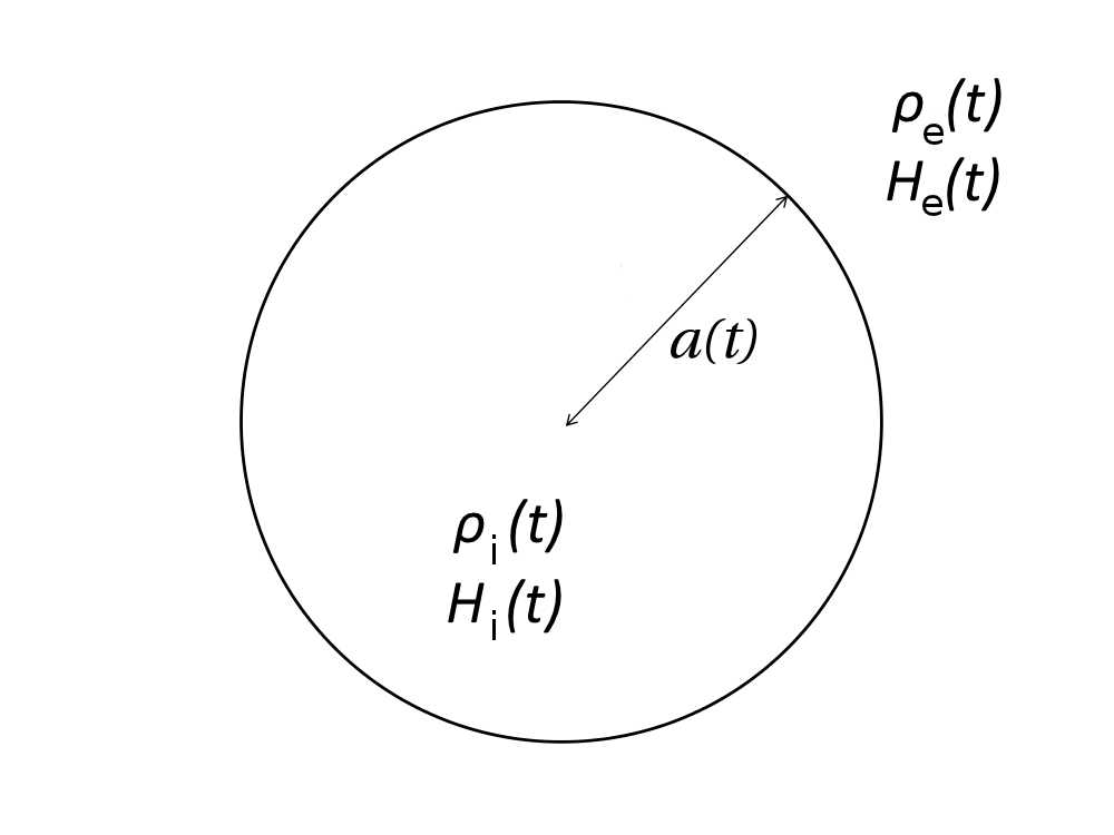
Figure 1: Model of a spherical object of size $a(t)$ and uniform interior density $\rho_{\rm i}(t)$ residing in an expanding universe with uniform exterior density $\rho_{\rm e}(t)$. The corresponding ‘Hubble parameters’ of the interior and exterior regions are denoted $H_{\rm i}(t)$ and $H_{\rm e}(t)$, respectively.

In particular, in each region we assume a single overall (uniform) fluid density and a single associated (effective) pressure. It is envisaged that the pressure comprises the ordinary gas pressure due to baryonic matter, and an effective pressure from the dark matter that arises from the motions of dark matter particles having undergone phase-mixing and relaxation (see Lynden-Bell (1967) and Binney and Tremaine (2008)).

Our model is sufficiently general to be applied to a range of physical situations. In reality, no object is simply embedded in the general fluid of the ‘expanding universe’, but rather inside a hierarchical collection of objects. By making appropriate choices for the parameters of the interior and exterior regions, our model could be used to study a star inside a galaxy, a galaxy inside a cluster or a cluster inside a supercluster, for example. It is also possible to generalise the model to account for objects embedded inside a number of other objects. For example, a galaxy embedded inside a cluster, which itself is embedded in the expanding universe. We will not, however, pursue this generalisation here.

There have, of course, been numerous previous studies investigating both the Newtonian and general-relativistic dynamics of self-gravitating spherical bodies. For example, Misner, Thorne & Wheeler Misner et al. (1973) describe the spherically-symmetric collapse of a ‘ball of dust’ having uniform density and zero pressure. They later generalise the result to incorporate pressure, but only internal to the object. A fundamental difference between their work and our model is that the former considers the exterior spacetime to be static rather than expanding. ‘Swiss cheese’ models Harwit (1998) do incorporate an exterior expanding FRW universe, albeit pressureless, but the uniform spherical object is surrounded by a ‘compensating void’, which itself expands into the background and ensures that there is no net gravitational effect on the exterior universe. This contrasts sharply with our model, which does assume the central object to affect the exterior spacetime. A more accurate description than the Swiss cheese models is provided by models based on the Lemaître–Tolman–Bondi (LTB) solution Lemaître (1933); Tolman (1934); Bondi (1947). Such models can incorporate an arbitrary (usually continuous) density profile for the central object, which is usually not compensated but can be made so by an appropriate choice of initial radial density and velocity profiles Lasenby et al. (1999); Dabrowski et al. (1999). Nonetheless, these models assume both the interior and exterior regions to be pressureless, although the LTB solution has recently been extended in Lasky and Lun (2006) to describe a central object with pressure embedded in a static vacuum exterior.

We note that a recent resurgence of interest in Swiss cheese and LTB models has been prompted by the possibility that they may provide an explanation for observations of the acceleration of the universal expansion, without invoking dark energy. This might occur if we, as observers, reside in a part of the universe that happens to be expanding faster than the region exterior to it. By observing a source in the exterior region, one would then measure an apparent acceleration of the universe’s expansion, but this would be only a local effect. The effects of local inhomogeneities on the apparent acceleration of the universe have been widely studied Célérier (2012, 2012); Bolejko and Célérier (2011); Bene and Csapo (2010); Kainulainen and Marra (2009), and have been linked with the observations of distant Type-IA supernova. We anticipate that our model may also be useful in such a context, although we leave the investigation of this to future research.

The structure of this paper is as follows. In Section II we perform a Newtonian analysis of our model, and derive analytical expressions for the fluid velocities, densities and pressures in both the interior and exterior regions. In Section III, we then present a full general-relativistic methodology for the analysis of dynamical spherically-symmetric systems, in which we outline our tetrad-based approach to solving the Einstein equations, and also derive a generalised form of the Oppenheimer–Volkov equation, valid for time-dependent systems. In Section IV, we apply this methodology to the analysis of our model system, and obtain analytical solutions for most of the relevant quantities defining the line-element in the interior and exterior regions, respectively. For those quantities that cannot be found analytically, we give the corresponding differential equations that must be integrated numerically. As noted above, for a given exterior expanding universe, the dynamical evolution of the full system is determined by specifying $H_{\rm i}(t)$. In Section V, we consider the interesting special case of an object with a static boundary, namely $H_{\rm i}(t)=0$, and focus particularly on the time-dependent radial pressure profile in such a system. As our second special case, in Section VI, we consider an object for which the internal Hubble parameter matches that of the background, $H_{\rm i}(t)=H_{\rm e}(t)$. In this case, we concentrate primarily on the form of the line-element in the interior and exterior regions, respectively, for spatially-flat, open and closed background universes. In particular, we show that we recover the solutions in the exterior region that we obtained previously in Nandra et al. (2012). We also consider the force required to hold a test particle a rest inside the object, and that required to hold a test particle on the moving boundary. Finally, we present our conclusions in Section VII. Throughout this work we continue to use the subscript _i to represent interior quantities and _e to represent exterior quantities.

II Newtonian analysis

Although our ultimate aim is to analyse our model system in Fig. 1 fully general relativistically, it is useful to begin with a simple Newtonian treatment to develop an intuitive understanding of its dynamics.

To set up the Newtonian equations, we begin by considering the velocity potential $\Phi$ and the gravitational potential $V$ for the interior and exterior regions. These are related to the fluid velocity $v$ and gravitational force $F_{\rm g}$ in each region via the equations $v=\nabla\Phi$ and $F_{\rm g}=-\nabla V$. The three equations linking the quantities $\Phi$ and $V$ with the density $\rho$ and pressure $p$ in each region are the continuity, Euler and Poisson equations. Since, in each region, we have $v=v(r,t)$, $V=V(r,t)$, $p=p(r,t)$ and $\rho=\rho(t)$, these equations may be written, with the inclusion of a cosmological constant $\Lambda$, as

$$\frac{\partial\rho(t)}{\partial t}+\frac{\rho(t)}{r^{2}}\frac{\partial(r^{2}v)}{\partial r} =0,$$ Continuity

$$\frac{\partial v}{\partial t}+v\frac{\partial v}{\partial r}+\frac{1}{\rho(t)}\frac{\partial p}{\partial r}+\frac{\partial V}{\partial r} =0,$$ Euler

$$\frac{1}{r^{2}}\frac{\partial}{\partial r}\left(r^{2}\frac{\partial V}{\partial r}\right) =4\pi\rho(t)-\Lambda.$$ Poisson (2)

In order to solve this set of equations for the physical quantities $v$, $\rho$, $p$ and $V$, in both the interior and exterior regions, we impose four physically reasonable boundary conditions:

1. both the velocity potential $\Phi$ and gravitational potential $V$, and their radial derivatives $v$ and $F_{\rm g}$, match across the boundary of the object;

2. the fluid pressure $p$ is continuous across the boundary of the object;

3. all physical quantities behave sensibly throughout the object, so that there are no singularities at the centre, for example; and

4. all physical quantities tend to those of the exterior cosmology as $r\rightarrow\infty$.

The three equations in (2) lead to two immediate observations about the density and pressure across the boundary of the object. Although the gradient of $V$ must be continuous across the boundary, its second-order derivative need not be necessarily. Therefore, from the Poisson equation, one can see that $\rho$ may indeed jump at the boundary, as required by our model. As a consequence, the Euler equation shows that the gradient of the pressure may also be discontinuous at the boundary, despite the pressure itself being continuous there.

We also note that the continuity of the fluid velocity $v$ across the object boundary, as specified in our first boundary condition, means that matter does not cross the boundary in either direction. Thus, the model does not incorporate accretion onto the object, or outflow away from it. Hence, the central object’s total mass $M(a(t),t)$ is constant, although its excess mass $m(t)$ may vary with time. It is worth noting, however, that since the pressure is non-zero, work is done as the boundary moves, so the total internal (thermal) energy of the object will change with time.

We may now use the continuity, Euler and Poisson equations to solve directly for $v$, $\rho$, $V$ and $p$ in both the interior and exterior regions, in terms of $H_{\rm e}(t)$ and $H_{\rm i}(t)$ (and the object radius $a_{\ast}$ and density $\rho_{\ast}$ at some reference time $t=t_{\ast}$).

II.1 General form of the solution

Since the continuity, Euler and Poisson equations take the form (2) in both the interior and exterior regions, for the moment there is no need to distinguish between the regions using the subscripts _i and _e.

We first obtain an expression for the velocity $v$. This can be found directly by integrating the continuity equation, which gives

$$v=-\frac{1}{3}\frac{\rho^{\prime}(t)}{\rho(t)}r+\frac{A_{1}(t)}{r^{2}},$$ (3)

where a prime denotes differentiation with respect to the cosmic time $t$ (we reserve the dot notation for later use in denoting differentiation with respect to the proper time of observers in our relativistic treatment), and $A_{1}(t)$ is an arbitrary function of $t$. In (3), we denote the time-dependent factor in the term proportional to $r$ by $H(t)$, so that

$$v =rH(t)+\frac{A_{1}(t)}{r^{2}},$$ (4)

$$\rho^{\prime}(t) =-3\rho(t)H(t).$$ (5)

In each region, the latter equation may be trivially integrated to obtain an expression for the density $\rho(t)$ in terms of $H(t)$ (and the density at some reference time $t=t_{\ast}$).

One may also directly obtain an expression for the gravitational potential $V$ by integrating the Poisson equation, which gives

$$V=\tfrac{1}{6}(4\pi\rho(t)-\Lambda)r^{2}+\frac{A_{2}(t)}{r}+A_{3}(t),$$ (6)

where $A_{2}(t)$ and $A_{3}(t)$ are arbitrary functions of time.

Finally, substituting the expressions (4) and (6) for $v$ and $V$, respectively, into the Euler equation, one finds that the solution for $p$ is

$$p=-\left[\tfrac{1}{6}(3H^{\prime}(t)+3H^{2}(t)+4\pi\rho(t)-\Lambda)r^{2}+\frac{A_{2}(t)+A_{1}(t)H(t)-A_{1}^{\prime}(t)}{r}+\frac{A^{2}_{1}(t)}{2r^{4}}\right]\rho(t)+A_{4}(t),$$ (7)

where $A_{4}(t)$ is another arbitrary function of time.

II.2 Interior region

Beginning with the interior region, our third boundary condition requires that there is no singularity at $r=0$, and hence $A_{1}(t)=0$ in the expression (4) for the fluid velocity. Thus,

$$v_{\rm i} =rH_{\rm i}(t),$$ (8)

$$\rho^{\prime}_{\rm i}(t) =-3\rho_{\rm i}(t)H_{\rm i}(t).$$ (9)

Moreover, applying the result (8) at the object boundary gives its rate of growth

$$a^{\prime}(t)=H_{\rm i}(t)a(t).$$ (10)

The equations (9) and (10) may be trivially integrated to obtain the object radius $a(t)$ and its density $\rho_{\rm i}(t)$ in terms of $H_{\rm i}(t)$ (together with $a_{\ast}$ and $\rho_{\ast}$).

For the gravitational potential $V_{\rm i}$, applying our third boundary condition again requires that $A_{2}(t)=0$ in (6), so that one may write

$$V_{\rm i}=V_{\rm b}(t)-\tfrac{1}{6}(4\pi\rho_{\rm i}(t)-\Lambda)(a^{2}(t)-r^{2}),$$ (11)

where $V_{\rm b}(t)$ is the gravitational potential at the object boundary, which remains arbitrary.

For the fluid pressure $p_{\rm i}$, applying our third boundary condition once more requires that $A_{1}(t)=0=A_{2}(t)$ in (7), so that

$$p_{\rm i} =p_{\rm b}(t)$$

$$+\tfrac{1}{6}\rho_{\rm i}(t)(3H_{\rm i}^{\prime}(t)+3H_{\rm i}^{2}(t)+4\pi\rho_{\rm i}(t)-\Lambda)(a^{2}(t)-r^{2})$$ (12)

where $p_{\rm b}(t)$ is the pressure at the boundary, which can only be determined after considering the exterior region.

II.3 Exterior region

For the exterior region, the arbitrary function $A_{1}(t)$ in the expression (4) for the fluid velocity need not vanish, so one may write only

$$v_{\rm e} =rH_{\rm e}(t)+\frac{A_{1}(t)}{r^{2}},$$ (13)

$$\rho_{\rm e}^{\prime}(t) =-3\rho_{\rm e}(t)H_{\rm e}(t).$$ (14)

Nonetheless, we note that (13) is consistent with our fourth boundary condition, which requires that $v_{\rm e}\rightarrow rH_{\rm e}(t)$ as $r\rightarrow\infty$. In principle, one could straightforwardly integrate (14) to obtain an expression for $\rho_{\rm e}(t)$ in terms of $H_{\rm e}(t)$ and the value of the external density at some reference time $t=t_{\ast}$. As we will see, however, this is unnecessary, since we will shortly obtain an alternative direct expression for $\rho_{\rm e}(t)$, which is given in (16) below.

For the gravitational potential $v_{\rm e}$, in the exterior region one cannot require the arbitrary functions $A_{2}(t)$ and $A_{3}(t)$ in (6) to vanish, and hence the expression remains

$$v_{\rm e}=\tfrac{1}{6}(4\pi\rho_{\rm e}(t)-\Lambda)r^{2}+\frac{A_{2}(t)}{r}+A_{3}(t).$$ (15)

For the fluid pressure $p_{\rm e}$, by applying our fourth boundary condition, we require that, as $r\to\infty$, the right-hand side of (7) tends to some uniform time-dependent pressure $p_{\infty}(t)$ corresponding to the external cosmological model. This implies that $A_{4}(t)=p_{\infty}(t)$ and that the $r^{2}$ term on the right-hand side must vanish. The latter condition leads immediately to the following expression for $\rho_{\rm e}(t)$ in terms of $H_{\rm e}(t)$:

$$H_{\rm e}^{\prime}(t)+H_{\rm e}^{2}(t)-\tfrac{1}{3}\Lambda=-\tfrac{4}{3}\pi\rho_{\rm e}(t).$$ (16)

This is easily recognised as the standard (general relativistic) dynamical cosmological field equation, written in terms of the external Hubble parameter, with the exception that the right-hand side does not depend on the fluid pressure in addition to the density. This is to be expected, however, since, as is well known, Newtonian theory does not take into account the gravitational effect of the fluid pressure. The resulting expression for the fluid pressure is then

$$p_{\rm e}=p_{\infty}(t)-\left[\frac{A_{2}(t)+A_{1}(t)H_{\rm e}(t)-A_{1}^{\prime}(t)}{r}+\frac{A_{1}^{2}(t)}{2r^{4}}\right]\rho_{\rm e}(t).$$ (17)

II.4 Matching at the object boundary

To complete our analysis, all that remains is to match the interior and exterior solutions at the object boundary according to our chosen conditions there.

Demanding that the expressions (8) and (13) for the fluid velocities $v_{\rm i}$ and $v_{\rm e}$, respectively, match at the boundary immediately gives an expression for $A_{1}(t)$, such that the exterior fluid velocity becomes

$$v_{\rm e}=rH_{\rm e}(t)-\frac{a^{3}(t)}{r^{2}}(H_{\rm e}(t)-H_{\rm i}(t)).$$ (18)

This elegant expression clearly shows how the standard cosmological result is modified by the presence of the central object, unless $H_{\rm i}(t)=H_{\rm e}(t)$. This modification was not present in the point mass analysis in Nandra et al. (2012), indicating the unrealistic nature of that model.

Applying the conditions that the gravitational potential and its radial derivative must match across the boundary yields expressions for $A_{2}(t)$ and $A_{3}(t)$ in (15), which allows us to rewrite the exterior gravitational potential as

$$v_{\rm e} =V_{\rm b}(t)+\tfrac{1}{6}(4\pi\rho_{\rm e}(t)-\Lambda)(r^{2}-a^{2}(t))$$

$$\hskip 35.56593pt+\tfrac{4}{3}\pi a^{2}(t)\left(1-\frac{a(t)}{r}\right)(\rho_{\rm i}(t)-\rho_{\rm e}(t)),$$ (19)

where $V_{\rm b}(t)$ remains undetermined.

Finally, one may insert the expressions obtained for $A_{1}(t)$ and $A_{2}(t)$ into the expression (17) for the exterior pressure $p_{\rm e}$. Moreover, demanding that the pressure is continuous across the boundary allows one also to derive a form for $p_{\rm b}(t)$. Combining these results, keeping $\rho_{\rm e}(t)$ and $\rho_{\rm i}(t)$ in our expressions for brevity, and momentarily dropping the $t$-dependencies, the expressions (12) and (17) for the interior and exterior pressure, respectively, may be written as

$$p_{\rm i} =p_{\infty}+\rho_{\rm e}a^{2}\left[\tfrac{4}{3}\pi(\rho_{\rm i}-\rho_{\rm e})+(H_{\rm i}-H_{\rm e})^{\prime}+(H^{2}_{\rm i}-H^{2}_{\rm e})+\tfrac{3}{2}(H_{\rm i}-H_{\rm e})^{2}\right]+\tfrac{1}{6}\rho_{\rm i}\left(4\pi\rho_{\rm i}+3H^{\prime}_{\rm i}+3H_{\rm i}^{2}-\Lambda\right)(a^{2}-r^{2}),$$ (20)

$$p_{\rm e} =p_{\infty}+\rho_{\rm e}a^{3}\left[\tfrac{4}{3}\pi(\rho_{\rm i}-\rho_{\rm e})+(H_{\rm i}-H_{\rm e})^{\prime}+(H^{2}_{\rm i}-H^{2}_{\rm e})+2(H_{\rm i}-H_{\rm e})^{2}\right]r^{-1}-\tfrac{1}{2}\rho_{\rm e}a^{6}\left(H_{\rm e}-H_{\rm i}\right)^{2}r^{-4}.$$ (21)

We now have a complete Newtonian solution for our model system, which can be written in terms of the internal and external Hubble parameters $H_{\rm i}(t)$ and $H_{\rm e}(t)$, respectively (and $a_{\ast}$ and $\rho_{\ast}$). The resulting expressions are expected to be reasonably accurate for a wide range of physical systems that resemble our model. Nonetheless, for an exact analysis it is necessary to employ the equations of general relativity.

III General relativistic methodology

We now describe our general-relativistic methodology for the analysis of spherically-symmetric systems. We solve the Einstein field equations for such systems using the tetrad-based method described in Nandra et al. (2012), and originally presented in Lasenby et al. (1998), which we now summarise.

III.1 Tetrad-based solution for spherical systems

In a Riemannian spacetime in which events are labelled with a set of coordinates $x^{\mu}$, each point has the corresponding coordinate basis vectors $\mathbf{e}_{\mu}$, related to the metric via $\mathbf{e}_{\mu}\cdot\mathbf{e}_{\nu}=g_{\mu\nu}$. At each point we may also define a local Lorentz frame by another set of orthogonal basis vectors $\hat{\mathbf{e}}_{i}$ (Roman indices), which are not derived from any coordinate system and are related to the Minkowski metric $\eta_{ij}=\mbox{diag}(1,-1,-1,-1)$ via $\hat{\mathbf{e}}_{i}\cdot\hat{\mathbf{e}}_{j}=\eta_{ij}$. One can describe a vector $\mathbf{v}$ at any point in terms of its components in either basis: for example $v_{\mu}=\mathbf{v}\cdot\mathbf{e}_{\mu}$ and $\hat{v}_{i}=\mathbf{v}\cdot\hat{\mathbf{e}}_{i}$. The relationship between the two sets of basis vectors is defined in terms of tetrads, or vierbeins ${e_{k}}^{\mu}$, where the inverse is denoted ${e^{k}}_{\mu}$:

$$\hat{\mathbf{e}}_{k} ={e_{k}}^{\mu}\mathbf{e}_{\mu},$$

$$\mathbf{e}_{\mu} ={e^{k}}_{\mu}\hat{\mathbf{e}}_{k}.$$ (22)

It is not difficult to show that the metric elements are given in terms of the tetrads by $g_{\mu\nu}=\eta_{ij}e^{i}_{\ \mu}e^{j}_{\ \nu}$.

The local Lorentz frames at each point define a family of ideal observers whose worldlines are the integral curves of the timelike unit vector field $\hat{\mathbf{e}}_{0}$. Along a given worldline, the three spacelike unit vector fields $\hat{\mathbf{e}}_{i}$ $(i=1,2,3)$ specify the spatial triad carried by the corresponding observer. The triad may be thought of as defining the orthogonal spatial coordinate axes of a local laboratory frame that is valid very near the observer’s worldline. In general, the worldlines need not be time-like geodesics, and hence the observers may be accelerating.

For our spherically-symmetric system, we work in terms of the tetrad components $f_{1}\equiv{e_{0}}^{0}$, $g_{1}\equiv{e_{1}}^{1}$ and $g_{2}\equiv{e_{0}}^{1}$, as described in Nandra et al. (2012), which define the system via the line-element

$$ds^{2}=\frac{g_{1}^{2}-g_{2}^{2}}{f_{1}^{2}g_{1}^{2}}\,dt^{2}+\frac{2g_{2}}{f_{1}g_{1}^{2}}\,dt\,dr-\frac{1}{g_{1}^{2}}\,dr^{2}-r^{2}d\Omega^{2},$$ (23)

where $d\Omega$ is an element of solid angle and we have adopted a ‘physical’ (non-comoving) radial coordinate $r$, whereby the proper surface area of a sphere of radius $r$ is given by $4\pi r^{2}$. We have also made use of the invariance of general relativity under general coordinate transformations to choose a time coordinate $t$ that specialises to the so-called Newtonian gauge ($f_{2}\equiv{e_{1}}^{0}=0$; see Lasenby et al. (1998)). It is also convenient to introduce explicitly the spin-connection coefficients $F\equiv{\omega^{0}}_{11}$ and $G\equiv{\omega^{1}}_{00}$, as described in Nandra et al. (2012); since we are assuming standard general relativity, for which torsion vanishes, the spin-connection can, however, be written entirely in terms of the tetrad components and their derivatives. Each quantity is, in general, a function of $t$ and $r$.

For matter in the form of a perfect fluid with proper density $\rho$ and isotropic rest-frame pressure $p$, the equations linking the quantities $f_{1}$, $g_{1}$, $g_{2}$, $F$ and $G$ have been shown to be Lasenby et al. (1998)

$$L_{r}f_{1} =-Gf_{1}\Rightarrow f_{1}=\exp\left\{-\int^{r}\frac{G}{g_{1}}dr\right\},$$

$$L_{r}g_{1} =Fg_{2}+\frac{M}{r^{2}}-\tfrac{1}{3}\Lambda r-4\pi r\rho,$$

$$L_{r}p =-G(\rho+p),$$

$$L_{r}M =4\pi g_{1}r^{2}\rho,$$

$$L_{t}g_{2} =Gg_{1}-\frac{M}{r^{2}}+\tfrac{1}{3}\Lambda r-4\pi rp,$$

$$L_{t}\rho =-\left(\frac{2g_{2}}{r}+F\right)(\rho+p),$$

$$L_{t}M =-4\pi g_{2}r^{2}p,$$ (24)

where the two linear differential operators are defined by

$$L_{t} \equiv f_{1}\partial_{t}+g_{2}\partial_{r},$$

$$L_{r} \equiv g_{1}\partial_{r},$$ (25)

and the function $F$, radial acceleration $G$ and mass $M$ (or energy) contained within some radius $r$ are defined via

$$L_{t}g_{1} \equiv Gg_{2},$$

$$L_{r}g_{2} \equiv Fg_{1},$$

$$M \equiv\tfrac{1}{2}r\left(g_{2}^{2}-g_{1}^{2}+1-\tfrac{1}{3}\Lambda r^{2}\right),$$ (26)

where $\Lambda$ is the cosmological constant. The above equations provide a means of uniquely determining the quantities describing a spherically symmetric physical system, given a specific form chosen for $M$. In the next section we will solve the equations using our definition for $M$ describing a finite, uniform-density object embedded in an expanding universe, given by equation (1).

We note that in deriving the system of equations (24), we have made use of the invariance of general relativity under local rotations of the Lorentz frames to choose the timelike unit vector $\hat{\mathbf{e}}_{0}$ at each point to coincide with the four-velocity of the fluid at that point. Thus, by construction, the four-velocity $\mathbf{u}$ of an observer comoving with the fluid (or a fluid particle) has components $[\hat{u}^{i}]=[1,0,0,0]$ in the tetrad frame. Since $u^{\mu}=e_{i}^{\ \mu}\hat{u}^{i}$, the four-velocity may be written in terms of the tetrad components and the coordinate basis vectors as $\mathbf{u}=f_{1}\mathbf{e}_{0}+g_{2}\mathbf{e}_{1}$. Thus, the components of a comoving observer’s four-velocity in the coordinate basis are simply $[u^{\mu}]\equiv[\dot{t},\dot{r},\dot{\theta},\dot{\phi}]=[f_{1},g_{2},0,0]$, where dots denote differentiation with respect to the observer’s proper time $\tau$. Consequently, we may identify the differential operator $L_{t}$ in (25) as the derivative with respect to the proper time of a comoving observer, since $L_{t}=\dot{t}\partial_{t}+\dot{r}\partial_{r}=d/d\tau$ (it is also straightforward to show that $L_{r}$ coincides with the derivative with respect to the radial proper distance of a comoving observer).

Moreover, since $g_{2}$ is the rate of change of the $r$ coordinate of a comoving observer (or fluid particle) with respect to its proper time, it can be physically interpreted as the fluid velocity, which we denoted by $v$ in the Newtonian analysis. We will therefore, in general, use $g_{2}$ and $v$ interchangeably in our general-relativistic analysis. We also note that the $L_{t}\rho$ equation may thus be regarded as the general relativistic equivalent of the continuity equation given in (2).

Finally, as shown in Nandra et al. (2012), the proper radial acceleration of a comoving observer (or fluid particle) is $G$, and hence the motion is, in general, not geodesic. This behaviour results from the presence of a pressure gradient in the fluid; indeed the $L_{r}p$ equation in (24) shows that, in the absence of a pressure gradient, $G$ vanishes and hence the motion becomes geodesic.

III.2 Densities, pressures and forces

It is worth noting that, as shown in Nandra et al. (2012), one can derive general expressions in terms of the five functions $f_{1}$, $g_{1}$, $g_{2}$, $F$ and $G$ for important physical quantities. These expressions can be applied to any system for which $M$ is specified.

Assuming a matter energy-momentum tensor describing a perfect fluid, the following expressions give the density and pressure of the fluid in terms of the quantities defining the metric (23):

$$8\pi\rho =\frac{1}{r^{2}}(g_{2}^{2}-g_{1}^{2}+1-\Lambda r^{2})+\frac{1}{r}\partial_{r}(g^{2}_{2}-g^{2}_{1}),$$

$$8\pi p =-\frac{f_{1}}{rg_{2}}\partial_{t}(g^{2}_{2}-g^{2}_{1})-8\pi\rho.$$ (27)

The form for $p$ appears to be analytical, but since $f_{1}$ is defined through an integral, for any system of interest a suitable boundary condition would be required to fix the form for $p$ completely. It may therefore sometimes be more instructive simply to leave the expression for the pressure in terms of the differential equation defining it.

In Nandra et al. (2012) we also derived an expression for the force required to keep a test particle at rest relative to the origin; the idealised particle was assumed to be infinitesimal, and so not subject to fluid forces due to pressure gradients, but only to gravitational forces. As discussed in Nandra et al. (2012), the relationship between the ‘physical’ coordinate $r$ and proper radial distance $\ell$ to origin is defined through $d\ell=-(1/g_{1})\,dr$, so it is only in cases for which $g_{1}=g_{1}(r)$ is independent of $t$ that $\dot{r}=0$ or $\dot{\ell}=0$ are equivalent conditions (where the dot denotes differentiation with respect to the particle’s proper time). In general, one must thus choose which condition defines ‘at rest’. As in Nandra et al. (2012), here we adopt the condition $\dot{r}=0$, which corresponds physically to keeping the test particle on the surface of a sphere with proper area $4\pi r^{2}$. In practice, it would probably be easier for an astronaut (i.e. test particle) to make a local measurement to determine the proper area of the sphere on which he is located, rather than to determine his proper distance to the origin. With this proviso, the required force, which is the negative of the force experienced by such a particle, is given by

$$f=\frac{1}{\sqrt{g_{1}^{2}-g_{2}^{2}}}\left[\frac{f_{1}g_{1}(g_{2}\partial_{t}g_{1}-g_{1}\partial_{t}g_{2})}{g_{1}^{2}-g_{2}^{2}}+Gg_{1}-Fg_{2}\right].$$ (28)

III.3 Generalised Oppenheimer–Volkov equation

It is possible to combine some of the equations in (24) to obtain a differential equation for the radial pressure gradient $\partial_{r}p$ in terms of the pressure $p$, the fluid velocity $v$ ($\equiv g_{2}$) and $M$ (or, equivalently, $\rho$ via the $L_{r}M$ equation). In the special case where all the quantities are independent of $t$, and hence functions of $r$ alone, the resulting equation should reduce to the standard Oppenheimer–Volkov equation for a static spherically-symmetric system Oppenheimer and Volkoff (1939). Accounting for the possible time-dependence of the quantities, however, makes our result valid for any spherically-symmetric system, so we refer to it as a ‘generalised Oppenheimer–Volkov’ equation. We will use this equation later to obtain forms for the interior and exterior pressures for our model system, but our general equation may also be of interest in its own right.

From the $L_{r}p$ equation in (24), one has

$$\partial_{r}p=-\frac{G}{g_{1}}(\rho+p).$$ (29)

For this to be considered a generalised Oppenheimer–Volkov equation, we require forms for both $g_{1}$ and $G$. One may immediately write down an expression for the former in terms of $v$ and $M$ using the definition of $M$ in equation (26):

$$g_{1}=\sqrt{1-\frac{2M}{r}+v^{2}-\tfrac{1}{3}{\Lambda}r^{2}}.$$ (30)

Obtaining an expression for $G$ in terms of $v$ and $M$ alone is slightly more complicated. Combining the $L_{t}g_{1}$ equation in (26) with equation (30) and the $L_{r}M$ equation in (24), gives

$$G=\frac{\frac{f_{1}}{v}\left(v\partial_{t}v-\frac{1}{r}\partial_{t}M\right)+\frac{M}{r^{2}}-4\pi r\rho+v\partial_{r}v-\tfrac{1}{3}{\Lambda}r}{\sqrt{1-\frac{2M}{r}+v^{2}-\tfrac{1}{3}\Lambda r^{2}}}.$$ (31)

One can then eliminate $f_{1}$ from this expression, effectively replacing it with $p$, using the $L_{t}M$ equation in (24), which implies a form for $f_{1}$ given by

$$f_{1}=-4\pi r^{2}v(\rho+p)\left(\partial_{t}M\right)^{-1}.$$ (32)

The final generalised Oppenheimer–Volkov equation is obtained by substituting equations (30), (31) and (32) into (29) to give

$$\partial_{r}p=-\left(\frac{\rho+p}{r}\right)\frac{M+4\pi r^{3}p-\frac{1}{3}\Lambda r^{3}+r^{2}v\partial_{r}v-4\pi r^{4}(\rho+p)(\partial_{t}M)^{-1}v\partial_{t}v}{(1+v^{2})r-2M-\frac{1}{3}\Lambda r^{3}}.$$ (33)

We illustrate the use of this result in Appendix A by obtaining the relationship between $p$ and $\rho$ for the particular case of a point mass in a homogeneous and isotropic expanding universe, as studied in Nandra et al. (2012). We also note that in the special case of a stationary object, $v=0$ and the $t$-dependency in (33) is lost; it can then easily be seen that our result reduces, as required, to the standard Oppenheimer–Volkov equation with a cosmological constant Winter (2000):

$$\frac{dp(r)}{dr}=-\left[\frac{\rho(r)+p(r)}{r}\right]\frac{M(r)+4\pi r^{3}p(r)-\tfrac{1}{3}{\Lambda}r^{3}}{r-2M(r)-\tfrac{1}{3}{\Lambda}r^{3}}.$$ (34)

IV General relativistic analysis

We now apply the general-relativistic methodology outlined above to the analysis of our model system depicted in Fig. 1, for which $M$ is specified by (1). This entails solving the corresponding equations (24) and (26), in the interior and exterior regions, for the tetrad components $f_{1}$, $g_{1}$ and $g_{2}$, thus obtaining a form for the spacetime metric (23), and the spin-connection coefficients $F$ and $G$ (which can be written in terms of the tetrad components and their derivatives). From now on, we will exclusively use $v$ instead of $g_{2}$, and distinguish between interior and exterior quantities using the subscripts _i and _e respectively, so that the interior quantities are written as $f_{1,{\rm i}}$, $g_{1,{\rm i}}$, $v_{\rm i}$, $F_{\rm i}$ and $G_{\rm i}$ and the corresponding exterior quantities are written as $f_{1,{\rm e}}$, $g_{1,{\rm e}}$, $v_{\rm e}$, $F_{\rm e}$ and $G_{\rm e}$.

IV.1 Boundary conditions

In the general-relativistic case, on the 3-dimensional (timelike) hypersurface $\Sigma$ traced out by the (in general) moving spherical boundary of the object, the solution must satisfy the Israel junction conditions (Israel, 1966, 1967). These require continuity both of the induced metric and the extrinsic curvature on $\Sigma$. As shown in Appendix B, the first condition requires continuity of $f_{1}$, $g_{1}$ and $v$, and the second condition further requires the continuity of $\partial_{r}f_{1}$.

Using the equations (24), the above junction conditions have consequences for the continuity of other variables of interest. In particular, from the $L_{r}f_{1}$ equation, one has $G=-(g_{1}/f_{1})\partial_{r}f_{1}$, which must therefore also be continuous at the object boundary. Moreover, the $L_{r}p$ equation and the continuity of $g_{1}$ and $G$ imply that the pressure $p$ is also continuous across the boundary, although its radial derivative, in general, has a step there.

Comparing the relativistic boundary conditions with those adopted in the Newtonian analysis in Section II, the continuity of $v$ and the radial acceleration $G$ are analogous to the continuity of $v$ and the Newtonian force $F_{\rm g}$ assumed in boundary condition 1. Moreover, the continuity in $p$ recovers boundary condition 2. In our general relativistic analysis below, we will also again adopt condition 3 that there are no singularities in physical quantities.

We note that, as in the Newtonian case, the continuity of the fluid velocity $v$ at the object boundary means that matter does not cross the boundary in either direction, and so the model does not incorporate accretion onto the object, or outflow away from it. In the general-relativistic case, however, this does not imply that $M(a(t),t)$ is constant, since this now denotes the object’s total energy, which does change as the boundary moves, as is clear from the $L_{t}M$ and $L_{r}M$ equations in (24).

Finally, we also adopt the general relativistic equivalent of our previous boundary condition 4, namely that all physical quantities tend to those of the exterior cosmology for large $r$. For spatially-flat and open universes, this corresponds to $r\to\infty$, whereas for a closed universe one must instead consider the limit $a(t)\ll r<R(t)$, where $R(t)$ is the universal scale factor which also corresponds to the curvature scale for a closed universe. In each case, we require the line-element (23) to tend to the corresponding FRW line-element at large $r$. Our ‘physical’ radial coordinate $r$ is simply related to the usual ‘comoving’ radial coordinate $\hat{r}$ by $r=\hat{r}R(t)$, so that the FRW line-element becomes

$$ds^{2} =\frac{[1-\frac{kr^{2}}{R^{2}(t)}-r^{2}H_{\rm e}^{2}(t)]\,dt^{2}+2rH_{\rm e}(t)\,dt\,dr-dr^{2}}{1-\frac{kr^{2}}{R^{2}(t)}}$$

$$\hskip 156.49014pt-r^{2}\,d\Omega^{2},$$ (35)

where $H_{\rm e}(t)$ is the exterior Hubble parameter and $k=0,-1,1$ corresponds to a spatially-flat, open or closed exterior cosmology, respectively. Comparing this line-element with that in (23), one quickly sees that, for large $r$, one requires

$$f_{1} \to 1,$$

$$g_{1} \to\sqrt{1-\frac{kr^{2}}{R^{2}(t)}},$$

$$g_{2} \to rH_{\rm e}(t).$$ (36)

IV.2 Interior region

Let us begin by considering the interior region, for which $M=\frac{4}{3}\pi\rho_{\rm i}(t)r^{3}$. As in the Newtonian case, we begin by finding an expression for $v_{\rm i}$. The $L_{t}M$ and $L_{t}\rho$ equations in (24) may be combined with the above expression for $M$ and the $L_{r}g_{2}$ equation from (26) to obtain

$$\partial_{r}v_{\rm i}=\frac{v_{\rm i}}{r},$$

which is immediately solved for $v_{\rm i}$ to yield

$$v_{\rm i} =rH_{\rm i}(t),$$ (37)

where $H_{\rm i}(t)$ is the ‘constant’ of integration which we have defined as the interior Hubble parameter. Hence, one also has the simple relation $F_{\rm i}\equiv\partial_{r}v_{\rm i}=H_{\rm i}(t)$.

Substituting the above expressions for $v_{\rm i}$ and $F_{\rm i}$ back into the $L_{t}\rho$ equation in (24), gives the useful result

$$L_{t}\rho_{\rm i}(t)=-3H_{\rm i}(t)(\rho_{\rm i}(t)+p_{\rm i}).$$ (38)

This is analogous to the Newtonian expression in (9), but with $\rho_{\rm i}(t)$ on the right-hand side replaced by $\rho_{\rm i}(t)+p_{\rm i}$, and $\rho_{\rm i}^{\prime}(t)$ on the left-hand side replaced by $L_{t}\rho_{\rm i}(t)$; as discussed previously, $L_{t}$ corresponds simply to the derivative with respect to the proper time of an observer moving with the fluid. Using (38), we may write

$$f_{1,{\rm i}}=-\frac{3H_{\rm i}(t)(\rho_{\rm i}(t)+p_{\rm i})}{\rho_{\rm i}^{\prime}(t)}.$$ (39)

Moreover, substituting our expressions for $v_{\rm i}$ and $M$ into (26), immediately gives

$$g^{2}_{1,{\rm i}}=1+\left(H_{\rm i}^{2}(t)-\tfrac{8}{3}\pi\rho_{\rm i}(t)-\tfrac{1}{3}\Lambda\right)r^{2}.$$ (40)

In order to evaluate the above expressions for $f_{1,{\rm i}}$ and $g_{1,{\rm i}}$, one requires forms for $\rho_{\rm i}(t)$ and $p_{\rm i}$. Unlike in the Newtonian case, however, one cannot obtain analytical solutions for these functions. Nonetheless, substituting the above expressions for $M$ and $v_{\rm i}$ into the generalised Oppenheimer–Volkov equation (33), and integrating, will yield an (integral) expression for $p_{\rm i}$ in terms of $H_{\rm i}(t)$, $\rho_{\rm i}(t)$ and the pressure on the boundary $p_{\rm b}(t)$, where the last two functions can only be determined after considering the exterior region. This should be contrasted with the Newtonian case, for which only the determination of $p_{\rm b}(t)$ first required consideration of the exterior region.

IV.3 Exterior region

For the exterior region, one has $M=\frac{4}{3}\pi\rho_{\rm e}(t)r^{3}+m(t)$. Indeed, since both $\rho_{\rm e}(t)$ and $\rho_{\rm i}(t)$ appear in the exterior definition of $M$, it is initially ambiguous to which density the symbol ‘$\rho$’ in equations (24) refers. Using the $L_{r}M$ equation, however, one quickly finds that ‘$\rho\text{'}=\rho_{\rm e}(t)$.

We again begin by finding an expression for the velocity. Using the same procedure as in the interior region, one finds that

$$\partial_{r}v_{\rm e}=\frac{2v_{\rm e}}{r}\left(\frac{2\pi r^{3}\rho_{\rm e}^{\prime}(t)-3m^{\prime}(t)}{4\pi r^{3}\rho_{\rm e}^{\prime}(t)+3m^{\prime}(t)}\right),$$

which may easily be integrated to obtain the solution

$$v_{\rm e}=\frac{A(t)}{r^{2}}(4\pi r^{3}\rho_{\rm e}^{\prime}(t)+3m^{\prime}(t)),$$

where $A(t)$ is an arbitrary function of time. This function may be determined using the boundary condition $v_{\rm e}\rightarrow rH_{\rm e}(t)$ for large $r$ from (36), which gives

$$v_{\rm e}=rH_{\rm e}(t)+\frac{3m^{\prime}(t)H_{\rm e}(t)}{4\pi r^{2}\rho_{\rm e}^{\prime}(t)},$$ (41)

from which the corresponding expression for $F_{\rm e}=\partial_{r}v_{\rm e}$ is easily obtained.

Substituting these expressions for $v_{\rm e}$ and $F_{\rm e}$ back into the $L_{t}\rho$ equation in (24), one obtains the useful result $L_{t}\rho_{\rm e}(t)=-3H_{\rm e}(t)(\rho_{\rm e}(t)+p_{\rm e})$. This is analogous to that found in the interior region and immediately leads to

$$f_{1,{\rm e}}=-\frac{3H_{\rm e}(t)(\rho_{\rm e}(t)+p_{\rm e})}{\rho_{\rm e}^{\prime}(t)}.$$ (42)

Moreover, substituting the expressions for $M$ and $v_{\rm e}$ into (26) then gives

$$g^{2}_{1,{\rm e}} =1-\frac{2m(t)}{r}+\left(H_{\rm e}^{2}(t)-\tfrac{8}{3}\pi\rho_{\rm e}(t)-\tfrac{1}{3}\Lambda\right)r^{2}$$

$$\hskip 18.49411pt+\frac{9H_{\rm e}^{2}(t)m^{\prime}(t)}{16\pi^{2}\rho_{\rm e}^{\prime 2}(t)r^{4}}\left(\tfrac{8}{3}\pi\rho_{\rm e}^{\prime}(t)r^{3}+m^{\prime}(t)\right).$$ (43)

The boundary conditions (36) on $f_{1}$ and $g_{1}$ at large $r$ therefore require

$$\rho_{\rm e}^{\prime}(t)+3H_{\rm e}(t)(\rho_{\rm e}(t)+p_{\infty}(t)) =0,$$ (44)

$$H_{\rm e}^{2}(t)-\tfrac{8}{3}\pi\rho_{\rm e}(t)-\tfrac{1}{3}\Lambda =-\frac{k}{R^{2}(t)},$$ (45)

where the uniform time-dependent pressure $p_{\infty}(t)$ corresponds to the external cosmological model. If desired, one may define the equation-of-state parameter $w_{\infty}(t)\equiv p_{\infty}(t)/\rho_{\rm e}(t)$, which would typically be time-independent for standard cosmological fluids such as dust ($w_{\infty}=0$) or radiation ($w_{\infty}=1/3$). We recognise (44) and (45) as the standard cosmological fluid evolution equation and the Friedmann equation, respectively. Moreover, these can be combined in the usual manner to yield the dynamical cosmological field equation

$$H^{\prime}_{\rm e}(t)+H_{\rm e}^{2}(t)-\tfrac{1}{3}\Lambda=-\tfrac{4}{3}\pi(\rho_{\rm e}(t)+3p_{\infty}(t)),$$ (46)

which thus provides an expression for $\rho_{\rm e}(t)$ in terms of $H_{\rm e}(t)$ (and the assumed form for $p_{\infty}(t)$ or $w_{\infty}(t)$).

In order to evaluate the above expressions for $f_{1,{\rm e}}$ and $g_{1,{\rm e}}$, one also requires forms for $p_{\rm e}$, $\rho_{\rm i}(t)$ and $a(t)$. It is not possible, in general, to obtain analytical solutions for these quantities. Nonetheless, substituting our expressions for $M$ and $v_{\rm e}$ into the generalised Oppenheimer–Volkov equation (33), integrating and using (46), will yield an (integral) expression for $p_{\rm e}$ in terms of $\rho_{\rm i}(t)$, $a(t)$, $p_{\infty}(t)$ and $H_{\rm e}(t)$, which may then be used to obtain the boundary pressure $p_{\rm b}(t)=p_{\rm e}(a(t),t)$ in terms of these functions. One is free to specify $p_{\infty}(t)$ and $H_{\rm e}(t)$, and the functions $\rho_{\rm i}(t)$ and $a(t)$ may be determined by considering the matching of the interior and exterior solutions at the object boundary.

IV.4 Matching at the object boundary

To complete the solution in both the interior and exterior regions one requires $\rho_{\rm i}(t)$ and $a(t)$. This may be achieved by imposing the required junction conditions at the object boundary. As discussed earlier, we may satisfy the junction conditions by requiring $f_{1}$, $g_{1}$, $v$ and $p$ to be continuous there; indeed, the last condition has already been assumed in defining the boundary pressure $p_{\rm b}(t)$.

If $f_{1}$ and $p$ are continuous at the boundary, the expressions (39) and (42) immediately yield the relationship

$$\rho_{\rm i}^{\prime}(t)=\frac{H_{\rm i}(t)\rho_{\rm e}^{\prime}(t)}{H_{\rm e}(t)}\left(\frac{\rho_{\rm i}(t)+p_{\rm b}(t)}{\rho_{\rm e}(t)+p_{\rm b}(t)}\right).$$ (47)

The above expression should be contrasted with the corresponding Newtonian result (9). In the latter, $\rho_{\rm i}(t)$ is determined entirely by $H_{\rm i}(t)$ (and $\rho_{\ast}$), whereas in the general-relativistic case $\rho_{\rm i}(t)$ also depends on $p_{\rm b}(t)$, and on the exterior Hubble parameter $H_{\rm e}(t)$ and density $\rho_{\rm e}(t)$. This shows that the exterior spacetime has an effect on the dynamics of the interior, contrary to popular belief. As recently discussed by Zhang and Yi (2012), this opinion stems from a common misunderstanding of Birkhoff’s theorem.

If $v$ is continuous at the boundary, one first notes from the general expression (30) that $g_{1}$ is also automatically continuous there. Moreover, combining (37) and (41), the continuity of $v$ yields an expression for the rate of growth of the boundary, given by

$$a^{\prime}(t)=-\frac{a(t)H_{\rm i}(t)\rho_{\rm e}^{\prime}(t)}{3H_{\rm e}(t)(\rho_{\rm e}(t)+p_{b}(t))}.$$ (48)

We note that in deriving this expression we have also made use of the result (47) and that $m(t)=\frac{4}{3}\pi(\rho_{\rm i}(t)-\rho_{\rm e}(t))a^{3}(t)$. By evaluating the expression (42) at the object boundary, one sees that (48) may be written as $f_{1,b}(t)\,a^{\prime}(t)=H_{\rm i}(t)a(t)$, which is equivalent to the elegant result

$$L_{t}a(t)=H_{\rm i}(t)a(t),$$ (49)

where the operator $L_{t}$ is, in this case, evaluated at the object boundary. Comparing this expression with the Newtonian result (10) for the rate of growth of the boundary, one sees that $a^{\prime}(t)$ on the left-hand side of the latter has simply been replaced by $L_{t}a(t)$, which corresponds to the derivative with respect to the proper time of an observer comoving with the fluid. This observation also reconciles (49) with the expression (37) for the fluid velocity in the interior region. Evaluating the latter at the boundary and recalling that $v(\equiv g_{2})$ is the rate of change of the $r$ coordinate of a fluid particle with respect to its proper time, one sees that it is indeed consistent with (49). This also verifies our earlier conclusion that the central object experiences no accretion or outflow. It is also worth noting that, in the Newtonian case, $a(t)$ depends only on $H_{\rm i}(t)$ (and $a_{\ast}$), whereas the general-relativistic expression (48) also depends on the boundary pressure $p_{\rm b}(t)$, and on the exterior Hubble parameter $H_{\rm e}(t)$ and density $\rho_{\rm e}(t)$. This provides another example of the exterior spacetime influencing the dynamics of the interior.

We note that substituting our expression for $m(t)$ into (41), and using the results (47) and (48), leads to the elegant expression

$$v_{\rm e}=rH_{\rm e}(t)-\frac{a^{3}(t)}{r^{2}}(H_{\rm e}(t)-H_{\rm i}(t)),$$ (50)

which is identical to that found in (18) from the Newtonian analysis; thus, there is no general-relativistic correction to the fluid velocity. In a similar manner, one finds that the expression (43) becomes (momentarily suppressing $t$-dependencies for brevity)

$$g^{2}_{1,{\rm e}} =1-\frac{2m}{r}+\left(H_{\rm e}^{2}-\tfrac{8}{3}\pi\rho_{\rm e}-\tfrac{1}{3}\Lambda\right)r^{2}$$

$$\hskip 18.49411pt+\frac{a^{3}}{r}(H_{\rm i}-H_{\rm e})\left[2H_{\rm e}+\frac{a^{3}}{r^{3}}(H_{\rm i}-H_{\rm e})\right].$$ (51)

To complete the solution, the differential equations (47) and (48) must typically be (numerically) integrated simultaneously to obtain $\rho_{\rm i}(t)$ and $a(t)$, since, in general, the expression for $p_{\rm b}(t)$ depends on both these functions.

Finally, we have arrived at a full solution to our system of equations (albeit not analytical), with all quantities specified in terms of the interior and exterior Hubble parameters $H_{\rm i}(t)$ and $H_{\rm e}(t)$ (together with the object density $\rho_{\ast}$ and radius $a_{\ast}$ at some reference time $t=t_{\ast}$, and the pressure $p_{\infty}(t)$ or equation-of-state parameter $w_{\infty}(t)$ of the external cosmological fluid at large $r$). For a given exterior cosmology and initial conditions, the solution thus depends only on the internal Hubble parameter $H_{\rm i}(t)$, which we are free to choose. To illustrate our solution, we now consider two special cases: $H_{\rm i}(t)=0$, which corresponds to an object with a static boundary; and $H_{\rm i}(t)=H_{\rm e}(t)$, which corresponds to an object whose expansion rate coincides with that of the background.

V Object with $H_{\rm i}(t)=0$

For an object with $H_{\rm i}(t)=0$, one sees immediately from (48) that the boundary is static, namely $a^{\prime}(t)=0$, or equivalently $a(t)=a=\mbox{constant}$. Intuitively, one would expect an object with a fixed boundary to have a constant total energy. This is confirmed by equation (47), which implies that $\rho_{\rm i}(t)=\rho_{\rm i}=\mbox{constant}$, so that the total energy of the object from equation (1) is $M(a(t),t)=(4/3)\pi\rho_{\rm i}a^{3}=\mbox{constant}$, which we will denote by ${\cal M}$, but its excess mass (energy) $m(t)$ is still time-dependent. At first glance, this physical situation appears to mirror the Schwarzschild interior uniform-density solution. Differences arise, however, because of the presence of the expanding fluid exterior to the object in our model, rather than a simple vacuum as in the Schwarzschild case. The expanding exterior fluid causes the boundary conditions at the edge of the object to be time-dependent, rather than fixed, and therefore changes the overall interior and exterior solutions.

V.1 Interior region

In the interior region, $M=\tfrac{4}{3}\pi\rho_{\rm i}r^{3}$. From (37), one confirms immediately that $v_{\rm i}=0$, so the entire fluid in the interior of the object is static. As a result, the line-element (23) in the interior region reduces to the simple diagonal form

$$ds^{2}=\frac{1}{f_{1,{\rm i}}^{2}}dt^{2}-\frac{1}{g_{1,{\rm i}}^{2}}\,dr^{2}-r^{2}d\Omega^{2}.$$ (52)

From (40), one immediately finds

$$g_{1,{\rm i}}(r)=\sqrt{1-(\tfrac{8}{3}\pi\rho_{\rm i}+\tfrac{1}{3}\Lambda)r^{2}},$$ (53)

which we note is time-independent. In order to obtain a form for $f_{1,{\rm i}}$, it is convenient first to find an expression for $p_{\rm i}$, using the generalised Oppenheimer–Volkov equation (33). Since $v_{\rm i}=0$, this reduces to the form (34), but with $dp/dr$ on the left-hand side replaced by $\partial_{r}p$, since the interior pressure still depends on $t$, and reads

$$\partial_{r}p_{\rm i}=-\frac{(\rho_{\rm i}+p_{\rm i})(\tfrac{4}{3}\pi\rho_{\rm i}+4\pi p_{\rm i}-\tfrac{1}{3}\Lambda)r}{1-(\tfrac{8}{3}\pi\rho_{\rm i}+\tfrac{1}{3}\Lambda)r^{2}}.$$ (54)

Recalling that $p_{\rm i}=p_{\rm i}(r,t)$ and $\rho_{\rm i}$ is a constant, this equation is separable and can be integrated straightforwardly to obtain

$$\frac{4\pi\rho_{\rm i}+12\pi p_{\rm i}-\Lambda}{\rho_{\rm i}+p_{\rm i}}$$

$$\indent=\frac{4\pi\rho_{\rm i}+12\pi p_{c}(t)-\Lambda}{\rho_{\rm i}+p_{c}(t)}\sqrt{1-(\tfrac{8}{3}\pi\rho_{\rm i}+\tfrac{1}{3}\Lambda)r^{2}},$$ (55)

where $p_{\rm c}(t)$ denotes the time-dependent central pressure of the object. We note that $p_{\rm c}(t)$ could be eliminated, and effectively replaced with the boundary pressure $p_{\rm b}(t)$, by remembering that $p_{\rm i}(a(t),t)=p_{\rm b}(t)$. We choose not to do this here, however, since we will later use the expression in its current form. It is also worth noting that, if desired, equation (55) can be reorganised into an explicit expression for $p_{\rm i}$, but the result is somewhat complicated and unilluminating, so we retain the implicit form (55).

Since $H_{\rm i}(t)=0$ and $\rho_{\rm i}^{\prime}(t)=0$, our general form (39) for $f_{1,{\rm i}}$ is undefined, so we must use an alternative expression in this case. Combining the $L_{r}f_{1}$ and $L_{r}p$ equations in (24), one quickly finds the general result

$$\partial_{r}\ln f_{1}=\frac{\partial_{r}p}{\rho+p}.$$ (56)

Thus, integrating this equation directly and using (54), in this case one has

$$f_{1,{\rm i}}=A(t)\exp\left[-\int^{r}\frac{(\tfrac{4}{3}\pi\rho_{\rm i}+4\pi p_{\rm i}-\tfrac{1}{3}\Lambda)\bar{r}}{1-(\tfrac{8}{3}\pi\rho_{\rm i}+\tfrac{1}{3}\Lambda)\bar{r}^{2}}\,d\bar{r}\right],$$ (57)

where $A(t)$ is an arbitrary function of time. This integral may be performed analytically using (55) to obtain

$$f_{1,{\rm i}}=f_{1,b}(t)\frac{4\pi(\rho_{\rm i}+p_{\rm c}(t))-(\tfrac{4}{3}\pi\rho_{\rm i}+4\pi p_{\rm c}(t)-\tfrac{1}{3}\Lambda)\sqrt{1-(\tfrac{8}{3}\pi\rho_{\rm i}+\tfrac{1}{3}\Lambda)a^{2}}}{4\pi(\rho_{\rm i}+p_{\rm c}(t))-(\tfrac{4}{3}\pi\rho_{\rm i}+4\pi p_{\rm c}(t)-\tfrac{1}{3}\Lambda)\sqrt{1-(\tfrac{8}{3}\pi\rho_{\rm i}+\tfrac{1}{3}\Lambda)r^{2}}},$$ (58)

where we have written the solution explicitly in terms of the boundary value $f_{1,b}(t)$ and the central pressure $p_{\rm c}(t)$ (which can itself be expressed in terms of the pressure $p_{\rm b}(t)$ at the boundary, if desired). These functions can be determined only after considering the exterior region. Note that the expressions (53) and (58) may be trivially rewritten in terms of the constant mass ${\cal M}=\tfrac{4}{3}\pi\rho_{\rm i}a^{3}$ of the object, rather than its density $\rho_{\rm i}$.

V.2 Exterior region

In the exterior region, $M={\cal M}+\tfrac{4}{3}\pi\rho_{\rm e}(t)(r^{3}-a^{3})$. The expression (50) for the fluid velocity $v_{\rm e}$ becomes

$$v_{\rm e}=rH_{\rm e}(t)\left(1-\frac{a^{3}}{r^{3}}\right),$$ (59)

and, from (51), one quickly finds

$$g^{2}_{1,{\rm e}} =1-\frac{2{\cal M}}{r}-\tfrac{1}{3}\Lambda r^{2}$$

$$+\left[H_{\rm e}^{2}(t)\left(1-\frac{a^{3}}{r^{3}}\right)-\tfrac{8}{3}\pi\rho_{\rm e}(t)\right]\left(1-\frac{a^{3}}{r^{3}}\right)r^{2}.$$ (60)

To obtain a form for $f_{1,{\rm e}}$, one must again first consider the generalised Oppenheimer–Volkov equation (33) to find an expression for $p_{\rm e}$. Substituting our expressions for $M$ and $v_{\rm e}$ into (33) leads to an equation for $\partial_{r}p_{\rm e}$ in terms of $p_{\rm e}$, $\rho_{\rm i}$ and $a$, together with $\rho_{\rm e}(t)$ and $H_{\rm e}(t)$ and their time-derivatives. For our later development, however, it is useful to eliminate $\rho_{\rm e}^{\prime}(t)$, $H_{\rm e}(t)$ and $H_{\rm e}^{\prime}(t)$ in favour of $\rho_{\rm e}(t)$ using the exterior cosmological equations (44)–(46). This can be performed for a general exterior cosmology, but for the sake of simplicity we will restrict our attention to a spatially-flat model $(k=0)$ in which the cosmological fluid is dust $(p_{\infty}=0)$, which provides a reasonable approximation to our current Universe. In this case, one obtains

$$\partial_{r}p_{\rm e}=-\left(\frac{\rho_{\rm e}(t)+p_{\rm e}}{r}\right)\frac{\tfrac{4}{3}\pi a^{3}\left[\rho_{\rm i}+4\rho_{\rm e}(t)\left(1-\frac{a^{3}}{r^{3}}\right)\right]+4\pi a^{3}p_{\rm e}+\tfrac{1}{3}\Lambda a^{3}\left(1-\frac{2a^{3}}{r^{3}}\right)}{r-\tfrac{8}{3}\pi a^{3}\left[\rho_{\rm i}+\rho_{\rm e}(t)\left(1-\frac{a^{3}}{r^{3}}\right)\right]-\tfrac{1}{3}\Lambda a^{3}\left(2-\frac{a^{3}}{r^{3}}\right)},$$ (61)

which, in general, must be integrated numerically to obtain $p_{\rm e}$. One may then find $f_{1,{\rm e}}$ using (42).

By writing the Oppeheimer–Volkov equation in the form (61), however, we may obtain approximate analytical solutions for the special case of a dense object, for which $\rho_{\rm i}\gg\rho_{\rm e}(t)$. First, we consider the case of a vanishing cosmological constant $\Lambda=0$, so that the exterior cosmology is Einstein–de-Sitter (EdS). Remembering that $r\geq a$ in the exterior, in this case (61) becomes simply

$$\partial_{r}p_{\rm e}\approx-\left(\frac{\rho_{\rm e}(t)+p_{\rm e}}{r}\right)\frac{{\cal M}+4\pi a^{3}p_{\rm e}}{r(1-2{\cal M}/r)},$$ (62)

which is separable and thus straightforward to solve for $p_{\rm e}$. Moreover, if one again applies the condition $\rho_{\rm i}\gg\rho_{\rm e}(t)$ in the resulting solution, one finds that the exterior pressure can be written in the concise approximate form

$$p_{\rm e}\approx\rho_{\rm e}(t)\left(\frac{1}{\sqrt{1-\frac{2{\cal M}}{r}}}-1\right).$$ (63)

Second, we consider the case of a more general spatially-flat exterior cosmology with $\Lambda\neq 0$, but in the limit that $a\to 0$ and $\rho_{\rm i}\to\infty$ in such as way that the object mass ${\cal M}$ remains constant. In this case, the Oppenheimer–Volkov equation (61) reduces to (62) but without the $4\pi a^{3}p_{\rm e}$ term on the right-hand side, to which the solution is again given by (63). In each case, the pressure $p_{\rm b}(t)$ at the boundary $r=a$ can be read off from this equation, which in turn allows the central pressure $p_{\rm c}(t)$ of the object to be determined from (55).

Moreover, in each case, substituting (63) into the expression (42) for $f_{1,{\rm e}}$, and using the relation (44) with $p_{\infty}=0$, one immediately finds the time-independent result

$$f_{1,{\rm e}}\approx\frac{1}{\sqrt{1-\frac{2{\cal M}}{r}}},$$ (64)

from which one can read off the value $f_{\rm 1,b}$ at the boundary, which in turn allows one to specify $f_{1,{\rm i}}$ using (58).

Perhaps unsurprisingly, the above results for $p_{\rm e}$ and $f_{1,{\rm e}}$ are identical to those external to a point mass ${\cal M}$ embdedded in a spatially-flat universe, as derived in Nandra et al. (2012); however, ${\cal M}$ now represents the mass of a finite-size object.

V.3 Application to the Sun

We illustrate these results in two concrete situations. An obvious first example, though not one where we would expect to see any effects of significance, is to a star embedded in an external expanding universe. We take as our example the Sun, and model the pressure interior and exterior to the Sun, under the (crude) assumptions that its interior density is uniform and that it is embedded simply in an expanding homogeneous universe.

The Sun has ${\cal M}\approx 2\times 10^{30}$ kg and $a\approx 7\times 10^{8}$ m and, for the purpose of illustration, we will assume a spatially-flat concordance $\Lambda$CDM exterior cosmology with $p_{\infty}=0$. In this case, the exterior Hubble parameter is given by (Hobson et al., 2006)

$$H_{\rm e}(t)=\sqrt{\tfrac{1}{3}\Lambda}\coth\left(\tfrac{3}{2}\sqrt{\tfrac{1}{3}\Lambda}\,t\right),$$ (65)

and we adopt the observed value of the cosmological constant $\Lambda\approx 10^{-35}$ s^-2 (Larson et al., 2011). The corresponding expression for $\rho_{\rm e}(t)$ can be inferred from (45), and is easily shown to be

$$\rho_{\rm e}(t)=\frac{\Lambda}{8\pi}\,\mbox{cosech}^{2}\left(\tfrac{3}{2}\sqrt{\tfrac{1}{3}\Lambda}\,t\right).$$ (66)

At the current epoch, the external density and pressure are very much smaller than the internal density and central pressure in the Sun. Additionally, the Sun is far from being in a solution regime where general-relativistic corrections are significant for the pressure profile. Thus both exact and approximate general-relativistic methods, as well as the Newtonian solutions (20) and (21) found earlier, will all give indistinguishable results for the interior and exterior pressure profiles. These results are still interesting, however. The key feature is that the external pressure lifts the whole internal pressure curve up uniformly, by an amount equal to the pressure at the boundary. We can see this from the exact result (55), where if we rewrite this in terms of the pressure at the boundary, $p_{\rm b}(t)$, instead of at the centre, $p_{\rm c}(t)$, and then carry out an expansion in which $\rho_{\rm i}$ is treated as a first order quantity, and $p_{\rm b}(t)$ and $\Lambda$ are treated as second order quantities, we get the following result, accurate at second order:

$$p_{\rm i}\approx\frac{3{\cal M}^{2}}{8\pi a^{4}}\left(1-\frac{r^{2}}{a^{2}}\right)+p_{\rm b}(t).$$ (67)

This is the ordinary Newtonian pressure profile for a uniform-density object, lifted up by the excess pressure at the boundary. This boundary pressure can be calculated from (63) evaluated at $r=a$, and changes with time due to the expansion of the universe.

In Fig. 2, we plot the resulting interior and exterior pressure profiles derived, respectively, from the exact expression (55) and approximate result (63), at three different times: the present cosmological epoch $t=t_{0}$, for which $H_{\rm e}(t_{0})\equiv H_{0}=70$ km s^-1 Mpc^-1 (Larson et al., 2011), and the future times $t=1.2t_{0}$ and $t=5t_{0}$.

Figure 2: The pressure profile interior (left panel) and exterior (right panel) to the Sun, modelled as a uniform-density object residing in a concordance $\Lambda$CDM universe, at the present cosmological epoch $t=t_{0}$, and the future times $t=1.2t_{0}$ and $t=5t_{0}$. For the interior region, the three profiles are indistinguishable. In both regions, the Newtonian and general-relativistic results are indistinguishable.

We note that the resulting exterior pressure profiles are indistinguishable from those obtained by numerically integrating the exact exterior equation (61). At the level of resolution available in a plot, then the interior profile of course just corresponds to the static part of equation (67), since $p_{b}(t)$ is so tiny. The ratio of the external pressure to typical internal values can be seen by comparing the axes of two plots in Fig. 2, which we can see differ by factors $\approx 10^{29}$. To give some specific figures, at the three cosmic times $t=t_{0}$, $t=1.2t_{0}$ and $t=5t_{0}$, the pressure at the boundary is $p_{\rm b}(t)\approx 5.6\times 10^{-16}$, $3.2\times 10^{-16}$ and $3.0\times 10^{-20}$ Pa, respectively, whereas the pressure at the centre of the object is $p_{\rm c}(t)\approx 1.33\times 10^{14}$ Pa at all three times. (We note that in reality, one would expect $p_{\rm c}(t)$ to be larger than this, since the density of the Sun increases towards the centre rather than being uniform, as in our model. For example, in Pain et al. (2011) the central pressure of the Sun is found to be $\sim 10^{16}$ Pa, which is $\sim 100$ times greater than the value for a uniform density.)

V.4 Special case of vacuum exterior region

As a another example, and to make contact with some well-established results, it is of interest to consider the special case of a vacuum exterior region, for which $\rho_{\rm e}=0=p_{\rm e}$, but with $\Lambda\neq 0$, in general. For the purposes of illustration, we will restrict our attention to a spatially-flat $(k=0)$ exterior cosmology, for which (45) reduces simply to the standard, time-independent de-Sitter result $H_{\rm e}^{2}=\tfrac{1}{3}\Lambda$.

For a vacuum exterior region, $M=m={\cal M}=\tfrac{4}{3}\pi\rho_{\rm i}a^{3}$ and the $L_{t}M$ and $L_{t}\rho$ equations in (24) are satisfied identically, and so we cannot use our earlier general results for $v_{\rm e}$, $g_{1,{\rm e}}$ and $f_{1,{\rm e}}$, which were derived from them. Instead, using the $L_{r}f_{1}$, $L_{r}g_{1}$ and $L_{t}g_{2}$ equations in (24) and demanding continuity of $v$ and $g_{1}$ at the object boundary, it is straightforward to show that one obtains the time-independent forms $v_{\rm e}=0$, $g^{2}_{1,{\rm e}}(r)=1-2{\cal M}/r-\tfrac{1}{3}\Lambda r^{2}$ and $f_{1,{\rm e}}(r)=1/g_{1,{\rm e}}(r)$. Thus, as one would expect, the corresponding exterior line-element (23) reduces to the standard, time-independent (diagonal) Schwarzschild–de-Sitter (SdS) form.

In the interior region, our earlier expressions $v_{\rm i}=0$ and $g^{2}_{1,{\rm i}}(r)=1-2{\cal M}r^{2}/a^{3}-\tfrac{1}{3}\Lambda r^{2}$ still hold. To obtain an expression for $f_{1,{\rm i}}$, one first notes that, for a vacuum exterior, the boundary pressure $p_{\rm b}(t)=0$, from which one can derive an expression for the central pressure $p_{\rm c}(t)$ from (55). Subsituting this expression into (58) and noting that, at the boundary, $f_{\rm 1,b}=1/\sqrt{1-2{\cal M}/a-\tfrac{1}{3}\Lambda a^{2}}$, one obtains the time-independent result

$$f_{1,{\rm i}}(r)=\frac{2{\cal M}+\tfrac{1}{3}\Lambda a^{3}}{3{\cal M}\sqrt{1-\frac{2{\cal M}}{a}-\tfrac{1}{3}\Lambda a^{2}}-({\cal M}-\tfrac{1}{3}\Lambda a^{3})\sqrt{1-\frac{2{\cal M}r^{2}}{a^{3}}-\tfrac{1}{3}\Lambda r^{2}}}.$$ (68)

In the case of a vanishing cosmological constant $\Lambda=0$, the corresponding line-element (52) immediately reduces to that of the well-known Schwarzschild uniform-density interior solution (see e.g. Hobson et al. (2006)).

VI Object with $H_{\rm i}(t)=H_{\rm e}(t)$

As our second special case, we now consider an object whose internal Hubble parameter matches that of the background, so that $H_{\rm i}(t)=H_{\rm e}(t)$. In this case, comparing (41) and (50), one immediately finds that $m(t)=m=\mbox{constant}$, so the excess energy (mass) of the object is constant, but its total energy $M(a(t),t)$ is still, in general, time-dependent; in this sense this special case is complementary to the previous one considered in Section V.

VI.1 Exterior region

In this example, it is more convenient to consider first the exterior region, for which $M=\tfrac{4}{3}\pi\rho_{\rm e}(t)r^{3}+m$, where we reiterate that $m$ is time-independent. This expression is thus identical to that originally considered in Nandra et al. (2012), except the object was there taken to be a point mass $m$ and so this form for $M$ was valid for all positive values of $r$, rather than just for $r>a(t)$. Nonetheless, the required solutions for $f_{1,{\rm e}}$, $g_{1,{\rm e}}$ and $g_{2,{\rm e}}\equiv v_{\rm e}$ are therefore precisely those listed in Table 1 of Nandra et al. (2012), which also gives a detailed discussion of the appropriate boundary conditions at large $r$ in the case of a closed $(k=1)$ exterior cosmology.

It is worth noting, however, that our general expressions (50) and (51) for $v_{\rm e}$ and $g_{1,{\rm e}}$, respectively, do correctly reduce to the forms

$$v_{\rm e} =rH_{\rm e}(t),$$

$$g_{1,{\rm e}} =\sqrt{1-\frac{2m}{r}-\frac{kr^{2}}{R^{2}(t)}},$$ (69)

as derived in Nandra et al. (2012). For our later discussion, it is also worth reiterating here that, for a spatially-flat $(k=0)$ exterior cosmology, one obtains $f_{1,{\rm e}}=1/\sqrt{1-2m/r}$, so the corresponding line-element in the exterior region is given by

$$ds^{2} =\left[1-\frac{2m}{r}-r^{2}H_{\rm e}^{2}(t)\right]dt^{2}$$

$$\hskip 36.98866pt+\frac{2rH_{\rm e}(t)}{\sqrt{1-\frac{2m}{r}}}\,dt\,dr-\frac{1}{1-\frac{2m}{r}}\,dr^{2}-r^{2}\,d\Omega^{2}.$$ (70)

As shown in Nandra et al. (2012), by converting to isotropic and comoving coordinates via $r=\overline{r}R(t)(1+m/(2\overline{r}R(t)))^{2}$, this is equivalent to McVittie’s line-element McVittie (1933, 1956), given by

$$ds^{2}= \left(\frac{1-\frac{m}{2\overline{r}R(t)}}{1+\frac{m}{2\overline{r}R(t)}}\right)^{2}dt^{2}$$

$$\qquad\qquad-\left(1+\frac{m}{2\overline{r}R(t)}\right)^{4}R^{2}(t)(d\overline{r}^{2}+\overline{r}^{2}d\Omega^{2}),$$ (71)

VI.2 Interior region

Let us now turn to the interior region, for which $M=\tfrac{4}{3}\pi\rho_{\rm i}(t)r^{3}$. Expressions for $v_{\rm i}$ and $g_{1,{\rm i}}$ may be written down immediately by substituting $H_{\rm i}(t)=H_{\rm e}(t)$ into (37) and (40), and using (45) to simplify; these are given in Table 1. In particular, we see that $v_{\rm i}=rH_{\rm e}(t)=v_{\rm e}$, so the fluid motion in both the interior and exterior regions is described by a standard cosmological expansion (for later use, we also note that one trivially obtains $F_{\rm i}=H_{\rm e}(t)=F_{\rm e}$.)

Table 1: Tetrad components defining the interior metric for an object with $H_{\rm i}(t)=H_{\rm e}(t)$ in a spatially-flat $(k=0)$, open $(k=-1)$ and closed $(k=1)$ expanding universe.

$f_{1,{\rm i}}^{\{k=0\}}$	$\frac{2}{3\sqrt{1-\frac{2m}{a(t)}}-\sqrt{1-\frac{2mr^{2}}{a^{3}(t)}}}$
$f_{1,{\rm i}}^{\{k=-1\}}$	$1+\left[\frac{R^{2}(t)}{a^{3}(t)}-\frac{2}{R(t)}\sqrt{1+\frac{r^{2}}{R^{2}(t)}}+\left(\frac{1}{a(t)}+\frac{2a(t)}{R^{2}(t)}-\frac{R^{2}(t)}{a^{3}(t)}\right)\sqrt{\frac{1+\frac{r^{2}}{R^{2}(t)}}{1+\frac{a^{2}(t)}{R^{2}(t)}}}\right]m+O(m^{2})$
$f_{1,{\rm i}}^{\{k=1\}}$	$1+\left[-\frac{R^{2}(t)}{a^{3}(t)}+\left(\frac{1}{a(t)}-\frac{2a(t)}{R^{2}(t)}+\frac{R^{2}(t)}{a^{3}(t)}\right)\sqrt{\frac{1-\frac{r^{2}}{R^{2}(t)}}{1-\frac{a^{2}(t)}{R^{2}(t)}}}\right]m+O(m^{2})$
$g_{1,{\rm i}}$	$\sqrt{1-\frac{2mr^{2}}{a^{3}(t)}-\frac{kr^{2}}{R^{2}(t)}}$
$g_{2,{\rm i}}\equiv v_{1}$	$rH_{\rm e}(t)$

For the purposes of illustration, we will obtain an expression for $f_{1,{\rm i}}$ in this case via a slightly different route from that employing the generalised Oppenheimer–Volkov equation (33), which we used previously. Our previous approach is still applicable, but for our later analysis it is more convenient here to obtain $f_{1,{\rm i}}$ by substituting our expressions for $v_{\rm e}$ and $M$ directly into the expression (31) for $G_{\rm i}$. We may eliminate $\rho_{\rm i}(t)$ from the resulting expression in favour of $\rho_{\rm e}(t)$ by using the definition of $m$ to write

$$\rho_{\rm i}(t)=\rho_{\rm e}(t)+\frac{3m}{4\pi a^{3}(t)},$$ (72)

and, using the results (44)–(46) and (49), one then obtains

$$G_{\rm i}=\left(\frac{r}{R^{2}(t)}\right)\frac{k(f_{1,{\rm i}}-1)+\frac{mR^{2}(t)}{a^{3}(t)}\left(\frac{3f_{1,{\rm i}}}{f_{1,b}(t)}-2\right)}{\sqrt{1-\frac{2mr^{2}}{a^{3}(t)}-\frac{kr^{2}}{R^{2}(t)}}}.$$ (73)

Finally, one may obtain $f_{1,{\rm i}}$ by substituting $G_{\rm i}$ into the $L_{r}f_{1}$-equation in (24) and integrating. To perform this integral, however, one requires an expression for $f_{1,b}(t)$, and, moreover, the resulting constant of integration can only be determined by the imposition of suitable conditions at the object boundary. Thus the solution for $f_{1,{\rm i}}$ depends on the nature of the exterior cosmology. We now consider each case individually.

VI.3 Interior metric for a spatially-flat background

As mentioned above, for a spatially-flat ($k=0$) exterior cosmology one has $f_{1,{\rm e}}^{\{k=0\}}=1/\sqrt{1-2m/r}$, from which one obtains the boundary condition

$$f_{1,{\rm b}}^{\{k=0\}}(t)=\frac{1}{\sqrt{1-\frac{2m}{a(t)}}}.$$ (74)

Using the $L_{r}f_{1}$-equation in (24), one then finds that $f_{1,{\rm i}}^{\{k=0\}}$ must satisfy the differential equation

$$\frac{1}{f_{1,{\rm i}}}\frac{df_{1,{\rm i}}}{dr}+\frac{mr}{a^{3}(t)\left(1-\frac{2mr^{2}}{a^{3}(t)}\right)}\left(3f_{1,{\rm i}}\sqrt{1-\frac{2m}{a(t)}}-2\right)=0,$$

where, for brevity, we have omitted the superscript relating to a spatially-flat background. This equation may be integrated to obtain the analytical solution

$$f_{1,{\rm i}}^{\{k=0\}}=\frac{2}{3\sqrt{1-\frac{2m}{a(t)}}+2C(t)a^{3/2}(t)\sqrt{1-\frac{2mr^{2}}{a^{3}(t)}}},$$

where, using the boundary condition (74), the integration constant is found to be $C(t)=-(1/2)a^{-3/2}(t)$. Thus, the final solution for $f_{1,{\rm i}}^{\{k=0\}}$ is as stated in Table 1, and the interior line-element can be written explicitly using equation (23) as

$$ds^{2}=\frac{\left[1-\frac{2mr^{2}}{a^{3}(t)}-r^{2}H_{\rm e}^{2}(t)\right]\left[3\sqrt{1-\frac{2m}{a(t)}}-\sqrt{1-\frac{2mr^{2}}{a^{3}(t)}}\right]^{2}}{4\left(1-\frac{2mr^{2}}{a^{3}(t)}\right)}dt^{2} +\frac{rH_{\rm e}(t)\left[3\sqrt{1-\frac{2m}{a(t)}}-\sqrt{1-\frac{2mr^{2}}{a^{3}(t)}}\right]}{\left(1-\frac{2mr^{2}}{a^{3}(t)}\right)}\,dt\,dr$$

$$-\frac{1}{1-\frac{2mr^{2}}{a^{3}(t)}}dr^{2}-r^{2}d\Omega^{2}.$$ (75)

We note that, in the case where there is no expansion, $H_{\rm i}(t)=H_{\rm e}(t)=0$, so that the boundary of the object remains fixed, $a(t)=a$, the above result correctly reduces to the well-known Schwarzschild interior solution for a uniform density object (see e.g. Hobson et al. (2006)). We now investigate some important physical properties of our newly-derived interior metric.

VI.3.1 Densities and pressures

Let us first consider the density and pressure of the interior fluid. Using the general expressions in (27), and simplifying using (49) and (74), one obtains

$$8\pi\rho_{\rm i}(t) =3\left(H_{\rm e}^{2}(t)-\tfrac{1}{3}\Lambda+\frac{2m}{a^{3}(t)}\right),$$ (76)

$$8\pi p_{\rm i} =-3\left(H_{\rm e}^{2}(t)-\tfrac{1}{3}\Lambda+\frac{2m}{a^{3}(t)}\right)$$

$$\indent-\frac{4\left(H_{\rm e}^{\prime}(t)-\frac{3m}{a^{3}(t)}\sqrt{1-\frac{2m}{a(t)}}\right)}{3\sqrt{1-\frac{2m}{a(t)}}-\sqrt{1-\frac{2mr^{2}}{a^{3}(t)}}}.$$ (77)

The expression for $\rho_{\rm i}(t)$ could alternatively be obtained by combining the relationships (45) and (72).

According to our boundary conditions, the internal pressure profile must be continuous with the exterior pressure profile at the object boundary. One may easily show (see, e.g., (Nandra et al., 2012)) that the latter is given by

$$8\pi p_{\rm e}=-3(H^{2}_{\rm e}(t)-\tfrac{1}{3}\Lambda)-\frac{2H^{\prime}_{\rm e}(t)}{\sqrt{1-\frac{2m}{r}}},$$ (78)

which is clearly continuous with (77) at $r=a(t)$. One may show, however, that the radial derivative of the pressure profile has a jump there, given by

$$8\pi\frac{\partial p_{\rm e}}{\partial r}\Big{|}_{r=a(t)}-8\pi\frac{\partial p_{\rm i}}{\partial r}\Big{|}_{r=a(t)}=\frac{6m^{2}}{a^{5}(t)\left(1-\frac{2m}{a(t)}\right)}.$$ (79)

As an illustration of these results, we show in Fig. 3 the complete pressure profile for an object intended to approximate a cluster of galaxies, here modelled as a uniform-density sphere with excess mass $m=10^{15}M_{\odot}$ and current radius $a(t_{0})=5$ Mpc. This is embedded in a concordance $\Lambda$CDM exterior cosmology, for which $H_{e}(t)$ is given by (65), and assuming $p_{\infty}=0$. The discontinuity in the radial pressure gradient at $r=5{\rm\,Mpc}$ can be clearly seen.

(a) $p_{\rm i}$	(b) $p_{\rm i}$ and $p_{\rm e}$	(c) $p_{\rm e}$

Figure 3: The radial pressure profile for an approximate model of cluster of galaxies, taken to be a uniform-density object with excess mass $m=10^{15}M_{\odot}$ and current radius $a(t_{0})=5$ Mpc, for (a) $r<5$ Mpc; (b) $3<r<10$ Mpc; and (c) $5<r<1000$ Mpc. The exterior cosmology is assumed to be concordance $\Lambda$CDM.

Although we expect the pressure to be finite at the centre of the object, one can see from (77) that it, in fact, diverges when $3\sqrt{1-2m/a(t)}=1$. This places an upper bound on the mass/size ratio of any object

$$\frac{m}{a(t)}<\frac{4}{9}.$$ (80)

This is equivalent to Buchdahl’s theorem (Hobson et al., 2006) for the Schwarzschild uniform-density interior metric, but with $a\rightarrow a(t)$.

VI.3.2 Evolution of the object boundary

We now consider the rate of expansion of the object boundary. From (49) and (74), one finds

$$a^{\prime}(t)=H_{\rm e}(t)a(t)\sqrt{1-\frac{2m}{a(t)}}.$$ (81)

Although elegant, this result indicates the unrealistic nature of this model for the description of compact astrophysical objects. Since $m/a(t)\ll 1$ for most such objects, the above result suggests that they expand more or less with the Hubble flow, which is clearly unrealistic. For example, both the Sun (a compact object), which has mass $m\approx 2\times 10^{30}$ kg and current size $a(t_{0})\approx 7\times 10^{8}$ m, and a galaxy cluster with mass $\sim 10^{15}M_{\odot}$ and size $a(t_{0})\sim 5$ Mpc, have $m/a(t_{0})\approx 10^{-6}$, and are therefore within this model predicted to be currently expanding at very close to the Hubble rate. While this might be plausible for a cluster, it clearly does not apply to the Sun. Thus, the expected resistance of more compact objects to the external Hubble flow is not encapsulated in the expression (81), and results from our initial assumption that $H_{\rm i}(t)=H_{\rm e}(t)$.

Integrating (81) leads directly to

$$a(t)=\bar{a}R(t)\left(1+\frac{m}{2\bar{a}R(t)}\right)^{2},$$ (82)

where $\bar{a}$ is a dimensionless constant. Solving this equation for $\bar{a}$ yields the two roots

$$\bar{a}=\frac{a(t)}{2R(t)}\left[\left(1-\frac{m}{a(t)}\right)\pm\sqrt{1-\frac{2m}{a(t)}}\right].$$ (83)

From (80), we require $m/a(t)<4/9$, in which case both roots lead to positive values for $\bar{a}$, as one would expect. Indeed, combining (80) and (82), one obtains the condition

$$m^{2}-5R(t)\bar{a}m+4R^{2}(t)a^{2}>0,$$

which factorises and leads to the following bounds on the ratio $m/\bar{a}$ of any object in this model:

$$\frac{m}{\bar{a}}<R(t)\qquad\text{or}\qquad\frac{m}{\bar{a}}>4R(t),$$ (84)

where the former bound applies to the plus sign in (83), and the latter bound to the minus sign. Since one is usually interested in objects for which $m\ll a(t)$, for which the former bound holds, the plus sign is the relevant one in (83). Hence, if one wishes to determine the radius of the object boundary at some time $t$ using equation (82), one first calculates $\bar{a}$ by substituting the object’s current radius $a(t_{0})$, its excess mass $m$ and the current exterior scale factor $R(t_{0})$ into (83) (using the plus sign).

In addition to considering the evolution of the object coordinate radius $a(t)$, it is also of interest to consider the variation with time of the proper distance $l(t)$ from the centre to the boundary of the object. From the line-element (75), one sees that the proper distance is, in general, defined through $dl=\sqrt{1-\frac{2mr^{2}}{a^{3}(t)}}dr$. Therefore, $l(t)$ is found by integrating this expression between $r=0$ and $r=a(t)$, which gives

$$l(t) =\frac{1}{\sqrt{2m/a^{3}(t)}}\arcsin\sqrt{\frac{2m}{a(t)}},$$

$$\approx a(t)+\tfrac{1}{3}m,$$ (85)

where in the second line we have taken the limit $m\ll a(t)$, such that the Schwarzschild radius of the object lies well within its boundary. One can therefore see that the proper distance from the centre to the boundary of the object is only slightly greater than its coordinate radius.

VI.3.3 Comparison with Nolan’s interior metric

In Nolan (1993), Nolan also derived an interior metric for an object with uniform spatial density residing in a spatially-flat expanding universe. For consistency with McVittie’s earlier analysis, however, Nolan worked in isotropic and comoving coordinates; we denote his dimensionless, comoving radial coordinate by $\bar{r}$. Indeed, in deriving his metric, Nolan demanded that it matched onto McVittie’s exterior metric at the boundary of the object, which he assumed to be at a fixed comoving coordinate radius $\bar{r}=\bar{a}$. We note that this assumption clearly implies that the object is expanding, although Nolan makes no explicit mention of this.

The resulting interior metric reads

$$ds^{2} =\left[\frac{1-\frac{m}{\bar{a}R(t)}+\frac{m\bar{r}^{2}}{\bar{a}^{3}R(t)}\left(1-\frac{m}{4\bar{a}R(t)}\right)}{\left(1+\frac{m}{2\bar{a}R(t)}\right)\left(1+\frac{m\bar{r}^{2}}{2\bar{a}^{3}R(t)}\right)}\right]^{2}dt^{2}$$

$$\qquad\qquad-R^{2}(t)\frac{\left(1+\frac{m}{2\bar{a}R(t)}\right)^{6}}{\left(1+\frac{m\bar{r}^{2}}{2\bar{a}^{3}R(t)}\right)^{2}}(d\bar{r}^{2}+\bar{r}^{2}d\Omega^{2}),$$ (86)

which may be shown to be equivalent to our interior metric (75) via the coordinate transformation

$$r=\bar{r}R(t)\frac{\left(1+\frac{m}{2\bar{a}R(t)}\right)^{3}}{1+\frac{m\bar{r}^{2}}{2\bar{a}^{3}R(t)}}.$$ (87)

In particular, we note that at the edge of the object $\bar{r}=\bar{a}$, one recovers our solution (82) for the growth of the boundary. The above transformation also relates the density and pressure associated with Nolan’s interior metric to our expressions in equations (76) and (77), confirming that Nolan’s results correspond to the subcase $H_{i}(t)=H_{e}(t)$ within our set of spatially-flat models.

VI.4 Interior metric for spatially-curved backgrounds

One may find the interior metric in the case of a spatially-curved exterior cosmology using the same methodology as in the spatially-flat case. The expressions for $g_{1,{\rm i}}$ and $v_{\rm i}$ are already known, and given in Table 1, so it again only remains to obtain a form for $f_{1,{\rm i}}$.

We must find a solution for $f_{1,{\rm i}}$ that matches onto the corresponding exterior solution $f_{1,{\rm e}}$ at $r=a(t)$. As shown in Nandra et al. (2012), in a spatially-curved universe $f_{1,{\rm e}}$ is given in terms of an elliptic integral. To avoid this complication, we therefore focussed on the region $m\ll r\ll R(t)$, within which we could represent $f_{1,{\rm e}}$ as a truncated power series in $m$. The resulting solutions have the form

$$f_{1,{\rm e}}^{\{k=\pm 1\}}=b_{0,{\rm e}}+b_{1,{\rm e}}m+O(m^{2}),$$

where, for each type of universe, the coefficients $b_{n,{\rm e}}$ were found to be

$$b_{0,{\rm e}}^{\{k=\pm 1\}} =1,$$

$$b_{1,{\rm e}}^{\{k=-1\}} =\frac{1}{r}+\frac{2r}{R^{2}(t)}-\frac{2}{R(t)}\sqrt{1+\frac{r^{2}}{R^{2}(t)}},$$

$$b_{1,{\rm e}}^{\{k=1\}} =\frac{1}{r}-\frac{2r}{R^{2}(t)}.$$ (88)

We now solve for $f_{1,{\rm i}}^{\{k=\pm 1\}}$, also for $m\ll r\ll R(t)$, by looking for a power series solution of the form $f_{1,{\rm i}}^{\{k=\pm 1\}}=b_{0,{\rm i}}+b_{1,{\rm i}}m+O(m^{2})$, whose coefficients match the exterior solution at the boundary of the object. We begin by substituting the appropriate expressions for $G_{1}$ and $g_{1,{\rm i}}$, given in (73) and Table 1, respectively, into the $L_{r}f_{1}$-equation in (24). The resulting differential equation may be integrated without specifying a value of $k$, to obtain

$$\frac{1}{f_{1,{\rm i}}^{\{k=\pm 1\}}} =\frac{ka^{3}+3mR^{2}/f_{1,b}^{\{k=\pm 1\}}}{ka^{3}+2mR^{2}}$$

$$\indent\indent+CRa^{3/2}\sqrt{1-\frac{2mr^{2}}{a^{3}}-\frac{kr^{2}}{R^{2}}},$$ (89)

where, for brevity, we have momentarily dropped the dependencies on $t$, and $C(t)$ arises as a constant of integration. Evaluating this relationship at $r=a(t)$ allows one to solve for $f_{1,b}^{\{k=\pm 1\}}(t)$ in terms $C(t)$:

$$f_{1,b}^{\{k=\pm 1\}}(t)=\frac{\frac{ka^{2}}{R^{2}}-\frac{m}{a}}{\frac{ka^{2}}{R^{2}}+CRa^{3/2}\sqrt{1-\frac{2m}{a}-\frac{ka^{2}}{R^{2}}}\left(\frac{ka^{2}}{R^{2}}+\frac{2m}{a}\right)}.$$

The series expansion of this expression in $m$ should equal the corresponding exterior result. Before expanding, however, it is first necessary also to express the function $C(t)$ as a power series in $m$. Considering $C(t)=c_{0}+c_{1}m+O(m^{2})$, the coefficients $c_{n}$ then appear embedded within the interior coefficients $b_{n,{\rm i}}$. In order to satisfy $b_{n,{\rm e}}(a(t),t)=b_{n,{\rm i}}(a(t),t)$ it can be shown that

$$c_{1}^{\{k=-1\}} =\frac{R(t)\left(1-\frac{a^{2}(t)}{R^{2}(t)}-\frac{2a^{4}(t)}{R^{4}(t)}\right)}{a^{9/2}(t)\sqrt{1+\frac{a^{2}(t)}{R^{2}(t)}}}+\frac{2}{a^{3/2}(t)R^{2}(t)},$$

$$c_{1}^{\{k=+1\}} =\frac{R(t)\left(\frac{2a^{4}(t)}{R^{4}(t)}-\frac{a^{2}(t)}{R^{2}(t)}-1\right)}{a^{9/2}(t)\sqrt{1-\frac{a^{2}(t)}{R^{2}(t)}}}.$$

With these solutions we are finally able to obtain expressions for $b_{n,{\rm i}}$, and hence approximate solutions for $f_{1,{\rm i}}^{\{k=\pm 1\}}$, which are given in Table 1. Fig. 4 shows that within the object our approximate solutions for $f_{1,{\rm i}}^{\{k=\pm 1\}}$ are sufficient to represent the true solutions to high accuracy.

(a) $k=-1$	(b) $k=1$

Figure 4: The logarithm of the fractional error in the approximate series solution for the interior quantity $f_{1,{\rm i}}$ (Table 1), relative to the exact numerical result, for fixed arbitrary values $m=1$, $a(t)=1000$ and $R(t)=10000$.

It is now possible to write down metrics describing the spacetime interior to an object with constant spatial density residing in an open ($k=-1$) or closed ($k=1$) expanding universe. From equation (23) they are given by

$$ds^{2}=\frac{1-\frac{2mr^{2}}{a^{3}(t)}-\frac{kr^{2}}{R^{2}(t)}-a^{2}(t)H^{2}(t)}{f_{1,{\rm i}}^{2}\left(1-\frac{2mr^{2}}{a^{3}(t)}-\frac{kr^{2}}{R^{2}(t)}\right)}dt^{2}+\frac{2rH(t)}{f_{1,{\rm i}}\left(1-\frac{2mr^{2}}{a^{3}(t)}-\frac{kr^{2}}{R^{2}(t)}\right)}drdt-\frac{1}{1-\frac{2mr^{2}}{a^{3}(t)}-\frac{kr^{2}}{R^{2}(t)}}dr^{2}-r^{2}d\Omega^{2},$$ (90)

where the functions $f_{1,{\rm i}}=f_{1,{\rm i}}^{\{k=\pm 1\}}$ are stated in Table 1.

VI.5 Force on a test particle

As our final investigation into the physical properties of our newly-derived interior metrics, we now consider the force experienced by a test particle at various locations in our model system. By considering an idealised infinitesimal test particle, we exclude forces due to pressure gradients in the fluid and focus only on the gravitational force experienced. In particular, we derive the force that must be exerted on a test particle for it to maintain a particular state of motion in two different circumstances: to remain at rest, relative to the origin, in the interior of the object; and to remain on the, in general, moving boundary of the object.

VI.5.1 Particle at rest in the object’s interior

In Nandra et al. (2012) we derived a fully general-relativistic invariant expression for the outwards radial force $f$ (per unit rest mass) required to hold a test particle in any spherically-symmetric spacetime at rest, i.e. at constant physical radius $r$; this is equivalent to $\dot{r}=0$, where a dot denotes differentiation with respect to the particle’s proper time. The general expression is given by

$$f=\frac{1}{\sqrt{g_{1}^{2}-g_{2}^{2}}}\left[\frac{f_{1}(g_{2}\partial_{t}g_{1}-g_{1}\partial_{t}g_{2})}{g_{1}^{2}-g_{2}^{2}}+Gg_{1}-Fg_{2}\right].$$ (91)

We note that this expression becomes singular at any point where $g_{1}^{2}=g_{2}^{2}$, which be can shown to correspond to the locations of apparent horizons Faraoni et al. (2012). Note that these do not usually coincide with where the metric and fluid pressure become singular, which occurs when $g_{1}=0$. We now present approximate expressions for the force $f$ in our newly-derived interior metrics in the region $m\ll r\ll a(t)\ll 1/H_{\rm e}(t)$. This represents our region of interest, which is deeply embedded within the object but still well outside its Schwarzschild radius.

In all cases, expanding equation (91) in small quantities and keeping all terms up to second order, leads to the expression

$$f =\frac{mr}{a^{3}(t)}+\frac{3}{2}\frac{m^{2}r}{a^{4}(t)}+q_{\rm e}(t)H_{\rm e}^{2}(t)r$$

$$\indent+\frac{3}{2}(1+q_{\rm e}(t))\frac{mH_{\rm e}^{2}(t)r}{a(t)}+\frac{3k}{2}\frac{mr}{a(t)R^{2}(t)},$$ (92)

where $q_{\rm e}(t)=-H^{\prime}_{\rm e}(t)/H_{\rm e}^{2}(t)-1$ is the deceleration parameter, which currently has a value $q_{\rm e}(t_{0})\equiv q_{0}\sim-0.55$ Larson et al. (2011). One sees that a difference between the spatially-flat and curved backgrounds occurs only in the final term, which is of second-order in small quantities and resembles a type of gravitational force dependent on both the particle’s position and the curvature scale of the universe.

Keeping only terms to first-order in small quantities, one finds that in all cases

$$f\approx\frac{mr}{a^{3}(t)}+q_{\rm e}(t)H_{\rm e}^{2}(t)r.$$ (93)

At the boundary of the object, this is consistent with the force in the exterior region obtained in Nandra et al. (2012). Qualitatively, we see that the force on an interior particle, given by $-f$, comprises an inwards pointing component due to the mass interior to the particle and an outwards (inwards) pointing component due to the acceleration (deceleration) of the background’s expansion.

VI.5.2 Particle fixed on the object boundary

We now consider the force required to keep a test particle located on the boundary of the object. Since this boundary is moving, one obviously cannot use the result (91), and so we must derive the appropriate expression.

It was shown in Nandra et al. (2012) that the force per unit mass required to keep a radially-moving test particle in some state of motion may be written in terms of its rapidity $\psi(\tau)$ in the local tetrad frame as

$$\hat{f}=\dot{\psi}(\tau)+G\cosh\psi(\tau)+F\sinh\psi(\tau),$$ (94)

where dots denote derivatives with respect to the particle’s proper time $\tau$. Note that we denote this general force $\hat{f}$, so as not to confuse it with the specific force $f$ required to keep a particle at rest. The non-zero components of the particle’s four-velocity in the coordinate basis are

$$\dot{t} =f_{1}\cosh\psi(\tau),$$

$$\dot{r} =v\cosh\psi(\tau)+g_{1}\sinh\psi(\tau).$$ (95)

A particle fixed to the boundary of the object has $\dot{r}=\dot{a}(t)=a^{\prime}(t)\dot{t}$, and so the equations (95) yield $\sinh\psi(\tau)=(\cosh\psi(\tau)/g_{1})\left(f_{1}a^{\prime}(t)-v\right)$, where $g_{1}$, $v$ and $f_{1}$ are evaluated at $r=a(t)$. Using $\cosh^{2}\psi(\tau)-\sinh^{2}\psi(\tau)=1$, one obtains

$$\cosh\psi(\tau) =\frac{g_{1}}{\sqrt{g_{1}^{2}-x^{2}}}\Bigg{|}_{r=a(t)},$$

$$\sinh\psi(\tau) =-\frac{x}{\sqrt{g_{1}^{2}-x^{2}}}\Bigg{|}_{r=a(t)},$$ (96)

where $x=v-f_{1}a^{\prime}(t)$. Substituting these expressions into (94) then leads to a general expression for the force required to keep a test particle on the object boundary, which we denote by $f_{a(t)}$. Using $d/d\tau=\dot{t}\partial_{t}+\dot{r}\partial_{r}$ this may be written (dropping explicit $t$-dependencies for brevity)

$$f_{a(t)}=\frac{1}{\sqrt{g_{1}^{2}-x^{2}}}\left\{f_{1}g_{1}\left[\frac{x\left(\partial_{t}g_{1}+a^{\prime}\partial_{r}g_{1}\right)-g_{1}\left(\partial_{t}v+a^{\prime}\partial_{r}v\right)}{g_{1}^{2}-x^{2}}\right]+f_{1}g_{1}^{2}\left[\frac{a^{\prime}\left(\partial_{t}f_{1}+a^{\prime}\partial_{r}f_{1}\right)+f_{1}a^{\prime\prime}}{g_{1}^{2}-x^{2}}\right]+Gg_{1}-Fx\right\},$$ (97)

where all quantities are calculated at $r=a(t)$. We note that, as required, in the case of a static boundary, for which $a(t)=a$, this force reduces to that required to keep an object at rest, which is given in (91), calculated at the boundary. We may calculate specific forms for $f_{a(t)}$ using either the exterior solutions given in Nandra et al. (2012), or the interior solutions derived here and given in Table 1.

For a spatially-flat background, the force required to keep a test particle on the boundary of the object is found to be

$$f^{\{k=0\}}_{a(t)}=\frac{m}{a^{2}(t)\sqrt{1-\frac{2m}{a(t)}}}.$$ (98)

Unlike the force required to keep a test particle at rest in the object’s interior, this force is independent of the acceleration/deceleration $q(t)$ of the background expansion. It is, however, still dependent on the rate of expansion/contraction through the function $a(t)$. We point out that the force (98) has the same the form as that required to keep a particle at fixed $r$ in the Schwarzschild geometry exterior to a static, spherical mass $m$ Lasenby et al. (1998), but with $r$ replaced by $a(t)$. Interestingly, we found an analogous modification to Buchdahl’s theorem in equation (80). These are perhaps manifestations of Birkhoff’s theorem which states that, without demanding spacetime to be static or stationary, the geometry outside a general spherically-symmetric matter distibution is the Schwarzschild geometry Hobson et al. (2006). Since Birkhoff’s theorem does not specifically take an expanding background into account however, a full investigation into this analogy is left for future research. For comparison with results for spatially-curved backgrounds given below, we note that expanding (98) in small quantities within the region $m\ll r\ll a(t)\ll 1/H_{\rm e}(t)$, and keeping all terms up to second order, gives

$$f^{\{k=0\}}_{a(t)}\approx\frac{m}{a^{2}(t)}+\frac{m^{2}}{a^{3}(t)}.$$ (99)

For a spatially-curved background, although it is difficult to obtain an analytic expression for the force (97), expanding the expression in small quantities, and keeping all terms up to second order, one obtains

$$f^{\{k=\pm 1\}}_{a(t)}\approx\frac{m}{a^{2}(t)}+\frac{3k}{2}\frac{m}{R^{2}(t)}+\frac{m^{2}}{a^{3}(t)}.$$ (100)

Compared with the spatially-flat case, this expression contains an extra contribution proportional to $m/R^{2}(t)$. This may be interpreted as a type of anti-gravitational/gravitational force, for $k=-1$ and $k=1$ respectively, felt by the test particle if it were dragged out to the curvature scale of the universe and the central mass were pointlike.

VII Discussion and conclusions

In Nandra et al. (2012) we derived metrics describing the spacetime around a point mass embedded in each of a spatially-flat, open and closed expanding universe. In each case, we also derived the corresponding invariant expression for the force required to keep a test particle in that spacetime at rest, i.e. at a fixed physical radial coordinate $r$ relative to the point mass. In Nandra et al. (2012), we used these models to investigate the effects of universal expansion on astrophysical objects, such as galaxies and galaxy clusters.

In reality, however, astrophysical objects are of finite spatial extent. In this paper, we therefore extend our previous work by considering a finite object, modelled as a spherical ‘interior’ region of uniform density $\rho_{\rm i}(t)$, embedded in an expanding ‘exterior’ background, also of uniform density $\rho_{\rm e}(t)$. In each region we assume a single ‘phenomenological’ fluid that supports pressure, envisaged to comprise of ordinary gas pressure due to baryonic matter and an effective pressure from dark matter arising from phase-mixing and relaxation. In general, the object is dynamic, having a time-dependent boundary $a(t)$, and the expansion rates of the two regions, expressed in terms of interior and exterior Hubble parameters $H_{\rm i}(t)$ and $H_{\rm e}(t)$, respectively, can be independent. For a given exterior cosmology, one may specify the dynamics of the model by the choice of the internal Hubble parameter $H_{\rm i}(t)$ (together with the radius $a_{\ast}\equiv a(t_{\ast})$ and density $\rho_{\ast}\equiv\rho_{\rm i}(t_{\ast})$ of the object at some reference time $t=t_{\ast}$). In principle, $H_{\rm i}(t)$ can take any form (and be positive or negative), since the interplay between pressure and self-gravity in the object may allow it to expand or contract at any rate. Our model satisfies the boundary conditions that the fluid velocity, acceleration and pressure are continuous across the object boundary. In particular, the continuity of the fluid velocity means that matter does not cross the boundary in either direction.

By making appropriate choices for the parameters in the interior and exterior regions, our model could be used to study a wide range of physical systems, beyond simply an object embedded in the general fluid of the ‘expanding universe’. For example, one could use it to model a star in a galaxy, a galaxy inside a cluster, or a cluster inside a supercluster. It could even be be used to model large-scale inhomogeneties in the universe. In this context, it may prove useful in investigating whether local inhomogeneities could provide an explanation for the observations of the acceleration of the universal expansion, without invoking dark energy. This might occur if we, as observers, reside in an ‘interior’ part of the universe that happens to be less dense, and therefore expanding faster, than the region exterior to it. By observing a source in the exterior region, one would then measure an apparent acceleration of the universe’s expansion, but this would be only a local effect. Although the magnitude of such effects are likely to be small, it is worth investigating this quantitatively, and we plan to carry this out in a future publication.

In the current work, we first perform a Newtonian analysis of our model system, and derive full analytical solutions for the various physical parameters describing it, such as the fluid velocities, densities and pressures in both the interior and exterior regions, and the gravitational potential in each region. We believe that these solutions have not appeared previously in the literature.

We then undertake a fully general-relativistic analysis of our model, employing a tetrad-based procedure for general spherically-symmetric systems. We first, however, use this approach to derive a generalised form of the Oppenheimer–Volkov equation, which applies to general dynamical spherical systems and is of interest in its own right. We show that in the special case of a static spherical system, our equation reduces to the standard Oppenheimer–Volkov equation. In the subsequent general-relativistic analysis of our model, we obtain analytical solutions for most of the relevant quantities defining the line-element in the interior and exterior regions, respectively. Some quantities cannot be found analytically, however, so we give the corresponding differential equations that must be integrated numerically to obtain them.

We investigate two interesting special cases of our model: an object with a static boundary, $H_{\rm i}(t)=0$; and an object whose internal Hubble parameter matches that of the background, $H_{\rm i}(t)=H_{\rm e}(t)$. In the first case, we find that the total energy (mass) $M$ of the object must remain constant, but its excess mass $m(t)$ (i.e. that in addition to what would be present due to the background alone) is still time-dependent. We focus particularly on calculating the form of the radial pressure profile in both the interior and exterior regions. Our second special case corresponds to an object with constant excess mass $m$, but time-dependent total energy (mass) $M(a(t),t)$, and so is complementary to our first case. We concentrate on deriving forms for the spacetime metric in the two regions, in the case of a spatially-flat, open and closed background, respectively. In the exterior region, we recover the solutions obtained in Nandra et al. (2012). In the interior region, we find an analytical form for the metric in the case of a spatially-flat background. We show that this metric is, in fact, equivalent to that previously derived by Nolan Nolan (1993) in isotropic and comoving coordinates. For the spatially-curved backgrounds, the coefficients in the interior metric contain a function expressible only as an elliptic integral. In these cases, we therefore obtain approximate series solutions for the metric coefficients. For all three background geometries, we also obtain expressions for the force required to keep a test particle at rest (i.e. with fixed physical coordinate $r$) in the interior of the object, and that required to keep a test particle on the moving boundary $r=a(t)$ of the object. In the spatially-flat case, the latter force takes on the same form as that required to keep a test particle at rest in the Schwarzschild geometry outside a static mass $m$, but with $r\rightarrow a(t)$. This modification mirrors a similar modification found to Buchdahl’s theorem in Section VI, which may be a manifestation of Birkhoff’s theorem. This topic is worthy of further consideration.

It is worth mentioning a recent relevant publication by Zhang & Yi Zhang and Yi (2012). In this work the authors highlight that, for a model which has both an interior and an exterior region, contrary to popular belief, the exterior spacetime does have an effect on the interior. Not including this effect is common, but incorrect, and arises from a misunderstanding of Birkhoff’s theorem. Our work provides an elegant demonstration of this fact. By dealing with the interior and exterior regions simultaneously in our analyses, and ensuring that physical quantities match at the boundary of the object, we have seen that that exterior parameters do indeed appear in our interior expressions. For example, the rate of expansion of the boundary of an object $a^{\prime}(t)$ is in general determined by both $H_{\rm i}(t)$ and $H_{\rm e}(t)$, as is evident from equation (48).

Finally, we must mention that our model has some obvious oversimplifications, most notably the assumption of uniform density in both the interior and exterior regions. In principle, our approach could be extended to accommodate a general radial density profile, which would also obviate the need to consider two separate regions. In particular, it would be of interest to investigate the evolution of an object described by a more realistic density profile for, say, a cluster of galaxies. Such considerations are left for future research.

Appendix A Generalised Oppenheimer–Volkov equation for a point mass in an expanding universe

We illustrate here the use of our generalised Oppenheimer–Volkov equation (33) by applying it to the special case of a point mass in a homogeneous and isotropic expanding universe, as studied in Nandra et al. (2012).

For a point mass, one has $M=\frac{4}{3}\pi\rho_{\rm e}(t)r^{3}+m$ and we found in Nandra et al. (2012) that $v=rH_{\rm e}(t)$. Using the exterior cosmological equations (44)–(46), it can be shown that the generalised Oppenheimer–Volkov equation (33) for this system is

$$\partial_{r}p_{\rm e}=-\frac{\rho_{\rm e}(t)+p_{\rm e}}{r\left(1-\frac{2m}{r}-\frac{kr^{2}}{R^{2}(t)}\right)}\left[\frac{m}{r}+\left(\frac{p_{\rm e}-p_{\infty}(t)}{\rho_{\rm e}+p_{\infty}(t)}\right)\frac{kr^{2}}{R^{2}(t)}\right].$$ (101)

where the purely time-dependent pressure $p_{\infty}(t)$ corresponds to the external cosmological fluid. This result, valid for general $k$, was not previously published. Although it cannot be integrated analytically for general $k$, in the spatially-flat case ($k=0$) it yields the analytical result

$$p_{\rm e}=\rho_{\rm e}(t)\left[\frac{1+w_{\infty}}{\sqrt{1-\frac{2m}{r}}}-1\right].$$ (102)

where $w_{\infty}\equiv p_{\infty}(t)/\rho_{\rm e}(t)$ is the equation-of-state parameter for the cosmological fluid, which is time-independent for standard fluids such as dust $(w_{\infty}=0)$ and radiation $(w_{\infty}=\tfrac{1}{3})$. Indeed, the above expression agrees with the result obtained in equation (22) in Nandra et al. (2012).

Appendix B Relativistic junction conditions at the object boundary

The line-element describing our spherically-symmetric system has the form given in (23). The 3-dimensional timelike hypersurface traced out by the (in general) moving spherical boundary of the object is defined by $\Sigma(t,r)\equiv r-a(t)=0$. The unit (spacelike) normal to $\Sigma$, pointing from the interior to the exterior region, is easily found to have the covariant components

$$[\hat{n}_{\alpha}]=\frac{[-a^{\prime}(t),1,0,0]}{|f_{1}^{2}{a^{\prime}(t)}^{2}-2f_{1}g_{1}a^{\prime}(t)+g_{2}^{2}-g_{1}^{2}|^{1/2}},$$ (103)

from which one may readily verify that $\hat{n}_{\alpha}\hat{n}^{\alpha}=-1$.

The first Israel junction condition requires continuity of the induced metric on $\Sigma$, which is given by

$$h_{\mu\nu}=g_{\mu\nu}+\hat{n}_{\mu}\hat{n}_{\nu},$$ (104)

where $g_{\mu\nu}$ can be read off from (23). In addition, $h_{\mu\nu}$ acts as a projection tensor onto the hypersurface $\Sigma$. One sees immediately that, for the induced metric to be continuous at the object boundary, one requires the tetrad components $f_{1}$, $g_{1}$ and $g_{2}$ all to be continuous there, which thus constitute our first set of boundary conditions.

In the analysis of our model system presented in Section IV, one finds that continuity of $f_{1}$ and $g_{2}$ at the boundary implies that the object radius changes according to $L_{t}a(t)=a(t)H_{\rm i}(t)$, which is equivalent to $a^{\prime}(t)=[g_{2}/f_{1}]_{\rm b}$, where the right-hand side is evaluated at the boundary. Thus, on the hypersurface $\Sigma$, one may write $a^{\prime}(t)=g_{2}/f_{1}$ so that the expression (103) for the unit normal simplifies to

$$[\hat{n}_{\alpha}]=\frac{1}{g_{1}}[-g_{2}/f_{1},1,0,0],$$ (105)

where we have also used the fact that $g_{1}$ may always be taken as positive. Moreover, the contravariant components of the unit normal have the simple form

$$[\hat{n}^{\alpha}]=[0,-g_{1},0,0].$$ (106)

The second Israel junction condition requires continuity of the extrinsic curvature of $\Sigma$, which is given (up to a sign ambiguity) by

$$K_{\alpha\beta} ={h_{\alpha}}^{\mu}{h_{\beta}}^{\nu}\nabla_{\mu}\hat{n}_{\nu}$$

$$={h_{\alpha}}^{\mu}\nabla_{\mu}\hat{n}_{\beta}$$

$$=\nabla_{\alpha}\hat{n}_{\beta}+\hat{n}_{\alpha}\hat{n}^{\mu}\nabla_{\mu}\hat{n}_{\beta},$$ (107)

where we have used (104) and the fact that $n^{\mu}n_{\mu}=-1$. Using the expressions (105) and (106) for the components of the unit normal, the extrinsic curvature thus has the simple form

$$K_{\alpha\beta}=\partial_{\alpha}\hat{n}_{\beta}-g_{1}\hat{n}_{\alpha}\partial_{r}\hat{n}_{\beta}+\frac{1}{g_{1}}\left(\frac{g_{2}}{f_{1}}{\Gamma^{0}}_{\alpha\beta}-{\Gamma^{1}}_{\alpha\beta}\right)-\hat{n}_{\alpha}\left(\frac{g_{2}}{f_{1}}{\Gamma^{0}}_{1\beta}-{\Gamma^{1}}_{1\beta}\right).$$ (108)

Substituting for the components of the unit normal using the expressions (105) and (106), and calculating the necessary connection coefficients of the line-element (23), after a lengthy, but straightforward, calculation, one finds that the only non-zero components of the extrinsic curvature are

$$K_{00} =\frac{g_{2}^{4}-g_{1}^{4}+g_{1}^{2}g_{2}^{2}}{f_{1}^{3}g_{1}g_{2}^{2}}\partial_{r}f_{1},$$

$$K_{22} =g_{1}r,$$

$$K_{33} =g_{1}r\sin^{2}\theta.$$ (109)

Since the first Israel junction condition requires $f_{1}$, $g_{1}$ and $g_{2}$ all to be continuous at the object boundary, then the second junction condition requires only that, in addition, $\partial_{r}f_{1}$ is continuous there.

References

- Nandra et al. (2012) R. Nandra, A. N. Lasenby, and M. P. Hobson, MNRAS, 422, 2931 (2012a).
- Lasenby et al. (1998) A. Lasenby, C. Doran, and S. Gull, Phil. Trans. R. Soc. Lond. A, 356, 487 (1998).
- Lynden-Bell (1967) D. Lynden-Bell, MNRAS, 136, 101 (1967).
- Binney and Tremaine (2008) J. Binney and S. Tremaine, Galactic Dynamics, Vol. 2nd Ed. (Princeton University Press, Princeton USA, 2008).
- Misner et al. (1973) C. W. Misner, K. S. Thorne, and J. A. Wheeler, Gravitation (Freeman & Company, New York, 1973).
- Harwit (1998) M. Harwit, Astrophysical Concepts (Springer-Verlag, New York, 1998).
- Lemaître (1933) G. Lemaître, Ann. Soc. Sci. Brux, 51 (1933).
- Tolman (1934) R. C. Tolman, Proc. Nat. Acad. Sci., 20, 169 (1934).
- Bondi (1947) H. Bondi, MNRAS, 107, 410 (1947).
- Lasenby et al. (1999) A. N. Lasenby, C. J. L. Doran, M. P. Hobson, Y. Dabrowski, and A. D. Challinor, MNRAS, 302, 748 (1999).
- Dabrowski et al. (1999) Y. Dabrowski, M. P. Hobson, A. N. Lasenby, and C. Doran, MNRAS, 302, 757 (1999).
- Lasky and Lun (2006) P. Lasky and A. Lun, Phys. Rev. D, 74, 084013 (2006).
- Célérier (2012) M.-N. Célérier, ArXiv e-prints (2012a), arXiv:1203.2814 [astro-ph.CO] .
- Célérier (2012) M.-N. Célérier, A&A, 543, A71 (2012b).
- Bolejko and Célérier (2011) K. Bolejko and M.-N. Célérier, Phys. Rev. D, 82, 103510 (2011).
- Bene and Csapo (2010) G. Bene and A. Csapo, ArXiv e-prints (2010), arXiv:1002.4610 [astro-ph.CO] .
- Kainulainen and Marra (2009) K. Kainulainen and V. Marra, Phys. Rev. D, 80, 127301 (2009).
- Oppenheimer and Volkoff (1939) J. R. Oppenheimer and G. M. Volkoff, Physical Review, 55, 374 (1939).
- Winter (2000) D. Winter, J. Math. Phys., 41, 5582 (2000).
- Israel (1966) W. Israel, Nuovo Cimento B Serie, 44, 1 (1966).
- Israel (1967) W. Israel, Nuovo Cimento B Serie, 48, 463 (1967).
- Zhang and Yi (2012) S.-N. Zhang and S. Yi, International Journal of Modern Physics Conference Series, 12, 419 (2012).
- Hobson et al. (2006) M. P. Hobson, G. Efstathiou, and A. N. Lasenby, General Relativity: an introduction for physicists (Cambridge University Press, New York USA, 2006).
- Larson et al. (2011) D. Larson et al., ApJ, 192, 16 (2011).
- Pain et al. (2011) J. Pain, G. Dejonghe, and T. Blenski, Submitted to Contributions to Plasma Physics, arXiv:1111.3345v1 (2011).
- McVittie (1933) G. C. McVittie, MNRAS, 93, 325 (1933).
- McVittie (1956) G. C. McVittie, General Relativity and Cosmology, The International Astrophysics Series, Vol. 4 (Chapman & Hall, London UK, 1956).
- Nolan (1993) B. C. Nolan, J. Math. Phys., 34, 178 (1993).
- Faraoni et al. (2012) V. Faraoni, A. F. Zambrano Moreno, and R. Nandra, Phys. Rev. D, 85, 083526 (2012).
- Nandra et al. (2012) R. Nandra, A. N. Lasenby, and M. P. Hobson, MNRAS, 422, 2945 (2012b).