Transport via double constrictions in integer and fractional topological insulators

Abstract

We study transport properties of the helical edge states of two-dimensional integer and fractional topological insulators via double constrictions. Such constrictions couple the upper and lower edges of the sample, and can be made and tuned by adding side gates to the system. Using renormalization group and duality mapping, we analyze phase diagrams and transport properties in each of these cases. Most interesting is the case of two constrictions tuned to resonance, where we obtain Kondo behavior, with a tunable Kondo temperature. Moving away from resonance gives the possibility of a metal-insulator transition at some finite detuning. For integer topological insulators, this physics is predicted to occur for realistic interaction strengths and gives a conductance $G$ with two temperature $T$ scales where the sign of $dG/dT$ changes; one being related to the Kondo temperature while the other is related to the detuning.

I Introduction

The two-dimensional (2D) electron gas supports an amazingly broad variety of phenomena and states. When subject to a strong magnetic field, it gives rise to the quantum Hall effect with either integer or fractional filling factors, depending on the strength of the Coulomb interactions.Prange and Girvin (1990); Das Sarma and Pinczuk (1997) Such quantum Hall insulators which have energy gaps in the bulk and gapless chiral states on the edges are typical examples of 2D topological insulators (TIs). In this case the presence of the magnetic fields break time reversal symmetry.Hasan and Kane (2010); Qi and Zhang (2011)

In contrast, there is another class of 2D TIs which preserve time reversal symmetry and are realized in materials exhibiting strong spin orbit interaction.Kane and Mele (2005); Bernevig and Zhang (2006); Bernevig et al. (2006); König et al. (2007) For example, HgCdTe quantum well structures have been shown to be in this new class. Since the edge states of the systems resemble two copies of integer quantum Hall edge states with opposite spins propagating in the different directions, they are also know as quantum spin Hall insulators (QSHIs), with helical edge states. In analogy to the existence of the fractional quantum Hall effect, 2D fractional QSHIs have been theoretically predicted, but not yet experimentally realized.Levin and Stern (2009); Neupert et al. (2011); Levin and Stern (2012); Oreg et al. (2013)

Whether integer or fractional, the helical nature of the edge states prohibits perturbations that respect time reversal invariance from inducing elastic backscattering processes. Much theoretical work has gone into understanding how inelastic scattering processes may give rise to finite resistivity.Xu and Moore (2006); Wu et al. (2006); Maciejko et al. (2009); Schmidt et al. (2012); Lezmy et al. (2012); Budich et al. (2012); Goth et al. (2013) However, motivated by quantum Hall systems, there is an alternative way to probe transport properties of the edge states. One may make quantum point contacts (QPCs) or constrictions between the upper and lower edges of the sample, i.e. by applying electrical side gates to the systems. The constrictions act as impurities in the systems allowing for backscattering between the same spin species. When the constrictions are fully open, the conductance is given by its quantized value $G=2e^{2}/h$.Büttiker (1988) On the contrary, when the constrictions are strong and pinched-off, the backscattering diminishes the conductance, which may eventually fall to be zero.

Interactions turn these edge states into one-dimensional collective modes,Giamarchi (2003) which by combining the upper and lower edges can be mapped to a spinful Luttinger liquid. The constriction then becomes equivalent to the problem of an impurity in a spinful Luttinger liquid which has been well studied.Kane and Fisher (1992a) However, the combination of the helical geometry and a local interaction gives a curious relation between the Luttinger parameters in the charge and spin sectors $g_{c}=g_{s}^{-1}\equiv g$,Teo and Kane (2009); Hou et al. (2009); Ström and Johannesson (2009); Liu et al. (2011) which gives rise to new physics. For example, Teo and KaneTeo and Kane (2009) have shown the existence of some novel critical behavior in a point contact in a QSHI.

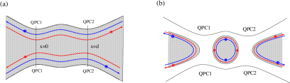
Figure 1: Schematic representation of two quantum point contacts on resonant. (a) weak backscattering limit (b) pinched-off limit.

In addition, recent experimental progresses on transport through multiple constrictions have allowed the study of many interesting physics problems, such as quantum dots, Coulomb blockade, and Kondo problems.Wen (1991); Kane and Fisher (1992a, b); Lee and Toner (1992); Furusaki and Nagaosa (1993a, b); Maciejko et al. (2009); de C. Chamon and Wen (1993) Motivated by this, we are driven to study the case of two constrictions with a geometry as shown in Fig. 1. Using a perturbative renormalization group (RG) transformation,Furusaki and Nagaosa (1993a); Gogolin et al. (1998); Giamarchi (2003) we calculate the conductance when the interacting electrons or quasiparticles are weakly backscattered from the two constrictions. In the opposite limit, when the gate voltages on the two constrictions are increased such that the system is broken down to an island (quantum dot) in between two leads, we use the method of instanton expansion to map the system to its dual field,Rajaraman (1982); Furusaki and Nagaosa (1993a) and calculate the corresponding RG flows in the weak link limit.

Of particular interest is the case where the double constriction is tuned to resonance – in this case, one obtains an emergent Kondo effect on the island between the constrictions. Our analysis therefore is complementary to previous discussions of Kondo impurities in topological insulatorsLaw et al. (2010); Seng and Ng (2011); Chung and Silotri (2012); Eriksson et al. (2012); Posske et al. (2013); Lee and Lee (2013); Chao et al. (2013); Eriksson (2013) which is based on an analysis of the Toulouse point of such models. We also study the case where the constrictions are detuned slightly away from resonance; which in principle can be controlled by a top gate over the island. Over a wide parameter range, we find a metal-insulator transition at some non-zero value of this detuning parameter; we will explain this metal insulator transition and show that it gives rise to an interesting temperature dependence of the Ohmic conductance, $G$.

We further extend the analysis to the more general case of fractional topological insulators (FTIs), in which the filling factor is not an integer number but a fraction with $\nu=1/m$ ($m$ is an odd integer). In this case, the spectrum consists not only of electron like objects, but also quasi-particles with a fractional charge of $\nu e$. Taking quasiparticle tunneling into consideration, we make predictions about the behavior of this exotic phase, should it be found experimentally.

Our paper is organized as follows. In section II, we describe our model, and review the results in Refs. Teo and Kane, 2009; Hou et al., 2009; Ström and Johannesson, 2009. In Sec. III, we study resonant transport properties via two constrictions in QSHIs. In Sec. IV, we discuss our model Hamiltonian and phase diagram for 2D FTIs with a single quantum point contact, and in Sec. IV.2 we generalize to the problem of a double constriction to 2D FTIs. Finally, in Sec. V, we summarize our results and discuss possible future directions.

II Model and review

II.1 Set-up and model Hamiltonian

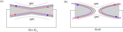
Figure 2: (a) Perfect transmission regime. When the quantum point contact is open, a universal conductance $G_{0}=2\nu\frac{e^{2}}{h}$ is expected to be measured. (b) Perfect reflection regime. When the quantum point contact is pinched off completely, the conductance is zero (in the integer TI case, the quasiparticle is an electron and $\nu=1$).

Before considering the double constriction geometry of Fig. 1, we will set-up the problem and our notation by reviewing the situation with a single constriction present. As shown in Fig. 2, the set-up is that of a two terminal Hall bar connected to a battery. An additional gate, which creates a constriction, is added perpendicular to the Hall bar, allowing for tunneling between the top and the bottom edges at this point. When the constriction is weak as shown in Fig. 2(a), the two terminal conductance is close to the open limit of $G=2e^{2}/h$.Maslov and Stone (1995); Ponomarenko (1995); Safi and Schulz (1995) On the contrary, when the constriction is strong, the geometry is better represented as the pinched-off limit as shown in Fig. 2(b). In this case, the conductance is close to zero.

The helical edge states of the sample can be understood as two copies of integer quantum Hall systems with the two spin states of an electron experiencing opposite effective magnetic fields. We begin with our analysis by defining chiral boson fields $\Phi_{\eta\sigma}$, and the density operator

$$\rho_{\eta\sigma}=\frac{1}{2\pi}\partial_{x}\Phi_{\eta\sigma,}$$ (1)

where $\eta=R,\,L$, and $\sigma=\uparrow,\,\downarrow$. The $R\uparrow$ and $L\downarrow$ states are on the top edge of the sample, while the $R\downarrow$ and $L\uparrow$ states are on the bottom edge. The boson field $\Phi$ satisfies the commutation relation (we use units $\hbar=1$, except for when we write conductance):

$$\left[\Phi_{\eta\sigma}(x),\Phi_{\eta^{\prime}\sigma^{\prime}}(x^{\prime})\right]=\pi i\eta\delta_{\eta\eta^{\prime}}\delta_{\sigma\sigma^{\prime}}\mathtt{sgn}(x-x^{\prime}).$$ (2)

When the short range electron interactions (with interaction strength $\lambda_{2}$ and $\lambda_{4}$ ) are included on the edges, each edge states can be mapped to a spinless Luttinger liquid as follows

$$H=H_{T}+H_{B},$$ (3)

where the Hamiltonian of the top (bottom) edge is

$$H^{T(B)} = \int\mathtt{d}x\left[\pi v_{F}\left(\rho_{R\uparrow(\downarrow)}^{2}+\rho_{L\downarrow(\uparrow)}^{2}\right)\right.$$

$$+ \left.\lambda_{2}\rho_{R\uparrow(\downarrow)}\rho_{L\downarrow(\uparrow)}+\lambda_{4}\left(\rho_{R\uparrow(\downarrow)}^{2}+\rho_{L\downarrow(\uparrow)}^{2}\right)\right].$$

By introducing new boson fields

$$\Phi_{R\uparrow(\downarrow)} = \sqrt{\frac{1}{2}}\left(\theta_{T(B)}-\phi_{T(B)}\right),$$ (5)

$$\Phi_{L\downarrow(\uparrow)} = -\sqrt{\frac{1}{2}}\left(\theta_{T(B)}+\phi_{T(B)}\right),$$ (6)

we diagonalize the total Hamiltonian in Eq. (3) as follows

$$H=\frac{v}{4\pi}\sum_{i=T,B}\int\mathtt{d}x\left[\frac{1}{g}\left(\nabla\theta_{i}\right)^{2}+g\left(\nabla\phi_{i}\right)^{2}\right],$$ (7)

where the boson fields obey a new commutation relation

$$\left[\phi(x),\theta(x^{\prime})\right]=i\pi\mathtt{sgn}(x-x^{\prime}),$$ (8)

and

$$v=v_{F}\sqrt{\left(1+\frac{\lambda_{4}}{\pi v_{F}}\right)^{2}-\left(\frac{\lambda_{2}}{2\pi v_{F}}\right)^{2}},$$ (9)

and

$$g=\sqrt{\frac{1+\lambda_{4}/\pi v_{F}-\lambda_{2}/2\pi v_{F}}{1+\lambda_{4}/\pi v_{F}+\lambda_{2}/2\pi v_{F}}}.$$ (10)

Since constrictions couple top and bottom edges, it is instructive to work with a new basis which is a linear combination of them. This maps the two spinless Luttinger liquids onto a single spinful Luttinger liquid with physical quantities spin $(s)$ and charge $(c)$ density. To account for the distribution of spin between the two edges, the transformation required is:

$$(\theta_{T}+\theta_{B}) = \begin{array}[]{c}\sqrt{2}\theta_{c},\end{array}$$ (11b)

$$(-\theta_{T}+\theta_{B}) = \begin{array}[]{c}\sqrt{2}\phi_{s},\end{array}$$ (11d)

$$(\phi_{T}+\phi_{B}) = \begin{array}[]{c}\sqrt{2}\phi_{c},\end{array}$$ (11f)

$$(-\phi_{T}+\phi) = \begin{array}[]{c}\sqrt{2}\theta_{s}.\end{array}$$ (11h)

Inserting Eqs. (11) into Eq. (7), we obtain a new Hamiltonian with charge (with subscript $c$) and spin (with subscript $s$) sectors as follows:

$$H=\frac{v}{4\pi}\sum_{a=c,s}\int\mathtt{d}x\left[\frac{1}{g_{a}}\left(\nabla\theta_{a}\right)^{2}+g_{a}\left(\nabla\phi_{a}\right)^{2}\right],$$ (12)

where

$$g_{c}=\frac{1}{g_{s}}=g.$$ (13)

The general expression for the original bosonic fields in Eq. (1) in terms of $\theta_{c}$, $\theta_{s}$, $\phi_{c}$ and $\phi_{s}$ is

$$\Phi_{\eta\sigma}=\frac{1}{2}\left[\left(\eta\theta_{c}-\phi_{c}\right)+\sigma\left(\eta\theta_{s}-\phi_{s}\right)\right],$$ (14)

where $\eta=R,\,L=+,-$, and $\sigma=\uparrow,\downarrow=+,-$. In order to complete our bosonized representation of the problem, we must also give the relation between the bosonized fields and the original Fermionic operators:

$$\Psi_{\eta\sigma}=\frac{1}{\sqrt{2\pi\alpha}}e^{i\Phi_{\eta\sigma}}$$ (15)

where $\alpha$ is a short distance cutoff of the field theory. In what follows, we use this notation and the spinful Luttinger Hamiltonian defined in Eq. (12) to carry out the calculations in this report. Unless otherwise stated, we also use the convention that the Fermi velocity $v_{F}=1$.

It is also worth making a comment at this point about our assumption of the conservation of $S_{z}$. In general, two dimensional topological insulators occur in materials with strong spin-orbit coupling, meaning that $S_{z}$ is not conserved. This is crucial when looking at scattering mechanisms on a single edge,Xu and Moore (2006); Wu et al. (2006); Maciejko et al. (2009); Schmidt et al. (2012); Lezmy et al. (2012); Budich et al. (2012) where one must violate conservation of $S_{z}$ in order to get any scattering at all. However, when a constriction is present as we will consider in this work, the dominant scattering mechanism is through the constriction and does not require $S_{z}$ non-conserving terms.Teo and Kane (2009); Eriksson et al. (2012); Eriksson (2013); Lee and Lee (2013) We will therefore not consider this in the current paper.

II.2 Review: single constriction in quantum spin Hall insulator

In this subsection we review the renormalization group flows in the two limits as shown in Fig. 2.Teo and Kane (2009); Ström and Johannesson (2009); Hou et al. (2009) This will form the starting point for extending the results to two constrictions and/or the FTIs. It will also be important to summarize the results here when we later look at off-resonance tunneling through the double constriction in section III.4.

II.2.1 Weak backscattering limit in quantum spin Hall fluids

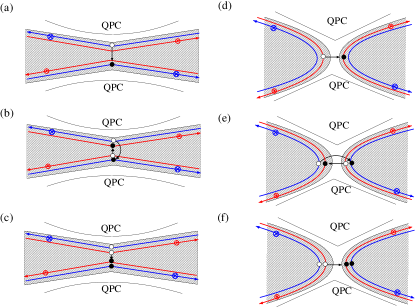
Figure 3: (a-c) Schematic representation of backscattering processes in a near perfectly transmitting phase ($C_{c}C_{s}$). (a) describes the single quasiparticle of charge $\nu e$ tunneling process with perturbation operator $\upsilon_{e}^{q}$ (in the integer TI case, the quasiparticle is an electron and $\nu=1$). When spin is conserved, the particle can either tunnel from $L\uparrow$ to $R\uparrow$ or from $L\downarrow$ to $R\downarrow$. (b) describes a particle pair tunneling process with opposite spins by an operator $\upsilon_{c}^{q}$. (c) describes the transfer of 2 quasiparticles with charge $2\nu e$ from one edge to the other by an operator $\upsilon_{s}^{q}$. (d-f) Schematic representation of tunneling processes in a nearly perfect reflecting phase ($I_{c}I_{s}$). (d) describes single electron tunneling process with perturbation operator $t_{e}$. When spin is conserved, the $\mathit{electron}$ either tunnels from $L\uparrow$ to $R\uparrow$ or from $L\downarrow$ to $R\downarrow$. (e) describes an electron pair tunneling process with opposite spins by a operator $t_{c}$. (f) describes the charge transfer of 2 electrons from one side to the other by an operator $t_{s}$ (in the integer TI case, the quasiparticle is an electron and $\nu=1$).

When the QPC is fully open, a perfect conductance $G=2\frac{e^{2}}{h}$ is expected to be observed.Maslov and Stone (1995); Ponomarenko (1995); Safi and Schulz (1995) However in general, the QPC acts as a local impurity which gives rise to backscattering processes, as shown in Fig. 3. Single backscattering processes as depicted in Fig. 3(a) are always present. However in the presence of interactions, it is also important to consider coherent two-particle backscattering processes illustrated in Figs. 3(b) and 3(c).Teo and Kane (2009) Technically, one may think of these terms as generated by RG transformation.

Taking all these terms into account, the backscattering Hamiltonian is therefore

$$H_{b} = \upsilon_{{}_{e}}\left(\Psi_{R\uparrow}^{\dagger}\Psi_{L\uparrow}+\Psi_{R\downarrow}^{\dagger}\Psi_{L\downarrow}+h.c.\right)$$

$$+2\pi\alpha\upsilon_{{}_{c}}\left(\Psi_{R\uparrow}^{\dagger}\Psi_{R\downarrow}^{\dagger}\Psi_{L\uparrow}\Psi_{L\downarrow}+h.c.\right)$$

$$+2\pi\alpha\upsilon_{{}_{s}}\left(\Psi_{R\uparrow}^{\dagger}\Psi_{L\downarrow}^{\dagger}\Psi_{L\uparrow}\Psi_{R\downarrow}+h.c.\right),$$

$$= \frac{\upsilon_{{}_{e}}}{2\pi\alpha}\cos\theta_{c}\cos\theta_{s}+\frac{\upsilon_{{}_{c}}}{2\pi\alpha}\cos 2\theta_{c}+\frac{\upsilon_{{}_{s}}}{2\pi\alpha}\cos 2\theta_{s}$$

Here $\upsilon_{{}_{e}}$ stands for the $\mathit{single}$ electron backscattering process across the QPC, $\upsilon_{{}_{c}}$ represents a pair backscattering with opposite spins, and $\upsilon_{{}_{s}}$ represents the transfer of 2$e$ charged particles from the top to the bottom edges. The normalization is chosen so as to make all these parameters dimensionless.

The leading order RG flows for each process is as follows:

$$\frac{d\upsilon_{{}_{a}}}{dl}=\left(1-\Delta_{\upsilon a}\right)\upsilon_{{}_{a}},$$ (17)

where $l=\ln\Lambda/T$, and the scaling dimensions are given by:

$$\Delta_{\upsilon e} = \left(g+g^{-1}\right)/2,$$ (18a)

$$\Delta_{\upsilon c} = 2g,$$ (18b)

$$\Delta_{\upsilon s} = 2g^{-1}.$$ (18c)

These equations show that while $\Delta_{\upsilon e}$ is always greater than or equal to one and the single particle backscattering is always irrelevant, the pair backscattering processes may or may not be relevant depending on the value of $g$. For $1/2<g<2$, which includes the case of weak interactions $g\approx 1$, all backscattering processes are irrelevant, and the conducting phase is a stable fixed point. The RG flows for the weak backscattering limit for the full range of interaction $g$ is plotted in the upper part of Fig. 6(a) in Ref. Teo and Kane, 2009.

II.2.2 Weak tunneling limit in quantum spin Hall insulator

When the QPC is completely pinched off, the conductance is expected to be $G=0$ [see geometry in Fig. 3(d) - (f)]. In the vicinity of this point, one allows for weak tunneling between the two halves of the sample. Taking into account both single and two particle processes, as illustrated in Fig. 3(d) - (f), the model Hamiltonian is described as follows:

$$H_{t} = t_{{}_{e}}\left(\Psi_{+\uparrow}^{\dagger}\Psi_{-\uparrow}+\Psi_{+\downarrow}^{\dagger}\Psi_{-\downarrow}+h.c.\right)_{x=0}$$

$$+2\pi\alpha t_{{}_{c}}\left(\Psi_{+\uparrow}^{\dagger}\Psi_{+\downarrow}^{\dagger}\Psi_{-\uparrow}\Psi_{-\downarrow}+h.c.\right)_{x=0}$$

$$+2\pi\alpha t_{{}_{s}}\left(\Psi_{+\uparrow}^{\dagger}\Psi_{-\downarrow}^{\dagger}\Psi_{-\uparrow}\Psi_{+\downarrow}+h.c.\right)_{x=0},$$

$$= \frac{t_{{}_{e}}}{2\pi\alpha}\cos\bar{\phi}_{c}\cos\bar{\phi}_{s}+\frac{t_{{}_{c}}}{2\pi\alpha}\cos 2\bar{\phi}_{c}+\frac{t_{{}_{s}}}{2\pi\alpha}\cos 2\bar{\phi}_{s}.$$

Here $+/-$ represents an infinitesimal displacement from the right and left sides of the QPC located at $x=0$, $\bar{\phi}_{\alpha}=\phi_{\alpha}(+)-\phi_{\alpha}(-)$, $t_{{}_{e}}$ stands for the $\mathit{single}$ $electron$ tunneling process across the QPC, $t_{{}_{c}}$ represents electron pairs tunneling with opposite spins, and $t_{{}_{s}}$ represents the transfer of 2$e$ electron charge from the left to the right sides. As before, the leading order RG flows for each process is:

$$\frac{dt_{{}_{a}}}{dl}=\left(1-\Delta_{ta}\right)t_{{}_{a}},$$ (20)

with scaling dimensions

$$\Delta_{te} = \left(g+g^{-1}\right)/2,$$ (21a)

$$\Delta_{tc} = 2g^{-1},$$ (21b)

$$\Delta_{ts} = 2g.$$ (21c)

For $1/2<g<2$, all tunneling processes are irrelevant, and the insulating phase is a stable fixed point. For more generic $g$, the RG flow is plotted in the lower part of Fig. 6(a) in Ref. Teo and Kane, 2009.

The fact that both the insulating and conducting fixed points are stable for $1/2<g<2$ means that there must be an intermediate unstable fixed point, separating the conducting and insulating phases. This was analyzed in detail in Ref. Teo and Kane, 2009, and the resulting phase diagram is shown in Fig. 6(a) of this work. For later reference, the phase boundary line is also indicated in Fig. 5 of the present paper (see the red dashed curve in the middle of the graph). We follow the notation of Ref. Teo and Kane, 2009 and denote the insulating phase by II and the conducting one by CC. There are also phases which are a charge conductor but spin insulator (CI) and vice versa (IC).

III Transmission through two constrictions and Kondo resonance in integer quantum spin Hall insulators

III.1 Renormalization group flow for the weak backscattering and weak tunneling limits

We now turn to the case of a double constriction as depicted in Fig. 1. Such a double constriction is not only technically feasible in experiments but also contains interesting physics, for example quantum dot physics, Coulomb blockade and Kondo physics. As shown in Fig. 1, this setup is modeled as two tunneling terms between the upper and lower helical edges at locations $x=0$ and $x=d$. After following the previous mapping to the spinful Luttinger liquid, this takes the form of two impurities at these locations, each of which may give rise to backscattering.

Using the standard technique of integrating over degrees of freedom at points other than $x=0,d$, one obtains the local action as follows:Kane and Fisher (1992a); Furusaki and Nagaosa (1993b); Giamarchi (2003)

$$S = S_{0}+\int\mathtt{d}\tau\,V_{eff},$$ (22)

where

$$S_{0} = \frac{1}{\beta}\sum_{\alpha,\omega_{n}}\frac{1}{4\pi g_{\alpha}}\left|\omega_{n}\right|\left|\theta_{\alpha}\left(\omega_{n}\right)\right|^{2},$$ (23)

with $\alpha=+c,-c,+s,-s$, the Matsubara frequencies $\omega_{n}=2\pi nT$, and

$$V_{eff} = V\left(\cos\frac{\theta_{+c}}{\sqrt{2}}\cos\frac{\theta_{-c}}{\sqrt{2}}\cos\frac{\theta_{+s}}{\sqrt{2}}\cos\frac{\theta_{-s}}{\sqrt{2}}\right.$$ (24)

$$\left.+\sin\frac{\theta_{+c}}{\sqrt{2}}\sin\frac{\theta_{-c}}{\sqrt{2}}\sin\frac{\theta_{+s}}{\sqrt{2}}\sin\frac{\theta_{-s}}{\sqrt{2}}\right)$$

$$+\frac{U_{c}}{2}\left(\theta_{-c}-\theta_{-c_{0}}\right)^{2}+\frac{U_{s}}{2}\left(\theta_{-s}-\theta_{-s_{0}}\right)^{2}.$$

In the above expressions, $\theta_{\pm,a}=\left(\theta_{1,a}\pm\theta_{2,a}\right)/\sqrt{2}$, the subscripts $1$ and $2$ denoting the original field operators $\theta_{a}$ at $x=0$ and $x=d$ respectively. The $+$ sign then corresponds to the spin or charge that has been transferred through the junction, and the $-$ sign to the spin or charge between the barriers (we will refer to this region as the quantum dot). The barrier strength is $V$, while $U_{c}$ and $U_{s}$ are phenomenological parameters introduced to describe the interactions (charging energy and exchange energy) of the dot. Finally, $\frac{\sqrt{2}}{\pi}\theta_{-c_{0}}$ and $\frac{\sqrt{2}}{\pi}\theta_{-s_{0}}$ physically correspond to the equilibrium values of charge and spin in the dot and may be controlled via further external gates. We will limit ourselves to the case $\theta_{-s_{0}}=0$, which physically means there is no external magnetic field present.

The weak constriction limit as depicted in Fig. 1(a) corresponds to the case when $V\ll U_{c},U_{s}$ in Eq. (24). One therefore first minimizes the terms involving $U$ and then treats $V$ as a perturbation on top of this. In the particular case where the distance between constrictions $d$ and charging gates are tuned such that

$$\theta_{-c_{0}}=\frac{\pi}{\sqrt{2}}(2n+1)$$ (25)

for any integer $n$, the double constriction is on resonance and the barrier strength $V$ in Eq. (24) does nothing to first order. The present physical picture therefore resembles a single impurity problem, but with the single particle backscattering process removed. The two particle processes however remain: $\upsilon_{c}$ backscattering a pair of electron with opposite spins, and $\upsilon_{s}$ backscattering two electrons from the top to the bottom edges. The scaling dimensions for these two operators are identical to Eqs. (18b) and (18c).

In the strong constriction limit when $V$ is the largest energy scale in the problem, the minimization of the $V$ term in Eq. (24) gives us the conditions that the number of electrons $\frac{\sqrt{2}}{\pi}\theta_{-c}$ and twice the spin $\frac{\sqrt{2}}{\pi}\theta_{-s}$ on the dot are either both even integers, or both odd integers. Further applying the resonance condition in Eq. (25) above means that there are two degenerate spin states of the dot, analogous to a Kondo problem as shown in Fig. 1(b).

Following the same line of reasoning as for the single constriction case, we now identify the possible relevant tunneling processes that may occur in the Kondo limit, and rewrite the problem in this dual description. The details of this are shown in Appendix A, where following the approach of Ref. Teo and Kane, 2009 we obtain the resultant tunneling Hamiltonian

$$H_{t}^{K}=\frac{t_{{}_{e}}}{2\pi\alpha}\cos\bar{\phi}_{+c}\cos\bar{\phi}_{+s}+\frac{\tilde{t}_{{}_{c}}}{2\pi\alpha}\cos\bar{\phi}_{+c}\cos\bar{\phi}_{-s}\\ +\frac{\tilde{t}_{{}_{s}}}{2\pi\alpha}\cos\bar{\phi}_{+s}\cos\bar{\phi}_{-s}.$$ (26)

Here, $\bar{\phi}_{+c}$ and $\bar{\phi}_{+s}$ are fields associated with charge and spin transfer from the left to the right, exactly analogous to the single impurity case in Eq. (II.2.2). The remaining field, $\bar{\phi}_{-s}$ is associated with changes of spin on the dot; and therefore must be treated carefully as there are only two spin states allowed on the dot in the Kondo limit: $\pm 1/2$. More is said about this in Appendix A, where the relationship between Eq. (26) and an instanton expansion of action in Eq. (22) is given.

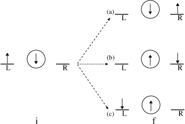
Figure 4: Tunneling processes in the resonant tunneling case, pictorially demonstrating the terms in Eq. (26). Each process is characterized by the charge transferred from left to right, defined as $(\Delta Q_{R}-\Delta Q_{L})/2$, and the spin transferred through the dot defined as $(\Delta S_{R}-\Delta S_{L})/2$. (a) Single electron tunneling process, transferring both spin and charge across the junction; (b) Charge tunneling event, carrying a single charge but no spin across the junction; (c) Spin tunneling event, carrying a single unit of spin but no charge across the junction. Processes (b) and (c) also involve a change of state of the dot.

The physical meaning of the three processes in Eq. (26) is as follows: $t_{e}$ can be thought of a single electron tunneling through the junction without changing the spin of the dot, $\tilde{t}_{{}_{c}}$ refers to a single charge transferred through the junction accompanied by a spin flip both on the dot and the incoming electron, and $\tilde{t}$${}_{{}_{s}}$ involves spin exchange between the dot and one of the leads. These three processes are schematically represented in Fig. 4.

The RG flow equations for this dual picture in Eq. (26) to second order are as follows:

$$\frac{dt_{{}_{e}}}{dl} = \left[1-\frac{1}{2}\left(g+g^{-1}\right)\right]t_{{}_{e}}+AgK_{s}\tilde{t}_{{}_{c}}\tilde{t}_{{}_{s}},$$ (27a)

$$\frac{d\tilde{t}_{{}_{c}}}{dl} = \left[1-\frac{1}{2}\left(K_{s}g+g^{-1}\right)\right]\tilde{t}_{{}_{c}}+Agt_{{}_{e}}\tilde{t}_{{}_{s}},$$ (27b)

$$\frac{d\tilde{t}_{{}_{s}}}{dl} = \left[1-\frac{g}{2}\left(1+K_{s}\right)\right]\tilde{t}_{{}_{s}}+\frac{At_{{}_{e}}\tilde{t}_{{}_{s}}}{g},$$ (27c)

and

$$\frac{dK_{s}}{dl}=-\left(\frac{\tilde{t}_{{}_{c}}^{2}}{g}+g\tilde{t}_{{}_{s}}^{2}\right)K_{s}.$$ (27d)

The parameter $K_{s}$ has the initial condition $K_{s}(l=0)=1$, and appears as a consequence of the special considerations of the $\bar{\phi}_{-s}$ field mentioned above.Kane and Fisher (1992a) The constant $A$ is non-universal; for analysis purposes we take it to be $1$, as the results are not strongly affected by its precise value.

For small $t_{s}$ and $g\neq 1$, the linear terms on the right hand side of Eqs. (27a - 27c) are sufficient to describe the RG flows for the two barriers at resonant case. However for $g\rightarrow 1$, the linear terms on the right hand side vanish, thus those quadratic terms might become important and change the phase boundary. In fact, this will turn out not to be the case, as we show in the next subsection.

III.2 Phase diagram and discussion for resonant double impurity problem

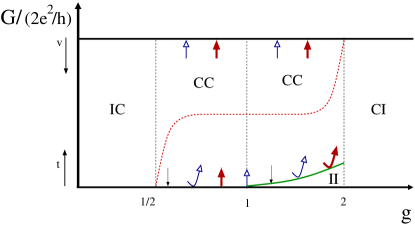
Figure 5: RG flow for a resonant double barrier in an integer QSHI. The result for the weak backscattering limit is shown on the upper part of the figure: blue (with hollow arrow heads) and red arrows are flows for processes transferring two charges and two spins respectively. The result for the weak link limit is shown in the lower part of the figure, where the thin black arrows represent single electron tunneling events, blue arrows (with hollow arrow heads) represent single charge tunneling and thick red arrows represent single spin tunneling events. The green solid line (in the bottom) represents the phase boundary between the conducting and insulating phases for $1<g<2$. For comparison, the red dashed curve (in the middle of the graph) represents the phase boundary for the case of a single constriction.Teo and Kane (2009)

To begin our analysis of the phase diagram for the resonant double constriction, we will ignore the quadratic terms in Eqs. (27a - 27c), or in other words we will start with the case $A=0$. Even with this in mind, the scaling dimension analysis is more complicated than for the single constriction case, as the scaling dimension of the $\tilde{t}_{{}_{c}}$ and $\tilde{t}_{{}_{s}}$ operators depends on the parameter $K_{s}$, which also flows. However, $K_{s}$ always starts at one, and from Eq. (27d) we see that it always flows towards zero (it may however have a limit at some intermediate value). We can therefore look at the scaling dimensions (and therefore the relevance) of the tunneling operators at these two limits of $K_{s}=0,1$. This flow is summarized in Fig. 5 – the curved arrows indicate flow which is initially irrelevant, but some time later in the flow (as $K_{s}$ changes) may become relevant. The figure also shows the stability of the conducting (weak constriction) phase, which is the same as the single barrier case, but with the single electron backscattering removed.

For the weak backscattering limit, the pair backscattering terms are irrelevant under RG for $1/2<g<2$ and we therefore predict that the CC phase is stable in this parameter regime. In the weak link limit however, more interesting things may happen. First, we note that the electron tunneling term $t_{{}_{e}}$ is always irrelevant, and decouples from the equations (when $A=0$), so may be ignored for the present discussion. For $1/2<g<2$, the initial flow of the single charge tunneling term $\tilde{t}_{{}_{c}}$ is towards weak coupling; however as $K_{s}$ decreases this term may become relevant and drive the system towards the CC phase. Now, if $1/2<g<1$, the spin tunneling term $\tilde{t}_{{}_{s}}$ is always relevant and therefore increases to strong coupling. Looking at Eq. (27d), we see that this is sufficient to ensure that $K_{s}$ flows to zero, independent of what happens to the charge tunneling. The charge tunneling term will therefore always become relevant at some energy (temperature) scale, which we will denote $T^{*}$ and discuss below. In this parameter regime, the eventual endpoint of the RG flow is then the stable CC phase.

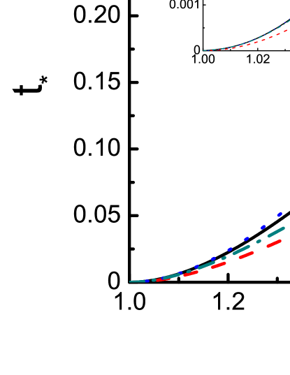
Figure 6: Phase transition boundary between CC and II phases in region $1<g<2$. The figure includes both the upper and lower bounds in Eq. (28) obtained analytically, as well as the results obtained by numerically integrating the RG equations (27) both without ($A=0$) and with ($A=1$) the quadratic terms. The inset zooms into the region around $g\rightarrow 1$ where the critical $t_{*}\rightarrow 0$.

For $1<g<2$, the situation is different, as the initial flow of both $\tilde{t}_{{}_{c}}$ and $\tilde{t}_{{}_{s}}$ is towards zero. The flow of $K_{s}$ depends on the magnitude of $\tilde{t}_{{}_{c}}$ and $\tilde{t}_{{}_{s}}$ – meaning that if these are small (and become smaller under RG), then $K_{s}$ might never decrease below the value needed to turn one of the tunneling terms to be relevant. In other words, there is a phase transition boundary separating an II phase from the CC one. We note that in contrast to the case of a single constriction analyzed in Ref. Teo and Kane, 2009 which found a similar phase boundary at intermediate coupling (also included in Fig. 5 for reference), the present separatrix occurs at weak coupling and therefore can be fully analyzed in the context of the RG equations in Eqs. (27).

Setting $g=1+\varepsilon$ with $\varepsilon\ll 1$, and for convenience assuming the bare tunneling strengths are equal $\tilde{t}_{{}_{c}}=\tilde{t}_{{}_{s}}$ we analytically determine bounds on the critical $t_{*}$ separating flow to the II phase from flow to the CC phase (see Appendix B):

$$\frac{\varepsilon^{2}}{2}<t_{*}<\frac{\varepsilon^{2}}{\sqrt{2}}.$$ (28)

In other words, as $g\rightarrow 1$ from above, the critical tunneling strength approaches zero quadratically. This is compared with the true result obtained by numerical integration of Eq. (27) in Fig. 6.

The above analysis was done ignoring the quadratic terms in Eq. (27), i.e. setting $A=0$. However exactly along the separatrix, the linear term of the equations becomes zero, and therefore it is not a priori obvious that one may ignore the quadratic terms. As it turns out though (see Appendix B), the quadratic nature of $t_{*}$ as shown in Eq. (28) means that along the separatrix, the quadratic terms still remain small, and therefore do not strongly affect the position of the boundary line – in other words, it still goes to zero quadratically as $g\rightarrow 1$. This conclusion is backed up by again numerically solving the RG equations with the quadratic terms $A=1$; this is also plotted in Fig. 6.

We can now understand the full phase diagram of the model of a resonant double constriction as shown in Fig. 5. For $1/2<g<1$, the system always flows to a CC phase, while for $1<g<2$ there is a phase boundary as a function of the strength of the constrictions (controlled by an appropriate gate voltage) between the CC and II phases. Going to stronger interactions and without presenting details, we also find a stable IC phase for $g<1/2$ and a stable CI phase for $g>2$. The calculations are exactly analogous to those done for a single constriction in Ref. Teo and Kane, 2009.

In the language of Kondo physics, the CC phase corresponds to the one-channel Kondo fixed point, while IC is the two-channel Kondo fixed point (see Appendix A). We therefore conclude that the two-channel Kondo fixed point is stable only for $g<1/2$, in strong contrast to recent reportsLaw et al. (2010); Lee and Lee (2013) that the elusive two-channel Kondo fixed point might be accessible for all $g<1$. One possible explanation for this discrepancy is that there is an important difference in the models of those works and that of ours, to do with the size of $J_{1}^{z}$ [see Eq. (51) in appendix A]. We ignore this term [see Eq. (49)], as it does not directly affect transport, and it is marginal so it does not become large under RG flow. On the other hand, the work of Ref. Law et al., 2010 analyzes the stability of Kondo phases by finding exactly solvable (Toulouse) points, which require a large $J_{1}^{z}$. In fact, it has already been advocated by Chung and SilotriChung and Silotri (2012) that there is a quantum phase transition between the one- and two-channel Kondo fixed points in this parameter region. Our work supports this scenario.

III.3 Temperature dependence of conductance for resonant double impurity

Figure 7: Conductance as a function of temperature at $1/2<g<1$ ($g=0.75$ in this plot). In the high temperature regime, there is a power law $G\sim T^{g+1/g-2}$, at intermediate temperature, $G\sim T^{1/g-2}$, and close to zero temperature, $\delta G\sim-T^{4g-2}$ where $\delta G$ is the deviation from perfect conductance. Data points close to the bottom of the graph are not scaled to the data points close to the full conductance.

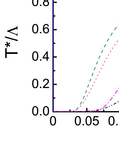
Figure 8: The temperature of minimum conductance $T^{*}$ as a function of bare tunneling strength $t_{0}\equiv\tilde{t}_{c}(l=0)$ for various interaction parameters g.

For most of the phase diagram with $1/2<g<2$ the fixed point of the flow is the conducting one. This means that at $T=0$, one finds perfect conductance through the resonant double impurity. However, if the constrictions are strong, or in other words the conductance at high temperatures is small, then the charge conductance as a function of temperature is non-monotonic. To see this, we recall that the conductance will be proportional to the square of the (renormalized) tunneling strength at the appropriate energy scale

$$G(T)\propto\frac{\tilde{t}_{{}_{c}}^{2}(l)}{1+\tilde{t}_{{}_{c}}^{2}(l)},$$ (29)

where $l=\ln\Lambda/T$. In principle, there is also a term proportional to the electron hopping term $t_{{}_{e}}^{2}$, however as this is always irrelevant it doesn’t play an important role in the following discussion.

Now, while the conducting phase means $\tilde{t}_{{}_{c}}\rightarrow\infty$ as $l\rightarrow\infty$ (i.e. $T\rightarrow 0$), the initial flow of this parameter is in the other direction. By numerically integrating the flow equation (27) one can obtain $G(T)$, as shown in Fig. 7 for a representative value of parameters. In the high temperature regime, the temperature dependence has a form $G\sim T^{g+1/g-2}$, while close to zero temperature, the conductance is determined by the stable CC phase where the correction to the quantized conductance is given by $\delta G\sim-T^{4g-2}$. The most interesting feature of this plot however is the minimum at some flow scale $l^{*}=\ln\Lambda/T^{*}$. This is the scale at which the $\tilde{t}_{{}_{c}}$ operator changes from being irrelevant to being relevant. In physical terms, this temperature give the scale at which the crossover between two channel and one channel Kondo physics (as discussed in the previous subsection) occurs. At temperatures (or energy scales) higher than $T^{*}$, the physics appears to be that of the two channel Kondo model — however at lower temperatures, the one channel Kondo physics takes over.

Numerically, $T^{*}$ can be determined as a function of the bare tunneling $t_{0}\equiv\tilde{t}_{{}_{c}}$ and Luttinger constant $g$, as shown in Fig. 8. We can also obtain analytic expressions for $T^{*}$ in various limits (see Appendix C). If $g=1+\varepsilon$, we find in the limit $\varepsilon/t_{0}\ll 1$:

$$T^{*}\sim\Lambda\left(1-\frac{\varepsilon^{2}}{2t_{0}^{2}}\right).$$ (30)

For any real material, the cutoff $\Lambda$ may be taken to be the bulk energy gap. For HgCdTe this is about 40 meV, meaning that the temperature of minimum conductance is of the order of one hundred Kelvin, so long as the bare (high temperature) conductance is not too small.

In the opposite limit of $\varepsilon/t_{0}\gg 1$, and $g<1$, we find

$$T^{*}\sim\Lambda t_{0}^{\frac{1}{1-g}},$$ (31)

with the minimum conductance $G_{\mathrm{min}}=G(T^{*})$ given by

$$G_{\mathrm{min}}\sim t_{0}^{\frac{g+1}{g}}.$$ (32)

Such a limit does not exist for $g>1$, as there is no $T^{*}$ within the II phase. However, we can say that close to the phase transition on the CC side, $T^{*}$ is very small, going to zero exactly at the phase boundary.

At temperature below $T^{*}$, when the system now behaves like the one channel Kondo model, there is another important temperature – the Kondo temperature $T_{K}$. This is defined as the energy scale when $\tilde{t}_{{}_{c}}(T_{K})=1$; or in other words, the strong coupling regime is reached. As we will show in the next subsection, this energy scale is crucial when describing the physics of the double constriction tuned slightly off resonance. We will therefore now briefly discuss the Kondo temperature in our model, for a derivation of these results see Appendix C. When $g$ is close to or greater than $1$, there is not a great separation of energy scales between $T^{*}$ and $T_{K}$. Hence to within prefactors of the order of unity, these energy scales are the same. However, under the same conditions of validity as Eq. (31), we find that

$$T_{K}\sim T^{*}\,t_{0}^{\frac{1+g}{2g-1}}=\Lambda t_{0}^{\frac{g(2-g)}{(2g-1)(1-g)}},$$ (33)

and therefore there is a parametrically large region between the minimum of conductance, $T^{*}$, and the strong coupling regime $T_{K}$, where the physics of the CC point takes over. In this intermediate temperature range, there is a third power law (beyond the high and low temperature limits mentioned previously), $G\sim T^{1/g-2}$. In a system with sufficiently strong constrictions, all three of these power laws should be seen clearly, giving an experimental signature for the presence of the helical LL edge states, as well as a consistency check for the experimental determination of $g$. The main downside of this scheme is that the stronger the constriction (and therefore the wider the power law regions), the lower the temperature scales relevant for the crossovers.

III.4 Double constriction tuned slightly off resonance

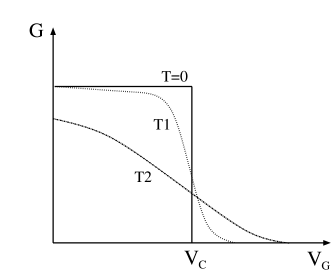
Figure 9: Schematic plot of the metal insulator transition: conductance as a function of detuning from resonance $V_{G}$. At zero temperature, there exhibits a sharp metal insulator transition at $V_{C}$, but at finite temperatures this sharp transition becomes a crossover.

We now add a twist to the problem of a double constrictions by considering that the resonant condition in Eq. (25) is almost, but not quite, satisfied. This may be tuned in an experiment by yet another gate capacitively coupled to the dot, and therefore changing the equilibrium charge in the dot away from the odd integer required for resonance. We introduce a physical parameter $V_{G}$, which can be controlled by a top gate over the dot, to quantify the distance from resonance, in other words $V_{G}$ is the energy difference between the two lowest energy states within the dot.

If $V_{G}$ is very large (i.e. the system is far from resonance), then there are no internal dynamical processes within the dot, and the double constriction looks identical to a single constriction with some effective tunneling across it. This motivates the use of a two-cutoff RG procedure. At energy scales larger than $V_{G}$, the system doesn’t sense the perturbation and it looks exactly like the case of resonance. Therefore the RG equations in Eq. (27) for the resonant case are used. However when the energy scale is lower than $V_{G}$ , the system behaves like a single constriction, so the RG equations are switched to those for a single constriction [see Eqs. (17) and (21)].

For $1/2<g<2$, we show in Fig. 5, the phase boundary lines between insulating and conducting phases for both the resonant double constriction case (as discussed above), and the single constriction case (after Ref. Teo and Kane, 2009). By far the most interesting region of the phase diagram is the large region of phase space between the red dashed and green solid lines where the resonant constriction conducts, while the single constriction is an insulator. In other words, if the detuning from resonance is introduced then the system is a conductor at $V_{G}=0$ but an insulator when $V_{G}$ is large. This implies that there must be a critical detuning $V_{C}$ where the system undergoes a metal-insulator transition. Of course, this is a transition only at zero temperature $T=0$, at non-zero temperatures it becomes a crossover as shown schematically in Fig. 9.

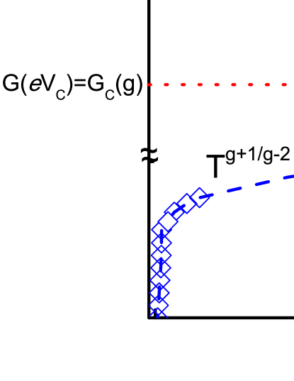
Figure 10: Conductance vs temperature at small detuning from resonance, $V_{G}$. For $T\gg V_{G}$, the system is described as if it were resonant, but for $T\ll V_{G}$ the system effectively looks like a single constriction. When $V_{G}$ is smaller than some critical $V_{C}$ the system is conducting otherwise the system flow is insulating. Numerical data obtained by integrating the RG equations is represented by blue squares, red diamonds, and green circles (Data points close to the bottom of the graph are not scaled to the data points close to perfect conductance).

The value of $V_{C}$ may be estimated via the two-cutoff RG procedure outlined above. Basically, the bare parameters flow initially under the resonant RG equations in Eq. (27) from an energy scale (or temperature) $\Lambda$ down to $V_{G}$. At this energy scale, one switches to the physics of the single constriction – so in order for the system to remain metallic, the renormalized conductance at this energy scale must be bigger than the critical conductance $G_{C}(g)$ for the metal-insulator transition in the single constriction case, as found by Teo and Kane in Ref. Teo and Kane, 2009. Hence the critical $V_{C}$ is given by the matching condition

$$G(T=eV_{C})=G_{C}(g).$$ (34)

When $V_{G}<V_{C}$, the system flows to conducting fixed point, while for $V_{G}>V_{C}$, the system flows to insulating fixed point.

As can be seen from Fig. 5, the critical conductance for the single constriction $G_{C}(g)\sim 1/2$, so long as $g$ is not too close to either $1/2$ or $2$; in other words, the phase boundary lies at intermediate coupling. Now, the energy scale at which this happens is exactly the Kondo temperature, as we defined it in the previous section. Hence, over a wide range of values of interaction $g$ and up to numerical prefactors of the order of unity, $V_{C}\sim T_{K}/e$. Hence by detuning the constrictions from the resonance transition, one makes a direct probe of the Kondo temperature of the system.

The behavior of conductance as a function of temperature is shown for both these cases in Fig. 10. It is worth commenting that for $V_{G}>V_{C}$, the conductance as a function of temperature shows a local maximum at $T\sim eV_{G}$. This is on top of the local minimum that occurs at $T=T^{*}$ due to Kondo physics, giving a rather interesting profile to the $G-T$ characteristics of the system, which should be observable experimentally.

Figure 11: Conductance on the critical line $V_{G}=V_{C}$. When the system is tuned to this condition, the single-constriction metal-insulator phase boundary acts as an attractive fixed fixed. Here we plot three various initial tunneling strength along this critical line. The ultimate conductance at $T=0$ is given by $G_{C}(g)$. In this plot, $g=0.75$.

Finally, we mention the interesting possibility of tuning the system exactly to the critical line where $V_{G}=V_{C}$. With this condition satisfied, the metal-insulator boundary found in Ref. Teo and Kane, 2009 acts as an attractive fixed point; the ultimate $T=0$ conductance is given by this value. Some typical plots of conductance as a function of temperature on this critical line are given in Fig. 11. We leave a full analysis of the scaling behavior expected here for future work.

IV 2d fractional topological insulators

We now turn to the case of adding constrictions to 2D FTIs with a filling factor $\nu=1/m$ ($m$ is an odd integer). We first discuss the appropriate model of such a state of matter, before adding a single constriction and then a resonant double constriction as discussed above for the integer case. The analysis will be very similar to the integer case: first bosonize the model in the absence of constrictions, then add constrictions and use an RG analysis to study the stability of the weak and strong coupling fixed points, which allows us to draw the phase diagram. We will therefore concentrate on what changes when one moves from the integer to the fractional cases; for details of the calculations, see the previous sections.

As proposed by Levin and Stern,Levin and Stern (2012) a toy model of a 2D FTI is made from two copies of a fractional quantum Hall state with opposite spin species, and a short range interaction between them. Within this model, the filling factor $\nu$ modifies the Hamiltonian in Eq. (II.1) as follows:Wen (1990, 1992)

$$H^{T(B)} = \int\mathtt{d}x\left[\frac{\pi v_{F}}{\nu}\left(\rho_{R\uparrow(\downarrow)}^{2}+\rho_{L\downarrow(\uparrow)}^{2}\right)\right.$$

$$+ \left.\lambda_{2}\rho_{R\uparrow(\downarrow)}\rho_{L\downarrow(\uparrow)}+\lambda_{4}\left(\rho_{R\uparrow(\downarrow)}^{2}+\rho_{L\downarrow(\uparrow)}^{2}\right)\right],$$

where the density $\rho$ is now given by

$$\rho=\frac{\sqrt{\nu}}{2\pi}\partial_{x}\Phi_{\eta\sigma},$$ (36)

in terms of boson fields $\Phi_{\eta\sigma}$ satisfying the commutation relation in Eq. (2). The electron creation operator is modified to

$$\Psi_{e,\eta\sigma}^{\dagger}=e^{-i\frac{\Phi_{\eta\sigma}}{\sqrt{\nu}}},$$ (37)

and the quasiparticle creation operator with fractional charge $\nu e$ is

$$\Psi_{q,\eta\sigma}^{\dagger}=e^{i\sqrt{\nu}\Phi_{\eta\sigma}}.$$ (38)

The chiral boson fields can further be expressed as before by Eq. (14).

Going through these transformations, the Hamiltonian in Eq. (IV) once more splits into a spin and charge part as written in Eq. (12) but with a modification of the parameters:

$$g=\sqrt{\frac{1+\lambda_{4}/\pi\nu v_{F}-\lambda_{2}/2\pi\nu v_{F}}{1+\lambda_{4}/\pi\nu v_{F}+\lambda_{2}/2\pi\nu v_{F}}},$$ (39)

and

$$v=v_{F}\sqrt{\left(1+\frac{\lambda_{4}}{\pi\nu v_{F}}\right)^{2}-\left(\frac{\lambda_{2}}{2\pi\nu v_{F}}\right)^{2}}.$$ (40)

Note that if we put $\nu=1$, we recover the expressions in Eqs. (9) and (10) of the integer case.

IV.1 Single constriction

We now add a single constriction (with geometry as shown in Fig. 2) to the FTI. Before plugging the modified operators in Eqs. (37) and (38) into the previous expressions, there is one final point to mention, which is under which circumstances may fractionally charged quasi-particles be backscattered (or tunnel), and in which cases are only electrons allowed. This has recently been discussed by Beri and Cooper in Ref. Beri and Cooper, 2012 for magnetic impurities in a single edge, where the two species (spin up and spin down) of electrons or quasi-particles must scatter into each other. The present case is much simpler, as the scattering between the top and lower edges preserves the species index of the particles being scattered. Consequently, we can use the conventional wisdom from fractional quantum Hall systemsDas Sarma and Pinczuk (1997) and observe that the scattering from the upper to lower edges in the weak backscattering limit may be quasiparticles, while only electrons may tunnel between the left and right of a system that has been pinched off.

With this information, we are now ready to modify the calculations presented above for the fractional case. In the weak backscattering limit, quasiparticles are scattered between the upper and lower edges. Substituting the quasi-particle operator in Eq. (38) for $\Psi$ in Eq. (II.2.1), we obtain the quasiparticle backscattering Hamiltonian

$$H_{b}^{F}=\frac{\upsilon_{{}_{e}}^{q}}{2\pi\alpha}\cos\sqrt{\nu}\theta_{c}\cos\sqrt{\nu}\theta_{s}+\frac{\upsilon_{{}_{c}}^{q}}{2\pi\alpha}\cos 2\sqrt{\nu}\theta_{c}\\ +\frac{\upsilon_{{}_{s}}^{q}}{2\pi\alpha}\cos 2\sqrt{\nu}\theta_{s},$$ (41)

where $\upsilon_{{}_{e}}^{q}$ stands for the single quasiparticle backscattering process across the QPC, $\upsilon_{{}_{c}}^{q}$ represents a quasiparticle pair backscattering with opposite spins, and $\upsilon_{{}_{s}}^{q}$ represents the transfer of 2$\nu e$ charged particles from the top to the bottom edges. The leading order renormalization group flows for each process is then

$$\frac{d\upsilon_{{}_{a}}^{q}}{dl}=\left(1-\Delta_{\upsilon a}^{(q)}\right)\upsilon_{{}_{a}}^{q},$$ (42)

with scaling dimensions

$$\Delta_{\upsilon e}^{(q)} = \frac{\nu}{2}\left(g+g^{-1}\right),$$ (43a)

$$\Delta_{\upsilon c}^{(q)} = 2\nu g,$$ (43b)

$$\Delta_{\upsilon s}^{(q)} = 2\nu g^{-1}.$$ (43c)

On the contrary, in the weak link limit, quasiparticle tunneling between the two fractional fluids is forbidden, so the tunneling Hamiltonian involves only electron operators

$$H_{t}^{F}=\frac{t_{{}_{e}}}{2\pi\alpha}\cos\frac{\bar{\phi}_{c}}{\sqrt{\nu}}\cos\frac{\bar{\phi}_{s}}{\sqrt{\nu}}+\frac{t_{{}_{c}}}{2\pi\alpha}\cos\frac{2\bar{\phi}_{c}}{\sqrt{\nu}}\\ +\frac{t_{{}_{s}}}{2\pi\alpha}\cos\frac{2\bar{\phi}_{s}}{\sqrt{\nu}}.$$ (44)

Here the labeling is the same as the integer case. The scaling dimensions of these operators are:

$$\Delta_{te}^{(q)} = \frac{1}{2}\nu^{-1}\left(g+g^{-1}\right),$$ (45a)

$$\Delta_{tc}^{(q)} = 2\nu^{-1}g^{-1},$$ (45b)

$$\Delta_{ts}^{(q)} = 2\nu^{-1}g.$$ (45c)

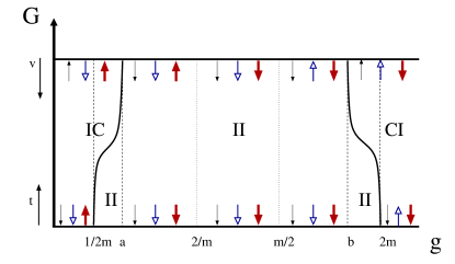
Figure 12: Phase diagram for a point contact in a FTI as a function of Luttinger constant $g$. The points $a=m-\sqrt{m^{2}-1}$ and $b=m+\sqrt{m^{2}-1}$. The result for the weak backscattering limit is shown on the upper part of the figure, and the result for the weak link limit is shown in the lower part of the figure. Thin black arrows represent single electron processes, blue arrows (with hollow arrow heads) represent charge tunneling (or backscattering) and thick red arrows represent spin tunneling (or backscattering) events. The black solid curves indicate schematically the phase boundary between the IC and II phases for $1/2m<g<a$, and between the CI and II phases for $b<g<2m$. A stable insulating phase is found for all $a<g<b.$

The phase diagram for a 2D FTI is obtained by analyzing the stability of these two limits, and is plotted in Fig. 12. As shown in the upper panel of the figure (weak backscattering limit), the single particle backscattering operator with strength $\upsilon_{e}^{q}$ becomes relevant when $m-\sqrt{m^{2}-1}<g<m+\sqrt{m^{2}-1}$, which doesn’t happen in the case of integer QSHIs. The operator coupled to $\upsilon_{c}^{q}$ is relevant when $g<m/2$ , and that coupled to $\upsilon_{s}^{q}$ becomes relevant when $g>2/m$. In the other limit on the bottom panel of the plot, the parameter $t_{e}$ is irrelevant for any $g$, while $t_{c}$ becomes relevant when $g>2m$ and $t_{s}$ is relevant for $g<1/2m$. We find that in the most likely physical regime of $g$ not too far from one, there exists a stable insulating phase. It coincides with the prediction in the fractional quantum Hall effect in which a even a weak impurity will drive the fractional quantum Hall fluid to an insulating phase.Das Sarma and Pinczuk (1997)

IV.2 Resonant double constriction

Finally, we consider a resonant double constriction for a FTI, with a geometry as shown in Fig. 1. As before, in the weak backscattering limit one considers quasiparticle processes, and the effective action in Eq. (22) is modified by $\theta\rightarrow\sqrt{\nu}\theta$. Again, the resonant condition means that the single particle backscattering process is absent, and the scaling dimensions for the two particle processes are as for the single constriction case

$$\Delta_{\upsilon c}^{(q)} = 2\nu g,$$ (46a)

$$\Delta_{\upsilon s}^{(q)} = 2\nu g^{-1}.$$ (46b)

For the weak link limit, only electron processes are allowed, which means $\bar{\phi}$ is modified by $\bar{\phi}/\sqrt{\nu}$ in Eq. (26). The scaling dimensions for the three tunneling processes are as follows:

$$\Delta_{te}^{(q)} = \frac{1}{2\nu}\left(g+g^{-1}\right),$$ (47a)

$$\Delta_{tc}^{(q)} = \frac{1}{2\nu}\left(K_{s}g+g^{-1}\right),$$ (47b)

$$\Delta_{ts}^{(q)} = \frac{g}{2\nu}\left(1+K_{s}\right).$$ (47c)

The way that the full RG equations (including the flow of $K_{s}$) given for the integer case in Eq. (27) is modified is clear from the above expressions. We also note that these electronic tunneling processes are still correctly given by the instantons of the potential in Eq. (26) with the quasiparticle modification above; meaning that our picture of quasiparticles and electrons is a consistent one.

The RG flow is summarized in Fig. 13, where we predict an insulating phase occurs when $2/m<g<m/2$. At $g<2/m$ there is a transition to the IC phase, while a transition to the CI phase occurs at $g>m/2$ – although neither of these transition lines is vertical. In the CI phase, we predict a non-monotonic temperature dependence of charge conductance, while the IC phase exhibits non-monotonic temperature dependence of spin conductance, so long as $g>1/m$. We note that unlike the integer case, all this interesting behavior happens at strong interaction strengths, of $g$ not close to one.

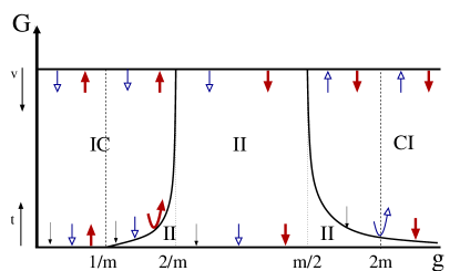
Figure 13: RG flow for a double barrier in a FQSHI. The result for the weak backscattering limit is shown on the upper part of the figure: blue (with hollow arrow heads) and red arrows are flows for processes involving two charges and two spins respectively. The result for the weak link limit is shown in the lower part of the figure, where the thin black arrows represent single electron tunneling events, blue arrows (with hollow arrow heads) represent single charge tunneling and thick red arrows represent single spin tunneling events. The shapes of the thick black phase boundary lines between the IC, II and CI phases are schematic. In the regions with curved arrows, we predict non-monotonic temperature dependence of conductance: charge conductance in the CI phase, and spin conductance in the IC phase (with g>1/m).

V Summary

In summary, we have considered a quantum spin Hall insulator with a double constriction as shown in Fig. 1. The transport properties of the setup are controlled by three parameters: the interaction strength within the material parametrized as the Luttinger liquid constant $g$, strength of the constrictions $\upsilon$, and how close the system is to resonance $V_{G}$. The former is an intrinsic property of the material (although may be partially controlled via screening through metal gates in close proximity), however the latter two may be easily controlled experimentally through appropriate side and top gates on the sample.

We find that if $1/2<g<1$ the system is always conducting at resonance, though with conductance non-monotonic as a function of temperature due to Kondo physics. Unlike some recent reports however, we do not find the two-channel Kondo fixed point stable in this region – this may be due to an interaction between the dot and the leads which we consider to be small, while previous studies have taken it to be large. We believe the most likely scenario is a quantum phase transition as a function of this interaction, however more work needs to be done in this direction.

Our conducting phase may be driven to an insulating phase by tuning $V_{G}$, with a metal-insulator transition at some critical $V_{G}=V_{C}$. On the insulating side of the transition, the conductance as a function of temperature has both a maximum and a minimum (see Fig. 10); we believe this to be a fascinating experimental signature of the physics discussed in this work.

Finally, we studied the same geometry for the as yet hypothetical fractional topological insulators with filling fraction $\nu=1/m$, $m$ being an odd integer. In this case, we find that all of the exciting physics of the integer case has moved to much higher interaction strengths; for $2/m<g<m/2$ we predict a stable insulating phase. It appears to be a curious characteristic of the fractional TI edge states that while single edges show a remarkable resilience to single edge perturbations,Beri and Cooper (2012) they are completely unstable to a coupling between two edges.

Appendix A Derivation of the Kondo Hamiltonian

As in the case of a single constriction, if the constrictions are very large then it is more convenient to begin from the completely pinched off limit and add in the weak tunneling between the leads and the dot perturbative. The tunneling Hamiltonian takes the form

$$H_{tun}=T_{L}\sum_{\sigma}\Psi_{1\sigma}^{\dagger}\Psi_{d\sigma}+T_{R}\sum_{\sigma}\Psi_{2\sigma}^{\dagger}\Psi_{d\sigma}+h.c.,$$ (48)

where $\Psi_{1\sigma}$, $\Psi_{2\sigma}$, and $\Psi_{d\sigma}$ annihilate an electron with spin $\sigma$ on the left, right leads and the dot respectively, and we have allowed different tunneling amplitudes $T_{L}$ and $T_{R}$ through the left and right constriction respectively. However this is not the full story, as the resonance condition in Eq. (25) ensures that the dot has a fixed odd number of electrons sitting on it, with some charging energy $U$ to add (or remove) an electron from it. The odd number means that there is still an internal degree of freedom on the dot – the spin – which has two degenerate states [see Eqs. (24) and (25)].

Restricting ourselves to low energies, one therefore looks at the second order processes in which the final state of the dot remains within the low energy manifold. Applying second order perturbation theory generates the following four operators:

$$H_{e}^{K} = -\frac{T_{L}T_{R}^{*}}{U}\sum_{\sigma}\Psi_{1\sigma}^{\dagger}\Psi_{2\sigma}\left(1-\Psi_{d\sigma}^{\dagger}\Psi_{d\sigma}\right)$$

$$\quad\quad-\frac{T_{L}^{*}T_{R}}{U}\sum_{\sigma}\Psi_{2\sigma}^{\dagger}\Psi_{1\sigma}\left(1-\Psi_{d\sigma}^{\dagger}\Psi_{d\sigma}\right),$$

$$H_{c}^{K} = \frac{T_{L}T_{R}^{*}}{U}\sum_{\sigma}\Psi_{1\sigma}^{\dagger}\Psi_{2-\sigma}\Psi_{d-\sigma}^{\dagger}\Psi_{d\sigma}$$

$$\quad\quad+\frac{T_{L}^{*}T_{R}}{U}\sum_{\sigma}\Psi_{2\sigma}^{\dagger}\Psi_{1-\sigma}\Psi_{d-\sigma}^{\dagger}\Psi_{d\sigma},$$

$$H_{s}^{K} = \frac{\left|T_{L}\right|^{2}}{U}\sum_{\sigma}\Psi_{1\sigma}^{\dagger}\Psi_{1-\sigma}\Psi_{d-\sigma}^{\dagger}\Psi_{d\sigma}$$

$$\quad\quad+\frac{\left|T_{R}\right|^{2}}{U}\sum_{\sigma}\Psi_{2\sigma}^{\dagger}\Psi_{2-\sigma}\Psi_{d-\sigma}^{\dagger}\Psi_{d\sigma}.$$

$$H_{dd} = \frac{\left|T_{L}\right|^{2}}{U}\sum_{\sigma}\Psi_{1\sigma}^{\dagger}\Psi_{1\sigma}\Psi_{d\sigma}^{\dagger}\Psi_{d\sigma}$$

$$\quad\quad+\frac{\left|T_{R}\right|^{2}}{U}\sum_{\sigma}\Psi_{2\sigma}^{\dagger}\Psi_{2\sigma}\Psi_{d\sigma}^{\dagger}\Psi_{d\sigma}.$$

The physical meaning of each of the first three terms is explained in the main text and schematically represented in Fig. 4. For the symmetrical case when both constrictions are identical, $T_{L}=T_{R}=T_{0}$, and the bare $t_{\alpha}$ all have transmission strengths proportional to $\left|T_{0}\right|^{2}$. The fourth term, Eq. (49), takes the form of an $S^{z}S^{z}$ interaction. This term does not transfer any spin or charge across the dot, and furthermore is marginal under RG which we use as justification for neglecting it. However, if for whatever reason the bare value of this fourth term is large, its presence may have an important influence on the RG flow of the other terms (see discussion in main text). A careful study of the effect of this term is however beyond the scope of the present work.

Following the same procedure as for the single constriction case, we then bosonize the first three tunneling terms above, arriving at the answer

$$H_{t}^{K}=\frac{t_{{}_{e}}}{2\pi\alpha}\cos\bar{\phi}_{+c}\cos\bar{\phi}_{+s}+\frac{\tilde{t}_{{}_{c}}}{2\pi\alpha}\cos\bar{\phi}_{+c}\cos\bar{\phi}_{-s}\\ +\frac{\tilde{t}_{{}_{s}}}{2\pi\alpha}\cos\bar{\phi}_{+s}\cos\bar{\phi}_{-s}.$$ (50)

which is quoted in Eq. (26) in the main text. Care must be taken however to understand the difference between the fields $\bar{\phi}_{+c},\bar{\phi}_{+s}$ and the field $\bar{\phi}_{-s}$. The first two are associated with tunneling of charge or spin from the left to the right leads, and are no different from the equivalent operators found in the single constriction case. The remaining field however $\bar{\phi}_{-s}$ is associated with the state of the dot. In fact, bosonizing the dot which is not a bulk system (in contrast to the semi-infinite leads) is somewhat of a cheat; however continuing this line of reasoning we are led to the following important point. While a local operator in a one-dimensional wire can not renormalize the Luttinger liquid constant of the wire, this is not true of the operator $\cos\bar{\phi}_{-s}$ on the dot. Consequently, one should define an effective Luttinger liquid parameter of the dot, $K_{s}g$ (where the bare value of $K_{s}=1$), which may change during the renormalization procedure. This is one way to understand the parameter $K_{s}$ appearing in the RG equations (27) in the main text.

While the above argument for the introduction of $K_{s}$ turns out to be mathematically correct, it clearly lacks rigor. This may be rectified by looking at the problem from a different angle. By going back to the original action in terms of the constrictions Eq. (22) and performing saddle point approximation on the second term,Rajaraman (1982); Schmid (1983); Furusaki and Nagaosa (1993a); Giamarchi (2003) we can write down trajectories for six instantons between successive minimal of the cosine potentials (our choice of resonance condition means that processes involving $\theta_{-c}$ that change the charge on the dot are less important than other terms). Furthermore, the operator $\cos\bar{\phi}_{+c}$ in Eq. (50) is exactly the operatorSaleur (1999) that creates a half-instanton in the original $\cos\theta_{+c}/\sqrt{2}$ potential, and similarly for the other two fields. In this sense, the perturbation (Coulomb gas) expansion of the tunneling Hamiltonian Eq. (50) is identical to the instanton expansion of Eq. (22), so one may regard $t_{{}_{e}}$, $\tilde{t}_{{}_{c}}$ and $\tilde{t}_{{}_{s}}$ as the fugacities of instantons in the original problem. Again we see why there must be special treatment of the $\theta_{-s}$ (or in the dual problem $\bar{\phi}_{-s}$) field: there are only two allowed spin states of the dot, so the time ordering in this field must alternate between instantons and anti-instantons. Treating this carefullyKane and Fisher (1992a) requires the introduction of a new parameter $K_{s}$ into the RG equations in Eqs. (27).

Finally, we show the relation between our notation and that of the two-channel Kondo model. As the dot has only two states, we can replace all operators on the dot (in the low energy limit) by a single spin-half operator $\vec{S}$. The standard notation for the Kondo Hamiltonian is then

$$H^{K}=\sum_{i=1,2}J_{1}\vec{S}\cdot\left(\Psi_{i\sigma}\vec{\sigma}_{\sigma\sigma^{\prime}}\Psi_{i\sigma^{\prime}}\right)+\sum_{i\neq j}J_{2}\vec{S}\cdot\left(\Psi_{i\sigma}\vec{\sigma}_{\sigma\sigma^{\prime}}\Psi_{j\sigma^{\prime}}\right)$$ (51)

Comparing with our terms, we therefore see that $J_{1}^{xy}=\tilde{t}_{{}_{s}}$, $J_{2}^{z}=t_{{}_{e}}$ and $J_{2}^{xy}=\tilde{t}_{{}_{c}}$. The term we neglect is $J_{1}^{z}$.

Looking at Eq. (51), we see that the $J_{1}$ terms are the traditional Kondo spin-exchange couplings to the two leads, while the $J_{2}$ terms are those that allow for charge transport. The two-channel Kondo fixed point is therefore the one where $J_{2}=0$, i.e. only the Kondo couplings remain, and furthermore flow to strong coupling. This is exactly the phase we call IC – note that while the II phase also has $J_{2}\rightarrow 0$ under RG, in this case $J_{1}$ also flows to weak coupling which is the decoupled dot fixed point and not a Kondo-like one. On the other hand, if both $J_{1}$ and $J_{2}$ flow to strong coupling, this is the single channel Kondo fixed point.Glazman and Raikh (1988); Ng and Lee (1988)

Appendix B Analytical analysis of the separatix line between the CC and II phases at $1<g<2$

In this appendix, we derive the limits of the phase boundary in Eq. (28) in the main text by giving an approximate analytic solution to the flow equations in Eq. (27).

Without the quadratic terms $A=0$, the flow equation for $t$${}_{{}_{e}}$ (27a) decouples from the rest and always flows to weak coupling. However, the flow of $\tilde{t}_{{}_{c}}$ and $\tilde{t}_{{}_{s}}$ are less trivial since they both depend on $K$. To make progress, we rearrange Eqs. (27b - 27d) as follows,

$$\frac{d\tilde{t}_{{}_{c}}}{dl}-a\tilde{t}_{{}_{c}} = -\frac{K_{s}g}{2}\tilde{t}_{{}_{c}},$$ (52)

$$\frac{d\tilde{t}_{{}_{s}}}{dl}-b\tilde{t}_{{}_{s}} = -\frac{K_{s}g}{2}\tilde{t}_{{}_{s}},$$ (53)

where $a=1-\frac{1}{2g}$, and $b=1-\frac{g}{2}$.

Introducing new variables

$$X=\tilde{t}_{{}_{c}}e^{-al},\quad\quad Y=\tilde{t}_{{}_{s}}e^{-bl},$$

we find

$$\frac{dX}{dl} = -\frac{K_{s}g}{2}X,$$ (54a)

$$\frac{dY}{dl} = -\frac{K_{s}g}{2}Y.$$ (54b)

Dividing Eq. (54a) by Eq. (54b) gives $dX/dY=X/Y$ which has the solution $X=cY$ for some constant $c$. Hence transforming back to our original variables gives

$$\tilde{t}_{{}_{s}}(l)=\tilde{t}_{{}_{c}}(l)e^{(b-a)l},$$ (55)

and our problem now reduces to solving two coupled differential equations for $\tilde{t}_{{}_{c}}$ and $K_{s}$. The equation for the former is given in Eq. (52) while the latter now satisfies

$$\frac{dK_{s}}{dl}=-\left(\frac{1}{g}+g\alpha(l)\right)\tilde{t}_{{}_{c}}^{2}K_{s},$$ (56)

where $\alpha(l)=\frac{\tilde{t}_{{}_{s}}^{2}(0)}{\tilde{t}_{{}_{c}}^{2}(0)}e^{2(b-a)l}$ which falls between $0$ and $\alpha_{\mathrm{max}}$ for $l>0$ as long as $g>1$. In the case that the bare tunneling terms are identical, $\alpha_{\mathrm{max}}=1$.

We are interested in the fixed point of the flow in Eqs. (52) and (56) in the limit $l\rightarrow\infty$. There are two possibilities: either $\tilde{t}_{{}_{c}}\rightarrow\infty$ and $K_{s}\rightarrow 0$ which is the conducting phase, or $\tilde{t}_{{}_{c}}\rightarrow 0$ with $K_{s}\rightarrow K_{*}$. It is not difficult to conclude that in the region of interest, $1<g<2$, one must have $K_{*}>0$. We now understand the shape of the flow of the equations – as $l$ grows, $K_{s}$ decreases; if it decreases past a certain point then the eventual fixed point is ultimately the conducting one. This invites an easy approximation to allow us to approximately locate the phase boundary: if we neglect the flow of $\alpha$, i.e. let $\alpha(l)=\alpha_{\mathrm{max}}$, then the negative flow of $K$ will be faster than the true flow, and we will underestimate the critical bare $\tilde{t}_{{}_{c}}$ needed for the system to reach the strong coupling fixed point. On the other hand, simply putting $\alpha=0$ will do the opposite, and overestimate the phase boundary. Hence by solving the equations for constant $\alpha$ and finally substituting in the values $\alpha=0,\alpha_{\mathrm{max}}$ we find upper and lower bounds on the phase boundary line.

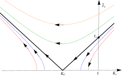
Figure 14: Renormalization-group flows for resonant tunneling in TIs for $1<g<2$, given by Eq. (57). The different lines indicate different initial parameter $t_{0}$; the RG flows always starts from $K_{s}=1$. The thick dashed line represents the separatrix, which is of the Kosterlitz-Thouless universality class. When $t_{0}$ is larger than $t_{*},$ the system flows to the conducting phase, while for $t_{0}$ smaller than $t_{*}$, the system flows to the insulating phase. This plot is made at $g=1.05$.

If $\alpha$ is a constant, we can divide Eq. (52) by (56) and integrate to obtain

$$\tilde{t}_{{}_{c}}^{2}=t_{0}^{2}+\frac{\left(K_{s}-1\right)g^{2}}{1+\alpha g^{2}}-\frac{2g-1}{1+\alpha g^{2}}\ln K_{s}.$$ (57)

where $t_{0}=\tilde{t}_{{}_{c}}(l=0)$ is the bare value of the tunneling. Fig. 14 show a plot of this solution for various different parameters $t_{0}$. From the plot, the strategy to find the critical $t_{0}\equiv t_{*}$ is clear. If $\tilde{t}_{{}_{c}}^{2}$ remains positive, then the eventual fixed point of the flow will be $K=0$, $\tilde{t}_{{}_{c}}\rightarrow\infty$; while if $\tilde{t}_{{}_{c}}^{2}=0$ anywhere along the flow line, then this is the fixed point (a similar situation occurs in the Kosterlitz-Thouless phase diagram).

By differentiating, we find that the minimum value of $\tilde{t}_{{}_{c}}^{2}$ occurs at a value

$$K_{c}=\frac{2}{g}-\frac{1}{g^{2}}.$$ (58)

The critical $t_{*}$ is therefore given by the solution to the equation $\tilde{t}_{{}_{c}}^{2}(K_{c})=0$; executing the calculation yields

$$t_{*}^{2}=\frac{\left(g-1\right)^{2}}{1+\alpha g^{2}}+\frac{2g-1}{1+\alpha g^{2}}\ln\left[1-\left(\frac{g-1}{g}\right)^{2}\right].$$ (59)

In the vicinity of $g=1+\varepsilon$ with $\varepsilon\ll 1$, expanding (59) gives

$$\frac{\varepsilon^{4}}{2(1+\alpha_{\mathrm{max}})}<t_{*}^{2}<\frac{\varepsilon^{4}}{2}.$$ (60)

Assuming that all bare tunneling amplitudes are equal so $\alpha_{\textrm{max}}=1$, this gives the condition in Eq. (28) quoted in the main text. These bounds, along with a numerical determination of the phase boundary are shown in Fig. 6.

We now discuss briefly how the phase boundary is affected if the quadratic terms in Eq. (27) are included, i.e. if we set $A\neq 0$. In the vicinity of $g=1$ where the linear terms may be zero, it is not a priori obvious that one can ignore the quadratic terms. However, the fact that the phase boundary line approaches zero as $\varepsilon^{2}$ means that in the vicinity of the transition line, such terms are of order $\varepsilon^{4}$ while the first term behaves as $\varepsilon^{3}$. We therefore conclude that including the quadratic terms does not significantly affect the phase boundary – this is also backed up by the numerical plot of the phase boundary at $A=1$ in Fig. 6.

Appendix C Analytical analysis of the RG flow

In this appendix, we analyse the flow of Eqs. (27) as a function of $l$ in order to locate $l^{*}$ and $l_{K}$, corresponding through the relation $l=\ln(\Lambda/T)$ to the minimum-conductance temperature and Kondo temperature respectively. Our goal will be parametric relations when the bare parameters are small, hence we will ignore the quadratic terms (i.e. set $A=0$), which means that as usual, the equation for $t_{{}_{e}}$ decouples, and we can ignore it. The initial conditions are that $\tilde{t}_{{}_{c}}(l=0)=\tilde{t}_{{}_{s}}(l=0)=t_{0}$ and $K_{s}(l=0)=1$.

We begin by noticing that we can write the formal solution to Eq. (27b) as

$$\tilde{t}_{{}_{c}}(l)=t_{0}\exp\left[(1-1/2g)l-\frac{g}{2}\int_{0}^{l}K_{s}(l^{\prime})dl^{\prime}\right].$$ (61)

By substituting this into Eq. (27d) and further using (55), we find that

$$\frac{1}{K_{s}}\frac{dK_{s}}{dl}=\\ -t_{0}^{2}\left[\frac{e^{(2-1/g)l}}{g}+ge^{(2-g)l}\right]\exp\left[-g\int_{0}^{l}K_{s}(l^{\prime})dl^{\prime}\right].$$ (62)

Now initially, the flow of $K_{s}$ is close to one, so approximating $K_{s}$ on the RHS of (62) by $1$, we can integrate to obtain

$$K_{s}(l)=\exp\left\{-t_{0}^{2}\left[\frac{e^{(2-g-1/g)l}-1}{g(2-g-1/g)}+\frac{g(e^{(2-2g)l}-1)}{2-2g}\right]\right\}.$$ (63)

where we have additionally taken $g\neq 1$. This expression is fine until $K_{s}$ starts differing significantly from $1$. In particular, we can use it until the scale $l^{*}$ defined by $K_{s}(l^{*})=K_{c}$ with $K_{c}$ given in Eq. (58). This is exactly the scale at which $\tilde{t}_{{}_{c}}(l)$ takes a minimum value, and is given by the solution of

$$\frac{e^{(2-g-1/g)l^{*}}-1}{g(2-g-1/g)}+\frac{g(e^{(2-2g)l^{*}}-1)}{2-2g}=\frac{\ln(g^{2}/(2g-1))}{t_{0}^{2}}.$$ (64)

It is worth pointing out that if $g>1$, then the two terms on the left hand side are exponentially decaying, and therefore this equation may not have a solution with $l^{*}>0$ if $t_{0}$ is too small. This is an alternative way of looking at the phase transition.

Limiting ourselves to parameters where there is a solution, writing $g=1+\varepsilon$ and expanding in small $\varepsilon$ gives expression (30) in the main text. Assuming $g<1$, the second term on the LHS of (64) is exponentially growing and therefore dominant; by taking the leading behavior and ignoring prefactors gives expression (31) in the main text. Substituting this value of $l^{*}$ into (61) (and again approximating $K_{s}=1$ on the RHS) gives Eq. (32) in the main text.

Now, for $l>l^{*}$, we can no longer approximate $K_{s}$ as $1$. However for $g<1$ (or more formally $(1-g)/t_{0}\gg 1$), we can make progress. In this limit, due to the exponentially increasing term on the RHS of (63), we see that $K_{s}$ drops very rapidly to become close to zero. Hence to leading order, we can say that

$$\int_{0}^{l>l^{*}}K_{s}(l^{\prime})dl^{\prime}\approx l^{*},$$ (65)

and hence from (61) we obtain

$$\tilde{t}_{{}_{c}}(l>l^{*})=t_{0}\exp\left[(1-1/2g)l-gl^{*}/2\right].$$ (66)

Solving this to find the scale where $t_{{}_{c}}(l_{K})=1$ gives expression (33) in the main text, while the flow of $\tilde{t}_{{}_{c}}$ between $l^{*}$ and $l_{K}$ gives the intermediate-scale power-law quoted in the main text.

For $g>1$, the approximations leading to the results about $T_{K}$ no longer are valid – the lack of an exponentially increasing factor in Eq. (63) means that the deviation of $K_{s}$ from one in the RHS of Eq. (62) is crucial. In fact, looking at numerical results, one can see that in this case, the decrease in $K_{s}$ from $1$ to $0$ happens exactly over the same energy region as $\tilde{t}_{{}_{c}}$ flows to strong coupling. This intertwining of energy scales means that there is no great separation in scale of $T^{*}$ and $T_{K}$, and hence the intermediate regime in the pictures may be rather narrow. We therefore say no more about this region here.

References

- Prange and Girvin (1990) R. Prange and S. M. Girvin, eds., The Quantum Hall Effect (Springer-Verlag, New York, 1990).
- Das Sarma and Pinczuk (1997) S. Das Sarma and A. Pinczuk, eds., Perspectives in Quantum Hall Effects (John Wiley & Sons, INC., 1997).
- Hasan and Kane (2010) M. Z. Hasan and C. L. Kane, Rev. Mod. Phys. 82, 3045 (2010).
- Qi and Zhang (2011) X.-L. Qi and S.-C. Zhang, Rev. Mod. Phys. 83, 1057 (2011).
- Kane and Mele (2005) C. L. Kane and E. J. Mele, Phys. Rev. Lett. 95, 226801 (2005).
- Bernevig and Zhang (2006) B. A. Bernevig and S.-C. Zhang, Phys. Rev. Lett. 96, 106802 (2006).
- Bernevig et al. (2006) B. A. Bernevig, T. L. Hughes, and S.-C. Zhang, Science 314, 1757 (2006).
- König et al. (2007) M. König, S. Wiedmann, C. Brune, A. Roth, H. Buhmann, L. W. Molenkamp, X.-L. Qi, and S.-C. Zhang, Science 318, 766 (2007).
- Levin and Stern (2009) M. Levin and A. Stern, Phys. Rev. Lett. 103, 196803 (2009).
- Neupert et al. (2011) T. Neupert, L. Santos, C. Chamon, and C. Mudry, Phys. Rev. Lett. 106, 236804 (2011).
- Levin and Stern (2012) M. Levin and A. Stern, Phys. Rev. B 86, 115131 (2012).
- Oreg et al. (2013) Y. Oreg, E. Sela, and A. Stern, ArXiv e-prints (2013), eprint 1301.7335.
- Xu and Moore (2006) C. Xu and J. E. Moore, Phys. Rev. B 73, 045322 (2006).
- Wu et al. (2006) C. A. Wu, B. A. Bernevig, and S.-C. Zhang, Phys. Rev. Lett 96, 106401 (2006).
- Maciejko et al. (2009) J. Maciejko, C. Liu, Y. Oreg, X.-L. Qi, C. Wu, and S.-C. Zhang, Phys. Rev. Lett. 102, 256803 (2009).
- Schmidt et al. (2012) T. L. Schmidt, S. Rachel, F. von Oppen, and L. I. Glazman, Phys. Rev. Lett. 108, 156402 (2012).
- Lezmy et al. (2012) N. Lezmy, Y. Oreg, and M. Berkooz, Phys. Rev. B 85, 235304 (2012).
- Budich et al. (2012) J. C. Budich, F. Dolcini, P. Recher, and B. Trauzettel, Phys. Rev. Lett. 108, 086602 (2012).
- Goth et al. (2013) F. Goth, D. J. Luitz, and F. F. Assaad, ArXiv e-prints (2013), eprint 1302.0856.
- Büttiker (1988) M. Büttiker, Phys. Rev. B 38, 9375 (1988).
- Giamarchi (2003) T. Giamarchi, Quantum physics in one dimension (Oxford University Press, 2003).
- Kane and Fisher (1992a) C. L. Kane and M. P. A. Fisher, Phys. Rev. B 46, 15233 (1992a).
- Teo and Kane (2009) J. C. Y. Teo and C. L. Kane, Phys. Rev. B 79, 235321 (2009).
- Hou et al. (2009) C.-Y. Hou, E.-A. Kim, and C. Chamon, Phys. Rev. Lett. 102, 076602 (2009).
- Ström and Johannesson (2009) A. Ström and H. Johannesson, Phys. Rev. Lett. 102, 096806 (2009).
- Liu et al. (2011) C.-X. Liu, J. C. Budich, P. Recher, and B. Trauzettel, Phys. Rev. B 83, 035407 (2011).
- Wen (1991) X.-G. Wen, Phys. Rev. B 44, 5708 (1991).
- Kane and Fisher (1992b) C. L. Kane and M. P. A. Fisher, Phys. Rev. B 46, 7268 (1992b).
- Lee and Toner (1992) D.-H. Lee and J. Toner, Phys. Rev. Lett. 69, 3378 (1992).
- Furusaki and Nagaosa (1993a) A. Furusaki and N. Nagaosa, Phys. Rev. B 47, 4631 (1993a).
- Furusaki and Nagaosa (1993b) A. Furusaki and N. Nagaosa, Phys. Rev. B 47, 3827 (1993b).
- de C. Chamon and Wen (1993) C. de C. Chamon and X. G. Wen, Phys. Rev. Lett. 70, 2605 (1993).
- Gogolin et al. (1998) A. O. Gogolin, A. A. Nersesyan, and A. M. Tsvelik, Bosonization and strongly correlated systems (Cambridge University Press, 1998).
- Rajaraman (1982) R. Rajaraman, Solitons and instantons: an introduction to solitons and instantons in quantum field theory (North-Holland, 1982).
- Law et al. (2010) K. T. Law, C. Y. Seng, P. A. Lee, and T. K. Ng, Physical Review B 81, 041305(R) (2010).
- Seng and Ng (2011) C. Seng and T. K. Ng, Europhys. Lett. 96, 67002 (2011).
- Chung and Silotri (2012) C.-H. Chung and S. Silotri, ArXiv e-prints (2012), eprint 1201.5610.
- Eriksson et al. (2012) E. Eriksson, A. Ström, G. Sharma, and H. Johannesson, Phys. Rev. B 86, 161103 (2012).
- Posske et al. (2013) T. Posske, C.-X. Liu, J. C. Budich, and B. Trauzettel, Phys. Rev. Lett. 110, 016602 (2013).
- Lee and Lee (2013) Y.-L. Lee and Y.-W. Lee, ArXiv e-prints (2013), eprint 1303.1896.
- Chao et al. (2013) S.-P. Chao, S. A. Silotri, and C.-H. Chung, ArXiv e-prints (2013), eprint 1305.2563.
- Eriksson (2013) E. Eriksson, Phys. Rev. B 87, 235414 (2013).
- Maslov and Stone (1995) D. L. Maslov and M. Stone, Phys. Rev. B 52, R5539 (1995).
- Ponomarenko (1995) V. V. Ponomarenko, Phys. Rev. B 52, R8666 (1995).
- Safi and Schulz (1995) I. Safi and H. J. Schulz, Phys. Rev. B 52, R17040 (1995).
- Wen (1990) X. G. Wen, Phys. Rev. B 41, 12838 (1990).
- Wen (1992) X.-G. Wen, Int.J.Mod.Phys. B6, 1711 (1992).
- Beri and Cooper (2012) B. Beri and N. R. Cooper, Phys. Rev. Lett. 108, 206804 (2012).
- Schmid (1983) A. Schmid, Phys. Rev. Lett. 51, 1506 (1983).
- Saleur (1999) H. Saleur, in Topological Aspects of Low Dimensional Systems, edited by A. Comtet, T. Jolicoeur, S. Ouvry, and F. David (1999), p. 473.
- Glazman and Raikh (1988) L. I. Glazman and M. E. Raikh, JETP Lett. 47, 452 (1988).
- Ng and Lee (1988) T. K. Ng and P. A. Lee, Phys. Rev. Lett. 61, 1768 (1988).