Complementarity and Classical Limit of Quantum Mechanics: Energy Measurement aspects

Abstract

In the present contribution we discuss the role of experimental limitations in the classical limit problem. We studied some simple models and found that Quantum Mechanics does not re-produce classical mechanical predictions, unless we consider the experimental limitations ruled by uncertainty principle. We have shown that the discrete nature of energy levels of integrable systems can be accessed by classical measurements. We have defined a precise limit for this procedure. It may be used as a tool to define the classical limit as far as the discrete spectra of integrable systems are concerned. If a diffusive environment is considered, we conclude that the ”lifetime” of discreteness is approximately $1/\kappa$ ($\kappa$ is the diffusion constant), thus it was possible to relate the classical limit of a spectra with the action of an environment and experimental resolution.

I Introduction

Since the early twentieth century, the predictions of quantum mechanics were strange to most people and almost always seemed to contradict our common sense. There were no conclusive explanation for the disappearance of quantum effects in the macroscopic regime. Which of the quantum features we don’t see in our day life experience? One of the most disconcerting one is the wave-particle duality. This is in fact the first quantum feature that has a strong argument explaining its disappearance in the macroscopic world. The solution is in de Broglie expression for the wavelength. The length of the wave interference fringes becomes insignificant as we increase the classical action of the system. There are many other quantum features that are unobservable in the macroscopic regime, such as entanglement and discreteness of energy spectrum. Other important open question is about the classical regime. Does quantum mechanics reproduce the observed results of macroscopic experiments? The first try to answer this question is attributed to Bohr, the correspondence principle. Bohr’s correspondence principle Bohr :

”Indeed, as adequate as the quantum postulates are in the phenomenological description of the atomic reactions, as indispensable are the basic concepts of mechanics and electrodynamics for the specification of atomic structures and for the definition of fundamental properties of the agencies with which they react. Far from being a temporary compromise in this dilemma, the recourse to essentially statistical considerations is our only conceivable means of arriving at a generalization of the customary way of description sufficiently wide to account for the features of individuality expressed by the quantum postulates and reducing to classical theory in the limiting case where all actions involved in the analysis of the phenomena are large compared with a single quantum. In the search for the formulation of such a generalization, our only guide has just been the so called correspondence argument, which gives expression for the exigency of upholding the use of classical concepts to the largest possible extent compatible with the quantum postulates.”

Bohr also stated the postulate known as selection rule:

”This peculiar relation suggests a general law for the occurrence of transitions between stationary states. Thus we shall assume that even when the quantum numbers are small the possibility of transition between two stationary states is connected with the presence of a certain harmonic component in the motion of the system Bohr1920 . ”

Bohr’s correspondence principle and his selection rule were later interpreted as Home :

1. “Quantum mechanical predictions must correspond to classical ones in the limit of large quantum numbers.”

2. “A selection rule must be valid for all possible quantum numbers. Thus, a selection rule must be valid for classical and quantum regimes.”

The Correspondence Principle of Quantum Mechanics is a widely used tool to study quantum to classical transition problem since its conception by Bohr Bohr1920 ; Bohr . Nevertheless, Quantum and Classical Mechanics are incommensurable theories because their basic ontologies are different. The basic entities of Classical Mechanics (CM) are coordinates and velocities in configuration spaces. Quantum Mechanics (QM) deals with state vectors and operators in Hilbert space Laloe . Since both theories give acceptable descriptions of different experiments in limiting situations there should be a way of translating their predictions from one to the other, in going from QM to CM this is the so called classical limit problem Zur1996 . There are also attempts to explain experimental results usually in quantum domain within the framework of CM Rubin ; Luca ; Figueiredo ; Gesil .

In the core of the Correspondence Principle there are two “beliefs” that has influenced the study of the classical limit problem. The first one is that classical mechanics is able to reproduce macroscopic experimental observations within an arbitrary precision in a such way that its predictions can be used for comparison with the quantum description of the experiment. The second one is that “typical quantum objects” and “typical classical objects” are subjected to the same conditions. Although the confirmation of these “beliefs” may be desirable, this is not necessary nor sufficient. We know that an experimental result, usually in classical domain, can be considered as a quantum one Yu02 ; Inomata05 . This problem can be extended to a more general problem of comparing two theories. Suppose we have two theories A and B, and that it is common sense that theory A has a validity domain that includes the domain of B, i.e., A $\supset$ B. Thus, it is expected that theory A reproduces all the results for B and it should also not be in contradiction with theory B in its domain. A typical example is special relativity, where we adopt slow velocity limit to yield Newtonian regime. Strictly speaking about classical mechanics, some points are relevant to our discussion:

1. Classical mechanics is a very successful theory, but it does not mean that there is no uncertainty within its predictions. Inaccuracies are unavoidable, but in classical domain Newtonian dynamics is in agreement with the observations.

2. It would be very interesting to obtain classical mechanics from quantum mechanics in terms of a limit, such as high energy or mass. Although that, the parameter to be used should not be a universal constant such as $\hbar$. For practical reasons it should be a variable that can be manipulated in a laboratory.

3. There is not a known experimental criteria of general validity which determines if a quantum state can be considered classical in all aspects or all possible measurements.

The above comments take us to philosophical questions, such as what is the objective of a physical theory? What do we need to build a useful theory? Which criteria one should use to compare two theories? It is common sense that a good physical theory must reproduce the experimental results within the error bar. It would be more acceptable if it is able to predict unknown phenomena. A physical theory must include mathematical entities which the physicist should associate with the ones observed in laboratory. With the help of such mathematical entities, one should be able to predict the time evolution of the observed physical entities. The last question is a subject of a stronger debate Zur1996 ; Ball98 ; Ball01 ; Oliveira02 ; Dalvit ; Wiebe ; Oliveira06 ; Faria07 ; Davidov ; Bosco ; adelcio2012 ; Gabi ; renato2007 . If it was always possible to measure the quantum state, it would be a most precise separability criteria. But in fact we know how to measure Wigner functions only in some specific situations Lutter1 ; Lutter2 ; Davidov ; Banaszek ; Mukamel ; Kenfack ; Toscano06 . Let us go back to the general problem of theories A and B. Suppose that an experimentalist makes an experiment in B domain, and the result is compatible, within experimental error bar, with theory B. If theory A also gives a good description of the experiment and its prediction is in accordance with the results, we can thus say that for this specific experiment both theories are satisfactory, meaning that they are equivalent for this case. If $Im(A)\bigcap$Im(B)$\neq\emptyset$, it is possible to have such an experimental result compatible with theories A and B: in this sense, the theories are not divergent. Due to the experimental errors Rajeev ; adelcio2012 , or inaccuracies , that are unavoidable and inherent to quantum theory, a point in domain should be represented as a volume in its image. If all possible realizable experiments in B domain have their image in the intersection of theories image we can thus say that theory A successfully replaces B.

The investigation of the correspondence principle employing a quartic oscillator coupled to a diffusive phase reservoir and taking into account the limited experimental resolution is found in Ref. renato2007 ; adelcio2012 . They studied the system dynamics in perspective of an observable, the position or momentum.

In ref. adelcio2012 they show that the problem of the quantum-to-classical transition is close related to decoherence and inaccuracies of measurements on the correspondence of the two descriptions. They claimed that isolated systems and measurements with unlimited accuracy are mere idealizations.

In this contribution, the main goal is to investigate the role of experimental errors and of environment in the quantum-classical transition problem. We focuss on the spectra discreteness. We propose a heuristic procedure (not deduced mathematically within the theory) to use spectroscopic information from model Hamiltonians and time energy Heisenberg relations in order to decide whether a quantum system can be described by CM. The quantum behavior is characterized by the discreteness of energy spectra. We are considering a gedankenexperiment, where the experimentalist does not know Quantum Mechanics but tries obtain the energy spectrum. Will he be able to conclude that it is discrete?

II
The large quantum numbers limit

One controversial subject in quantum mechanics is the time-energy uncertainty relation ($\Delta t.\Delta E\geq\frac{\hbar}{2}$) and it is not our aim to bring this discussion to the present work. Nevertheless it is well known that time and frequency are conjugated variables in a pair of Fourier transforms in classical physics, the duration of a signal and the respective frequency are subjected to an unsharpness relation ($\Delta t.\Delta\omega\geq\frac{1}{2}$) that is classical indeed. Frequency, in quantum theory, is another way of speaking about energy. An uncertainty relation between time and energy must be seriously considered, studied and interpreted, although there are objections due to the fact that time is not associated to a dynamical operator canonically conjugated to the hamiltonian. An exhaustive examination of this matter is made by Peres in his book Peres 2002 . On the other hand we have to assume that QM is not an objective description of physical reality. It only predicts the probability of occurrence of stochastic macroscopic events, following specified preparation procedures. These predictions are based on conceptions that are given to know indirectly - like all the microscopic elements as electrons, photons, etc. They have no substance at all, they are just perceived or understood by their interactions with measurement devices. We want to avoid these interpretational intricacies of QM by stating the problem in another way: how to describe the aim of measurement or what  has actually to be done in a measurement process?

The main stream of our proposal is not face the discussion of the time-energy uncertainty relation, we face the problem of to decide under what conditions a system may be considered as Classical or Quantum. It is in this sense that we tackle the problem of dealing with the physical reality: how can one measure and what is in fact measured. Thus, we use the product of energy differences between neighbour levels by the corresponding classical period differences to compare with the time-energy uncertainty relation to classify a system as classical or quantum. If this product fulfills the time-energy uncertainty relation it is quantum otherwise it is classical.

To do this we add an element connected to this subject that concerns integrable systems: the decision wether a system is classical or quantum depends on the experimental apparatus which are essentially classical. One undoubtedly quantum feature is the discreteness of at least part of the energy spectrum. The essential idea here is that if one tries to measure the energy of the system in question using classical canonical pairs $q$, $p$, the information about the quantum nature of the particle will be lost. In spite of this fact, as we show in what follows, the function

$$y(n)=\left|\Delta E_{n}\Delta\tau_{n}\right|$$ (1)

where $\Delta E_{n}=\left(E_{n}-E_{n-1}\right)/2$ is merely the energy difference between two neighbour levels, (it is the maximum uncertainty in energy for the state $a\left|E_{n}\right\rangle+b\left|E_{n-1}\right\rangle$ ) and $\Delta\tau_{n}=\left(\tau_{n}-\tau_{n-1}\right)/2,$ with $\tau_{n}$ being the classical period associated to the energy $E_{n}.$ If the experiment has an accuracy $\delta t$ it limits the period measurement precision, in real systems it is desirable that $\delta t<<\Delta\tau$, we assume that they are of same order, $\Delta\tau\approx$ $\delta t.$

The $y(n)$ function can be heuristically justified if we consider the Bohr-Sommerfeld quantization rule for periodic systems, that states

$$I=\oint pdq=2\pi\hbar n$$ (2)

thus we have

$$\left\langle K\right\rangle=\frac{\pi n\hbar}{\tau},$$ (3)

where $\left\langle K\right\rangle$ is the the mean kinetic energy, $\tau$ being the classical period associated with $K$ and $n$ is a quantum number. Observing that Darrigol

$$\delta I=\oint\delta Hdt$$ (4)

Consider two neighboring periodic motions of the same system. Then H is a constant, and we have

$$\delta I=\tau\delta H.$$ (5)

Note that (5) determines that the energy of the system depends only on I, then Bohr’s quantiztion rule determines the energy of the system, for more detail see Darrigol .

The Bohr-Sommerfeld quantization rule makes a direct conection between kinetics energy and classical period, it was also demonstrated adelcioJMP that, for integrable systems, is possible to reconstruct semiclassicaly the quantum state using classical dynamics. Since you know the Wigner function of the system it is possible to infer the period related to the state adelcioJMP ; Oliveira01 .

Alternatively, we can use the semiclassical quantization rule Berryi ; Stockmann for integrable systems, we have a similar result Stockmann ; Wisniacki ; Novaes .

This function (1) is stated for a more clear definition of a classical limit. As we will show, the fact that one will only be able to see a continuum of energies does not mean that the classical limit has been reached. It only reveals that we have become “myope” to see the nature of the spectrum.

In what follows, we will consider a simple one dimensional systems with discrete spectra. Let us assume that a state has been prepared in the following way

$$\left|\Psi(0)\right\rangle=a\left|E_{n}\right\rangle+b\left|E_{n-1}\right\rangle$$ (6)

where $\left\{\left|E_{n}\right\rangle\right\}$ are eigenstates of the hamiltonian $H$

$$\hat{H}\left|E_{n}\right\rangle=E_{n}\left|E_{n}\right\rangle$$ (7)

The variance in energy difference, for any time, of this state is given by

$$\Delta E=\left|a\right|\left|b\right|\left[E_{n}-E_{n-1}\right]$$ (8)

Using the normalization condition $\left|a\right|^{2}+\left|b\right|^{2}=1$, it is easy to check that the maximum for this energy difference is achieved for $\left|a\right|=\left|b\right|=1/\sqrt{2}$, and is given by

$$\Delta E(n)=1/2\left|E_{n}-E_{n-1}\right|.$$ (9)

How do we define the classical limit in this simple case? Let us assume the following $\displaystyle\lim_{n\rightarrow\infty}\frac{\Delta E_{n}}{E_{n}}=0$.

The above expression means that as the energy increases $(E_{n})$, the uncertainty in energy of the state $\left|\Psi(t)\right\rangle$ becomes negligible as compared to $E_{n}.$ Let us discuss a few examples.

Harmonic Oscillator

For the harmonic oscillator we have

$$\Delta E=\frac{1}{2}\hbar\omega\Longrightarrow\frac{\Delta E}{E_{n}}=\frac{1/2}{(n+1/2)}$$ (10)

and we clearly have $\displaystyle\lim_{n\rightarrow\infty}\frac{\Delta E_{n}}{E_{n}}=0$.

Particle in a box

In this case we have

$$E_{n}=\hbar^{2}\frac{n^{2}\pi^{2}}{2ma^{2}},$$ (11)

where $n=1,2,3,dots$, $m$ is the mass of the particle and $a$ is the box width. Then we have

$$\Delta E_{n}=\hbar^{2}/4\left|\frac{(2n-1)\pi^{2}}{ma^{2}}\right|.$$ (12)

Once again we have $\lim_{n\rightarrow\infty}{\displaystyle{\frac{\Delta E_{n}}{E_{n}}}}\rightarrow 0.$

The fact that this limit is zero is the argument usually found in textbooks in order to define the classical limitHome ; Cohen ; Eisberg . Of course it is true that when one considers the high energy limit, it becomes increasingly difficult to obtain good experimental resolution. However, as we show below, this limit does not necessarily imply that it is impossible to obtain the needed resolution. As we know, quantization has been observed in some macroscopic systems like superconducting Josephson junctions Richard . Besides, one can use something analogous to the Heisenberg microscope Quantummesurement in order to obtain the velocity of the particle. In the case of a particle in a box, discussed above, once we know the velocity, the energy is easily obtained. The measurement of the velocity implies a perturbation of the position which depends on the characteristics of the apparatus and in principle, is independent of the quantum number $n$. Thus, if one uses the adequate measurement the discrete character of a spectrum can be verified.

III Classical measurement of the Energy

When one deals with realistic systems, say, atoms, the spectrum is obtained from the emitted or absorbed electromagnetic radiation. A completely different approach is used for macroscopic systems. Within CM, for closed systems, the energy is a function of position and momentum $E=f(p,q).$ So, from now on, we will call Classical Measurement of energy every process which makes use of the relation $E=f(p,q)$ in order to obtain the energy of a given system, classical or quantum. As an example, we may look at the particle in a box again. In this case, the energy is a direct function of the velocity, so that once we determine de velocity, the energy will be defined. In practice, one may measure the time it takes for $2s$ inversions in the momentum and so determine the period of the motion . Classically, the period is given by

$$\tau=\frac{2a}{v}=a\sqrt{\frac{2m}{E}.}$$ (13)

In the above expression, we are considering the correspondent classical period for a specific energy eigenvalue. Since the energy levels are determined by QM, regardless of the energy scale one is talking about, the allowed values of the period are

$$\tau_{n}=\frac{2a^{2}m}{\hbar n\pi}.$$ (14)

So, the difference in period for two quantum neighboring levels is

$$\Delta\tau=\frac{\tau_{n}-\tau_{n-1}}{2}=-\frac{a^{2}m}{\hbar\pi}\frac{1}{\left(n-1\right)n}.$$ (15)

From the above expression one can see that it becomes increasingly difficult to distinguish two higher adjacent energy levels by this method. Let us take a look at the product $\left|\Delta E_{n}\Delta\tau_{n}\right|$ where $\Delta E_{n}=\left(E_{n}-E_{n-1}\right)/2$ and $\Delta\tau_{n}=\left(\tau_{n}-\tau_{n-1}\right)/2.$ $\tau_{n}$ is the classical period associated with the energy $E_{n}.$ It is interesting to observe the behavior of the function

$$y(n)=\left|\Delta E_{n}\Delta\tau_{n}\right|.$$ (16)

For the case in question,

$$y(n)=\frac{\hbar\pi}{4}\frac{(2n-1)}{\left(n-1\right)n}.$$ (17)

If we take $n=4,$ we find $y(4)<\hbar/2$, which means that we won’t have enough precision to verify whether the spectrum is discrete or continuous, since Quantum Mechanics forbids such precision. Here, we are just using the fact that the time-energy uncertainty relation has to be respected since we are considering that Quantum Mechanics must prevent Classical Mechanics. Also it is easy to see that $\displaystyle\lim_{n\rightarrow\infty}y(n)=0.$

In the more realistic case of a hydrogenoid atom we have

$$E_{n}=-\frac{\mu Z^{2}e^{4}}{2\hbar^{2}n^{2}}$$ (18)

where $Ze$ is the total charge interacting with the electron of charge $e$, and $\mu$ is the reduced mass of the system. As opposed to the previous case, the energy levels become closer as $n$ grows. Thus, the question is: from which $n$ can we say that the spectrum is continuous from the point of view of Classical Mechanics? In this case

$$\Delta E=\frac{\mu Z^{2}e^{4}}{4\hbar^{2}}\left|\frac{2n-1}{n^{2}(n-1)^{2}}\right|,$$ (19)

$$\Delta T=\frac{\pi\hbar^{3}}{Z^{2}e^{4}\mu}\left[3n^{2}-3n+1\right],$$ (20)

and

$$y(n)=\frac{\pi\hbar\left(2n-1\right)\left[3n^{2}-3n+1\right]}{4n^{2}(n-1)^{2}}.$$ (21)

Now, for the $1/r$ potential, we have $y(n)<\hbar/2$ for $n=9$, so one won’t be able to observe the quantization for $n$ bigger than 9 while using classical measurement of the energy.

Other interesting case is the Morse Potential, frequently used to describe the spectra of molecules Oliveira01 . The Morse potential is defined as

$$U(x)=D\left(e^{-2\alpha x}-2e^{-\alpha x}\right),$$ (22)

where $D$ and $\alpha$ are constants experimentally determined. For $s$ waves, i.e., the orbital angular momentum is zero, we have

$$E(n)=-D+\hbar\omega\left[\left(n+1/2\right)-\frac{1}{\zeta}\left(n+1/2\right)^{2}\right].$$ (23)

$\zeta$ is also experimentally determined. The classical period corresponding to each $E(n)$ is given by

$$\tau(n)=2\pi\sqrt{\frac{MRo^{2}}{2\left|E(n)\right|\alpha^{2}}}$$ (24)

where $Ro$ is a function of $\alpha$ and $\zeta.$ It is easy to verify that, for the hydrogen molecule parameters, $y(n)<\hbar/2$ for all possible $n$. Since the Morse potential is quasi-harmonic for low energies we observe that it is not possible to distinguish neighboring discrete states with a classical measurement. From this example, we may conclude that any potential that is approximately harmonic have no assessable discrete spectrum through a classical measurement of the energy.

III.1 Harmonic Oscillator

For a harmonic oscillator, $E=\frac{p^{2}}{2m}+\frac{1}{2}kq^{2}$ , its period is $\tau=\frac{2\pi}{\omega}$ where $\omega=\sqrt{\frac{k}{m}}$ which is energy independent, thus we conclude that it can not be used to characterize the spectrum. Another way of classically determining the energy can be obtained by measuring q and p at same time, therefore classical energy uncertain is given by

$$\delta E=\frac{p}{m}\delta p+kq\delta q$$ (25)

Without lost of generality, we choose $\delta p=\sqrt{\frac{m\hbar\omega}{2}}a$ and $\delta q=\sqrt{\frac{\hbar}{2m\omega}}a$ then we obtain the relation

$$\delta p\delta q=a^{2}\hbar/2.$$ (26)

In case of a=1 we have the minimum uncertain defined under Hisenberg relation, in general we have

$$\delta E=\left[|p|\sqrt{\frac{\hbar\omega}{2m}}+k|q|\sqrt{\frac{\hbar}{2m\omega}}\right]a$$ (27)

then

$$\delta E^{2}=\frac{2}{\hbar}\left[p\sqrt{\frac{\hbar\omega}{2m}}+kq\sqrt{\frac{\hbar}{2m\omega}}\right]^{2}\delta p\delta q$$ (28)

From (10) we have

$$\delta E=\frac{1}{2}\hbar\omega$$ (29)

thus we find

$$\delta p\delta q=\frac{\hbar^{3}\omega^{2}}{4\left[|p|\sqrt{\frac{\hbar\omega}{2m}}+k|q|\sqrt{\frac{\hbar}{2m\omega}}\right]^{2}}.$$ (30)

Note that

$$\left[|p|\sqrt{\frac{\hbar\omega}{2m}}+k|q|\sqrt{\frac{\hbar}{2m\omega}}\right]^{2}=\left(\frac{p^{2}}{2m}+\frac{1}{2}kq^{2}+|pq|\omega\right)\hbar\omega,$$ (31)

if we consider the energy as $E=\hbar\omega(n+1/2)$, we find

$$\delta p\delta q=\frac{\hbar^{2}}{4\left(\hbar(n+1/2)+|pq|\right)}$$ (32)

From (32) we see that we need an experimental resolution that is avoided by Quantum Mechanics. Thus we can say that his spectrum can not be resolved by Classical Energy Measurement.

IV Neighbors Distinguishability

Let us consider a quartic oscillator model. Its Hamiltonian is

$$\hat{H}_{0}=\hbar\omega\hat{a}^{\dagger}\hat{a}+\lambda\hbar^{2}(\hat{a}^{\dagger}\hat{a})^{2}$$ (33)

where $\hat{a}$ and $\hat{a}^{\dagger}$ are destruction and creation operators of the harmonic oscillator, $\omega$ is the natural frequency of the main oscillator, $\lambda$ is the non-linear strength constant. The system has as energy levels

$$E(n)=\hbar\omega n+\lambda\hbar^{2}n^{2}.$$ (34)

Its classical counterpart, with an energy given by (34) has a period given by

$$\tau=\frac{2\pi}{\omega+2\lambda\hbar n},$$ (35)

then we have

$$y(n)=\frac{\pi\lambda\hbar^{2}\left[\omega+\lambda\hbar(2n-1)\right]}{\left[\omega+2\lambda\hbar(n-1)\right]\left[\omega+2\lambda\hbar n)\right]}.$$ (36)

The case $\lambda\hbar\ll\omega$ we obtain harmonic potential, as expected, and for $\lambda\hbar\gg\omega$ we obtain the infinity well result:

$$\lim_{\lambda\hbar/\omega\rightarrow 0}y(n) \approx \frac{\pi\lambda\hbar^{2}}{\omega},$$ (37)

$$\lim_{\lambda\hbar/\omega\rightarrow\infty}y(n) \approx \frac{\pi\hbar(2n-1)}{4(n-1)n}.$$ (38)

Considering $\lambda\hbar\gg\omega,$ in principle we can access the discreet spectra for $n<4$.

Up to now, we didn’t consider the environment action. Real systems are never isolated, thus in a real experiment we can not ignore its action. Due to the impossibility of modeling the system and its surrounding from first principles, we are forced to treat the environment as a collection of harmonic oscillators, as usual Isar . We use the model of the quartic oscillator Oliveira02 ; Oliveira06 ; renato2006 ; renato2007 ; Faria07 ; Greiner ; Agarwal coupled to a bath of harmonic oscillators. This model is described by the hamiltonian

$$\hat{H}_{q}=\hat{H}_{0}+\hat{H}_{int}+\hat{H}_{A}$$ (39)

where

$$\hat{H}_{0}=\hbar\omega\hat{a}^{\dagger}\hat{a}+\lambda\hbar^{2}(\hat{a}^{\dagger}\hat{a})^{2}$$ (40)

is the hamiltonian that governs the free evolution of the system of interest,

$$\hat{H}_{A}=\sum_{k}\hbar\omega_{k}\hat{b}_{k}^{\dagger}\hat{b}_{k}$$ (41)

is the hamiltonian that governs the free evolution of the set of environmental harmonic oscillators, and

$$\hat{H}_{int}=\sum_{k}\hbar g_{k}(\hat{b}_{k}\hat{a}^{\dagger}+\hat{b}_{k}^{\dagger}\hat{a})$$ (42)

is the interaction hamiltonian between the system of interest and the environment. In the above equations, $\omega_{k}$ is the natural frequency of the $k$-th oscillator of the bath, and $g_{k}$ is the coupling constant between the $k$-th bath oscillator and the system. For an initial fock state $\left|b\right\rangle,$ the density matrix evolution is given by

$$\rho(t,b) =\sum_{l=0}^{\infty}\sum_{p=0}^{b}\frac{b!(p+l)!}{\left(p!\right)^{2}!l!(b-p)!}$$ (43)

$$\times\gamma^{b+l-p}(0,t)\zeta^{2p+1}(0,t)\left|p+l\right\rangle\left\langle p+l\right|.$$

here $\left|n\right\rangle$ are fock states and

$$\gamma(n,t)=\frac{2\kappa\sinh(\Delta t)}{\Delta\cosh(\Delta t)+(i\lambda n+2\kappa)\sinh(\Delta t)}$$ (44)

$$\zeta(n,t)=\frac{\Delta}{\Delta\cosh(\Delta t)+(i\lambda n+2\kappa)\sinh(\Delta t)}$$ (45)

where $\Delta=\sqrt{(i\lambda n+2\kappa)^{2}-4\kappa^{2}}$

and $\kappa$ is the diffusion constant, see Oliveira06 ; Faria07 .

This equation (43) indicates that an initial fock state turns to a statistical mix state in a short time ruled by $\kappa.$ Thus, if we prepare the system in an initial fock state $\left|b\right\rangle,$ after a time t, we can measure the system in a different fock state. If we wish to distinguish neighboring states we may use the fidelity. The time evolution of fidelity between $\left|b\right\rangle$ and $\left|b-1\right\rangle$,is given by

$$F(b,t)=Tr\left[\rho(t,b)\rho(t,b-1)\right].$$ (46)

After some straightfort algebraic manipulations we obtain

$$F(b,t) =\sum_{l=0}^{\infty}\sum_{p=0}^{b}\sum_{p^{\prime}=0}^{\min(b-1,p+l)}\{\frac{b\left((b-1)!\right)^{2}\left((p+l)!\right)^{2}}{\left(p^{\prime}!\right)^{2}\left(p!\right)^{2}!l!(b-p)!}\frac{1}{\left(p+l-p^{\prime}\right)!(b-p^{\prime}-1)!}$$ (47)

$$\times\gamma^{2b+2l-2p^{\prime}-1}(0,t)\zeta^{2(p+p^{\prime})+2}(0,t)\}.$$

In figure (1) we see $F(b,t)$ for b=1,2,3,4 . Even for short time, $F(b,t)$ is different from zero, thus the gedankenexperiment of classical energy measurement has to be performed in a short time, what in practice turns it almost impossible since one needs a long time experiment for an accurate energy measurement .

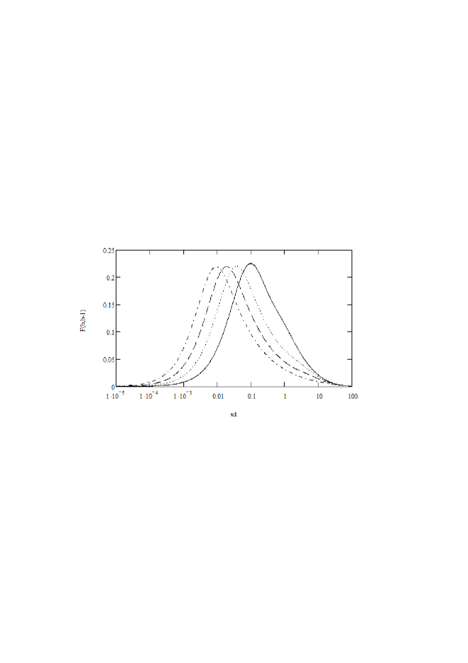
Figure 1: Full thin line we see the fidelity decay , $F(b,t)$, for $b=1$, dotted line $b=5$, dashed line $b=10$, dash dotted line $b=15$, the x axis corresponds to $\kappa t$ in a log scale.

In figure (2) we have the fidelity of the state $|b><b|(t)$ and $|b>$ for b=1, 5, 10 and 15. This is the probability of observing the state $|b>$ as function of time supposing we have prepared this state. As we can observe in this figure, the higher energy gets, the faster fidelity approaches zero (b). This means that we have a short time to measure the state before it becomes a complete statistical mixture.

Figure 2: Full thin line we see the fidelity of the state $|b><b|(t)$ and $|b>$ for $b=1$, dotted line $b=5$, dashed line $b=10$, dash dotted line $b=15$, the x axis corresponds to $\kappa t$ in a log scale.

If we consider a mixed state as (43) the $y(n)$ function has to be adapted. For the quartic oscilator que can assume that

$$\left\langle\tau\right\rangle\approx\frac{2\pi\hbar\left\langle\widehat{N}\right\rangle}{\left\langle\hat{H}_{0}\right\rangle},$$

where $\widehat{N}=\hat{a}^{\dagger}\hat{a}.$ Thus, for an initial fock state $\left|b\right\rangle,$ we have

$$\left\langle\widehat{N}_{b}(b)\right\rangle=\sum_{l=0}^{\infty}\sum_{p=0}^{b}\frac{b!(p+l)!(p+l)}{\left(p!\right)^{2}!l!(b-p)!}\times\gamma^{b+l-p}(0,t)\zeta^{2p+1}(0,t)$$ (48)

and

$$\left\langle\hat{H}_{0}(b)\right\rangle=\sum_{l=0}^{\infty}\sum_{p=0}^{b}\frac{b!(p+l)!\hbar\omega(p+l)+\lambda\hbar^{2}(p+l)^{2}}{\left(p!\right)^{2}!l!(b-p)!}\times\gamma^{b+l-p}(0,t)\zeta^{2p+1}(0,t).$$ (49)

Then we have $\left\langle\Delta E_{n}\right\rangle=\left(\left\langle\hat{H}_{0}(b)\right\rangle-\left\langle\hat{H}_{0}(b-1)\right\rangle\right)/2$ and $\left\langle\Delta\tau_{b}\right\rangle=\left(\left\langle\tau_{b}\right\rangle-\left\langle\tau_{b-1}\right\rangle\right)/2,$ and finally , for an intial state $\left|b\right\rangle$ we obtain

$$\left\langle y(b)\right\rangle=\left\langle\Delta E_{b}\right\rangle\left\langle\Delta\tau_{b}\right\rangle.$$ (50)

In figure (3) we have $\left\langle y(b)\right\rangle$ of the state $|b><b|(t)$ for b=2, 5, 10 and 15 and $\omega/\hbar\lambda=0.10$. In figure (4) we have $\left\langle y(b)\right\rangle$ of the state $|b><b|(t)$ for b=2, 5, 10 and 15 and $\omega/\hbar\lambda=10$. As we can see, the action of the environment reduces the chance of observing the spectra discreteness even for hight non linearity. The the ”lifetime” of discreteness is approximately $1/\kappa$ , thus we connected the classical limit of a spectra with the action of an environment and experimental resolution.

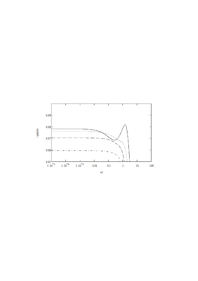
Figure 3: Full thin line we see $\left\langle y(b)\right\rangle$ of state $|b><b|(t)$ for $b=2$, dotted line $b=5$, dashed line $b=10$, dash dotted line $b=15$, the x axis corresponds to $\kappa t$ in a log scale, $\omega/\hbar\lambda=0.10$.

Figure 4: Full thin line we see $\left\langle y(b)\right\rangle$ of state $|b><b|(t)$ for $b=2$, dotted line $b=5$, dashed line $b=10$, dash dotted line $b=15$, the x axis corresponds to $\kappa t$ in a log scale, $\omega/\hbar\lambda=10$.

V Conclusion

In this work we have shown that the discrete nature of the energy levels can be accessed by classical measurements in some cases. We also defined a precise limit for this procedure using the function $y(n)=\left|\Delta E_{n}\Delta\tau_{n}\right|$ and comparing it with the time-energy uncertainty principle. This maneuver gives us a complementarity principle and a well defined mathematical limit dictated by the experiment. Of course, the fact that we are not able to recognize the discrete nature of a spectrum does not necessarily mean it is not discrete. It only means how “myope” we are, suggesting that Classical Mechanics can be viewed as a blurring of essential aspects of Quantum Mechanics and also explains why it took so long to find quantum effects. Also, as observed by many works Caldeira ; Zur1996 ; Zur2003 ; Oliveira06 ; renato2006 ; Faria07 ; Wiebe ; renato2007 a quantum system is never isolated, thus we are forced to include environment action that, in the present case, turns impractical any classical energy measurement as defined in section III, what means that otherwise we show how to get the classical limit in terms of discrete nature of the spectra.

VI References

References

- (1) Bohr, N. , Causality and Complementarity, supplementary papers edited by Jan Faye and Henry Folse as The Philosophical Writings of Niels Bohr, Vol. IV, Woodbridge: Ox Bow Press.(1998).
- (2) Bohr, N. (1920), ”On the series spectra of the elements”, Lecture before the German Physical Society in Berlin (27 April 1920), translated by A. D. Udden, in Bohr (1976), 241-282.
- (3) D. Home, Conceptual Foundations of Quantum Physics. An Overview from Modern Perspectives (Plenum Press, New York and London, 1997).
- (4) F. Laloë, Am. J. Phys. 69, 655, (2001).
- (5) W. H. Zurek and J. P. Paz, arXiv: quant-ph/9612037 v1 (1996).
- (6) Rubin, P.L. Theoretical and Mathematical Physics110, 360 (1997).
- (7) Tores Jr., M. S. and Figueiredo, J. M. A. Physica A329, 68 (2003).
- (8) De Luca, J. Phys. Rev. E71, 056210 (2005).
- (9) A. C. Oliveira and G. S. Amarante-Segundo, Phys. A, v. 388, p. 1413-1418, (2009).
- (10) Y. Yu et al., Science 296, 889 (2002).
- (11) K. Inomata et al., Phys.Rev. Lett. 95, 107005 (2005).
- (12) A. C. Oliveira and M. C. Nemes and K. M. Fonseca Romero, Phys Rev. E 68, 036214 (2003).
- (13) A. C. Oliveira and J. G. Peixoto de Faria and M. C. Nemes, Phys Rev. E 73, 046207 (2006).
- (14) J. G. Peixoto de Faria, Eur. Phys. J. D 58, 153 (2007).
- (15) L. E. Ballentine and S. M. McRac, Phys. Rev. A 58, 1799 (1998).
- (16) L. E. Ballentine, Phys. Rev. A 63, 31 (2001).
- (17) G. P. Berman et al., Phys. Rev. A 69, 062110 (2004).
- (18) N. Wiebe and L. E. Ballentine, Phys. Rev. A 72, 022109 (2005).
- (19) A. C. Oliveira, and A.R. Bosco de Magalhães, Phys. Rev. E 80 (2009) 026204.
- (20) G. B. Lemos* and F. Toscano, Phys. Rev. E 84 (2011) 016220.
- (21) A. C. Oliveira, and A.R. Bosco de Magalhães, and J. G. Peixoto Faria, Physica A, 391, 5082 (2012).
- (22) R. M. Angelo, Phys. Rev. A. 76, 052111 (2007).
- (23) L. Davidovich, M. Orzag, and N. Zagury, Phys. Rev. A 57, 2544 (1998).
- (24) L. G. Lutterbach and L. Davivovich, Phys. Rev. Lett 78, 2547 (1997).
- (25) L. G. Lutterbach and L. Davivovich, Optics Express 3, 147 (1998).
- (26) K. Banaszek, C. Radzewicz, and K. Wódkiewicz, arXiv: quant-ph/9903027 (1999).
- (27) Mukamel et al., arXiv: quant-ph/0302126 (2003).
- (28) A. Kenfact and K. Zyczkowski, arXiv:quant-ph/0406015 (2004).
- (29) F. Toscano et al., Phys. Rev. A 73, 023803 (2006).
- (30) C. W. Gardiner and P. Zoller, Quantum Noise (Springer-Verlag, Berlin, Heidelberg, 2010).
- (31) S. G. Rajeev, A theory of errors in quantum measurement, 2003, arXiv: quant-ph/0306037 (2003).
- (32) AsherPeres, Quantum Theory: Concepts and Methods (Kluver Academic Publishers, New York, Boston, Dordrecht, London, Moscow, 2002), chapter 12, item 12-8 and references therein cited.
- (33) O. Darrigol, From c-Numbers to q-Numbers The Classical Analogy in the History of Quantum Theory, University of California Press, Berkeley · Los Angeles · Oxford (1993).
- (34) A. C. Oliveira, Jour. Mod. Phys., 3, 694 (2012).
- (35) A. C. Oliveira, and M. C. Nemes, Physica Scripta 64, 279 (2001).
- (36) M. V. Berry and N. L. Balazs, J. Phys. A 12 (1978) 625.
- (37) H. J. Stöckmann, Quantum Chaos: an introduction, Cambridge University Press, New York, (2000).
- (38) D. A. Wisniacki and E. Vergini and R. M. Benito and F. Borondo, Phys. Rev. Lett. 97 (2006) 094101.
- (39) M. Novaes, and M. A. M. Aguiar, Phys. Rev. A 71 (2005) 012104.
- (40) C. Cohen-Tannouji, B. Diu, and F. Laloë, Quantum Mechanics, vol. 1 (Wiley, New York, 1977).
- (41) R. M. Eisberg, and R. Resnick, Física Quântica: Átomos, Moléculas, Sólidos, Núcleos e Partículas (Campus, São Paulo, 1994).
- (42) Richard F. Voss and Richard A. Webb Phys. Rev. Lett. 47, 265 (1981).
- (43) V. B. Braginsky, and F. Y. Khalili, Quantum Measurement (Cambridge University Press, Cambridge, 1992).
- (44) A. Isar, arXiv: quant-ph/041189 (2004).
- (45) M. Greiner et al. Nature 419, 51 (2002).
- (46) Agarwal, G. S. and Puri, R. R. Phys.Rev. A. 39, 2969 (1989).
- (47) R. M. Angelo and E. S. Cardoso and K. Furuya, Phys.Rev. A. 73, 062107 (2006).
- (48) A. O. Caldeira and A. J. Leggett Physica A 121, 587(1983). Annals of Phys. 149, 374 (1983).
- (49) W. H. Zurek Rev. Mod. Phys 75, 715 (2003).
- (50) D. M. Appleby, International Journal of Theoretical Physics,37, 1491(1998).