Abstract

In this article, we calculate the $B_{c}^{*}\to B_{c}$ electromagnetic form-factor with the three-point QCD sum rules, then study the radiative decays $B_{c}^{*\pm}\to B_{c}^{\pm}\gamma$. Experimentally, we can study the radiative transitions using the decay cascades $B_{c}^{*\pm}\to B_{c}^{\pm}\gamma\to J/\psi\ell^{\pm}\bar{\nu}_{\ell}\gamma\to\mu^{+}\mu^{-}\ell^{\pm}\bar{\nu}_{\ell}\gamma$ in the future at the LHCb.

PACS number: 13.20.Gd

Key words: $B_{c}^{*}$-meson, Radiative decays

1 Introduction

The ground state bottom-charm mesons, which lie below the $BD$, $BD^{*}$, $B^{*}D$, $B^{*}D^{*}$ thresholds, cannot annihilate into gluons due to their flavor composing, and decay weakly through $\bar{b}\to\bar{c}W^{+}$, $c\to sW^{+}$, $c\bar{b}\to W^{+}$ or decay radiatively through $b\to b\gamma$, $c\to c\gamma$ at the quark level. The pseudoscalar mesons $B_{c}^{\pm}$ decay weakly and have measurable lifetime, while the radiative transitions $B_{c}^{*\pm}\to B_{c}^{\pm}\gamma$ saturate the widths of the vector mesons $B_{c}^{*\pm}$. Experimentally, the semileptonic decays $B_{c}^{\pm}\to J/\psi\ell^{\pm}\bar{\nu}_{\ell}$, $B_{c}^{+}\to J/\psi e^{+}\bar{\nu}_{e}$ were used to measure the $B_{c}$ lifetime and the hadronic decays $B_{c}^{\pm}\to J/\psi\pi^{\pm}$ were used to measure the $B_{c}$ mass [1]. The $B_{c}^{*\pm}$ mesons have not been observed yet, but they are expected to be observed at the large hadron collider (LHC) through the radiative transitions. In the article, we calculate the $B_{c}^{*}\to B_{c}$ electromagnetic form-factor with the three-point QCD sum rules, and study the radiative decays $B_{c}^{*\pm}\to B_{c}^{\pm}\gamma$.

The QCD sum rules is a powerful nonperturbative approach in studying the heavy quarkonium states, and has given many successful descriptions of the masses, decay constants, form-factors, strong coupling constants [2, 3, 4]. The weak form-factors $B_{c}\to J/\psi$, $\eta_{c}$, $\chi_{c0}$, $\chi_{c1}$, $h_{c}$, $B$, $B_{s}$, $D$, $D_{s}$ , $B^{*}$, $B^{*}_{s}$, $D^{*}$, $D^{*}_{s}$, $D_{s1}$, etc, have been studied extensively with the three-point QCD sum rules [5, 6, 7, 8, 9], and the corresponding semileptonic decay widths have also been studied. In previous work, we calculate the $B_{c}^{*}\to\eta_{c}$ form-factors with the three-point QCD sum rules, and study the semileptonic decays $B_{c}^{*}\to\eta_{c}\ell\bar{\nu}_{\ell}$ [10]. The tiny decay widths are consistent with the expectation that the radiative transitions $B_{c}^{*\pm}\to B_{c}^{\pm}\gamma$ have the dominant branching fractions. In the past years, the radiative transitions $B_{c}^{*\pm}\to B_{c}^{\pm}\gamma$ have been studied by the (non-) relativistic potential models [11, 12, 13, 14, 15]. It is interesting to make prediction based on the nonperturbative method of QCD.

The article is arranged as follows: we study the $B_{c}^{*}\to B_{c}$ electromagnetic form-factor using the three-point QCD sum rules in Sect.2; in Sect.3, we present the numerical results and discussions; and Sect.4 is reserved for our conclusions.

2 The $B_{c}^{*}\to B_{c}$ electromagnetic form-factor with QCD sum rules

We study the $B_{c}^{*}\to B_{c}$ electromagnetic form-factor with the three-point correlation function $\Pi_{\mu\nu}(p_{1},p_{2})$,

$$\Pi_{\mu\nu}(p_{1},p_{2}) = i^{2}\int d^{4}xd^{4}ye^{ip_{2}\cdot x-ip_{1}\cdot y}\langle 0|T\{J_{5}(x)j_{\mu}(0)J_{\nu}^{\dagger}(y)\}|0\rangle\,,$$ (1)

where

$$j_{\mu}(0) = e_{b}\bar{b}(0)\gamma_{\mu}b(0)+e_{c}\bar{c}(0)\gamma_{\mu}c(0)\,,$$

$$J_{5}(x) = \bar{c}(x)i\gamma_{5}b(x)\,,$$

$$J_{\nu}(y) = \bar{c}(y)\gamma_{\nu}b(y)\,,$$ (2)

the $j_{\mu}(0)$ is the electromagnetic current, the electric charges $e_{b}=-\frac{1}{3}$ and $e_{c}=\frac{2}{3}$, the currents $J_{5}(x)$ and $J_{\nu}(y)$ interpolate the pseudoscalar and vector $B_{c}$ mesons, respectively.

We can insert a complete set of intermediate hadronic states with the same quantum numbers as the current operators $J_{5}(x)$ and $J^{\dagger}_{\nu}(y)$ into the correlation function $\Pi_{\mu\nu}(p_{1},p_{2})$ to obtain the hadronic representation [2, 3]. After isolating the ground state contributions come from the heavy mesons $B_{c}^{*}$ and $B_{c}$ , we get the following result,

$$\Pi_{\mu\nu}(p_{1},p_{2}) = \frac{\langle 0|J_{5}(0)|B_{c}(p_{2})\rangle\langle B_{c}(p_{2})|j_{\mu}(0)|B_{c}^{*}(p_{1})\rangle\langle B_{c}^{*}(p_{1})|J^{\dagger}_{\nu}(0)|0\rangle}{(M_{B_{c}}^{2}-p_{2}^{2})(M_{B_{c}^{*}}^{2}-p_{1}^{2})}+\cdots\,,$$ (3)

$$= -\frac{f_{B_{c}}M_{B_{c}}^{2}f_{B_{c}^{*}}M_{B_{c}^{*}}V(q^{2})}{(m_{b}+m_{c})(M_{B_{c}^{*}}+M_{B_{c}})(M_{B_{c}^{*}}^{2}-p_{1}^{2})(M_{B_{c}}^{2}-p_{2}^{2})}\epsilon_{\mu\nu\alpha\beta}p_{1}^{\alpha}p_{2}^{\beta}+\cdots\,,$$

where we have used the following definitions for the $B_{c}^{*}\to B_{c}$ electromagnetic form-factor and weak decay constants of the vector meson $B_{c}^{*}$ and pseudoscalar meson $B_{c}$,

$$\langle B_{c}(p_{2})|j_{\mu}(0)|B_{c}^{*}(p_{1})\rangle = \epsilon_{\mu\nu\alpha\beta}\varepsilon^{\nu}p_{1}^{\alpha}p_{2}^{\beta}\frac{V(q^{2})}{M_{B_{c}^{*}}+M_{B_{c}}}\,,$$ (4)

$$\langle 0|J_{\mu}(0)|B_{c}^{*}(p_{1})\rangle = f_{B_{c}^{*}}M_{B_{c}^{*}}\varepsilon_{\mu}\,,$$

$$\langle 0|J_{5}(0)|B_{c}(p_{2})\rangle = \frac{f_{B_{c}}M_{B_{c}}^{2}}{m_{b}+m_{c}}\,,$$ (5)

$q_{\mu}=(p_{1}-p_{2})_{\mu}$, the $\varepsilon_{\mu}$ is the polarization vector of the $B_{c}^{*}$ meson.

Now, we briefly outline the operator product expansion for the correlation function $\Pi_{\mu\nu}(p_{1},p_{2})$. We contract the quark fields in the correlation function $\Pi_{\mu\nu}(p_{1},p_{2})$ with Wick theorem firstly,

$$\Pi_{\mu\nu}(p_{1},p_{2}) = \int d^{4}xd^{4}ye^{ip_{2}\cdot x-ip_{1}\cdot y}\left\{e_{b}{\rm Tr}\left[i\gamma_{5}B^{mn}(x)\gamma_{\mu}B^{nk}(-y)\gamma_{\nu}C^{km}(y-x)\right]\right.$$ (6)

$$\left.+e_{c}{\rm Tr}\left[i\gamma_{5}B^{mn}(x-y)\gamma_{\nu}C^{nk}(y)\gamma_{\mu}C^{km}(-x)\right]\right\}\,,$$

replace the $c$ and $b$ quark propagators $C^{ij}(x)$ and $B^{ij}(x)$ with the corresponding full propagators $S_{ij}(x)$,

$$S_{ij}(x) = \frac{i}{(2\pi)^{4}}\int d^{4}ke^{-ik\cdot x}\left\{\frac{\delta_{ij}}{\!\not\!{k}-m_{Q}}-\frac{g_{s}G^{n}_{\alpha\beta}t^{n}_{ij}}{4}\frac{\sigma^{\alpha\beta}(\!\not\!{k}+m_{Q})+(\!\not\!{k}+m_{Q})\sigma^{\alpha\beta}}{(k^{2}-m_{Q}^{2})^{2}}+\frac{\delta_{ij}\langle g^{2}_{s}GG\rangle}{12}\right.$$ (7)

$$\left.\frac{m_{Q}k^{2}+m_{Q}^{2}\!\not\!{k}}{(k^{2}-m_{Q}^{2})^{4}}+\cdots\right\}\,,$$

where $Q=c,b$, $t^{n}=\frac{\lambda^{n}}{2}$, the $\lambda^{n}$ are the Gell-Mann matrixes, the $i$, $j$ are color indexes, and the $\langle g^{2}_{s}GG\rangle$ is the gluon condensate [3], then carry out the integrals. In this article, we take into account the leading-order perturbative contribution $\Pi_{\mu\nu}^{0}(p_{1},p_{2})$ and gluon condensate contribution $\Pi_{\mu\nu}^{GG}(p_{1},p_{2})$ in the operator product expansion.

The leading-order perturbative contribution $\Pi_{\mu\nu}^{0}(p_{1},p_{2})$ can be written as

$$\Pi_{\mu\nu}^{0}(p_{1},p_{2}) = \frac{3e_{b}}{(2\pi)^{4}}\int d^{4}k\frac{{\rm Tr}\left\{\gamma_{5}\left[\!\not\!{k}+\!\not\!{p}_{2}+m_{b}\right]\gamma_{\mu}\left[\!\not\!{k}+\!\not\!{p}_{1}+m_{b}\right]\gamma_{\nu}\left[\!\not\!{k}+m_{c}\right]\right\}}{\left[(k+p_{2})^{2}-m_{b}^{2}\right]\left[(k+p_{1})^{2}-m_{b}^{2}\right]\left[k^{2}-m_{c}^{2}\right]}\,,$$ (8)

$$+\frac{3e_{c}}{(2\pi)^{4}}\int d^{4}k\frac{{\rm Tr}\left\{\gamma_{5}\left[\!\not\!{k}+m_{b}\right]\gamma_{\nu}\left[\!\not\!{k}-\!\not\!{p}_{1}+m_{c}\right]\gamma_{\mu}\left[\!\not\!{k}-\!\not\!{p}_{2}+m_{c}\right]\right\}}{\left[k^{2}-m_{b}^{2}\right]\left[(k-p_{1})^{2}-m_{c}^{2}\right]\left[(k-p_{2})^{2}-m_{c}^{2}\right]}\,,$$

$$= \int ds_{1}ds_{2}\frac{\rho_{\mu\nu}(s_{1},s_{2},q^{2})}{(s_{1}-p_{1}^{2})(s_{2}-p_{2}^{2})}\,.$$

We put all the quark lines on mass-shell using the Cutkosky’s rule, and obtain the leading-order perturbative spectral density $\rho_{\mu\nu}(s_{1},s_{2},q^{2})$,

$$\rho_{\mu\nu}(s_{1},s_{2},q^{2}) = -\frac{3ie_{b}}{(2\pi)^{3}}\int d^{4}k\delta\left[(k+p_{2})^{2}-m_{b}^{2}\right]\delta\left[(k+p_{1})^{2}-m_{b}^{2}\right]\delta\left[k^{2}-m_{c}^{2}\right]$$ (9)

$${\rm Tr}\left\{\gamma_{5}\left[\!\not\!{k}+\!\not\!{p}_{2}+m_{b}\right]\gamma_{\mu}\left[\!\not\!{k}+\!\not\!{p}_{1}+m_{b}\right]\gamma_{\nu}\left[\!\not\!{k}+m_{c}\right]\right\}$$

$$-\frac{3ie_{c}}{(2\pi)^{3}}\int d^{4}k\delta\left[(k-p_{2})^{2}-m_{c}^{2}\right]\delta\left[(k-p_{1})^{2}-m_{c}^{2}\right]\delta\left[k^{2}-m_{b}^{2}\right]$$

$${\rm Tr}\left\{\gamma_{5}\left[\!\not\!{k}+m_{b}\right]\gamma_{\nu}\left[\!\not\!{k}-\!\not\!{p}_{1}+m_{c}\right]\gamma_{\mu}\left[\!\not\!{k}-\!\not\!{p}_{2}+m_{c}\right]\right\}$$

$$= -\frac{3e_{b}\epsilon_{\mu\nu\alpha\beta}p_{1}^{\alpha}p_{2}^{\beta}}{4\pi^{2}\sqrt{\lambda(s_{1},s_{2},q^{2})}}\left\{m_{b}+\frac{(m_{b}-m_{c})(s_{1}+s_{2}-q^{2}+2m_{b}^{2}-2m_{c}^{2})q^{2}}{\lambda(s_{1},s_{2},q^{2})}\right\}$$

$$-\frac{3e_{c}\epsilon_{\mu\nu\alpha\beta}p_{1}^{\alpha}p_{2}^{\beta}}{4\pi^{2}\sqrt{\lambda(s_{1},s_{2},q^{2})}}\left\{m_{c}+\frac{(m_{c}-m_{b})(s_{1}+s_{2}-q^{2}+2m_{c}^{2}-2m_{b}^{2})q^{2}}{\lambda(s_{1},s_{2},q^{2})}\right\}\,,$$

$\lambda(a,b,c)=a^{2}+b^{2}+c^{2}-2ab-2bc-2ca$, where we have used the formulae presented in Refs.[10, 16] to carry out the integrals.

We calculate the gluon condensate contribution directly and obtain the following expression,

$$\Pi_{\mu\nu}^{GG}(p_{1},p_{2}) = \frac{ie_{b}\epsilon_{\mu\nu\alpha\beta}}{4\pi^{2}}\langle\frac{\alpha_{s}GG}{\pi}\rangle\left\{-m_{b}^{2}m_{c}\left(\overline{I}_{141}+\overline{I}_{411}\right)p_{1}^{\alpha}p_{2}^{\beta}\right.$$ (10)

$$+m_{b}^{2}(m_{c}-m_{b})\left(\overline{I}^{\alpha}_{141}+\overline{I}^{\alpha}_{411}\right)q^{\beta}-m_{c}^{3}\overline{I}_{114}p_{1}^{\alpha}p_{2}^{\beta}+m_{c}^{2}(m_{c}-m_{b})\overline{I}^{\alpha}_{114}q^{\beta}$$

$$\left.-m_{b}\overline{I}^{\alpha}_{131}p_{1}^{\beta}+m_{b}\overline{I}^{\alpha}_{311}p_{2}^{\beta}-m_{c}\overline{I}_{113}p_{1}^{\alpha}p_{2}^{\beta}+m_{c}\overline{I}_{113}^{\alpha}q^{\beta}\right\}$$

$$+\frac{ie_{b}\epsilon_{\mu\nu\alpha\beta}}{24\pi^{2}}\langle\frac{\alpha_{s}GG}{\pi}\rangle\left\{(m_{b}-m_{c})\left(\overline{I}_{221}^{\alpha}+\overline{I}_{212}^{\alpha}\right)q^{\beta}+m_{c}\left(\overline{I}_{221}+\overline{I}_{212}\right)p_{1}^{\alpha}p_{2}^{\beta}\right.$$

$$\left.-2m_{b}\overline{I}_{122}^{\alpha}p_{2}^{\beta}-3(m_{b}-m_{c})\overline{I}_{122}^{\alpha}q^{\beta}-3m_{c}\overline{I}_{122}p_{1}^{\alpha}p_{2}^{\beta}\right\}$$

$$+\frac{ie_{c}\epsilon_{\mu\nu\alpha\beta}}{4\pi^{2}}\langle\frac{\alpha_{s}GG}{\pi}\rangle\left\{-m_{c}^{2}m_{b}\left(\overline{J}_{141}+\overline{J}_{411}\right)p_{1}^{\alpha}p_{2}^{\beta}\right.$$

$$+m_{c}^{2}(m_{b}-m_{c})\left(\overline{J}^{\alpha}_{141}+\overline{J}^{\alpha}_{411}\right)q^{\beta}-m_{b}^{3}\overline{J}_{114}p_{1}^{\alpha}p_{2}^{\beta}+m_{b}^{2}(m_{b}-m_{c})\overline{J}^{\alpha}_{114}q^{\beta}$$

$$\left.-m_{c}\overline{J}^{\alpha}_{131}p_{1}^{\beta}+m_{c}\overline{J}^{\alpha}_{311}p_{2}^{\beta}-m_{b}\overline{J}_{113}p_{1}^{\alpha}p_{2}^{\beta}+m_{b}\overline{J}_{113}^{\alpha}q^{\beta}\right\}$$

$$+\frac{ie_{c}\epsilon_{\mu\nu\alpha\beta}}{24\pi^{2}}\langle\frac{\alpha_{s}GG}{\pi}\rangle\left\{(m_{c}-m_{b})\left(\overline{J}_{221}^{\alpha}+\overline{J}_{212}^{\alpha}\right)q^{\beta}+m_{b}\left(\overline{J}_{221}+\overline{J}_{212}\right)p_{1}^{\alpha}p_{2}^{\beta}\right.$$

$$\left.-2m_{c}\overline{J}_{122}^{\alpha}p_{2}^{\beta}-3(m_{c}-m_{b})\overline{J}_{122}^{\alpha}q^{\beta}-3m_{b}\overline{J}_{122}p_{1}^{\alpha}p_{2}^{\beta}\right\}\,,$$

where

$$\overline{I}_{ijn} = \int d^{4}k\frac{1}{\left[(k+p_{1})^{2}-m_{b}^{2}\right]^{i}\left[(k+p_{2})^{2}-m_{b}^{2}\right]^{j}\left[k^{2}-m_{c}^{2}\right]^{n}}\,,$$

$$\overline{I}_{ijn}^{\alpha} = \int d^{4}k\frac{k^{\alpha}}{\left[(k+p_{1})^{2}-m_{b}^{2}\right]^{i}\left[(k+p_{2})^{2}-m_{b}^{2}\right]^{j}\left[k^{2}-m_{c}^{2}\right]^{n}}\,,$$

$$\overline{J}_{ijn} = \int d^{4}k\frac{1}{\left[(k+p_{1})^{2}-m_{c}^{2}\right]^{i}\left[(k+p_{2})^{2}-m_{c}^{2}\right]^{j}\left[k^{2}-m_{b}^{2}\right]^{n}}\,,$$

$$\overline{J}_{ijn}^{\alpha} = \int d^{4}k\frac{k^{\alpha}}{\left[(k+p_{1})^{2}-m_{c}^{2}\right]^{i}\left[(k+p_{2})^{2}-m_{c}^{2}\right]^{j}\left[k^{2}-m_{b}^{2}\right]^{n}}\,.$$ (11)

We take quark-hadron duality below the threshold $s^{0}_{1}$ and $s_{2}^{0}$ in the channels $B_{c}^{*}$ and $B_{c}$, respectively, perform double Borel transform with respect to the variables $P_{1}^{2}=-p_{1}^{2}$ and $P_{2}^{2}=-p_{2}^{2}$, respectively, and obtain the QCD sum rule for the electromagnetic form-factor $V(q^{2})$,

$$V(q^{2}) = \frac{(M_{B_{c}^{*}}+M_{B_{c}})(m_{b}+m_{c})}{f_{B_{c}^{*}}f_{B_{c}}M_{B_{c}^{*}}M_{B_{c}}^{2}}\exp\left(\frac{M_{B_{c}^{*}}^{2}}{M_{1}^{2}}+\frac{M_{B_{c}}^{2}}{M_{2}^{2}}\right)$$ (12)

$$\left\{\frac{3e_{b}}{4\pi^{2}}\int_{(m_{b}+m_{c})^{2}}^{s_{1}^{0}}ds_{1}\int_{(m_{b}+m_{c})^{2}}^{s_{2}^{0}}ds_{2}\frac{\mathcal{C}}{\sqrt{\lambda(s_{1},s_{2},q^{2})}}\exp\left(-\frac{s_{1}}{M_{1}^{2}}-\frac{s_{2}}{M_{2}^{2}}\right)\right.$$

$$\left[m_{b}+\frac{(m_{b}-m_{c})(s_{1}+s_{2}-q^{2}+2m_{b}^{2}-2m_{c}^{2})q^{2}}{\lambda(s_{1},s_{2},q^{2})}\right]|_{|b(s_{1},s_{2},q^{2})|\leq 1}$$

$$+\frac{3e_{c}}{4\pi^{2}}\int_{(m_{b}+m_{c})^{2}}^{s_{1}^{0}}ds_{1}\int_{(m_{b}+m_{c})^{2}}^{s_{2}^{0}}ds_{2}\frac{\mathcal{C}}{\sqrt{\lambda(s_{1},s_{2},q^{2})}}\exp\left(-\frac{s_{1}}{M_{1}^{2}}-\frac{s_{2}}{M_{2}^{2}}\right)$$

$$\left.\left[m_{c}+\frac{(m_{c}-m_{b})(s_{1}+s_{2}-q^{2}+2m_{c}^{2}-2m_{b}^{2})q^{2}}{\lambda(s_{1},s_{2},q^{2})}\right]|_{|c(s_{1},s_{2},q^{2})|\leq 1}\right\}\$$

$$-\frac{(M_{B_{c}^{*}}+M_{B_{c}})(m_{b}+m_{c})M_{1}^{2}M_{2}^{2}}{f_{B_{c}^{*}}f_{B_{c}}M_{B_{c}^{*}}M_{B_{c}}^{2}}\langle\frac{\alpha_{s}GG}{\pi}\rangle\exp\left(\frac{M_{B_{c}^{*}}^{2}}{M_{1}^{2}}+\frac{M_{B_{c}}^{2}}{M_{2}^{2}}\right)$$

$$\left\{\frac{e_{b}m_{b}^{2}}{4\pi^{2}}\left[m_{c}\left(I_{0}^{141}+I_{0}^{411}\right)+(m_{c}-m_{b})\left(I_{10}^{141}+I_{01}^{141}+I_{10}^{411}+I_{01}^{411}\right)\right]\right.$$

$$+\frac{e_{b}m_{c}^{2}}{4\pi^{2}}\left[m_{c}I_{0}^{114}+(m_{c}-m_{b})\left(I_{10}^{114}+I_{01}^{114}\right)\right]-\frac{e_{b}m_{b}}{4\pi^{2}}\left(I_{01}^{131}+I_{10}^{311}\right)$$

$$+\frac{e_{b}m_{c}}{4\pi^{2}}\left(I_{0}^{113}+I_{10}^{113}+I_{01}^{113}\right)+\frac{e_{b}(m_{b}-m_{c})}{24\pi^{2}}\left(I_{10}^{221}+I_{01}^{221}+I_{10}^{212}+I_{01}^{212}\right)$$

$$+\frac{e_{b}m_{b}}{12\pi^{2}}I_{10}^{122}-\frac{e_{b}(m_{b}-m_{c})}{8\pi^{2}}\left(I_{10}^{122}+I_{01}^{122}\right)-\frac{e_{b}m_{c}}{24\pi^{2}}\left(I_{0}^{221}+I_{0}^{212}-3I_{0}^{122}\right)$$

$$+\frac{e_{c}m_{c}^{2}}{4\pi^{2}}\left[m_{b}\left(J_{0}^{141}+J_{0}^{411}\right)+(m_{b}-m_{c})\left(J_{10}^{141}+J_{01}^{141}+J_{10}^{411}+J_{01}^{411}\right)\right]$$

$$+\frac{e_{c}m_{b}^{2}}{4\pi^{2}}\left[m_{b}J_{0}^{114}+(m_{b}-m_{c})\left(J_{10}^{114}+J_{01}^{114}\right)\right]-\frac{e_{c}m_{c}}{4\pi^{2}}\left(J_{01}^{131}+J_{10}^{311}\right)$$

$$+\frac{e_{c}m_{b}}{4\pi^{2}}\left(J_{0}^{113}+J_{10}^{113}+J_{01}^{113}\right)+\frac{e_{c}(m_{c}-m_{b})}{24\pi^{2}}\left(J_{10}^{221}+J_{01}^{221}+J_{10}^{212}+J_{01}^{212}\right)$$

$$\left.+\frac{e_{c}m_{c}}{12\pi^{2}}J_{10}^{122}-\frac{e_{c}(m_{c}-m_{b})}{8\pi^{2}}\left(J_{10}^{122}+J_{01}^{122}\right)-\frac{e_{c}m_{b}}{24\pi^{2}}\left(J_{0}^{221}+J_{0}^{212}-3J_{0}^{122}\right)\right\}\,,$$

$$= e_{b}V_{1}(q^{2})+e_{c}V_{2}(q^{2})\,,$$ (13)

where

$$b(c_{1},c_{2},q^{2}) = \frac{2s_{1}(s_{2}+m_{c}^{2}-m_{b}^{2})-(s_{1}+s_{2}-q^{2})(s_{1}+m_{c}^{2}-m_{b}^{2})}{\sqrt{\lambda(s_{1},s_{2},q^{2})\lambda(s_{1},m_{c}^{2},m_{b}^{2})}}\,,$$

$$c(c_{1},c_{2},q^{2}) = \frac{2s_{1}(s_{2}+m_{b}^{2}-m_{c}^{2})-(s_{1}+s_{2}-q^{2})(s_{1}+m_{b}^{2}-m_{c}^{2})}{\sqrt{\lambda(s_{1},s_{2},q^{2})\lambda(s_{1},m_{c}^{2},m_{b}^{2})}}\,,$$

$${\mathcal{C}} = \sqrt{\frac{4\pi\alpha_{s}^{\mathcal{C}}}{3v_{1}}\left[1-\exp\left(-\frac{4\pi\alpha_{s}^{\mathcal{C}}}{3v_{1}}\right)\right]^{-1}}\sqrt{\frac{4\pi\alpha_{s}^{\mathcal{C}}}{3v_{2}}\left[1-\exp\left(-\frac{4\pi\alpha_{s}^{\mathcal{C}}}{3v_{2}}\right)\right]^{-1}}\,,$$

$$v_{1} = \sqrt{1-\frac{4m_{b}m_{c}}{s_{1}-(m_{b}-m_{c})^{2}}}\,,$$

$$v_{2} = \sqrt{1-\frac{4m_{b}m_{c}}{s_{2}-(m_{b}-m_{c})^{2}}}\,,$$

the explicit expressions of the $I_{0}^{ijn}$, $I_{10}^{ijn}$, $I_{01}^{ijn}$, $J_{0}^{ijn}$, $J_{10}^{ijn}$, $J_{01}^{ijn}$ are presented in the appendix. For the heavy quarkonium states $B_{c}^{*}$ and $B_{c}$, the relative velocities of quark movement are small, we should account for the Coulomb-like $\frac{\alpha_{s}^{\mathcal{C}}}{v}$ corrections. After taking into account all the Coulomb-like contributions shown in Fig.1, we obtain the coefficient $\mathcal{C}$ to dress the quark-meson vertex [7, 8].

At the recoil momentum close to zero, the heavy quark velocities are small below the thresholds $s_{1}^{0}$ and $s_{2}^{0}$, the ladder Feynman diagrams shown in Fig.1 are calculated in the nonrelativistic approximation, and result in the coefficient $\mathcal{C}$ to dress the quark-meson vertex. In our previous work on the two-point QCD sum rules for the $B_{c}^{*}$ mesons [17], we observed that the perturbative ${\mathcal{O}}(\alpha_{s})$ corrections to the leading-order spectral density $\rho_{0}(s)$ can be approximated by $\rho_{0}(s)\frac{2\pi\alpha_{s}^{\mathcal{C}}}{3v}$ with the assumption ${\alpha_{s}^{\mathcal{C}}}=\alpha_{s}(\mu)$, and accounted for all the Coulomb-like contributions (or all the perturbative corrections approximately) by multiplying the $\rho_{0}(s)$ with the coefficient $\mathcal{C}$,

$${\mathcal{C}} = \frac{4\pi\alpha_{s}^{\mathcal{C}}}{3v}\frac{1}{1-\exp\left(-\frac{4\pi\alpha_{s}^{\mathcal{C}}}{3v}\right)}=1+\frac{2\pi\alpha_{s}^{\mathcal{C}}}{3v}+\frac{1}{12}\left(\frac{4\pi\alpha_{s}^{\mathcal{C}}}{3v}\right)^{2}-\frac{1}{720}\left(\frac{4\pi\alpha_{s}^{\mathcal{C}}}{3v}\right)^{4}+\cdots\,.$$ (15)

In the case of the three-point QCD sum rules, the perturbative ${\mathcal{O}}(\alpha_{s})$ corrections to the leading order spectral densities are available only for the electromagnetic form-factors of the $\pi$ and $\rho$ mesons [18], we expect to approximate the perturbative ${\mathcal{O}}(\alpha_{s})$ corrections by multiplying the leading order spectral densities with $\frac{\pi\alpha_{s}^{\mathcal{C}}}{3v_{1}}+\frac{\pi\alpha_{s}^{\mathcal{C}}}{3v_{2}}$, and take into account all the Coulomb-like interactions (or all the perturbative corrections approximately) by multiplying the leading order spectral densities with the coefficient $\mathcal{C}$ [7, 8]. Direct but formidable calculations of the perturbative corrections are still needed to validate or invalidate the present approximation. In the region of physical resonances, the most essential effect comes from the normalization factor $\mathcal{C}$. In the case of the two-point sum rules, the normalization factor $\mathcal{C}$ leads to a double-triple multiplication of the tree-level value of the spectral densities numerically [19]. The coefficient $\mathcal{C}$ survives beyond the zero recoil limit, or at least serve as upper bounds on the form-factors in the QCD sum rules [7, 8]. In this article, we take the approximation ${\alpha_{s}^{\mathcal{C}}}=\alpha_{s}(\mu)$ in numerical calculation as in our previous work [17].

Figure 1: The ladder Feynman diagrams for the Coulomb-like interactions.

In the physical region $q^{2}=0$, the constraints $|b(c_{1},c_{2},0)|\leq 1$ and $|c(c_{1},c_{2},0)|\leq 1$ lead to the inequations,

$$-1\leq\frac{s_{1}+(m_{b}^{2}-m_{c}^{2})}{\sqrt{\lambda(s_{1},m_{1}^{2},m_{2}^{2})}}\leq 1\,,$$

$$-1\leq\frac{s_{1}+(m_{c}^{2}-m_{b}^{2})}{\sqrt{\lambda(s_{1},m_{1}^{2},m_{2}^{2})}}\leq 1\,,$$ (16)

those constraints cannot be satisfied. In this article, we calculate the electromagnetic form-factors $V_{1}(q^{2})$ and $V_{2}(q^{2})$ at the space-like region $Q^{2}=-q^{2}=(1.0-5.4)\,\rm{GeV}^{2}$, then fit the electromagnetic form-factors with suitable analytical functions, and obtain the value $V(0)$ by analytically continuing the variable $q^{2}$ to the physical region.

3 Numerical results and discussions

The pseudoscalar mesons $B_{c}$ have been studied by the full QCD sum rules [5, 6, 20, 21] and the potential approach combined with the QCD sum rules [11, 22], while the vector mesons $B_{c}^{*}$ have been studied by the full QCD sum rules [6, 17, 21]. The predictions for the masses and decay constants are $f_{B_{c}}=(0.383\pm 0.027)\,\rm{GeV}$ [5]; $f_{B_{c}^{*}}\approx f_{B_{c}}=(360\pm 60)\,\rm{MeV}$, $M_{B_{c}}\approx 6.35\,\rm{GeV}$ [6]; $f_{B_{c}}=(460\pm 60)\,\rm{MeV}$ [11]; $f_{B_{c}^{*}}=(0.384\pm 0.032)\,\rm{GeV}$, $M_{B_{c}^{*}}=(6.337\pm 0.052)\,\rm{GeV}$ [17]; $f_{B_{c}}=(300\pm 65)\,\rm{MeV}$, $M_{B_{c}}=(6.25\pm 0.20)\,\rm{GeV}$ [20]; $f_{B_{c}}=(566\pm 28)\,\rm{MeV}$, $f_{B_{c}^{*}}\approx(0.346\pm 0.025)\,\rm{GeV}$, $M_{B_{c}}\approx(6.969\pm 0.18)\,\rm{GeV}$, $M_{B_{c}^{*}}\approx(6.855\pm 0.18)\,\rm{GeV}$ [21]. The predictions for the mass $M_{B_{c}}$ are consistent with (or much larger than) the average value $M_{B_{c}}=(6.277\pm 0.006)\,\rm{GeV}$ listed in the Review of Particle Physics [23], while the predictions for the decay constant $f_{B_{c}}$ vary in large ranges.

The values of the decay constants from other theoretical calculations also vary in large ranges, $f_{B^{*}_{c}}=f_{B_{c}}=500\,\rm{MeV}$, $512\,\rm{MeV}$, $479\,\rm{MeV}$ and $687\,\rm{MeV}$ from the Buchmuller-Tye potential, power-law potential, logarithmic potential and Cornell potential, respectively [12]; $f_{B_{c}^{*}}=f_{B_{c}}=517\,\rm{MeV}$ from the Richardson s potential [13]; $f_{B_{c}}=433\,\rm{MeV}$ and $f_{B_{c}^{*}}=503\,\rm{MeV}$ from the relativistic quark model with an special potential [14]; $f_{B_{c}}=(410\pm 40)\,\rm{MeV}$ from the relativized quark (Godfrey-Isgur) model [15]; $f_{B_{c}}=(420\pm 13)\,\rm{MeV}$ from the lattice non-relativistic QCD [24]; $f_{B_{c}}=(395\pm 15)\,\rm{MeV}$ from the QCD-motivated potential model [25]; $f_{B_{c}^{*}}=f_{B_{c}}=315^{+26}_{-50}\,\rm{MeV}$ from the shifted $N$-expansion method [26]; $f_{B_{c}}=377\,\rm{MeV}$ ($360\,\rm{MeV}$, $440\,\rm{MeV}$), $f_{B_{c}^{*}}=398\,\rm{MeV}$ ($387\,\rm{MeV}$, $440\,\rm{MeV}$) from the light-front quark model [27]([28],[29]); $f_{B_{c}^{*}}=(453\pm 20)\,\rm{MeV}$, $f_{B_{c}}=(438\pm 10)\,\rm{MeV}$ from the field correlator method [30]; $f_{B_{c}}=(322\pm 42)\,\rm{MeV}$, $f_{B_{c}^{*}}=(418\pm 24)\,\rm{MeV}$ from the Bethe-Salpeter equation [31].

Although the values of the decay constants vary in large ranges, some theoretical calculations indicate that the decay constants have the relation $f_{B_{c}^{*}}\approx({\rm or=})f_{B_{c}}$ [6, 12, 13, 26, 27, 28, 29, 30]. In the early work [32], Gershtein and Khlopov obtained a simple relation $f_{ij}\propto m_{i}+m_{j}$ for the decay constant $f_{ij}$ of the pseudoscalar meson having the constituent quarks $i$ and $j$, such simple relation does not work well enough for both the light and heavy quarks. In this article, we choose the values $f_{B_{c}^{*}}=0.384\,\rm{GeV}$, $M_{B_{c}^{*}}=6.337\,\rm{GeV}$ from the recent analysis based on the QCD sum rules [17], $f_{B_{c}}=395\rm{MeV}$ from the QCD-motivated potential model [25], $M_{B_{c}}=6.277\,\rm{GeV}$ from the Particle Data Group [23]. The decay constants have the relation $f_{B_{c}^{*}}\approx f_{B_{c}}$, the masses have the splitting $M_{B_{c}^{*}}-M_{B_{c}}=60\,\rm{MeV}$. The uncertainties of the electromagnetic form-factor $V(q^{2})$ originate from the decay constants can be estimated as $\frac{\delta f_{B_{c}^{*}}}{f_{B_{c}^{*}}}+\frac{\delta f_{B_{c}}}{f_{B_{c}}}$. The calculations based on the nonrelativistic renormalization group indicate that $M_{B_{c}(1^{-})}-M_{B_{c}(0^{-})}=(50\pm 17{}^{+15}_{-12})\,\rm{MeV}$ [33], the mass $M_{B_{c}^{*}}=6.337\,\rm{GeV}$ from the QCD sum rules is satisfactory. Accordingly, we take the threshold parameters and Borel parameters as $s_{1}^{0}=s_{2}^{0}=(45\pm 1)\,\rm{GeV}^{2}$, $M_{1}^{2}=M_{2}^{2}=(5-7)\,\rm{GeV}^{2}$ from the QCD sum rules [17].

The value of the gluon condensate $\langle\frac{\alpha_{s}GG}{\pi}\rangle$ has been updated from time to time, and changes greatly, we use the recently updated value $\langle\frac{\alpha_{s}GG}{\pi}\rangle=(0.022\pm 0.004)\,\rm{GeV}^{4}$ [34]. For the heavy quark masses, we take the $\overline{MS}$ masses $m_{c}(m_{c}^{2})=(1.275\pm 0.025)\,\rm{GeV}$ and $m_{b}(m_{b}^{2})=(4.18\pm 0.03)\,\rm{GeV}$ from the Particle Data Group [23], and take into account the energy-scale dependence of the $\overline{MS}$ masses from the renormalization group equation,

$$m_{c}(\mu^{2}) = m_{c}(m_{c}^{2})\left[\frac{\alpha_{s}(\mu)}{\alpha_{s}(m_{c})}\right]^{\frac{12}{25}}\,,$$

$$m_{b}(\mu^{2}) = m_{b}(m_{b}^{2})\left[\frac{\alpha_{s}(\mu)}{\alpha_{s}(m_{b})}\right]^{\frac{12}{23}}\,,$$

$$\alpha_{s}(\mu) = \frac{1}{b_{0}t}\left[1-\frac{b_{1}}{b_{0}^{2}}\frac{\log t}{t}+\frac{b_{1}^{2}(\log^{2}{t}-\log{t}-1)+b_{0}b_{2}}{b_{0}^{4}t^{2}}\right]\,,$$ (17)

where $t=\log\frac{\mu^{2}}{\Lambda^{2}}$, $b_{0}=\frac{33-2n_{f}}{12\pi}$, $b_{1}=\frac{153-19n_{f}}{24\pi^{2}}$, $b_{2}=\frac{2857-\frac{5033}{9}n_{f}+\frac{325}{27}n_{f}^{2}}{128\pi^{3}}$, $\Lambda=213\,\rm{MeV}$, $296\,\rm{MeV}$ and $339\,\rm{MeV}$ for the flavors $n_{f}=5$, $4$ and $3$, respectively [23]. In this article, we take the typical energy scale $\mu=2\,\rm{GeV}$ as in Ref.[17].

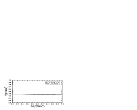
Figure 2: The electromagnetic form-factors $V_{1}(q^{2}=-1\,\rm{GeV}^{2})$ and $V_{2}(q^{2}=-1\,\rm{GeV}^{2})$ with variations of the Borel parameters $M_{1}^{2}$ and $M_{2}^{2}$.

In Fig.2, we plot the electromagnetic form-factors at $q^{2}=-Q^{2}=-1\,\rm{GeV}^{2}$ with variations of the Borel parameters $M_{1}^{2}$ and $M_{2}^{2}$. From the figure, we can see that the values are rather stable with variations of the Borel parameters. In calculations, we observe that $0.0001\leq\exp(-\frac{s_{1}^{0}}{M_{1}^{2}})\leq 0.00186$ and $0.0001\leq\exp(-\frac{s_{2}^{0}}{M_{2}^{2}})\leq 0.00186$, the contributions from high resonances and continuum states are greatly suppressed, furthermore, the contributions from the gluon condensate are of minor importance, the operator product expansion is well convergent.

We take into account all the uncertainties come from the input parameters, such as the heavy quark masses, threshold parameters, Borel parameters, $\dots$, obtain numerical values of the electromagnetic form-factors $V_{1}(Q^{2})$, $V_{2}(Q^{2})$ and $V(Q^{2})$ from Eqs.(12-13), and show them explicitly in Figs.3-4. We express the electromagnetic form-factors in the standard form $f(Q^{2})=\overline{f}(Q^{2})\pm\delta f(Q^{2})$ numerically, where the $f(Q^{2})$ denotes the electromagnetic form-factors $V_{1}(Q^{2})$, $V_{2}(Q^{2})$, $V(Q^{2})$, the $\overline{f}(Q^{2})$ denotes the central values, and the $\delta f(Q^{2})$ denotes the uncertainties, then fit the numerical values of the $V_{1}(Q^{2})$, $V_{2}(Q^{2})$ at $Q^{2}=(1-5.4)\,\rm{GeV}^{2}$ and $V(Q^{2})$ at $Q^{2}=(1-4.2)\,\rm{GeV}^{2}$ into the following analytical functions,

$$V_{1}(Q^{2}) = \frac{A}{1+BQ^{2}}\,,$$

$$V_{2}(Q^{2}) = \frac{C}{1+DQ^{2}+EQ^{4}}\exp\left(-FQ^{2}\right)\,,$$ (18)

$$V(Q^{2}) = G\exp\left(-HQ^{2}\right)+T\,,$$ (19)

with the $\bf\rm MINUIT$, and determine the parameters,

$$A = 2.8905\pm 0.45717\,,$$

$$B = 0.056340\pm 0.056316\,\rm{GeV}^{-2}\,,$$

$$C = 10.978\pm 10.369\,,$$

$$D = 0.20611\pm 0.94270\,\rm{GeV}^{-2}\,,$$

$$E = 0.017546\pm 0.55116\,\rm{GeV}^{-4}\,,$$

$$F = 0.44543\pm 1.4035\,\rm{GeV}^{-2}\,,$$

$$G = 7.0807\pm 1.8756\,,$$

$$H = 0.67821\pm 0.22875\,\rm{GeV}^{-2}\,,$$

$$T = -0.66869\pm 0.35949\,.$$ (20)

From Figs.3-4, we can see that the fitted functions can reproduce the central values of the form-factors at large ranges $Q^{2}=(1-10)\,\rm{GeV}^{2}$, and the fitted functions $V_{1}(Q^{2})$, $V_{2}(Q^{2})$ and $V(Q^{2})$ work well.

We continue the $Q^{2}$ to the physical region $Q^{2}=0$ analytically to obtain the physical electromagnetic form-factor $V(0)$,

$$V(0) = 6.35517\pm 6.91435\,\,\,{\rm from\,\,\,Eq.(18)}\,,$$ (21)

$$= 6.41201\pm 1.90974\,\,\,{\rm from\,\,\,Eq.(19)}\,.$$

The curve of the fitted function $V_{2}(Q^{2})$ is very steep, the value $V_{2}(0)=10.978\pm 10.369$ has too large uncertainty, the resulting uncertainty of the $V(0)$ is also too large, we discard the value $V(0)=6.35517\pm 6.91435$. On the other hand, the value $V(0)=6.41201\pm 1.90974$ from Eq.(19) has much smaller uncertainty, i.e. less than $30\%$. We take the value $V(0)=6.41201\pm 1.90974$, and obtain the radiative decay width,

$$\Gamma(B_{c}^{*}\to B_{c}\gamma) = \frac{\alpha|V(0)|^{2}\left(M_{B_{c}^{*}}+M_{B_{c}}\right)\left(M_{B_{c}^{*}}-M_{B_{c}}\right)^{3}}{24M_{B_{c}^{*}}^{3}}$$ (22)

$$= 133.9^{+91.6}_{-67.9}\,\rm{eV}\,\left(133.9\pm 79.7\,\rm{eV}\right)\,,$$

where the fine constant $\alpha=\frac{1}{137}$, the asymmetric uncertainty comes from the formula $V^{2}(0)-\overline{V}^{2}(0)$, while the symmetric uncertainty in the bracket comes from the approximation $V^{2}(0)-\overline{V}^{2}(0)\approx\pm 2\overline{V}(0)\delta V(0)$ with $V(0)=\overline{V}(0)\pm\delta V(0)$. From Eq.(22) we can see that the decay width is sensitive to the mass splitting $M_{B_{c}^{*}}-M_{B_{c}}$ as $\Gamma(B_{c}^{*}\to B_{c}\gamma)\propto(M_{B_{c}^{*}}-M_{B_{c}})^{3}$. The present prediction $\Gamma(B_{c}^{*}\to B_{c}\gamma)=133.9^{+91.6}_{-67.9}\,\rm{eV}\,\left(133.9\pm 79.7\,\rm{eV}\right)$ is compatible with previous values $60\,\rm{eV}$ from the nonrelativistic potential [11], $134.5\,\rm{eV}$ from non-relativistic potential model [12], $59\,\rm{eV}$ from Richardson s potential [13], $33\,\rm{eV}$ from the relativistic quark model with an special potential [14], $80\,\rm{eV}$ from the relativized quark (Godfrey-Isgur) model [15]. In Ref.[10], we have used a larger decay constant $f_{B_{c}^{*}}=0.79\,\rm{GeV}$ rather than $0.384\,\rm{GeV}$, the smaller decay constant $f_{B_{c}^{*}}=0.384\,\rm{GeV}$ leads to the semileptonic decay widths $\Gamma(B_{c}^{*}\to\eta_{c}\ell\bar{\nu}_{\ell})\sim 10^{-5}\,\rm{eV}$. The branching fractions of the semileptonic decays $B_{c}^{*}\to\eta_{c}\ell\bar{\nu}_{\ell}$ are of the order $10^{-7}\sim 10^{-6}$, which supports that the dominant decay model is $B_{c}^{*}\to B_{c}\gamma$. We can search for the $B_{c}^{*}$ mesons using the decay cascades $B_{c}^{*\pm}\to B_{c}^{\pm}\gamma\to J/\psi\ell^{\pm}\bar{\nu}_{\ell}\gamma\to\mu^{+}\mu^{-}\ell^{\pm}\bar{\nu}_{\ell}\gamma$.

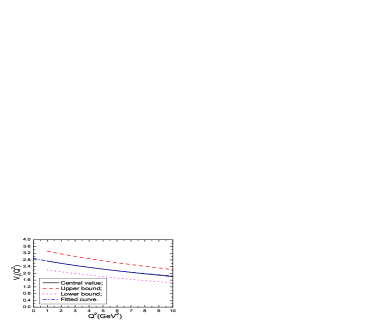
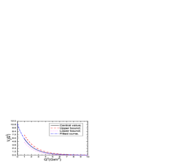
Figure 3: The electromagnetic form-factors $V_{1}(Q^{2})$ and $V_{2}(Q^{2})$, where the ”Fitted curve” denotes the central values of the fitted functions.

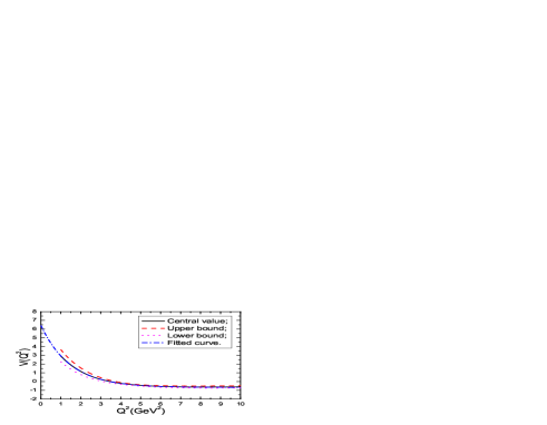
Figure 4: The electromagnetic form-factor $V(Q^{2})$, where the ”Fitted curve” denotes the central value of the fitted function.

4 Conclusion

In this article, we calculate the $B_{c}^{*}\to B_{c}$ electromagnetic form-factor with the three-point QCD sum rules, and obtain the numerical values for the form-factor at momentum transfer $Q^{2}=-q^{2}=(1.0-5.4)\,\rm{GeV}^{2}$, then fit the form-factors to analytical functions to obtain the physical value, and study the radiative decays $B_{c}^{*\pm}\to B_{c}^{\pm}\gamma$. We expect to study the radiative transitions using the decay cascades $B_{c}^{*\pm}\to B_{c}^{\pm}\gamma\to J/\psi\ell^{\pm}\bar{\nu}_{\ell}\gamma\to\mu^{+}\mu^{-}\ell^{\pm}\bar{\nu}_{\ell}\gamma$ in the future at the LHCb.

Appendix

The explicit expressions of the $I_{0}^{ijn}$, $I_{10}^{ijn}$, $I_{01}^{ijn}$, $J_{0}^{ijn}$, $J_{10}^{ijn}$, $J_{01}^{ijn}$,

$$iI_{0}^{ijn} = B_{-p_{1}^{2}\rightarrow M_{1}^{2}}B_{-p_{2}^{2}\rightarrow M_{2}^{2}}\overline{I}_{ijn}$$ (23)

$$= B_{P_{1}^{2}\rightarrow M_{1}^{2}}B_{P_{2}^{2}\rightarrow M_{2}^{2}}\frac{(-1)^{i+j+n}i}{\Gamma(i)\Gamma(j)\Gamma(n)}\int d^{4}K\int_{0}^{\infty}d\alpha d\beta d\gamma\alpha^{i-1}\beta^{j-1}\gamma^{n-1}$$

$$\exp\left\{-\alpha(K+P_{1})^{2}-\beta(K+P_{2})^{2}-\gamma K^{2}-\alpha m_{b}^{2}-\beta m_{b}^{2}-\gamma m_{c}^{2}\right\}$$

$$= \frac{(-1)^{i+j+n}i\pi^{2}}{\Gamma(i)\Gamma(j)\Gamma(n)(M_{1}^{2})^{i}(M_{2}^{2})^{j}(M^{2})^{n-2}}\int_{0}^{1}d\lambda\frac{\lambda^{1-i-j}}{(1-\lambda)^{n-1}}$$

$$\exp\left\{-\frac{(1-\lambda)Q^{2}}{\lambda(M_{1}^{2}+M_{2}^{2})}-\frac{m_{b}^{2}}{\lambda M^{2}}-\frac{m_{c}^{2}}{(1-\lambda)M^{2}}\right\}$$

$$= \frac{(-1)^{i+j+n}i\pi^{2}}{\Gamma(i)\Gamma(j)\Gamma(n)(M_{1}^{2})^{i}(M_{2}^{2})^{j}(M^{2})^{n-2}}\int_{0}^{\infty}d\tau(\tau+1)^{i+j+n-4}\tau^{1-i-j}$$

$$\exp\left\{-\frac{1}{\tau}\left(\frac{Q^{2}}{M_{1}^{2}+M_{2}^{2}}+\frac{m_{b}^{2}}{M^{2}}\right)-\frac{m_{b}^{2}+m_{c}^{2}}{M^{2}}-\tau\frac{m_{c}^{2}}{M^{2}}\right\}\,,$$

$$iI^{\mu}_{ijn} = B_{-p_{1}^{2}\rightarrow M_{1}^{2}}B_{-p_{2}^{2}\rightarrow M_{2}^{2}}\overline{I}^{\mu}_{ijn}$$ (24)

$$= \frac{(-1)^{i+j+n+1}i\pi^{2}}{\Gamma(i)\Gamma(j)\Gamma(n)(M_{1}^{2})^{i+1}(M_{2}^{2})^{j}(M^{2})^{n-3}}\int_{0}^{\infty}d\tau(\tau+1)^{i+j+n-3}\tau^{1-i-j}$$

$$\exp\left\{-\frac{1}{\tau}\left(\frac{Q^{2}}{M_{1}^{2}+M_{2}^{2}}+\frac{m_{b}^{2}}{M^{2}}\right)-\frac{m_{b}^{2}+m_{c}^{2}}{M^{2}}-\tau\frac{m_{c}^{2}}{M^{2}}\right\}p_{1}^{\mu}$$

$$+\frac{(-1)^{i+j+n+1}i\pi^{2}}{\Gamma(i)\Gamma(j)\Gamma(n)(M_{1}^{2})^{i}(M_{2}^{2})^{j+1}(M^{2})^{n-3}}\int_{0}^{\infty}d\tau(\tau+1)^{i+j+n-3}\tau^{1-i-j}$$

$$\exp\left\{-\frac{1}{\tau}\left(\frac{Q^{2}}{M_{1}^{2}+M_{2}^{2}}+\frac{m_{b}^{2}}{M^{2}}\right)-\frac{m_{b}^{2}+m_{c}^{2}}{M^{2}}-\tau\frac{m_{c}^{2}}{M^{2}}\right\}p_{2}^{\mu}$$

$$= iI_{10}^{ijn}p_{1}^{\mu}+iI_{01}^{ijn}p_{2}^{\mu}\,,$$

$$J_{0}^{ijn} = I_{0}^{ijn}|_{m_{b}\leftrightarrow m_{c}}\,,$$

$$J_{10}^{ijn} = I_{10}^{ijn}|_{m_{b}\leftrightarrow m_{c}}\,,$$

$$J_{01}^{ijn} = I_{01}^{ijn}|_{m_{b}\leftrightarrow m_{c}}\,,$$

$$M^{2} = \frac{M_{1}^{2}M_{2}^{2}}{M_{1}^{2}+M_{2}^{2}}\,,$$ (25)

where we have used the Borel transform $B_{P^{2}\rightarrow M^{2}}\exp(-\alpha P^{2})=\delta(1-\alpha M^{2})$. Those analytical expressions are slightly different from that obtained in Ref.[7], they are both correct.

References

[1] A. Abulencia et al, Phys. Rev. Lett. 97 (2006) 012002;
V. Abazov et al, Phys. Rev. Lett. 102 (2009) 092001;
T. Aaltonen et al, Phys. Rev. Lett. 100 (2008) 182002;
V. M. Abazov et al, Phys. Rev. Lett. 101 (2008) 012001.
[2] M. A. Shifman, A. I. Vainshtein and V. I. Zakharov, Nucl. Phys. B147 (1979) 385, 448.
[3] L. J. Reinders, H. Rubinstein and S. Yazaki, Phys. Rept. 127 (1985) 1.
[4] P. Colangelo and A. Khodjamirian, arXiv:hep-ph/0010175.
[5] E. Bagan, H. G. Dosch, P. Gosdzinsky, S. Narison and J. M. Richard, Z. Phys. C64 (1994) 57.
[6] P. Colangelo, G. Nardulli and N. Paver, Z. Phys. C57 (1993) 43.
[7] V. V. Kiselev, A. K. Likhoded and A. I. Onishchenko, Nucl. Phys. B569 (2000) 473.
[8] V. V. Kiselev, Int. J. Mod. Phys. A11 (1996) 3689;
V. V. Kiselev, A. E. Kovalsky and A. K. Likhoded, Nucl. Phys. B585 (2000) 353.
[9]
T. M. Aliev and M. Savci, Eur. Phys. J. C47 (2006) 413;
N. Ghahramany, R. Khosravi and K. Azizi, Phys. Rev. D78 (2008) 116009;
K. Azizi, R. Khosravi and V. Bashiry, Eur. Phys. J. C56 (2008) 357;
K. Azizi, F. Falahati, V. Bashiry and S. M. Zebarjad, Phys. Rev. D77 (2008) 114024;
K. Azizi and R. Khosravi, Phys. Rev. D78 (2008) 036005;
N. Ghahramany, R. Khosravi and K. Azizi, Phys. Rev. D78 (2008) 116009;
K. Azizi, H. Sundu and M. Bayar, Phys. Rev. D79 (2009) 116001.
[10] Z. G. Wang, arXiv:1209.1157.
[11] S. S. Gershtein, V. V. Kiselev, A. K. Likhoded and A. V. Tkabladze, Phys. Rev. D51 (1995) 3613;
S. S. Gershtein, V. V. Kiselev, A. K. Likhoded and A. V. Tkabladze, Phys. Usp. 38 (1995) 1.
[12] E. J. Eichten and C. Quigg, Phys. Rev. D49 (1994) 5845.
[13] L. P. Fulcher, Phys. Rev. D60 (1999) 074006.
[14] D. Ebert, R. N. Faustov and V. O. Galkin, Phys. Rev. D67 (2003) 014027.
[15] S. Godfrey, Phys. Rev. D70 (2004) 054017.
[16] B .L. Ioffe and A. V. Smilga, Nucl. Phys. B216 (1983) 373;
D. S. Du, J. W. Li and M. Z. Yang, Eur. Phys. J. C37 (2004) 173.
[17] Z. G. Wang, arXiv:1203.6252.
[18] V. V. Braguta and A. I. Onishchenko, Phys. Lett. B591 (2004) 267;
V. V. Braguta and A. I. Onishchenko, Phys. Rev. D70 (2004) 033001.
[19] V. A. Novikov, L. B. Okun, M. A. Shifman, A. I. Vainshtein, M. B. Voloshin and V. I. Zakharov, Phys. Rept. 41 (1978) 1.
[20] M. Chabab, Phys. Lett. B325 (1994) 205.
[21] S. Narison, Phys. Lett. B210 (1988) 238.
[22] V. V. Kiselev and A. V. Tkabladze, Phys. Rev. D48 (1993) 5208.
[23] J. Beringer et al, Phys. Rev. D86 (2012) 010001.
[24] B. D. Jones and R. M. Woloshyn, Phys. Rev. D60 (1999) 014502.
[25] V. V. Kiselev, Central Eur. J. Phys. 2 (2004) 523.
[26] S. M. Ikhdair and R. Sever, Int. J. Mod. Phys. A21 (2006) 6699.
[27] H. M. Choi and C. R. Ji, Phys. Rev. D80 (2009) 054016.
[28] C. W. Hwang, Phys. Rev. D81 (2010) 114024.
[29] R. C. Verma, J. Phys. G39 (2012) 025005.
[30] A. M. Badalian, B. L. G. Bakker and Yu. A. Simonov, Phys. Rev. D75 (2007) 116001.
[31] G. Cvetic, C. S. Kim, G. L. Wang and W. Namgung, Phys. Lett. B596 (2004) 84;
G. L. Wang, Phys. Lett. B633 (2006) 492.
[32] S. S. Gershtein, M. Yu. Khlopov, JETP Lett. 23 (1976) 338;
M. Yu. Khlopov, Sov. J. Nucl. Phys. 28 (1978) 583.
[33] A. A. Penin, A. Pineda, V. A. Smirnov and M. Steinhauser, Phys. Lett. B593 (2004) 124.
[34] S. Narison, Phys. Lett. B693 (2010) 559; S. Narison, Phys. Lett. B706 (2012) 412;
S. Narison, Phys. Lett. B707 (2012) 259.