Unusual mechanism of vortex viscosity generated by mixed normal modes in superconductors with broken time
reversal symmetry
Mihail Silaev
O. V. Lounasmaa Laboratory, P.O. Box 15100, FI-00076
Aalto University, Finland
Institute for Physics of
Microstructures RAS, 603950 Nizhny Novgorod, Russia.
Department of Theoretical Physics, The Royal
Institute of Technology, Stockholm, SE-10691 Sweden
Department of Physics, University of Massachusetts Amherst, MA
01003 USA
Egor Babaev
Department of Theoretical Physics, The Royal
Institute of Technology, Stockholm, SE-10691 Sweden
Department of Physics, University of Massachusetts Amherst, MA
01003 USA
Abstract
We show that under certain conditions multiband
superconductors with broken time-reversal symmetry have a new
vortex viscosity-generating mechanism which is different from that
in conventional superconductors. It appears due to the existence
of mixed superfluid phase-density mode inside vortex core. This
new contribution is dominant near the time reversal symmetry
breaking phase transition. The results could be relevant for three
band superconductor .
pacs:
74.25.QP, 74.25.Fy, 73.40.Gk
Recent discoveries of many novel multiband superconducting
compounds have motivated the current quest of theoretical
understanding of their basic properties. Especially strong impact
has the recent discovery of iron based superconductors
FeAs . Namely it was discussed in Ng ; StanevTesanovic
that such superconductors can break time reversal symmetry because
these system can have frustrated ground state values of the order
parameter phase differences in different bands . In that case a ground state has a
broken
time reversal symmetry (BTRS) which is associated with the complex conjugate of the order parameter
.
Therefore such superconductors break symmetry
Johan . Physically this implies existence of persistent
”Josephson current” between the three bands which is different for
two ground states. It was recently demonstrated that such physics
very likely occurs in
strongly hole doped Chubukov .
Alternatively the other scenarios of time reversal symmetry
breakdown in iron-based superconductors have been discussed
recently Other .
In this kind of BTRS state there appear new phenomena which are
absent in conventional and even extended wave multiband
superconductors. Indeed it has been shown to support a new kind of
topological defects - skyrmions Babaev ,
Leggett’s mode which becomes massless at the phase transition Lin ,
as well as mixed phase-density collective modes in state Johan . Moreover even in the frustrated
systems, time reversal symmetry breakdown can occur inside vortex
excitationsJohan . Beyond the mean field approximation and
for sufficiently strong frustration of interband interactions such
systems can have an unusual normal state
which breaks symmetry as a precursor to
a superconducting phase
transitionBabaevSudbo .
Since the system can break time reversal symmetry at certain
doping Chubukov , the superconducting state in the immediate
vicinity of the time reversal symmetry breaking phase transition
should be very interesting because of the existence of a diverging
length scale associated with the symmetry breakdown. In this
paper we show that the BTRS superconducting state with vortices
has highly unusual thermodynamic and transport properties near the
symmetry breaking transition. The peculiarities of vortex
state can be helpful to obtain experimental identification of BTRS
superconductivity in particular compounds.
We employ the three band Ginzburg-Landau (GL) expansion of the
free energy density
(1)
Here, are the order parameters in each band labelled by
band index and the second term is interband Josephson
coupling energy characterized by interband coupling constants
. The field is vector potential. For formal
microscopic justification of multiband GL functionals see
silaev , GL expansion for three band BTRS superconductor was
recently studied in detail inChubukov where it was shown
that the doping level in determines the
interband pairing interaction between electron and hole pockets
. The relation to our parameters is following
and which
is the interaction between hole pockets. Such an expansion may
contain also other terms which however will not change
quantitatively conclusions of this paper, thus we choose to work
with the minimal model.
First we investigate the equilibrium vortex structures in three
band superconductor.
We substitute the order parameters to GL equation in
the form where is real
and separate the real and imaginary parts introducing the gauge
invariant superfluid velocities
.
It should be noted that even when
a ground state has only broken symmetry, the GL model
(Unusual mechanism of vortex viscosity generated by mixed normal modes in superconductors with broken time
reversal symmetry) allows for topological excitations with
phase differences of order parameter components
Johan .
In the particular case of axially symmetric single vortex in
BTRS phase this results in the radial dependence of the order parameter phases
(we assume that vortex center is at the origin ).
Thus the additional degree of freedom due to the frustrated
phase difference in three component system allows for a
static mixed phase-density mode which appears inside
vortex cores in BTRS phase. To explore its impact on the vortex physics
we employ the minimal model which in particular describes possible BTRS
transition to the state in
Chubukov .
For such choice of GL coefficients we will use an
ansatz for vortex solutions and
. The GL equations in this case read
(2)
where and
. For the vector potential we use a radial
gauge .
First let us consider the modification of asymptotical
properties of the system (2) far from the vortex
center during the BTRS transition. At small couplings
the system is in the plain
symmetry breaking state with the relative phase between
superconducting components . The critical value
of coupling separating the and bulk phases
is given by , where
and are bulk values of the amplitudes
and . Beyond the threshold
the time reversal symmetry is broken
so that . This behavior of bulk
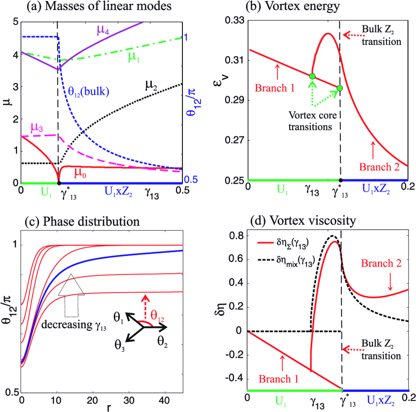
is shown in Fig.(1)a by blue dashed curve.
In phase when the mode shown by
red solid line is a pure phase one which is decoupled from order
parameter densities. However in general it can still be excited
inside vortex core due to nonlinearities. In this case
symmetry can be broken locally in the core but not in the bulk
Johan . At the critical point of symmetry breakdown in
the bulk of the system the mixed mode has zero mass
remm2 .
At critical point, existence of massless mode results in a
power-law localization of vortex-core solutions. Note that in this
case the anharmonism in Eq.(2) is important.
Here at large the field deviations from bulk values can be
found in the form of power law expansions (the details of
asymptotic analysis are given in Supplementary material)
.
Now let us search numerically for vortex solutions of Eqs.
(2) to show that the vortex energy and viscosity
have anomalies at phase transition. As will be discussed
below, it is important to take into account the following three
circumstances for the accurate description of this anomalous
behavior at the BTRS phase transition (i) phase-density modes
mixing, (ii) appearance of massless mode and (iii)anharmonism in Eqs.(2).
To find possible vortex structures we implement a numerical solution of the full GL system
(2) supplemented by the Ampere’s law for magnetic field.
To define the boundary conditions for the fields we consider a vortex lattice and thus use the
circular cell approximation (see also remark remark ). At
the boundary of the Weigner-Seits cell the fields satisfy
and .
The former determines the order parameter to be periodic function
and the latter one provides magnetic
flux quantization. Also from the first
of Eqs.(2), it follows that the boundary condition for
the phase is .
We investigated the vortex structure as function of interband
coupling which is determined by the doping level in
compoundChubukov .
We have found that the relative phases of the order parameter
components in BTRS superconductor
always have non-trivial variation
in contrast to the usual
time-reversal invariant case. Examples of phase distributions are
shown in Fig.(1)c for a set of values
decreasing towards the vortex core transition point
which will be discussed below. We will see that
such phase variation produces an additional friction force on the
moving vortices.
For the vortex solution is unique. Its
energy is shown in Fig.(1)b by solid red curve
denoted as Branch 2. Even at the point of bulk transition
the energy remains finite due to the discussed above anharmonism of the massless
mixed mode in Eqs.(2). However its contribution provides a peak of vortex energy close to
(where this mode becomes massless).
On the other hand time reversal invariant state at
can support two different vortex
structures. To demonstrate it we note at first that the
Eqs.(2) always have solution with the relative phase
. We find that this solution is stable in
domain. At the same range of parameters the symmetry can be
broken in the vortex core leading to the non-trivial variation of
with asymptotic boundary condition
. We find numerically that
these vortex structures can coexist at a certain region
(note that one of the solutions can be
unstable remm in the coexistence region, but this does not
affect conclusions of this paper). The corresponding branches of
vortex energy are shown in Fig.(1b). There is a
critical value of interband coupling
where the two branches merge. This critical coupling is determined
as the eigenvalue of linearized first equation in the system
(2) which we write in the form of Sturm-Liouville
equation
where and
is a hermitian operator.
This means (see Supplementary Material) that at the amplitude of relative phase
variation is given by so that the energy difference
between Branch 1 and Branch 2 is linear
.
Figure 1:
(a) Masses of the asymptotic mixed modes of the system
(2). The GL parameters are
, ,
, and .
The modes corresponds to
symmetric excitations with . The modes
break this symmetry. By dashed
blue line in (a) the ground state (bulk) phase difference is shown.
(b) Two branches of vortex energy. Branch 1 corresponds to the
vortex solutions which do not break time reversal symmetry.
Branch 2 corresponds to the solutions with non-homogeneous relative phase
(i.e. BTRS solutions). (c) Relative phase distribution
inside vortex core corresponding to the Branch 2.
For decreasing one first meets the second order phase transition in bulk where the characteristic scale
of variation
of is the largest (blue curve). At the critical value of the
Branches 1 and 2 merge when the amplitude of decreases to zero as .
(d) Vortex viscosity variation
(red solid line is total viscosity and black dashed line
is mixed mode contribution).
The obtained BTRS modification of vortex core structure is manifested transport properties determined by
vortex viscosity.
To describe a non-equilibrium process of vortex motion,
we use
time-dependent GL model (TDGL) (for a review of TDGL approach see e.g.KopninBook ; Dorsey ) generalized to a multiband case
(3)
where , are damping constants and is the potential of a quasistationary electric
field.
Choosing Couloumb gauge for the vector potential we obtain the Poisson equation (see Supplementary
material for detailed discussion)
(4)
where is a normal state electric conductivity. Equation (4)
will be employed to calculate the distribution of electric field generated by a moving vortex.
Vortex motion introduces
a distortion of the order parameter and vector potential fields.
For a slow vortex motion with a given velocity we calculate the time dependence by making
Galilean transformation of equilibrium
fields so that .
We now assume that
and search for the electrostatic potential in the form
.
The resulting equations read
(5)
(6)
where .
Note that in Eq.(6) the derivatives
can be expressed through the two functions and
using the condition for the radial current to be zero .
In the circular cell approximation the boundary condition require
the tangential component of the electric field to be zero
. Recalling that
we obtain at
and .
Also from the Eqs.(5,6) follows that
.
At first we note that Eq.(5) coincides with that
for the vortices in time reversal invariant superconductors (see
e.g. KopninBook ; Dorsey ). It determines Bardeen-Stephen
vortex viscosity BardeenStephen . The second
Eq.(6) determines qualitatively new part of the
scalar potential which appears due to the phase-density mixed mode
in BTRS superconductor. The source in the r.h.s. of this equation
is determined by the radial dependencies of the relative
phase [example is shown in the
Fig.(1)c].
Consider now electric field distribution generated by a moving
vortex. The electric field can be written as a superposition of
two terms where
and
. The first term here
is a usual dipole-like field induced around moving vortex. The
second term is the mixed mode contribution which
exists only in BTRS superconductors.
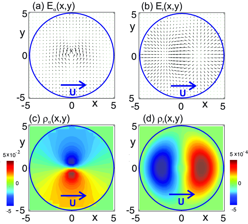
Distributions of and components
of the electric field are shown in the Fig.(2) a,b. From
Fig.(2)a one can see that the component
determines the average electric field in the sample
where is the average magnetic
induction. The other component shown in
Fig.(2) b does not contribute to the average .
The relation between vortex velocity and
transport current is in general determined by the
balance of the forces acting on the moving vortex. There are two of them: Lorentz
force from the transport current and the force from the
environment given by the expression (under the
assumption that London penetration length is much larger than the
vortex core size)
(7)
where we introduced gauge invariant scalar potential
. To find a linear response of
the environment we need to keep the
terms in Eq.(7) up to the first order in vortex
velocity. In this approximation the force from the environment provides
viscous drag which has the general form where is vortex viscosity. We find that in BTRS
superconductor it can be presented as a
superposition of three terms of different physical origin
.
Here the first two terms appear in ordinary
viscous vortex motion: these are the Tinkham TinkhamBook
and
Bardeen-Stephen BardeenStephen contributions.
The third term is completely new and appears due to
the electric mixed phase-density mode in the BTRS vortex
core:
(8)
where we put for well-separated vortices.
The physical origin of viscosity (8) is the electric field
excitation due to the mixed mode. The corresponding electric field pattern
and charge density around moving vortex is shown in Figs.(2)b,d.
Figure 2: (a,b) The distributions
of (a) dipole-like and (b) induced by mixed mode parts of the total electric field (shown by arrows)
in the unit cell around the vortex moving with velocity .
(c,d) The distribution of electric charge around the moving
vortex. (c) which coincides with the charge
in time reversal invariant superconductor. (d)
appears in BTRS superconductor.By blue solid circle the boundary of circular cell is shown.
We calculated the total vortex viscosity by solving
Eqs.(5,6) using the vortex structure
determined by static GL Eqs.(2). We find a striking
behavior of viscosity near the BTRS transition shown in
Fig.1d as function of interband coupling
. The mixed mode contribution (shown by black dashed
line) has a pronounced maximum near BTRS phase transition where
the mixed mode becomes massless. The viscosity however
still remains finite even at the
critical point due to the anharmonism in Eqs.(2)
which provides a power-law decay for the phase-density mode
contribution to viscosity as well as to the vortex energy . The
conventional Tinkham and Bardeen- Stephen contributions are
monotonic functions of . Summing up all contributions
we find that here the behavior of the total viscosity is dominated
by the mixed mode near the BTRS transition. It is shown by solid
red line which features a pronounced peak. This anomalous behavior
is realized for vortex structures belonging to Branch 2 with BTRS
either in the bulk at or in
the vortex core at . On the other hand
vortex solution without BTRS corresponding to the Branch 1 has
monotonic viscosity. Comparing Figs.1b and
1d one can see that the vortex energy and viscosity
behave rather similar as functions of .
In conclusion we reported a new mechanism contributing to vortex viscosity
in BTRS superconductors.
The results are generic for BTRS superconductors with mode mixing.
In particular it is not specific to three-band superconductor but
should also apply to BTRS states with different number of bands
or different interband frustration which exhibit mode mixing (some
of which were discussed in weston ). It leads to a
pronounced anomaly at the phase transition where time reversal
symmetry is broken.
Thus one can potentially
observe this phase transition
by measuring the anomalous behavior of both
thermodynamic properties (vortex energy determines
the lower critical field ) and
transport properties such as flux flow resistance which is
determined by vortex viscosity. It can be utilized to detect
possible state in .
We thank Daniel Weston for discussions. MS was supported by the
Swedish Research Council, Russian Foundation for Basic Research
Grants No 11-02-00891, 13-02-97126 and Russian President
scholarship (SP- 6811.2013.5), EB was supported by the US National
Science Foundation CAREER Award No. DMR-0955902, and
by Knut and Alice Wallenberg Foundation through the Royal Swedish Academy of Sciences,
Swedish Research Council.
I Supplementary material
I.1 Power law asymptotic of order parameter fields in zero mass regime
We consider the system
(9)
(10)
(11)
where and
. For the vector potential we use the
radial gauge .
We are interested in particular case when coupling parameters
satisfy the condition . In this case the mass of phase
density mixed mode is zero and the
asymptotic of coupled phase density fluctuation far from the
vortex core has power law behavior. We search the deviations of
order parameter density and phase from bulk values in the form of
power law expansion
(12)
Substituting this ansatz into the system
(9,10,11) we
require that the lowest order terms have the same dependence on
. This condition determines the exponents and
in (12). Furthermore we obtain the linear system
to determine coefficients in Eq.(12)
(13)
(14)
(15)
For the parameters employed for numerical calculations we obtain
, and .
I.2 Vortex structure near the critical point
The critical point separates regimes in region with single
and double solutions for the vortex structure. The solution with
spatial variation of relative phase continuously emerges at
where is given
by the eigenvalue of linear equation which can be written in the
form
(16)
where and
(17)
is a hermitian operator and therefore has orthogonal
eigenfunctions. This form allows to find approximate solution of
nonlinear Eq.(9) for small values of
.
We search the solution of nonlinear
Eq.(9) in the form
where is the
normalized eigenfunction of Eq.(16) and
is a small correction.
It collects the contribution of higher levels of the operator (17) and therefore is orthogonal to
so that
(18)
To determine the amplitude we rewrite Eq.(9) in the form
(19)
where the last term is nonlinear part
obtained with the help of Taylor expansion .
Taking the inner product of both parts of Eq.(19)
with and employing the hermiticity of
operator and orthogonality (18) we get
the amplitude
(20)
Thus we obtain that at the vortex
structure can have two solutions. One is that with constant
interband phase and the second one is with
the phase variation given by the eigenfunction of operator
(17) with the amplitude
given by
Eq.(20).
I.3 Time-dependent Ginzburg-Landau theory and forces acting on moving vortex in three-component superconductor
We describe the non-equilibrium process of vortex motion near the critical temperature with
time-dependent GL model generalized to a two-gap superconductor
(21)
where , is the electric potential,
are damping constants.
The expression for the supercurrent is then
where
and for the normal current where
. Note that
normal and superconducting current can convert into each other thus they are not
separately conserved. For the superfluid current we have an
expression so that
. Hence from Eq.(3) we obtain that
where . Taking into account
the total current conservation
we can get the Poisson equation for quasistationary electric field with the electric charge
density given by so that
(22)
Assuming the Coloumb gauge for the vector potential we obtain the Poisson equation
(23)
which we employ to calculate the distribution of the
scalar potential generated by the moving vortex.
Steady state vortex motion with constant velocity U is
determined by the force balance between
Lorentz force acting on the vortex from external
transport current and force from the environment .
The force acting on the moving vortices
is determined by the variation of free energy due to the
small vortex displacementKopninBook ; Dorsey . In general the variation of the free energy is
The last two terms here can be found using the identity
therefore neglecting the surface term
Besides the variation of the free energy we take into account the
interaction of vortices with transport current created by the
external source. It is given by
According to the conventional procedure we consider the
variation of the free energy due to the vortex displacement
described by
(24)
(25)
Lorentz force
Now we consider the action of the homogeneous transport
current on vortex. To calculate the force acting on
vortex we evaluate the energy change due the infinitesimal
translations of vortex center. Then the elementary work of the external force has
the form
where .
Now we use the following identities
to obtain
where is the vorticity direction.
Therefore the force is
Force from the environment
To calculate the force from the environment we should consider the energy variations due
to displacement
and .
Then we can make use of Eq.(21) which results
Further we use the fact and transform the above equation as follows
(26)
The last two terms can be written using the identity
Therefore neglecting the surface term we get
Now let us make use of the Eqs. (21) to substitute
(27)
which finally yields
For the typical type-II superconductors the last term is usually
neglected. Then we obtain the force acting on the unit length of moving vortex
line from the environment
(28)
References
(1)
Y. Kamihara, T. Watanabe, M. Hirano, and H. Hosono, J. Am. Chem.
Soc. 130, 3296 (2008).
(2)
T. K. Ng and N. Nagaosa, Europhys. Lett. 87, 17003 (2009).
(3)
V. Stanev and Z. Tesanovic, Phys. Rev. B 81, 134522 (2010).
(4) J. Carlstrom, J. Garaud, and E. Babaev, Phys. Rev. B
84, 134518 (2011).
(5)
Saurabh Maiti, Andrey V. Chubukov, Phys. Rev. B 87, 144511
(2013).
(6)
W.-C. Lee, S.-C. Zhang, and C. Wu, Physical Review Letters 102, 217002 (2009); C. Platt, R. Thomale, C. Honerkamp, S.-C.
Zhang, and W. Hanke, Phys. Rev. B 85, 180502 (2012).
(7)
J.Garaud, J.Carlstrom, and E. Babaev, Phys. Rev. Lett. 107,
197001 (2011); J. Garaud, J. Carlstrom, E. Babaev, M. Speight
Phys. Rev. B 87, 014507 (2013).
(8) S.-Z. Lin and X. Hu, Physical Review Letters 108, 177005
(2012).
(10)
M. Silaev, E. Babaev
Phys. Rev. B 85, 134514 (2012).
(11)
In the phase-only London model this divergence was identified
earlier as the massless Leggett mode in Lin .
(12)
The existence of a diverging length scale at the phase
transition and
mixing of phase difference and density
modes dictates that there should be diverging coherence length at
the TRSB phase transition while magnetic field penetration length
should stay finite. This in turns implies that if the system
should generically have “type-1.5” regime Johan in the
vicinity of TRSB state with one coherence length larger and other
smaller than the magnetic field penetration length (if the system
is not a type-I superconductor).
Here we consider the case of vortex lattice (e.g.
large fields). Results should also apply to interiour of
macroscopically large vortex clusters.
(13)
The stability analysis, requires relaxing axially symmetric
ansatz. It is beyond the scope of this paper and will be presented
elsewhere.
(14)
N. B. Kopnin, Theory of nonequlibrium superconductivity,
Oxford University Press, (2001).
(15)
A. T. Dorsey, Phys. Rev. B 46, 8376 (1992).
(16)
J. Bardeen and M.J.Stephen Phys. Rev. 140, 1197 (1965).
(17)
M. Tinkham, Introduction to superconductivity, Dover
Publications (2004).