On the tritronquée solutions of P${}_{\mbox{\rm\scriptsize I}}^{2}$

Abstract.

For equation P${}_{\mbox{\rm\tiny I}}^{2}$, the second member in the P${}_{\mbox{\rm\tiny I}}$ hierarchy, we prove existence of various degenerate solutions depending on the complex parameter $t$ and evaluate the asymptotics in the complex $x$ plane for $|x|\to\infty$ and $t=o(x^{2/3})$. Using this result, we identify the most degenerate solutions $u^{(m)}(x,t)$, $\hat{u}^{(m)}(x,t)$, $m=0,\dots,6$, called tritronquée, describe the quasi-linear Stokes phenomenon and find the large $n$ asymptotics of the coefficients in a formal expansion of these solutions. We supplement our findings by a numerical study of the tritronquée solutions.

1. Introduction

Equation P${}_{\mbox{\rm\scriptsize I}}^{2}$, the second member in the hierarchy of ODEs associated with the classical first Painlevé equation P${}_{\mbox{\rm\scriptsize I}}$, $y_{xx}=6y^{2}+x$, cf. [24], is the 4th order ODE

$$u_{xxxx}+10u_{x}^{2}+20uu_{xx}+40(u^{3}-6tu+6x)=0$$ (1.1)

depending on $t\in\mathbb{C}$ parametrically. In the last decades, this ODE has attracted significant attention [7, 9, 14, 15] justified by its various applications in mathematics and physics.

An important class of applications of P${}_{\mbox{\rm\scriptsize I}}^{2}$ concerns the description of some critical regimes in random matrix models, as well as in the asymptotics of semi-classical orthogonal polynomials and related Fredholm determinants, see e.g. [13, 12]. Furthermore a particular solution to the P${}_{\mbox{\rm\scriptsize I}}^{2}$  equation is conjectured to describe a certain class of critical regimes to solutions of Hamiltonian PDEs [36, 14, 15]. This conjecture is known as the universality conjecture for Hamiltonian PDEs. So far it has been proved only for the Korteweg-de Vries equation (KdV)

$$u_{t}+uu_{x}+\tfrac{1}{12}u_{xxx}=0,$$ (1.2)

and for its hierarchy [9, 11]. It is known that the KdV equation is compatible with the P${}_{\mbox{\rm\scriptsize I}}^{2}$ equation. Its solutions allow one to construct a 4-parameter family of so-called isomonodromic solutions to the KdV equation.

It is a remarkable fact that, from the point of view of physical applications, the most interesting solutions to the classical Painlevé equations and their higher order analogs are those with a quasi-stationary behavior. For instance, applying equation P${}_{\mbox{\rm\scriptsize I}}^{2}$ to string theory, Brezin, Marinari, Parisi [7] and Moore [33] argued that, for $t=0$, there exists a regular solution $U_{0}(x,t=0)$ to (1.1) real on the real line with the asymptotic behavior

$$U_{0}(x,t=0)\simeq\pm|6x|^{\frac{1}{3}},\quad x\rightarrow\pm\infty.$$

Dubrovin [14] conjectured the existence of the solution $U_{0}(x,t)$, which has to be pole free and regular on the real axis, for any $t\in{\mathbb{R}}$. The uniqueness of the real and regular on the real line solution to P${}_{\mbox{\rm\scriptsize I}}^{2}$ for $t=0$ was proved in [26]. The existence of such a solution was established by Claeys and Vanlessen in [13] for any $t$.

Below, we call the solution $U_{0}(x,t)$ tritronquée. This term originates from the classical paper of P. Boutroux [6] devoted to the asymptotic analysis of solutions to the P${}_{\mbox{\rm\scriptsize I}}$ equation. In particular, he has shown that, though the generic asymptotic solutions to P${}_{\mbox{\rm\scriptsize I}}$ are described using the modulated elliptic Weierstraß$\wp$-function, there exist five special directions at infinity along which the elliptic asymptotics degenerates to trigonometric ones. According to Boutroux, such trigonometric asymptotic solutions are called “tronquée”. “Bitronquée” solutions are those 1-parameter solutions whose leading order algebraic asymptotic term, $y_{as}\sim\pm\sqrt{-x/6}$, admits an analytic continuation from the special ray into one of the adjacent complex sectors. “Tritronquée” solutions are particular 0-parameter solutions admitting an analytic continuation from the ray to the interior of both the adjacent complex sectors. Remarkably, the latter asymptotic solutions remain quasi-stationary in four of a total of five complex sectors separated by the above mentioned special rays.

In the present paper, we describe a set of similar solutions to equation P${}_{\mbox{\rm\scriptsize I}}^{2}$ using extensively the Riemann-Hilbert (RH) problem approach. We prove that the physically interesting solution $U_{0}(x,t)$ real and regular on the real line solution has an extension to the complex $x$ plane with uniform algebraic asymptotics in the union of two sectors of the complex plane

$$U_{0}(x,t)\simeq-\sqrt[3]{6}\,x^{1/3},\quad x\to\infty,\\ \arg x\in\bigl{[}-\tfrac{3\pi}{7}-\tfrac{3}{7}\arctan\tfrac{1}{\sqrt{5}},\tfrac{3\pi}{7}+\tfrac{3}{7}\arctan\tfrac{1}{\sqrt{5}}\bigr{]}\cup\\ \cup\bigl{[}3\pi-\tfrac{3}{7}\arctan\tfrac{1}{\sqrt{5}},3\pi+\tfrac{3}{7}\arctan\tfrac{1}{\sqrt{5}}\bigr{]},$$ (1.3)

see Figure 1.1.

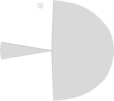
Figure 1.1. Sector for the algebraic asymptotic behavior of the solution $U_{0}(x)$ as $t=0$.

We also prove the existence and uniqueness of the solution $V_{0}(x,t)$ to P${}_{\mbox{\rm\scriptsize I}}^{2}$ with the uniform algebraic asymptotics in the sector of the $x$ complex plane

$$V_{0}(x,t)\simeq-\sqrt[3]{6}\,x^{1/3},\quad x\to\infty,\\ \arg x\in\bigl{[}3\pi-\tfrac{6\pi}{7}+\tfrac{3}{7}\arctan\tfrac{1}{\sqrt{5}},3\pi+\tfrac{6\pi}{7}-\tfrac{3}{7}\arctan\tfrac{1}{\sqrt{5}}\bigr{]},\hfill$$ (1.4)

see Figure 1.2.

Figure 1.2. Sector for the algebraic asymptotic behavior of the solution $V_{0}(x)$ as $t=0$.

Similarly to $U_{0}(x,t)$, the solution $V_{0}(x,t)$ is real on the real line but, in contrast to $U_{0}(x,t)$, it is singular on the positive part of the real line. In the interior of the overlapping complex sector containing the negative real line, the solutions $U_{0}(x,t)$ and $V_{0}(x,t)$ differ by exponentially small terms while in two other overlapping complex sectors, $U_{0}(x,t)$ and $V_{0}(x,t)$ have different leading asymptotic behavior due to different choices of the branches of the cubic root of $x$.

With the results of Shimomura [35] on the Painlevé property of P${}_{\mbox{\rm\scriptsize I}}^{2}$, the solutions $U_{0}(x,t)$ and $V_{0}(x,t)$, whose existence for large $x$ in the above sectors is proved below, extend to a globally defined meromorphic function on the complex plane. We illustrate the behavior of $U_{0}(x,t)$, $V_{0}(x,t)$ numerically. The results can be summarized in the following conjecture:

Conjecture 1.1.

The solutions $U_{0}$ and $V_{0}$ are pole free in the whole sectors of the complex plane specified in (1.3) and (1.4) respectively.

We show that $V_{0}(x,t)$ and $U_{0}(x,t)$ are the members of the families of 0-parameter solutions $\{V_{m}(x,t)\}_{m=0}^{6}$ and $\{U_{m}(x,t)\}_{m=0}^{6}$ which we call the tritronquée solutions of type I and type II, respectively. The solutions of each family can be constructed using a $7$-th order rotational symmetry applied to $V_{0}(x,t)$ and $U_{0}(x,t)$, respectively.

In the overlapping domains where the above mentioned solutions exhibit identical power series expansion, we compute the exponentially small differences between them and thus establish the so-called quasi-linear Stokes phenomenon for equation P${}_{\mbox{\rm\scriptsize I}}^{2}$.

The structure of the paper is the following. In Section 2, we describe the RH problem implied by the linear system in the auxiliary “spectral” variable whose isomonodromy deformations are controlled by P${}_{\mbox{\rm\scriptsize I}}^{2}$. Section 3 is devoted to a short description of the “spectral” curve associated with P${}_{\mbox{\rm\scriptsize I}}^{2}$ and to the model algebraic curve used to construct the asymptotic solution to P${}_{\mbox{\rm\scriptsize I}}^{2}$ of our interest. In Section 4, assuming the triviality of some of the Stokes multipliers, we prove the asymptotic solvability of the RH problem as the pair $(x,t)$ belongs to a particular domain of ${\mathbb{C}}^{2}$ and find 2-parameter families of the quasi-stationary solutions to P${}_{\mbox{\rm\scriptsize I}}^{2}$. In Section 5, we find 1- and 0-parameter intersections of the found 2-parameter families called below the bi- and tritronquée solutions and describe the quasi-linear analog of the Stokes phenomenon. Finally, in Section 6, we present a numerical study of the tritronquée solutions $V_{0}(x,t)$ and $U_{0}(x,t)$.

2. Riemann-Hilbert problem associated with equation P${}_{\mbox{\rm\scriptsize I}}^{2}$

Equation P${}_{\mbox{\rm\scriptsize I}}^{2}$ admits an isomonodromy interpretation. Namely it can be expressed as the compatibility of a linear systems for a complex $2\times 2$ matrix valued function $\Psi=\Psi(\lambda,x,t)$, cf. [26, 8],

$$\Psi_{\lambda}=A\Psi,$$ (2.1)

$$\Psi_{x}=B\Psi,$$ (2.2)

where

$$\begin{split}A=&\tfrac{1}{60}\bigl{[}-u_{x}\lambda-3uu_{x}-\tfrac{1}{4}u_{xxx}\bigr{]}\sigma_{3}+\tfrac{1}{30}\bigl{[}\lambda^{2}+u\lambda+\tfrac{3}{2}u^{2}+\tfrac{1}{4}u_{xx}-15t\bigr{]}\sigma_{+}\\ &\hskip-21.68121pt+\tfrac{1}{30}\bigl{[}\lambda^{3}-u\lambda^{2}-(\tfrac{1}{2}u^{2}+\tfrac{1}{4}u_{xx}+15t)\lambda+2u^{3}-\tfrac{1}{4}u_{x}^{2}+\tfrac{1}{2}uu_{xx}+30x\bigr{]}\sigma_{-},\end{split}$$

$$B= \begin{pmatrix}0&1\\ \lambda-2u&0\end{pmatrix}$$

and $\sigma_{3}=(\begin{smallmatrix}1&0\\ 0&-1\end{smallmatrix})$, $\sigma_{+}=(\begin{smallmatrix}0&1\\ 0&0\end{smallmatrix})$, $\sigma_{-}=(\begin{smallmatrix}0&0\\ 1&0\end{smallmatrix})$. Indeed the compatibility condition of equations (2.1) and (2.2) gives $A_{x}-B_{\lambda}+[A,B]=0$ which implies the P${}_{\mbox{\rm\scriptsize I}}^{2}$ equation (1.1), while the compatibility of (2.1) with the linear equation

$$\begin{split}\Psi_{t}&=C\Psi\\ C&=\tfrac{1}{3}\begin{pmatrix}\tfrac{1}{2}u_{x}&-\lambda-u\\ -(\lambda^{2}-u\lambda-2u^{2}-\tfrac{1}{2}u_{xx})&-\tfrac{1}{2}u_{x}\end{pmatrix}\end{split}$$ (2.3)

gives $A_{t}-C_{\lambda}+[A,C]=0$ which implies the KdV equation (1.2).

The primary object of our study is equation (2.1) with the irregular singularity at $\lambda=\infty$. The canonical solutions of (2.1) satisfying (2.2) and (2.3) are uniquely characterized by their asymptotics

$$\begin{split}\Psi_{k}(\lambda)&=\lambda^{-\frac{1}{4}\sigma_{3}}\dfrac{\sigma_{3}+\sigma_{1}}{\sqrt{2}}\left(I+\dfrac{u}{2\lambda}\sigma_{1}+\dfrac{iu_{x}}{4\lambda^{\frac{3}{2}}}\sigma_{2}+{\mathcal{O}}(\lambda^{-2})\right)e^{(\theta(\lambda)-\frac{H_{1}}{\sqrt{\lambda}}-\frac{H_{0}}{3\lambda^{3/2}})\sigma_{3}},\\ \theta(\lambda)&=\tfrac{\lambda^{\frac{7}{2}}}{105}-\tfrac{t}{3}\lambda^{\frac{3}{2}}+x\lambda^{\frac{1}{2}},\;\;\lambda\to\infty,\quad\arg\lambda\in\bigl{(}-\tfrac{3\pi}{7}+\tfrac{2\pi}{7}k,\tfrac{\pi}{7}+\tfrac{2\pi}{7}k\bigr{)},\quad k\in{\mathbb{Z}},\end{split}$$ (2.4)

where $\sigma_{1}=\sigma_{+}+\sigma_{-}$ and $i\sigma_{2}=\sigma_{+}-\sigma_{-}$. Here $H_{0}$ and $H_{1}$ are the functions of the coefficients $x,t,u$ and derivatives of $u$ related to the Hamiltonians associated with P${}_{\mbox{\rm\scriptsize I}}^{2}$,

$$H_{1}=xu+\tfrac{1}{24}u^{4}-\tfrac{1}{2}tu^{2}+\tfrac{1}{24}uu_{x}^{2}+\tfrac{1}{240}u_{x}u_{xxx}-\tfrac{1}{480}u_{xx}^{2},$$ (2.5)

$$H_{0}=\tfrac{1}{1920}u_{xxx}^{2}+\tfrac{1}{80}uu_{x}u_{xxx}+\tfrac{1}{16}u^{2}u_{x}^{2}+\tfrac{1}{10}u^{5}+\tfrac{1}{24}u^{3}u_{xx}+\tfrac{1}{240}uu_{xx}^{2}\\ -\tfrac{1}{480}u_{x}^{2}u_{xx}-\tfrac{1}{4}u_{x}+\tfrac{3}{2}xu^{2}+\tfrac{1}{4}xu_{xx}-tu^{3}-\tfrac{1}{4}tuu_{xx}+\tfrac{1}{8}tu_{x}^{2}.$$ (2.6)

Observe that $(H_{1})_{x}=u$ and $(H_{0})_{x}=\frac{3}{2}u^{2}$. Note also that the differential system for the compatibility conditions (1.1), (1.2) of the overdetermined system (2.1)–(2.3) is equivalent to the Hamiltonian system in two time variables (cf. [37]),

$$\frac{dq_{j}}{dt_{k}}=\frac{\partial{\mathcal{H}}_{k}}{\partial p_{j}},\quad\frac{dp_{j}}{dt_{k}}=-\frac{\partial{\mathcal{H}}_{k}}{\partial q_{j}},\quad k,j=1,2,\quad t_{1}=x,\quad t_{2}=t,\\ q_{1}=u,\quad p_{1}=\tfrac{1}{240}(u_{xxx}+8uu_{x}),\quad q_{2}=\tfrac{1}{240}(u_{xx}+6u^{2}),\quad p_{2}=u_{x},\\ {\mathcal{H}}_{1}=-H_{1},\quad{\mathcal{H}}_{2}=H_{0}.$$ (2.7)

The “ratios” of the canonical solutions called the Stokes matrices,

$$\Psi_{k+1}(\lambda)=\Psi_{k}(\lambda)S_{k},\quad S_{2k-1}=I+s_{2k-1}\sigma_{+},\quad S_{2k}=I+s_{2k}\sigma_{-},$$ (2.8)

are the first integrals of P${}_{\mbox{\rm\scriptsize I}}^{2}$ (1.1) since they depend neither on $x$ nor on $t$. The Stokes multipliers satisfy a number of algebraic relations defining a 4-dimensional complex manifold,

$$s_{k+7}=s_{k},\quad s_{k}+s_{k+2}+s_{k}s_{k+1}s_{k+2}=-i(1+s_{k+4}s_{k+5}),\quad k\in{\mathbb{Z}}.$$ (2.9)

Considering these quantities as the functions of the parameters $x,t,u$ and derivatives of $u$, we observe the rotational symmetry, cf. [26],

$$x\mapsto\tilde{x}=e^{i\frac{2\pi}{7}n}x,\quad t\mapsto\tilde{t}=e^{i\frac{6\pi}{7}n}t,\quad u\mapsto\tilde{u}=e^{-i\frac{4\pi}{7}n}u,\quad n\in{\mathbb{Z}},$$

and thus

$$s_{k-2n}(e^{i\frac{2\pi}{7}n}x,e^{i\frac{6\pi}{7}n}t,e^{-i\frac{4\pi}{7}n}u)=s_{k}(x,t,u),\quad n\in{\mathbb{Z}}.$$ (2.10)

Another symmetry is related to the complex conjugation,

$$\overline{S_{-k}(\bar{x},\bar{t},\bar{u})}=S_{k}^{-1}(x,t,u),\quad\overline{s_{-k}(\bar{x},\bar{t},\bar{u})}=-s_{k}(x,t,u).$$

Now, we are prepared to formulate the RH problem for the integration of the P${}_{\mbox{\rm\scriptsize I}}^{2}$ equation,

Riemann-Hilbert problem 1.

Given the complex values of the parameters $x$, $t$ and $s_{k}$, $k\in{\mathbb{Z}}$, satisfying (2.9), find the piece-wise holomorphic $2\times 2$ matrix function $\Psi(\lambda)$ with the properties:

1. the limit

   $$\lim_{\lambda\to\infty}\lambda^{1/2}\bigl{(}\tfrac{1}{\sqrt{2}}(\sigma_{3}+\sigma_{1})\lambda^{\sigma_{3}/4}\Psi(\lambda)e^{-\theta\sigma_{3}}-I\bigr{)},\quad\theta=\tfrac{1}{105}\lambda^{\frac{7}{2}}-\tfrac{1}{3}t\lambda^{\frac{3}{2}}+x\lambda^{\frac{1}{2}},$$

   exists and is diagonal;

2. at the origin, $\Psi(\lambda)$ is bounded;

3. on the union of the eight rays $\gamma=\rho\cup\bigl{(}\cup_{k=1}^{7}\gamma_{k-4}\bigr{)}$, where $\gamma_{k}=\bigl{\{}\lambda\in{\mathbb{C}}\colon\arg\lambda=\tfrac{2\pi}{7}k\bigr{\}}$, $k=-3,-2,\dots,2,3$, and $\rho=\bigl{\{}\lambda\in{\mathbb{C}}\colon\arg\lambda=\pi\bigr{\}}$, all oriented towards infinity, the following jump condition holds true,

   $$\Psi_{+}(\lambda)=\Psi_{-}(\lambda)S(\lambda),$$

   where $\Psi_{+}(\lambda)$ and $\Psi_{-}(\lambda)$ are limits of $\Psi(\lambda)$ on $\gamma$ from the left and from the right, respectively, and where the piece-wise constant matrix $S(\lambda)$ is given by the following equations,

   $$S(\lambda)\bigr{|}_{\lambda\in\gamma_{k}}=S_{k},\quad S_{2k}=I+s_{2k}\sigma_{-},\quad S_{2k-1}=I+s_{2k-1}\sigma_{+},$$

   $$S(\lambda)\bigr{|}_{\rho}=i\sigma_{1}.$$

Figure 2.1. The jump contour $\gamma$ for the RH problem 1 and canonical solutions $\Psi_{j}(\lambda)$, $j=-3,-2,\dots,3,4$.

The solution of the RH problem 1, if it exists, is unique. Having the solution $\Psi(\lambda)$ of the RH problem 1, the value of the Painlevé function $u$ follows from the asymptotics (2.4),

$$u=2\lim_{\lambda\to\infty}\lambda\bigl{(}\tfrac{1}{\sqrt{2}}(\sigma_{3}+\sigma_{1})\lambda^{\sigma_{3}/4}\Psi(\lambda)e^{-\theta\sigma_{3}}\bigr{)}_{12}.$$

3. “Spectral” and model curves

The spectral curve is defined by the characteristic equation, $\det(\mu-A(\lambda))=0$. Explicitly, it takes the form

$$\begin{split}30\mu^{2}&=\tfrac{1}{30}\lambda^{5}-t\lambda^{3}+x\lambda^{2}+(H_{1}+\frac{15}{2}t^{2})\lambda+(H_{0}-15tx+\frac{u_{x}}{4})=\tfrac{1}{30}\prod_{k=1}^{5}(\lambda-\lambda_{k}),\end{split}$$ (3.1)

where $H_{1}$ and $H_{0}$ are defined in (2.5) and (2.6) respectively.

The model algebraic curve used below is a special case of (3.1) with two double and one simple branch point, cf. [26, 8],

$$\lambda_{1}=\lambda_{2}\neq\lambda_{3}=\lambda_{4}\neq\lambda_{5},\quad\mbox{i.e.}\quad\mu^{2}=\tfrac{1}{900}(\lambda-\lambda_{1})^{2}(\lambda-\lambda_{3})^{2}(\lambda-\lambda_{5}).$$ (3.2)

Identifying the leading order coefficients in (3.1) and (3.2), we find the conditions,

$$2\lambda_{1}+2\lambda_{3}+\lambda_{5}=0,\quad\lambda_{1}^{2}+4\lambda_{1}\lambda_{3}+2\lambda_{1}\lambda_{5}+2\lambda_{3}\lambda_{5}+\lambda_{3}^{2}=-30t,\\ 2\lambda_{1}^{2}\lambda_{3}+2\lambda_{1}\lambda_{3}^{2}+4\lambda_{1}\lambda_{3}\lambda_{5}+\lambda_{1}^{2}\lambda_{5}+\lambda_{3}^{2}\lambda_{5}=-30x.$$ (3.3)

Thus the double branch points $\lambda_{1}$ and $\lambda_{3}$ satisfy the quadratic equation,

$$\lambda^{2}+\tfrac{1}{2}\lambda_{5}\lambda+\tfrac{3}{8}\lambda_{5}^{2}-15t=0,\quad\mbox{i.e.}\quad\lambda_{1,3}=\tfrac{1}{4}\bigl{(}-\lambda_{5}\pm i\sqrt{5}\sqrt{\lambda_{5}^{2}-48t}\bigr{)},$$ (3.4)

while the simple branch point $\lambda_{5}$ satisfies the cubic equation,

$$\lambda_{5}^{3}-24t\lambda_{5}+48x=0.$$ (3.5)

Therefore the model algebraic curve (3.1)–(3.2) is determined by the values of $t$ and $x$ up to a discrete ambiguity in the determination of $\lambda_{5}$ via (3.5).

4. Asymptotic solution of the reduced RH problems

4.1. 0-parameter reduced RH problems

Theorem 4.1.

For the Stokes multipliers

$$s_{\pm 2}=s_{\pm 1}=0,\quad s_{\pm 3}=s_{0}=-i,$$ (4.1)

there exists a closed domain $\omega_{0}\subset{\mathbb{C}}^{2}$ such that the RH problem 1 is solvable for $\forall(x,t)\in\omega_{0}$. As $t=0$, the domain $\omega_{0}$ is the sector

$$t=0\colon\quad\omega_{0}=\bigl{\{}x\in{\mathbb{C}}\colon|x|>\rho_{0},\quad\arg x\in[-\alpha_{0},\alpha_{0}]\bigr{\}},\quad$$

where $\alpha_{0}=\tfrac{3\pi}{7}-\tfrac{3}{7}\arctan\tfrac{1}{\sqrt{5}}$ and the positive constant $\rho_{0}$ is large enough. If $x\neq\pm 2\sqrt{3}t^{3/2}$, and if all the roots of the cubic polynomial $P_{3}(v_{0}):=v_{0}^{3}-6tx^{-2/3}v_{0}+6$ are simple, then the relevant solution $u^{(0)}(x,t)$ of equation P${}_{\mbox{\rm\scriptsize I}}^{2}$ has the asymptotics

$$u^{(0)}(x,t)=x^{1/3}v_{0}+{\mathcal{O}}(x^{-5/6}),\quad v_{0}^{3}-6tx^{-2/3}v_{0}+6=0,$$ (4.2)

where the root $v_{0}=v_{0}(tx^{-2/3})$ is chosen in such a way that

$$u^{(0)}(x,t)\simeq-\sqrt[3]{6}|x|^{1/3},\quad t\to 0,\quad x\to+\infty.$$

Theorem 4.2.

For the Stokes multipliers

$$s_{\pm 3}=s_{\pm 2}=0,\quad s_{\pm 1}=s_{0}=-i,$$ (4.3)

there exists a closed domain $\hat{\omega}_{0}\subset{\mathbb{C}}^{2}$ such that the RH problem 1 is solvable for $\forall(x,t)\in\hat{\omega}_{0}$. As $t=0$, the domain $\hat{\omega}_{0}$ satisfies

$$t=0\colon\quad\hat{\omega}_{0}=\bigl{\{}x\in{\mathbb{C}}\colon|x|>\hat{\rho}_{0},\quad\arg x\in[3\pi-\beta_{0},3\pi+\beta_{0}]\bigr{\}},\quad$$

where $\beta_{0}=\tfrac{3}{7}\arctan\tfrac{1}{\sqrt{5}}$ and the positive constant $\hat{\rho}_{0}$ is sufficiently large. If $x\neq\pm 2\sqrt{3}t^{3/2}$, and if all the roots of the cubic polynomial $P_{3}(v_{0}):=v_{0}^{3}-6tx^{-2/3}v_{0}+6$ are simple, then the relevant solution $\hat{u}^{(0)}(x,t)$ of equation P${}_{\mbox{\rm\scriptsize I}}^{2}$ has the asymptotics

$$\hat{u}^{(0)}(x,t)=x^{1/3}v_{0}+{\mathcal{O}}(x^{-5/6}),\quad v_{0}^{3}-6tx^{-2/3}v_{0}+6=0,$$ (4.4)

where the root $v_{0}=v_{0}(tx^{-2/3})$ is chosen in such a way that

$$\hat{u}^{(0)}(x,t)\simeq\sqrt[3]{6}|x|^{1/3},\quad t\to 0,\quad x\to-\infty.$$

Proof.

The proofs of both theorems 4.1 and 4.2 are almost identical and follow the line explained in [29, 18]. Introduce the Wronski matrix

$$Z_{0}(z)=\begin{pmatrix}v_{2}(z)&v_{1}(z)\\ v_{2}^{\prime}(z)&v_{1}^{\prime}(z)\end{pmatrix},\quad v_{1}(z)=\sqrt{2\pi}\,\mbox{\rm Ai}(z),\quad v_{2}(z)=\sqrt{2\pi}\,e^{i\frac{\pi}{6}}\mbox{\rm Ai}(e^{i\frac{2\pi}{3}}z),\quad$$

with $\mbox{\rm Ai}(z)$ standing for the classical Airy function satisfying the asymptotic condition

$$\mbox{\rm Ai}(z)=\tfrac{1}{2\sqrt{\pi}}z^{-1/4}e^{-\frac{2}{3}z^{3/2}}(1+{\mathcal{O}}(z^{-3/2})),\quad z\to\infty,\quad\arg z\in(-\pi,\pi).$$

Define also the functions $Z_{k}(z)$, $k=-1,1,2$,

$$Z_{-1}(z)=Z_{0}(z)G_{-1}^{-1},\quad Z_{1}(z)=Z_{0}(z)G_{0},\quad Z_{2}(z)=Z_{1}(z)G_{1},\quad\\ G_{1}=G_{-1}=I-i\sigma_{-},\quad G_{0}=I-i\sigma_{+}.\hfill$$ (4.5)

Using the Stokes phenomenon of the Airy function described in [5], all the introduced above matrix functions have the asymptotics

$$Z_{k}(z)=z^{-\sigma_{3}/4}\tfrac{1}{\sqrt{2}}(\sigma_{3}+\sigma_{1})\bigl{(}I+{\mathcal{O}}(z^{-3/2})\bigr{)}e^{\frac{2}{3}z^{3/2}\sigma_{3}},\\ z\to\infty,\quad z\in\omega_{k}=\bigl{\{}z\in{\mathbb{C}}\colon\arg z\in\bigl{(}-\pi+\tfrac{2\pi}{3}k,\tfrac{\pi}{3}+\tfrac{2\pi}{3}k\bigr{)}\bigr{\}}.$$ (4.6)

The piece-wise holomorphic function $Z(z)$,

$$Z(z)=\begin{cases}Z_{-1}(z),\quad\arg z\in(-\pi,-\tfrac{2\pi}{3}),\\ Z_{0}(z),\quad\arg z\in(-\tfrac{2\pi}{3},0),\\ Z_{1}(z),\quad\arg z\in(0,\tfrac{2\pi}{3}),\\ Z_{2}(z),\quad\arg z\in(\tfrac{2\pi}{3},\pi),\end{cases}$$ (4.7)

has the uniform asymptotics (4.6) as $z\to\infty$, is discontinuous across the oriented rays $\arg z=\tfrac{2\pi}{3}k$, $k=0,\pm 1$, and $\arg z=\pi$ towards infinity and satisfies by definition the jump conditions,

$$Z_{+}(z)=Z_{-}(z)G_{k},\quad\arg z=\tfrac{2\pi}{3}k,\quad k=0,\pm 1,\\ G_{0}=I-i\sigma_{-},\quad G_{1}=G_{-1}=I-i\sigma_{+},\\ Z_{+}(z)=Z_{-}(z)i\sigma_{1},\quad\arg z=\pi,\hfill$$ (4.8)

see Figure 4.1.

Figure 4.1. The jump contour for the RH problem solved by the collection of Airy functions.

On the complex $\lambda$ plane cut along $(-\infty,\lambda_{5})$, define the function $F(\lambda)$ as the integral of the model curve (3.2),

$$F(\lambda):=\int_{\lambda_{5}}^{\lambda}\mu(\xi)d\xi=\tfrac{1}{105}(\lambda-\lambda_{5})^{\frac{7}{2}}+\tfrac{1}{30}\lambda_{5}(\lambda-\lambda_{5})^{\frac{5}{2}}+(\tfrac{1}{24}\lambda_{5}^{2}-\tfrac{1}{3}t)(\lambda-\lambda_{5})^{\frac{3}{2}}.$$ (4.9)

As $\lambda\to\infty$, this function has the asymptotics

$$F(\lambda)=\tfrac{1}{105}\lambda^{\frac{7}{2}}-\tfrac{1}{3}t\lambda^{\frac{3}{2}}+x\lambda^{\frac{1}{2}}+F_{-1}\lambda^{-\frac{1}{2}}+\tfrac{1}{3}F_{-2}\lambda^{-\frac{3}{2}}+{\mathcal{O}}(\lambda^{-\frac{5}{2}}),\\ F_{-1}=\tfrac{1}{16}\lambda_{5}(t\lambda_{5}-6x),\quad F_{-2}=\tfrac{1}{40}\lambda_{5}^{2}(2t\lambda_{5}-9x).$$ (4.10)

The conditions $\lambda_{5}^{2}-8t=0$ and $\lambda_{5}^{2}-48t=0$ correspond to a triple and a quadruple branch point, respectively. For

$$(\lambda_{5}^{2}-8t)(\lambda_{5}^{2}-48t)\neq 0,$$ (4.11)

define the mapping $\lambda\mapsto z(\lambda)$ by the equation,

$$z(\lambda)=\bigl{(}\tfrac{3}{2}F(\lambda)\bigr{)}^{2/3}=(\lambda-\lambda_{5})2^{-\frac{8}{3}}(\lambda_{5}^{2}-8t)^{\frac{2}{3}}\times\\ \times\bigl{(}1+\tfrac{4\lambda_{5}}{5(\lambda_{5}^{2}-8t)}(\lambda-\lambda_{5})+\tfrac{8}{35(\lambda_{5}^{2}-8t)}(\lambda-\lambda_{5})^{2}\bigr{)}^{\frac{2}{3}},$$ (4.12)

In the disc $|\lambda-\lambda_{5}|\leq R|x|^{1/3}<\min_{j=1,3}|\lambda_{j}-\lambda_{5}|$, the mapping (4.12) is bi-holomorphic. Assuming that (4.11) holds true, define the piece-wise holomorphic function $\tilde{\Psi}(\lambda)$,

$$\tilde{\Psi}(\lambda)=\begin{cases}(\lambda-\lambda_{5})^{-\frac{1}{4}\sigma_{3}}z^{\frac{1}{4}\sigma_{3}}Z(z(\lambda)),\quad|\lambda-\lambda_{5}|<R|x|^{1/3},\\ (\lambda-\lambda_{5})^{-\frac{1}{4}\sigma_{3}}\tfrac{1}{\sqrt{2}}(\sigma_{3}+\sigma_{1})e^{F(\lambda)\sigma_{3}},\quad|\lambda-\lambda_{5}|>R|x|^{1/3},\end{cases}$$ (4.13)

where $z=z(\lambda)$ is as in (4.12), and where the root $(\lambda-\lambda_{5})^{1/4}$ is defined on the plane cut along the level line $\mbox{\rm Re}\,F(\lambda)=0$ asymptotic to the ray $\arg\lambda=\pi$. Definition (4.13) together with (4.7), (4.6) and (4.12) implies that, across the circle $|\lambda-\lambda_{5}|=R|x|^{1/3}$ with clock-wise orientation, the model function $\tilde{\Psi}(\lambda)$ has the jump

$$\tilde{\Psi}_{-}(\lambda)\tilde{\Psi}_{+}^{-1}(\lambda)=I+{\mathcal{O}}(x^{-1}\sigma_{-})+{\mathcal{O}}(x^{-7/6}I)+{\mathcal{O}}(x^{-7/6}\sigma_{3})+{\mathcal{O}}(x^{-4/3}\sigma_{+}).$$ (4.14)

We look for the solution $\Psi^{(0)}(\lambda)$ of the RH problem 1 in the form of the product

$$\Psi^{(0)}(\lambda)=(I-\tilde{H}_{1}\sigma_{-})\chi(\lambda)\tilde{\Psi}(\lambda).$$ (4.15)

Denote by $u^{(0)}$ the solution of P${}_{\mbox{\rm\scriptsize I}}^{2}$ corresponding to $\Psi^{(0)}(\lambda)$, and by $H_{1}^{(0)}$, $H_{0}^{(0)}$ the Hamiltonian functions (2.5) and (2.6) evaluated at $u^{(0)}$. In terms of the above introduced functions, the asymptotics of $\chi(\lambda)$ as $\lambda\to\infty$ is given by

$$\chi(\lambda)=I+\lambda^{-1}\bigl{[}\tfrac{1}{2}(u^{(0)}-\tfrac{1}{2}\lambda_{5}+\tilde{H}_{1}^{2})\sigma_{3}-\tilde{H}_{1}\sigma_{+}\\ +(u^{(0)}\tilde{H}_{1}+\tfrac{1}{4}u_{x}^{(0)}-\tfrac{1}{3}\tilde{H}_{0}+\tfrac{1}{2}\tilde{H}_{1}^{3})\sigma_{-}\bigr{]}+{\mathcal{O}}(\lambda^{-3/2}),\\ \tilde{H}_{1}=H_{1}^{(0)}+F_{-1},\quad\tilde{H}_{0}=H_{0}^{(0)}+F_{-2}.$$ (4.16)

Combining these formulas, the function $\chi(\lambda)$ satisfies the RH problem,

(i):

$\chi(\lambda)\to I$ as $\lambda\to\infty$;

(ii):

$\chi(\lambda)$ is discontinuous across the oriented contour $\ell$ in Figure 4.2, moreover

$$\chi_{+}(\lambda)=\chi_{-}(\lambda){\mathcal{S}}(\lambda),\quad\lambda\in\ell,\quad{\mathcal{S}}(\lambda)=\tilde{\Psi}_{-}(\lambda)S\tilde{\Psi}_{+}^{-1}(\lambda).$$ (4.17)

Figure 4.2. Jump contour for the correction function $\chi(\lambda)$ in theorem 4.1 (above) and in theorem 4.2 (below).

Observe first of all that $\mbox{\rm Re}\,F(\lambda)\to+\infty$ as $\lambda\to\infty$, $\lambda\in\gamma_{0}$, and $\mbox{\rm Re}\,F(\lambda)\to-\infty$ as $\lambda\to\infty$, $\lambda\in\gamma_{k}$, $k=\pm 3,\pm 1$. Therefore the jump matrices ${\mathcal{S}}(\lambda)$ in (4.17) are exponentially small as $\lambda\to\infty$. This fact however does not guarantee that the jumps of $\chi(\lambda)$ are uniformly small as $\lambda\in\ell$ and $|x|\to\infty$. Impose the following

Condition 1: the infinite branches of the jump graphs in Figure 4.2 are such that $\mbox{\rm Re}\,F(\lambda)$ is strictly monotonic along each infinite branch.

Remark 4.1.

The case of non-strictly monotonic $\mbox{\rm Re}\,F(\lambda)$ is more involved and will be considered in the next section.

Under Condition 1, the jump matrices across the infinite branches of the jump graph are estimated uniformly in $\lambda$ as follows,

$$\lambda\in\gamma_{0,\pm 3,\pm 1},\ |\lambda-\lambda_{5}|>R|x|^{1/3}\colon\ \|{\mathcal{S}}_{j}(\lambda)-I\|\leq C_{1}e^{-c_{2}|x|^{2/3}\cdot|\lambda-\lambda_{5}|^{3/2}}|\lambda-\lambda_{5}|^{1/2},$$ (4.18)

with some constant $C_{1}>0$. The constant $c_{2}>0$ is determined by the least value of $|\mbox{\rm Re}\,F(\lambda)|$ on the infinite branch of the jump graph,

$$c_{2}=2R^{-3/2}\min_{\lambda\in\gamma_{k}}|x^{-7/6}\mbox{\rm Re}\,F(\lambda)|,\quad k=0,\pm 3,\pm 1.$$

The matrix ${\mathcal{S}}_{R}(\lambda)$ across the circle $|\lambda-\lambda_{5}|=R|x|^{1/3}$ is estimated using (4.14),

$$\lambda\in C_{R}\colon\quad|({\mathcal{S}}_{R}(\lambda))_{21}|\leq C_{21}|x|^{-1},\\ |({\mathcal{S}}_{R}(\lambda)_{jj}-1|\leq C_{jj}|x|^{-7/6},\quad|({\mathcal{S}}_{R}(\lambda))_{12}|\leq C_{12}|x|^{-4/3},$$ (4.19)

with some constants $C_{ij}>0$.

Estimates (4.18) and (4.14) imply the solvability of the RH problem for large enough $|x|$ in some domains of ${\mathbb{C}}^{2}\ni(x,t)$, see [18], consistent with the Condition 1. Now, we are going to construct certain closed simply connected domains  $\omega_{0}$ and $\hat{\omega}_{0}$ consistent with Condition 1.

At $t=0$, using (3.5) and (3.4),

$$\lambda_{5}=-2\sqrt[3]{6}x^{1/3},\quad\lambda_{1,3}=-\tfrac{1}{4}(1\mp i\sqrt{5})\lambda_{5}.$$

Therefore, if $t=0$ and $\arg x=0$, the configuration of the steepest descent lines $\mbox{\rm Im}\,F(\lambda)=0$ coincides with the configuration of the infinite tails in the jump graph shown in Figure 4.2 (above), and Condition 1 is satisfied. In what follows, it is important that $\mbox{\rm Re}\,F(\lambda_{1})>0$ and $\mbox{\rm Re}\,F(\lambda_{3})>0$ for $t=0$ and $\arg x=0$.

If $t=0$ and

$$\arg x=\tfrac{3}{7}\arctan\tfrac{1}{\sqrt{5}}$$

then $\mbox{\rm Im}\,F(\lambda_{1})=0$, i.e. the steepest descent path $\mbox{\rm Im}\,F(\lambda)\equiv 0$ meets the double branch point $\lambda_{1}$ and breaks down at this point. Nevertheless, since $\mbox{\rm Re}\,F(\lambda)$ remains strictly monotonic along it, the jump curve $\gamma_{0}$ can be chosen as the steepest descent line $\mbox{\rm Im}\,F(\lambda)\equiv 0$, and Condition 1 is still satisfied.

Further increase of $\arg x$ forces the splitting of the steepest descent path $\mbox{\rm Im}\,F(\lambda)\equiv 0$ into two branches. One of these branches emanates from a point of the circle $C_{R}$ and approaches the ray $\arg\lambda=-\tfrac{4\pi}{7}$, while another branch comes from infinity at the direction $\arg\lambda=-\tfrac{4\pi}{7}$, passes through $\lambda_{1}$ and then approaches the ray $\arg\lambda=0$.

As the result, the continuous jump curve $\gamma_{0}$ cannot coincide with the steepest descent path. Nevertheless, taking into account that $\mbox{\rm Re}\,F(\lambda_{5})=0$ and $\mbox{\rm Re}\,F(\lambda)\to+\infty$ as $\lambda\to+\infty$, it is possible to chose the continuous line $\gamma_{0}$ satisfying Condition 1 as soon as the inequality $\mbox{\rm Re}\,F(\lambda_{1})>0$ holds. Thus the direction

$$\arg x=\tfrac{3\pi}{7}+\tfrac{3}{7}\arctan\tfrac{1}{\sqrt{5}}\quad\mbox{corresponding to}\quad\mbox{\rm Re}\,F(\lambda_{1})=0,$$

gives us an upper bound for the sector of directions consistent with Condition 1 and hence in accordance with the solvability of the RH problem 1 with the Stokes data (4.1).

Using similar considerations for the negative values of $\arg x$, we prove the solvability of the RH problem 1 with the Stokes data (4.1) in the closed sector

$$\arg x\in[-\tfrac{3\pi}{7}-\tfrac{3}{7}\arctan\tfrac{1}{\sqrt{5}}+\epsilon,\tfrac{3\pi}{7}+\tfrac{3}{7}\arctan\tfrac{1}{\sqrt{5}}-\epsilon],\quad|x|>\rho_{0}(\epsilon),\quad\epsilon>0.$$

Observing that $\arg x=\tfrac{3\pi}{7}-\tfrac{3}{7}\arctan\tfrac{1}{\sqrt{5}}$ corresponds to the equality $\mbox{\rm Re}\,F(\lambda_{3})=0$, it is more convenient to restrict ourselves to the less wide sector $\omega_{0}$ of the complex $x$ plane,

$$\omega_{0}|_{t=0}=\{x\in\mathbb{C}\colon\quad|x|>\rho_{0},\quad\arg x\in[-\alpha_{0},\alpha_{0}]\},\quad\alpha_{0}=\tfrac{3\pi}{7}-\tfrac{3}{7}\arctan\tfrac{1}{\sqrt{5}}.$$ (4.20)

(The reason for the above made choice (4.20) of $\omega_{0}$ will become clear in Section 5.) The above definition of $\omega_{0}$ admits a straightforward extension to $t\neq 0$,

$$\omega_{0}=\{(x,t)\in\mathbb{C}^{2}\colon\quad|x|>\rho_{0}(t),\quad\mbox{\rm Re}\,F(\lambda_{1})\geq 0\quad\mbox{and}\quad\mbox{\rm Re}\,F(\lambda_{3})\geq 0\}.$$ (4.21)

Similarly, it is possible to prove the solvability of the RH problem 1 with the Stokes data (4.3) at $t=0$ in the sector

$$\arg x\in[3\pi-\tfrac{6\pi}{7}+\tfrac{3}{7}\arctan\tfrac{1}{\sqrt{5}}+\epsilon,3\pi+\tfrac{6\pi}{7}-\tfrac{3}{7}\arctan\tfrac{1}{\sqrt{5}}-\epsilon],\quad|x|>\hat{\rho}_{0}(\epsilon),\quad\epsilon>0.$$

However, similarly to the choice of $\omega_{0}$ (4.20), it is more convenient to restrict ourselves to the less wide domain $\hat{\omega}_{0}$,

$$\hat{\omega}_{0}|_{t=0}=\{x\in\mathbb{C}\colon\ |x|>\rho_{0},\ \arg x\in\bigl{[}3\pi-\beta_{0},3\pi+\beta_{0}\bigr{]}\},\quad\beta_{0}=\tfrac{3}{7}\arctan\tfrac{1}{\sqrt{5}}.$$ (4.22)

This definition extends to any $t$ in an arbitrary simply connected domain of the complex $t$ plane containing $t=0$,

$$\hat{\omega}_{0}=\{(x,t)\in\mathbb{C}^{2}\colon\quad|x|>\rho_{0}(t),\quad\mbox{\rm Re}\,F(\lambda_{1})\leq 0\quad\mbox{and}\quad\mbox{\rm Re}\,F(\lambda_{3})\leq 0\}.$$ (4.23)

In both the definitions (4.21) and (4.23), the dependence of $\rho_{0}(t)$ on $t$ can be given using the appropriate rescaling, see e.g. [27, 28],

$$\rho_{0}(t)=\rho_{0}(1+|t|^{3/2}),\quad\rho_{0}=const.$$ (4.24)

Remark 4.2.

In the case of unbounded $t$, it is possible to recast the whole problem taking $|t|$ as a large parameter. However, it is more convenient to introduce a small parameter $\delta>0$ and to scale variables as $x=\delta^{-3/2}(x_{0}+\delta\xi)$, $t=\delta^{-1}(t_{0}+\delta\tau)$, $x_{0},t_{0}=const$, $|x_{0}|+|t_{0}|\neq 0$, cf. [27, 28]. This approach enables us to keep $x$ and $t$ on equal footing and e.g. to study the case of bounded $x$ and large $t$. The scaling limit analysis described in [27, 28] yields the domains of solvability (4.21) and (4.23) with the condition (4.24) on $|x|$ replaced by a condition of the form $\delta<\delta_{0}$. The relevant boundary conditions (4.20) and (4.22) are replaced, respectively, by similar conditions taken at $t_{0}=0$ or, equivalently, at $x_{0}\to\infty$. In the present paper, however, we do not develop such a generalized approach in detail.

Finally, we find the asymptotic behavior of the solution of P${}_{\mbox{\rm\scriptsize I}}^{2}$. Consider the singular integral equation equivalent to the RH problem for $\chi(\lambda)$,

$$\chi(\lambda)=I+\frac{1}{2\pi i}\int_{\ell}\frac{\chi_{{}_{-}}(z)({\mathcal{S}}(z)-I)}{z-\lambda}\,dz,$$

where

$$\chi_{{}_{-}}(\lambda)=I-\frac{1}{2}\chi_{{}_{-}}(\lambda)({\mathcal{S}}(\lambda)-I)+\frac{P.V.}{2\pi i}\int_{\ell}\frac{\chi_{{}_{-}}(z)({\mathcal{S}}(z)-I)}{z-\lambda}\,dz,$$

where $P.V.$ stands for principal value.

As $|x|$ is sufficiently large and $(x,t)\in\omega_{0}$ (respectively, $(x,t)\in\hat{\omega}_{0}$), the norm of the integral operator is less than one, and the integral equation can be solved iteratively. Thus, using the asymptotics (4.14) and (4.16),

$$(u^{(0)}\tilde{H}_{1}+\tfrac{1}{4}u_{x}^{(0)}-\tfrac{1}{3}\tilde{H}_{0}+\tfrac{1}{2}\tilde{H}_{1}^{3})\sigma_{-}+\tfrac{1}{2}(u^{(0)}-\tfrac{1}{2}\lambda_{5}+\tilde{H}_{1}^{2})\sigma_{3}-\tilde{H}_{1}\sigma_{+}=\\ ={\mathcal{O}}(x^{-2/3}\sigma_{-})+{\mathcal{O}}(x^{-5/6}\sigma_{3})+{\mathcal{O}}(x^{-1}\sigma_{+}),$$ (4.25)

we find

$$\tilde{H}_{1}={\mathcal{O}}(x^{-1}),\quad u^{(0)}=\tfrac{1}{2}\lambda_{5}+{\mathcal{O}}(x^{-5/6}).$$ (4.26)

This yields the asymptotics (4.2) for $u^{(0)}(x,t)$ and (4.4) for $\hat{u}^{(0)}(x,t)$. ∎

Remark 4.3.

For bounded $t$ as $|x|\to\infty$, the asymptotics of $u^{(0)}(x,t)$ and $\hat{u}^{(0)}(x,t)$ in (4.26) yields the asymptotic formula from [7, 13],

$$u^{(0)}(x,t)\simeq\tfrac{1}{2}\lambda_{5}=-\sqrt[3]{6}\,x^{1/3}-\tfrac{2}{\sqrt[3]{6}}tx^{-1/3}+{\mathcal{O}}(t^{2}x^{-1}).$$ (4.27)

The expression (4.26) extends the formula (4.27) to the unbounded values of $t$, see Remark 4.2. For instance, as $t\to-\infty$, the domain $\hat{\omega}_{0}$ contains a neighborhood of $x=0$, see Figures 5.3 and 5.4, and it is possible to find the asymptotics of $\hat{u}^{(0)}(x,t)$ for the values of $x$ satisfying $|x|\ll(-t)^{3/2}$,

$$\hat{u}^{(0)}(x,t)=xt^{-1}+{\mathcal{O}}(x^{3}t^{-4}).$$

Remark 4.4.

The violation of the conditions $\lambda_{5}^{2}-8t\neq 0$ and $\lambda_{5}^{2}-48t\neq 0$, see (4.11), can take place at the boundary of the domains $\omega_{0}$ and $\hat{\omega}_{0}$, see Figures 5.3 and 5.4. At such points, the construction of the model $\Psi$ function involves the use of the $\Psi$ functions associated with the first and the second Painlevé transcendents, respectively. This does not affect the leading order term in the asymptotics (4.26), while the lower order terms should be modified.

4.2. 2-parameter perturbations of the 0-parameter Riemann-Hilbert problem

4.2.1. Perturbation $s_{2},s_{-2}\neq 0$ of the RH problem 1 satisfying (4.1)

Theorem 4.3.

For the Stokes multipliers

$$s_{-1}=s_{1}=0,\quad s_{-3}=s_{3}=s_{-2}+s_{0}+s_{2}=-i,$$ (4.28)

and $(x,t)\in\omega_{0}$, the RH problem 1 is solvable. Assuming that $(x,t)\in\omega_{0}$ are such that $\lambda_{1,3}\neq\lambda_{5}$ and $\lambda_{1}\neq\lambda_{3}$, the $x$ large asymptotics of the corresponding solution $u(x,t)$ of equation P${}_{\mbox{\rm\scriptsize I}}^{2}$ is as follows,

$$u=u^{(0)}-is_{2}\tfrac{1}{2\sqrt{\pi}}(F^{\prime\prime}(\lambda_{3}))^{-1/2}e^{-2F(\lambda_{3})}(1+{\mathcal{O}}(x^{-1/6}))\\ -is_{-2}\tfrac{1}{2\sqrt{\pi}}(F^{\prime\prime}(\lambda_{1}))^{-1/2}e^{-2F(\lambda_{1})}(1+{\mathcal{O}}(x^{-1/6})),$$ (4.29)

where $u^{(0)}\simeq-\sqrt[3]{6}\,x^{1/3}$ is the solution of P${}_{\mbox{\rm\scriptsize I}}^{2}$ (4.2) corresponding to the Stokes multipliers $s_{-2}=s_{-1}=s_{1}=s_{2}=0$, $s_{-3}=s_{0}=s_{3}=-i$. The function $F(\lambda)$ is defined in (4.9). The branches of $F(\lambda_{1,3})$ and $(F^{\prime\prime}(\lambda_{1,3}))^{-1/2}$ are fixed by their values at $t=0$,

$$F(\lambda_{1,3})\bigr{|}_{t=0}=\tfrac{1}{2}h_{\mp}\tfrac{6}{7}x^{7/6},\\ (F^{\prime\prime}(\lambda_{1,3}))^{-1/2}\bigr{|}_{t=0}=\pm i2\sqrt{\pi}A_{\mp}x^{-1/4},\hfill$$

where the upper (resp., lower) subscript on the right hand side corresponds to $\lambda_{1}$ (resp., to $\lambda_{3}$) on the left hand side, and

$$h_{\sigma}=5^{1/4}3^{5/12}2^{11/12}e^{\sigma\frac{i}{2}\arctan\frac{1}{\sqrt{5}}},\ A_{\sigma}=\tfrac{\sqrt[8]{15}}{\sqrt[8]{32}\sqrt{\pi}}e^{\sigma(i\frac{\pi}{4}-i\frac{1}{4}\arctan\frac{1}{\sqrt{5}})},\ \sigma\in\{+,-\}.$$ (4.30)

Remark 4.5.

According to Remark 4.4, the asymptotics (4.29) has to be modified at the points where condition (4.11) is violated.

Remark 4.6.

Two terms in the asymptotic expansions of $F(\lambda_{1,3})$ and $(F^{\prime\prime}(\lambda_{1,3}))^{-1/2}$ with respect to $tx^{-2/3}\to 0$ are given below in (6.2).

Proof.

First observe that the jump graph of the RH problem under condition (4.28) can be transformed to the graph shown in Figure 4.3.

Figure 4.3. The jump contour for the RH problem corresponding to the degeneration $s_{1}=s_{-1}=0$. Here, $S_{\pm 3}=I-i\sigma_{+}$, $\tilde{S}_{0}=I-i\sigma_{-}$, $S_{\pm 2}=I+s_{\pm 2}\sigma_{-}$.

We look for the solution of the above problem in the form of the product,

$$\Psi(\lambda)=\bigl{(}I-(H_{1}-H^{(0)}_{1})\sigma_{-}\bigr{)}X(\lambda)\Psi^{(0)}(\lambda).$$ (4.31)

Here $\Psi^{(0)}(\lambda)$ is the solution constructed above of the RH problem 1 with the Stokes data (4.1), and $H^{(0)}_{1}$ denotes the Hamiltonian function (4.26) computed on $u^{(0)}(x,t)$.

The asymptotics of $X(\zeta)$ at infinity is as follows,

$$X(\lambda)=I+\lambda^{-1}\bigl{[}-(H_{1}-H^{(0)}_{1})\sigma_{+}+\tfrac{1}{2}(u-u^{(0)}+(H_{1}-H^{(0)}_{1})^{2})\sigma_{3}\bigr{]}\\ +{\mathcal{O}}(\lambda^{-1}\sigma_{-})+{\mathcal{O}}(\lambda^{-3/2}),$$ (4.32)

where $u^{(0)}$ is the solution to P${}_{\mbox{\rm\scriptsize I}}^{2}$ (4.2). $X(\lambda)$ is piece-wise holomorphic as being discontinuous across the lines $\gamma_{2}$ and $\gamma_{-2}$ shown in Figure 4.4.

Figure 4.4. The jump contour for $X(\lambda)$ as $s_{-1}=s_{1}=0$.

Its jumps are described by the equations

$$X_{+}(\lambda)=X_{-}(\lambda){\mathcal{S}}_{k}(\lambda),\quad\lambda\in\gamma_{k},\\ {\mathcal{S}}_{k}(\lambda):=\Psi^{(0)}(\lambda)S_{k}(\Psi^{(0)}(\lambda))^{-1},\quad k=\pm 2.\hfill$$ (4.33)

Let us find the large $x$ asymptotics of the jump matrices ${\mathcal{S}}_{k}(\lambda)$, $k=\pm 2$. Using (4.15), (4.13) for $|\lambda-\lambda_{5}|>R|x|^{1/3}$ and (4.25),

$${\mathcal{S}}_{k}(\lambda):=\Psi^{(0)}(\lambda)S_{k}(\Psi^{(0)}(\lambda))^{-1}=I+s_{k}\Psi^{(0)}(\lambda)\sigma_{-}(\Psi^{(0)}(\lambda))^{-1}=\\ =I+s_{k}e^{-2F(\lambda)}B_{k}(\lambda),\quad\lambda\in\gamma_{k},\quad k=\pm 2,\\ B_{k}(\lambda)=\bigl{(}I-\tilde{H}_{1}\sigma_{-}\bigr{)}\chi(\lambda)(\lambda-\lambda_{5})^{-\frac{1}{4}\sigma_{3}}\tfrac{1}{2}(\sigma_{3}+\sigma_{+}-\sigma_{-})\times\\ \times(\lambda-\lambda_{5})^{\frac{1}{4}\sigma_{3}}\chi^{-1}(\lambda)\bigl{(}I+\tilde{H}_{1}\sigma_{-}\bigr{)}.$$ (4.34)

Formula (4.34) immediately yields the exponentially fast decay of the jump multiplier as $x\to\infty$ in the interior of $\omega_{0}$ and therefore existence of $X(\lambda)$. The proof of the existence of $X(\lambda)$ for all $(x,t)\in\omega_{0}$ including its boundary $\partial\omega_{0}$ requires more efforts.

Let $\gamma_{2}$, $\gamma_{-2}$ be the level lines $\mbox{\rm Im}\,F(\lambda)=const$ passing through $\lambda=\lambda_{3}$ and $\lambda=\lambda_{1}$, respectively. Introduce the auxiliary functions $\hat{X}_{k}(\lambda)$, $k=\pm 2$

$$\begin{split}\hat{X}_{k}(\lambda)&=I+\frac{s_{k}B_{k}}{2\pi i}\int_{\gamma_{k}}\frac{e^{-2F(z)}}{z-\lambda}\,dz\,,\quad k={\pm 2},\\ B_{2}&:=B_{2}(\lambda_{3}),\quad B_{-2}:=\hat{X}_{2}(\lambda_{1})B_{-2}(\lambda_{1})\hat{X}_{2}^{-1}(\lambda_{1})\end{split}$$ (4.35)

where $B_{k}(\lambda)$, $k=\pm 2$ have been defined in (4.34).

We are looking for $X(\lambda)$ defined by (4.32) and (4.33) in the form of the product

$$X(\lambda)=Y(\lambda)\hat{X}_{-2}(\lambda)\hat{X}_{2}(\lambda)$$ (4.36)

with $\hat{X}_{k}(\lambda)$, $k=\pm 2$ as in (4.35). The correction function $Y(\lambda)$ is piece-wise holomorphic, normalized at infinity to unity and, across $\gamma_{\pm 2}$, satisfies the jump condition

$$\begin{split}Y_{+}(\lambda)&=Y_{-}(\lambda)G(\lambda),\quad\lambda\in\gamma_{\pm 2},\\ G(\lambda)&=(\hat{X}_{-2}(\lambda))_{-}(\hat{X}_{2}(\lambda))_{-}{\mathcal{S}}_{k}(\lambda)(\hat{X}_{2}(\lambda))_{+}^{-1}(\hat{X}_{-2}(\lambda))_{+}^{-1},\;\;k=\pm 2,\end{split}$$ (4.37)

where $(\hat{X}_{k}(\lambda))_{\pm}$ are the boundary values on the left and right of the contour $\gamma_{k}$. Since the $B_{k}(\lambda)$, $k={\pm 2}$, are conjugate to the nilpotent constant matrix $\tfrac{1}{2}(\sigma_{3}+i\sigma_{2})$, where $\sigma_{2}=-i\sigma_{+}+i\sigma_{-}$, the jump matrix $G(\lambda)$ satisfies the estimate,

$$\|G(\lambda)-I\|_{\lambda\in\gamma_{\pm 2}}\leq C_{3}|s_{\pm 2}|\frac{|\lambda-\lambda_{5}|^{1/2}|\lambda-\lambda_{3,1}|}{1+c_{3}|\lambda-\lambda_{3,1}|}e^{-2|{\scriptstyle{\rm Re}}\,F(\lambda)|}$$ (4.38)

for some positive constants $C_{3}$ and $c_{3}$. This implies the $L^{2}$ estimate

$$\|G-I\|_{L^{2}(\gamma_{2}\cup\gamma_{-2})}\leq C_{4}|x|^{-5/24}(|s_{2}|e^{-2|{\scriptstyle{\rm Re}}\,F(\lambda_{3})|}+|s_{-2}|e^{-2|{\scriptstyle{\rm Re}}\,F(\lambda_{1})|}),$$ (4.39)

for some $C_{4}>0$ and therefore the existence of $Y(\lambda)$ (and hence of $X(\lambda)$) as $(x,t)\in\omega_{0}$, cf. e.g. [18]. Furthermore, since the Cauchy operator is bounded in $L^{2}(\gamma_{2}\cup\gamma_{-2})$, the difference $Y-I$ admits the $L^{2}$-estimate similar to (4.39). We also have the matrix norm estimate

$$\Bigl{\|}\int_{\gamma_{2}\cup\gamma_{-2}}(G(z)-I)\,dz\Bigr{\|}\leq C_{5}|x|^{-5/12}(|s_{2}|e^{-2|{\scriptstyle{\rm Re}}\,F(\lambda_{3})|}+|s_{-2}|e^{-2|{\scriptstyle{\rm Re}}\,F(\lambda_{1})|}),$$ (4.40)

with some $C_{5}>0$, useful to estimate the contribution of $Y(\lambda)$ into the asymptotics of $X(\lambda)$ as $\lambda\to\infty$.

In leading order of $x$, the asymptotics (4.32) of $X(\lambda)$ at infinity is computed with (4.36) and (4.40) to be

$$X(\lambda)=I+\lambda^{-1}\bigl{[}-(H_{1}-H^{(0)}_{1})\sigma_{+}+\tfrac{1}{2}(u-u^{(0)}+(H_{1}-H^{(0)}_{1})^{2})\sigma_{3}\bigr{]}\\ +{\mathcal{O}}(\lambda^{-1}\sigma_{-})+{\mathcal{O}}(\lambda^{-3/2})=I+\lambda^{-1}\Bigl{\{}-\frac{s_{-2}}{2\pi i}\int_{\gamma_{-2}}e^{-2F(z)}\,dz\,\bigl{(}B_{-2}+{\mathcal{O}}(x^{-1/6})\bigr{)}\\ -\frac{s_{2}}{2\pi i}\int_{\gamma_{2}}e^{-2F(z)}\,dz\,\bigl{(}B_{2}+{\mathcal{O}}(x^{-1/6})\bigr{)}\Bigr{\}}+{\mathcal{O}}(\lambda^{-2}).$$ (4.41)

By the definitions in (4.35) and (4.34),

$$B_{\pm 2}=\tfrac{1}{2}(\lambda_{3,1}-\lambda_{5})^{-1/2}\sigma_{+}+\tfrac{1}{2}\sigma_{3}-\tfrac{1}{2}(\lambda_{3,1}-\lambda_{5})^{1/2}\sigma_{-}\\ +{\mathcal{O}}(x^{-7/6}\sigma_{3})+{\mathcal{O}}(x^{-1}\sigma_{-})+{\mathcal{O}}(x^{-4/3}\sigma_{+}).$$ (4.42)

From the $\sigma_{+}$-component of (4.41), we find

$$|H_{1}-H_{1}^{(0)}|\leq C_{6}|x|^{-5/12}(|s_{2}|e^{-2|{\scriptstyle{\rm Re}}\,F(\lambda_{3})|}+|s_{-2}|e^{-2|{\scriptstyle{\rm Re}}\,F(\lambda_{1})|}).$$ (4.43)

Using (4.42) and (4.43) in the $\sigma_{3}$-component of (4.41), we obtain the leading order of $u(x,t)$ in terms of quadratures,

$$u-u^{(0)}=-\tfrac{1}{2\pi i}\Bigl{(}s_{2}\int_{\gamma_{2}}+s_{-2}\int_{\gamma_{-2}}\Bigr{)}e^{-2F(z)}\,dz\,(1+{\mathcal{O}}(x^{-1/6})).$$ (4.44)

Evaluating the asymptotics of the integrals via the classical steepest descent method, we get (4.29). ∎

4.2.2. Perturbation $s_{3},s_{-3}\neq 0$ of the RH problem 1 satisfying (4.3)

Theorem 4.4.

For the Stokes multipliers

$$s_{-2}=s_{2}=0,\quad s_{0}=s_{1}+s_{3}=s_{-1}+s_{-3}=-i,$$ (4.45)

and $(x,t)\in\hat{\omega}_{0}$, the RH problem 1 is solvable. Assuming that $(x,t)\in\hat{\omega}_{0}$ are such that $\lambda_{1,3}\neq\lambda_{5}$ and $\lambda_{1}\neq\lambda_{3}$, the large $x$ asymptotics of the corresponding solution $\hat{u}(x,t)$ of equation P${}_{\mbox{\rm\scriptsize I}}^{2}$ is as follows,

$$\hat{u}=\hat{u}^{(0)}-is_{3}\tfrac{1}{2\sqrt{\pi}}(-F^{\prime\prime}(\lambda_{1}))^{-1/2}e^{2F(\lambda_{1})}(1+{\mathcal{O}}(x^{-1/6}))\\ -is_{-3}\tfrac{1}{2\sqrt{\pi}}(-F^{\prime\prime}(\lambda_{3}))^{-1/2}e^{2F(\lambda_{3})}(1+{\mathcal{O}}(x^{-1/6})),$$ (4.46)

where $\hat{u}^{(0)}\simeq\sqrt[3]{6}(e^{-i3\pi}x)^{1/3}$ is the solution of P${}_{\mbox{\rm\scriptsize I}}^{2}$  (4.4) corresponding to the Stokes multipliers $s_{-3}=s_{-2}=s_{2}=s_{3}=0$, $s_{-1}=s_{0}=s_{1}=-i$. The function $F(\lambda)$ is defined in (4.9). The branches of $F(\lambda_{1,3})$ and $(-F^{\prime\prime}(\lambda_{1,3}))^{-1/2}$ are fixed by their values at $t=0$,

$$F(\lambda_{1,3})\bigr{|}_{t=0}=\tfrac{1}{2}h_{\mp}\tfrac{6}{7}x^{7/6},\\ (-F^{\prime\prime}(\lambda_{1,3}))^{-1/2}\bigr{|}_{t=0}=-2\sqrt{\pi}A_{\mp}x^{-1/4},\hfill$$

where the upper (resp., lower) subscript on the right hand side corresponds to $\lambda_{1}$ (resp., to $\lambda_{3}$) on the left hand side, and the constants $h_{\pm}$ and $A_{\pm}$ are defined in (4.30).

Proof.

Observe first of all that the jump graph for the RH problem 1 under the condition (4.45) can be transformed to the one shown in Figure 4.5.

Figure 4.5. The jump contour for the RH problem corresponding to the degeneration $s_{2}=s_{-2}=0$. Here, $\tilde{S}_{1}=\tilde{S}_{-1}=I-i\sigma_{+}$, $S_{0}=I-i\sigma_{-}$, $S_{3}=I+s_{3}\sigma_{+}$, $S_{-3}=I+s_{-3}\sigma_{+}$.

Look for the solution of the RH problem in the form of the product (4.31). The correction function $X(\lambda)$ has the asymptotics at infinity as in (4.32). However in contrast to (4.33), it is discontinuous across the jump graph $\gamma_{3}\cup\gamma_{-3}$ shown in Figure 4.6, and the jumps are described by the formulas

$$X_{+}(\lambda)=X_{-}(\lambda){\mathcal{S}}_{k}(\lambda),\quad\lambda\in\gamma_{k},\\ {\mathcal{S}}_{k}(\lambda):=\Psi^{(0)}_{-}(\lambda)S_{k}(\Psi_{-}^{(0)}(\lambda))^{-1},\quad k=\pm 3.\hfill$$ (4.47)

Figure 4.6. The jump contour for the correction RH problem as $s_{-2}=s_{2}=0$.

To construct $X(\lambda)$, find the asymptotics of the jump matrix in (4.47). Using (4.15), (4.13) for $|\lambda-\lambda_{5}|>R|x|^{1/3}$ and (4.25), we find

$${\mathcal{S}}_{k}(\lambda):=\Psi^{(0)}_{-}(\lambda)S_{k}(\Psi_{-}^{(0)}(\lambda))^{-1}=I+s_{k}\Psi^{(0)}_{-}(\lambda)\sigma_{+}(\Psi_{-}^{(0)}(\lambda))^{-1}=\\ =I+s_{k}e^{2F(\lambda)}B_{k}(\lambda),\\ B_{k}(\lambda)=(I-\tilde{H}_{1}\sigma_{-})\chi(\lambda)(\lambda-\lambda_{5})^{-\frac{1}{4}\sigma_{3}}\tfrac{1}{2}(\sigma_{3}-\sigma_{+}+\sigma_{-})\times\\ \times(\lambda-\lambda_{5})^{\frac{1}{4}\sigma_{3}}\chi^{-1}(\lambda)(I+\tilde{H}_{1}\sigma_{-}),\quad k={\pm 3}.$$ (4.48)

Let $\gamma_{3}$ and $\gamma_{-3}$ be the level lines $\mbox{\rm Im}\,F(\lambda)=const$ passing through $\lambda=\lambda_{1}$ and $\lambda=\lambda_{3}$, respectively. Introduce the auxiliary function $\hat{X}_{3}(\lambda)$ and $\hat{X}_{-3}(\lambda)$,

$$\hat{X}_{k}(\lambda)=I+\frac{s_{k}}{2\pi i}\int_{\gamma_{k}}\frac{e^{2F(z)}}{z-\lambda}\,dz\,B_{k},\quad k={\pm 3},\\ B_{3}:=B_{3}(\lambda_{3}),\quad B_{-3}:=\hat{X}_{3}(\lambda_{1})B_{-3}(\lambda_{1})\hat{X}_{3}^{-1}(\lambda_{1}).$$ (4.49)

We are looking for $X(\lambda)$ in the form (4.36),

$$X(\lambda)=Y(\lambda)\hat{X}_{-3}(\lambda)\hat{X}_{3}(\lambda).$$

$Y(\lambda)$ is piece-wise holomorphic, normalized at infinity to unity and, across $\gamma_{\pm 3}$, satisfying the jump condition as (4.37),

$$Y_{+}(\lambda)=Y_{-}(\lambda)G(\lambda),\quad\lambda\in\gamma_{k},\quad k={\pm 3},\\ G(\lambda)=(\hat{X}_{-3}(\lambda))_{-}(\hat{X}_{3}(\lambda))_{-}{\mathcal{S}}_{k}(\lambda)(\hat{X}_{3}(\lambda))_{+}^{-1}(\hat{X}_{-3}(\lambda))_{+}^{-1}.$$ (4.50)

Similarly to (4.38), the jump matrix $G(\zeta)$ satisfies

$$\|G(\lambda)-I\|_{\gamma_{k}}\leq C_{7}|s_{k}|\frac{|\lambda-\lambda_{5}|^{1/2}|\lambda-\lambda_{j_{k}}|}{1+c_{7}|\lambda-\lambda_{j_{k}}|}e^{-2|{\scriptstyle{\rm Re}}\,F(\lambda)|},\quad\\ k=\pm 3,\quad j_{3}=1,\quad j_{-3}=3.$$ (4.51)

This implies the $L^{2}$-estimate

$$\|G-I\|_{L^{2}(\gamma_{3}\cup\gamma_{-3})}\leq C_{8}|x|^{-5/24}(|s_{3}|e^{-2|{\scriptstyle{\rm Re}}\,F(\lambda_{1})|}+|s_{-3}|e^{-2|{\scriptstyle{\rm Re}}\,F(\lambda_{3})|}),$$ (4.52)

and thus the existence of $Y(\lambda)$ and of $X(\lambda)$ as $(x,t)\in\hat{\omega}_{0}$. We also have the matrix norm estimate

$$\Bigl{\|}\int_{\gamma_{3}\cup\gamma_{-3}}(G(z)-I)\,dz\Bigr{\|}\leq C_{9}|x|^{-5/12}(|s_{3}|e^{-2|{\scriptstyle{\rm Re}}\,F(\lambda_{1})|}+|s_{-3}|e^{-2|{\scriptstyle{\rm Re}}\,F(\lambda_{3})|}).$$

In the leading order in $x$, the asymptotics of $X(\lambda)$ as $\lambda\to\infty$ is computed with (4.36) and (4.52) to be (cf. (4.41))

$$X(\zeta)=I+\lambda^{-1}\Bigl{\{}-\frac{s_{3}}{2\pi i}\int_{\gamma_{3}}e^{2F(z)}\,dz\,(B_{3}+{\mathcal{O}}(x^{-1/6}))\\ -\frac{s_{-3}}{2\pi i}\int_{\gamma_{-3}}e^{2F(z)}\,dz\,(B_{-3}+{\mathcal{O}}(x^{-1/6}))\Bigr{\}}+{\mathcal{O}}(\lambda^{-2}),\\ B_{\pm 3}=-\tfrac{1}{2}(\lambda_{1,3}-\lambda_{5})^{-1/2}\sigma_{+}+\tfrac{1}{2}\sigma_{3}+\tfrac{1}{2}(\lambda_{1,3}-\lambda_{5})^{1/2}\sigma_{-}\\ +{\mathcal{O}}(x^{-7/6}\sigma_{3})+{\mathcal{O}}(x^{-1}\sigma_{-})+{\mathcal{O}}(x^{-4/3}\sigma_{+}).$$ (4.53)

This implies the quadrature formula for the leading order term (cf. (4.44)),

$$u-u^{(0)}=-\tfrac{1}{2\pi i}\Bigl{(}s_{3}\int_{\gamma_{3}}+s_{-3}\int_{\gamma_{-3}}\Bigr{)}e^{2F(z)}\,dz\,(1+{\mathcal{O}}(x^{-1/6})).$$ (4.54)

Then formula (4.46) follows using classical steepest descent analysis. ∎

5. Symmetries, tronquée solutions and the quasi-linear Stokes phenomenon

5.1. Rotational symmetry and families of degenerated solutions

Using (2.10), we find that if $u=f(x,t,\{s_{k}\})$ is a solution of P${}_{\mbox{\rm\scriptsize I}}^{2}$ corresponding to the Stokes multipliers $\{s_{k}\}$, then

$$\tilde{u}(\tilde{x},\tilde{t})=e^{-i\frac{4\pi}{7}n}f(e^{-i\frac{2\pi}{7}n}\tilde{x},e^{-i\frac{6\pi}{7}n}\tilde{t},\{s_{k-2n}\}),\quad\tilde{x}=e^{i\frac{2\pi}{7}n}x,\quad\tilde{t}=e^{i\frac{6\pi}{7}n}t,\quad$$ (5.1)

is another solution of P${}_{\mbox{\rm\scriptsize I}}^{2}$ corresponding to the cyclically permuted multipliers $\{s_{k-2n}\}$.

First consider the case $t=0$ when the domains $\omega_{0}$ and $\hat{\omega}_{0}$ reduce to the sectors (4.20) and (4.22), respectively.

Denoting the solution with the asymptotics (4.29) and (4.46) at $t=0$ as $u_{0}(x)$ and $\hat{u}_{0}(x)$, respectively, and applying to them the symmetry transformation (5.1) with $n=3m$, $m\in{\mathbb{Z}}$, we find solutions $u_{m}(x)$ and $\hat{u}_{m}(x)$. Solutions $u_{m}(x)$ correspond to the Stokes multipliers

$$s_{m-1}=s_{m+1}=0,\quad s_{m-3}=s_{m+3}=-i,\quad s_{m-2}+s_{m}+s_{m+2}=-i,$$ (5.2)

and have the large $x$ asymptotics

$$u_{m}(x)=u^{(m)}(x)-s_{m+2}A_{+}i^{m}x^{-1/4}e^{(-1)^{m+1}\frac{6}{7}x^{7/6}h_{+}}(1+{\mathcal{O}}(x^{-1/6}))\\ +s_{m-2}A_{-}i^{m}x^{-1/4}e^{(-1)^{m+1}\frac{6}{7}x^{7/6}h_{-}}(1+{\mathcal{O}}(x^{-1/6})),\\ x\to\infty,\quad\arg x\in[-\alpha_{0}+\tfrac{6\pi}{7}m,\alpha_{0}+\tfrac{6\pi}{7}m],\quad\alpha_{0}=\tfrac{3\pi}{7}-\tfrac{3}{7}\arctan\tfrac{1}{\sqrt{5}},$$ (5.3)

where $u^{(m)}(x)=e^{-i\frac{12\pi}{7}m}u^{(0)}(e^{-i\frac{6\pi}{7}m}x)\simeq-\sqrt[3]{6}\,x^{1/3}$ is the solution of P${}_{\mbox{\rm\scriptsize I}}^{2}$ corresponding to $s_{m+1}=s_{m-1}=s_{m+2}=s_{m-2}=0$, $s_{m}=s_{m+3}=s_{m-3}=-i$, and where the constants $h_{\sigma}$ and $A_{\sigma}$, $\sigma\in\{+,-\}$, are defined in (4.30).

Respectively, the solutions $\hat{u}_{m}(x)$ correspond to the multipliers

$$s_{m-2}=s_{m+2}=0,\quad s_{m}=s_{m-1}+s_{m-3}=s_{m+1}+s_{m+3}=-i,$$ (5.4)

and have the asymptotics

$$\hat{u}_{m}(x)=\hat{u}^{(m)}(x)+s_{m+3}A_{-}i^{m+1}x^{-1/4}e^{(-1)^{m}\frac{6}{7}x^{7/6}h_{-}}(1+{\mathcal{O}}(x^{-1/6}))\\ +s_{m-3}A_{+}i^{m}x^{-1/4}e^{(-1)^{m+1}\frac{6}{7}x^{7/6}h_{+}}(1+{\mathcal{O}}(x^{-1/6})),\\ x\to\infty,\quad\arg x\in\bigl{[}3\pi-\beta_{0}+\tfrac{6\pi}{7}m,3\pi+\beta_{0}+\tfrac{6\pi}{7}m\bigr{]},\quad\beta_{0}=\tfrac{3}{7}\arctan\tfrac{1}{\sqrt{5}},$$ (5.5)

where $\hat{u}^{(m)}(x)=e^{-i\frac{12\pi}{7}m}\hat{u}^{(0)}(e^{-i\frac{6\pi}{7}m}x)\simeq-\sqrt[3]{6}\,x^{1/3}$ is the solution of P${}_{\mbox{\rm\scriptsize I}}^{2}$ for the Stokes multipliers $s_{m+2}=s_{m-2}=s_{m+3}=s_{m-3}=0$, $s_{m}=s_{m+1}=s_{m-1}=-i$.

5.2. 2-parameter degenerated solutions as $t\neq 0$

The extension of the asymptotics (5.3) and (5.5) to $t\neq 0$ and $x\to\infty$ is straightforward. Observing that the variables $t$ and $x$ can be expressed using (3.3) in terms of the branch points of the model algebraic curve, we can write $u(x,t)=g(\{\lambda_{j}\},\{s_{k}\})$ and recast (5.1) into the form

$$\tilde{u}(\tilde{x},\tilde{t})=e^{-i\frac{4\pi}{7}n}g(\{e^{i\frac{4\pi}{7}n}\tilde{\lambda}_{j}\},\{s_{k-2n}\}),\quad\tilde{\lambda}_{j}=e^{-i\frac{4\pi}{7}n}\lambda_{j}.$$ (5.6)

Denoting the solution with the asymptotics (4.29) and (4.46) as $u_{0}(x,t)$ where $(x,t)\in\omega_{0}$, and $\hat{u}_{0}(x,t)$ with $(x,t)\in\hat{\omega}_{0}$, respectively, and applying to them the symmetry transformation (5.6) with $n=3m$, $m\in{\mathbb{Z}}$, we find solutions $u_{m}(x,t)$ and $\hat{u}_{m}(x,t)$ with $(x,t)\in\omega_{m}$ and $(x,t)\in\hat{\omega}_{m}$, respectively. The latter sectors are defined as the images of $\omega_{0}$ and $\hat{\omega}_{0}$ under rotation, see (5.1):

Definition 5.1.

$(x,t)\in\omega_{m}$ iff $(e^{-i\frac{6\pi}{7}m}x,e^{-i\frac{18\pi}{7}m}t)\in\omega_{0}$. The sectors $\hat{\omega}_{m}$ are defined similarly.

Solutions $u_{m}(x,t)$ corresponding to the Stokes multipliers (5.2) have the asymptotics

$$u_{m}(x,t)=u^{(m)}(x,t)-(-1)^{m}\frac{is_{m+2}}{2\sqrt{\pi}}(F^{\prime\prime}(\lambda_{3}))^{-1/2}e^{-2F(\lambda_{3})}(1+{\mathcal{O}}(x^{-1/6}))\\ -(-1)^{m}\frac{is_{m-2}}{2\sqrt{\pi}}(F^{\prime\prime}(\lambda_{1}))^{-1/2}e^{-2F(\lambda_{1})}(1+{\mathcal{O}}(x^{-1/6})),\\ x\to\infty,\quad(x,t)\in\omega_{m},$$ (5.7)

where $u^{(m)}(x,t)=e^{-i\frac{12\pi}{7}m}u^{(0)}(e^{-i\frac{6\pi}{7}m}x,e^{-i\frac{18\pi}{7}m}t)$.

The solutions $\hat{u}_{m}(x,t)$ for the multipliers (5.4) have the asymptotics

$$\hat{u}_{m}(x,t)=\hat{u}^{(m)}(x,t)-(-1)^{m}\frac{is_{m+3}}{2\sqrt{\pi}}(-F^{\prime\prime}(\lambda_{1}))^{-1/2}e^{2F(\lambda_{1})}(1+{\mathcal{O}}(x^{-1/6}))\\ -(-1)^{m}\frac{is_{m-3}}{2\sqrt{\pi}}(-F^{\prime\prime}(\lambda_{3}))^{-1/2}e^{2F(\lambda_{3})}(1+{\mathcal{O}}(x^{-1/6})),\\ x\to\infty,\quad(x,t)\in\hat{\omega}_{m},$$ (5.8)

where $\hat{u}^{(m)}(x,t)=e^{-i\frac{12\pi}{7}m}\hat{u}^{(0)}(e^{-i\frac{6\pi}{7}m}x,e^{-i\frac{18\pi}{7}m}t)$.

The domains $\omega_{m}$ and $\hat{\omega}_{m}$ in (5.7) and (5.8) at $t=0$ become

$$\omega_{m}=\bigl{\{}x\in{\mathbb{C}}\colon\quad\arg x\in[-\alpha_{0}+\tfrac{6\pi}{7}m,\alpha_{0}+\tfrac{6\pi}{7}m],\quad|x|>\rho_{0}\bigr{\}},\\ \hat{\omega}_{m}=\bigl{\{}x\in{\mathbb{C}}\colon\quad\arg x\in[3\pi-\beta_{0}+\tfrac{6\pi}{7}m,3\pi+\beta_{0}+\tfrac{6\pi}{7}m],\quad|x|>\rho_{0}\bigr{\}},\hfill\\ \alpha_{0}=\tfrac{3\pi}{7}-\tfrac{3}{7}\arctan\tfrac{1}{\sqrt{5}},\quad\beta_{0}=\tfrac{3}{7}\arctan\tfrac{1}{\sqrt{5}}.$$ (5.9)

The points $\lambda_{j}$, $j=1,3,5$, satisfy the conditions (3.4), (3.5). $F(\lambda)$ is defined in (4.9). In (5.7) and (5.8), the branches of $F(\lambda_{1,3})$, $(F^{\prime\prime}(\lambda_{1,3}))^{-1/2}$ and $(-F^{\prime\prime}(\lambda_{1,3}))^{-1/2}$ are chosen as the branches with the asymptotics (5.3) and (5.5) at $t=0$.

5.3. “Bitronquée” solutions

The domains $\omega_{m}$ and $\hat{\omega}_{m-3}$ as well as $\hat{\omega}_{m-3}$ and $\omega_{m+1}$ are adjacent at $t=0$,

$$\omega_{m}\cap\hat{\omega}_{m-3}=\bigl{\{}x\in{\mathbb{C}}\colon\quad\arg x=\tfrac{3\pi}{7}-\beta_{0}+\tfrac{6\pi}{7}m,\quad|x|>\rho_{0}\bigr{\}},\\ \hat{\omega}_{m-3}\cap\omega_{m+1}=\bigl{\{}x\in{\mathbb{C}}\colon\quad\arg x=\tfrac{3\pi}{7}+\beta_{0}+\tfrac{6\pi}{7}m,\quad|x|>\rho_{0}\bigr{\}},\hfill$$

and remain adjacent for arbitrary $t$.

It is convenient to interpret solutions $u_{m}(x)$ and $\hat{u}_{m-3}(x)$ as the solution families parameterized by $s_{m\pm 2}$ and $s_{m\pm 3}$, respectively. Intersections of these families yield 1-parameter families corresponding to the Stokes multipliers

$$s_{m+2}=s_{m-1}=s_{m+1}=0,\quad s_{m-3}=s_{m+3}=-i,\quad s_{m-2}+s_{m}=-i.$$ (5.10)

The relevant large $x$ asymptotics is as follows,

$$u_{m}(x)=\hat{u}_{m-3}(x)=\\ =\begin{cases}u^{(m)}(x,t)-(-1)^{m}\frac{is_{m-2}}{2\sqrt{\pi}}(F^{\prime\prime}(\lambda_{1}))^{-\frac{1}{2}}e^{-2F(\lambda_{1})}(1+{\mathcal{O}}(x^{-1/6})),\\ \hat{u}^{(m-3)}(x,t)+(-1)^{m}\frac{is_{m}}{2\sqrt{\pi}}(-F^{\prime\prime}(\lambda_{1}))^{-\frac{1}{2}}e^{2F(\lambda_{1})}(1+{\mathcal{O}}(x^{-1/6})),\end{cases}\\ \hfill(x,t)\in\omega_{m}\cup\hat{\omega}_{m-3},\\ \mathop{\mapsto}_{t=0}\begin{cases}u^{(m)}(x)+s_{m-2}A_{-}i^{m}x^{-\frac{1}{4}}e^{(-1)^{m+1}\frac{6}{7}x^{7/6}h_{-}}(1+{\mathcal{O}}(x^{-1/6})),\\ \hat{u}^{(m-3)}(x)-s_{m}A_{-}i^{m}x^{-\frac{1}{4}}e^{(-1)^{m+1}\frac{6}{7}x^{7/6}h_{-}}(1+{\mathcal{O}}(x^{-1/6})),\end{cases}\\ \hfill x\in\omega_{m}\cup\hat{\omega}_{m-3}.$$ (5.11)

Similarly, the intersection of the families $\hat{u}_{m-3}(x)$ and $u_{m+1}(x)$ is the 1-parameter family corresponding to the Stokes multipliers

$$s_{m}=s_{m+2}=s_{m-1}=0,\quad s_{m-2}=s_{m-3}=s_{m+1}+s_{m+3}=-i,$$ (5.12)

with the asymptotics as $x\to\infty$, $x\in\hat{\omega}_{m-3}\cup\omega_{m+1}$,

$$\hat{u}_{m-3}(x)=u_{m+1}(x)=\\ =\begin{cases}\hat{u}^{(m-3)}(x,t)+(-1)^{m}\frac{is_{m+1}}{2\sqrt{\pi}}(-F^{\prime\prime}(\lambda_{3}))^{-1/2}e^{2F(\lambda_{3})}(1+{\mathcal{O}}(x^{-1/6})),\\ u^{(m+1)}(x,t)+(-1)^{m}\frac{is_{m+3}}{2\sqrt{\pi}}(F^{\prime\prime}(\lambda_{3}))^{-1/2}e^{-2F(\lambda_{3})}(1+{\mathcal{O}}(x^{-1/6})),\end{cases}\\ \hfill(x,t)\in\hat{\omega}_{m-3}\cup\omega_{m+1},\\ \mathop{\mapsto}_{t=0}\begin{cases}\hat{u}^{(m-3)}(x)+s_{m+1}A_{+}i^{m+1}x^{-\frac{1}{4}}e^{(-1)^{m}\frac{6}{7}x^{7/6}h_{+}}(1+{\mathcal{O}}(x^{-1/6})),\\ u^{(m+1)}(x)-s_{m+3}A_{+}i^{m+1}x^{-\frac{1}{4}}e^{(-1)^{m}\frac{6}{7}x^{7/6}h_{+}}(1+{\mathcal{O}}(x^{-1/6})),\end{cases}\\ \hfill x\in\hat{\omega}_{m-3}\cup\omega_{m+1}.$$ (5.13)

Remark 5.1.

Observe the different choice of the branches of $F(\lambda_{1,3})$ and $(F^{\prime\prime}(\lambda_{1,3}))^{-1/2}$ in the adjacent domains.

5.4. “Tritronquée” solutions

A simple investigation of all possible intersections of three of the families $u_{m}(x,t)$ and $\hat{u}_{n}(x,t)$ shows that there exist two types of the 0-parameter solutions.

5.4.1. Type I tritronquée solutions

There are seven 0-parameter solutions $V_{m-3}(x,t)$ corresponding to the intersections of the 2-parameter families $u_{m}(x,t)$, $\hat{u}_{m-3}(x,t)$, $u_{m+1}(x,t)$. These intersections are characterized by the Stokes multipliers

$$s_{m-1}=s_{m}=s_{m+1}=s_{m+2}=0,\quad s_{m-3}=s_{m-2}=s_{m+3}=-i,$$

and their asymptotics are described as follows:

$$V_{m-3}(x,t)=\\ =\begin{cases}u^{(m)}(x,t)-(-1)^{m}\frac{1}{2\sqrt{\pi}}(F^{\prime\prime}(\lambda_{1}))^{-1/2}e^{-2F(\lambda_{1})}(1+{\mathcal{O}}(x^{-1/6})),\\ \hat{u}^{(m-3)}(x,t),\\ u^{(m+1)}(x,t)+(-1)^{m}\frac{1}{2\sqrt{\pi}}(F^{\prime\prime}(\lambda_{3}))^{-1/2}e^{-2F(\lambda_{3})}(1+{\mathcal{O}}(x^{-1/6})),\end{cases}\\ \hfill(x,t)\in\omega_{m}\cup\hat{\omega}_{m-3}\cup\omega_{m+1},\\ \mathop{\mapsto}_{t=0}\begin{cases}u^{(m)}(x)-A_{-}i^{m+1}x^{-1/4}e^{(-1)^{m+1}\frac{6}{7}x^{7/6}h_{-}}(1+{\mathcal{O}}(x^{-1/6})),\\ \hat{u}^{(m-3)}(x),\\ u^{(m+1)}(x)-A_{+}i^{m}x^{-1/4}e^{(-1)^{m}\frac{6}{7}x^{7/6}h_{+}}(1+{\mathcal{O}}(x^{-1/6})),\end{cases}\\ \hfill x\in\omega_{m}\cup\hat{\omega}_{m-3}\cup\omega_{m+1}.$$ (5.14)

In Figure 5.1, we present the sectors of the algebraic asymptotic behavior of the tritronquée solutions of Type I at $t=0$.

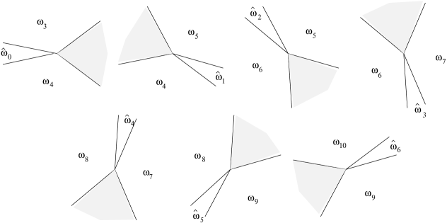
Figure 5.1. Domains $\omega_{m}$, $\hat{\omega}_{m-3}$ and $\omega_{m+1}$ for the algebraic asymptotic behavior of tritronquée Type I solutions for $t=0$. The sectors of the elliptic asymptotic behavior are shown in grey.

5.4.2. Type II tritronquée solutions

There exist seven intersections $U_{m}(x,t)$ of the families $\hat{u}_{m-4}(x,t)$, $u_{m}(x,t)$ and $\hat{u}_{m-3}(x,t)$. These 0-parameter solutions correspond to the Stokes multipliers

$$s_{m-2}=s_{m-1}=s_{m+1}=s_{m+2}=0,\quad s_{m+3}=s_{m-3}=s_{m}=-i,$$

and have the asymptotics

$$U_{m}(x,t)=\\ =\begin{cases}\hat{u}^{(m-4)}(x,t)-(-1)^{m}\frac{1}{2\sqrt{\pi}}(-F^{\prime\prime}(\lambda_{3}))^{-1/2}e^{2F(\lambda_{3})}(1+{\mathcal{O}}(x^{-1/6})),\\ u^{(m)}(x,t),\\ \hat{u}^{(m-3)}(x,t)+(-1)^{m}\frac{1}{2\sqrt{\pi}}(-F^{\prime\prime}(\lambda_{1}))^{-1/2}e^{2F(\lambda_{1})}(1+{\mathcal{O}}(x^{-1/6})),\\ \hat{u}^{(m)}(x,t)-(-1)^{m}\frac{1}{2\sqrt{\pi}}(-F^{\prime\prime}(\lambda_{1}))^{-1/2}e^{2F(\lambda_{1})}(1+{\mathcal{O}}(x^{-1/6}))\\ -(-1)^{m}\frac{1}{2\sqrt{\pi}}(-F^{\prime\prime}(\lambda_{3}))^{-1/2}e^{2F(\lambda_{3})}(1+{\mathcal{O}}(x^{-1/6})),\end{cases}\\ \hfill(x,t)\in\hat{\omega}_{m-4}\cup\omega_{m}\cup\hat{\omega}_{m-3}\cup\hat{\omega}_{m},\\ \mathop{\mapsto}_{t=0}\begin{cases}\hat{u}^{(m-4)}(x)-A_{+}i^{m+1}x^{-1/4}e^{(-1)^{m+1}\frac{6}{7}x^{7/6}h_{+}}(1+{\mathcal{O}}(x^{-1/6})),\\ u^{(m)}(x),\\ \hat{u}^{(m-3)}(x)+A_{-}i^{m+1}x^{-1/4}e^{(-1)^{m+1}\frac{6}{7}x^{7/6}h_{-}}(1+{\mathcal{O}}(x^{-1/6})),\\ \hat{u}^{(m)}(x)+A_{-}i^{m}x^{-1/4}e^{(-1)^{m}\frac{6}{7}x^{7/6}h_{-}}(1+{\mathcal{O}}(x^{-1/6}))\\ -A_{+}i^{m+1}x^{-1/4}e^{(-1)^{m+1}\frac{6}{7}x^{7/6}h_{+}}(1+{\mathcal{O}}(x^{-1/6})),\end{cases}\\ \hfill x\in\hat{\omega}_{m-4}\cup\omega_{m}\cup\hat{\omega}_{m-3}\cup\hat{\omega}_{m}.$$ (5.15)

In Figure 5.2, we present the domains for the algebraic asymptotic behavior of the tritronquée solutions $U_{m}(x)$ of Type II at $t=0$.

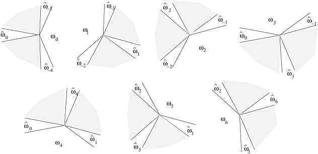
Figure 5.2. Domains $\hat{\omega}_{m}$, $\hat{\omega}_{m-4}$, $\omega_{m}$ and $\hat{\omega}_{m-3}$ for the algebraic asymptotic behavior of tritronquée Type II solutions at $t=0$. The sectors of the elliptic asymptotic behavior are shown in grey.

The solution $U_{0}(x,t)$ real on the real line, with the algebraic asymptotics as $x\to\pm\infty$ was found in [26] for $t=0$ using the isomonodromic deformation approach. The fact that this solution is regular on the real line for any $t$ was proved in [13].

In Figure 5.3, we present the domains $\hat{\omega}_{0}$, $\hat{\omega}_{-4}$, $\omega_{0}$ and $\hat{\omega}_{-3}$ for the algebraic asymptotic behavior of the real and regular on the real line solution $U_{0}(x,t)$ as $t\to\mp\infty$ in the complex plane of the scaled variable $x|t|^{-3/2}$.

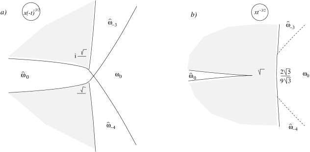
Figure 5.3. The pole-free domains $\hat{\omega}_{0}$, $\hat{\omega}_{-4}$, $\omega_{0}$ and $\hat{\omega}_{-3}$ of the solution $U_{0}(x,t)$ in the plane of the scaled variable $x|t|^{-3/2}$: a) as $t\to-\infty$; b) as $t\to+\infty$. The sectors of the elliptic asymptotic behavior are shown in grey.

Observe some remarkable properties of the domains.

As $t\to-\infty$, two domains of the elliptic behavior are separated by a domain for the algebraic asymptotic behavior. In some neighborhood of the vertices $x=\pm i\tfrac{2\sqrt{2}}{3}(-t)^{3/2}$, the asymptotics of $U_{0}(x,t)$ is given in terms of the tritronquée solutions of the first Painlevé equation P${}_{\mbox{\rm\scriptsize I}}$.

As $t\to+\infty$, the sectors of the algebraic asymptotic behavior of $U_{0}(x,t)$ are separated by a connected domain of the elliptic behavior, and in a neighborhood of the vertex $x=-2\sqrt{3}\,t^{3/2}$, the solution $U_{0}(x,t)$ is approximated by the Hastings-McLeod solution of the second Painlevé equation P${}_{\mbox{\rm\scriptsize II}}$ [11]. More details on the pole distribution in the elliptic sector as $t\to+\infty$ can be found in [17].

In Figure 5.4, we present the domains $\omega_{3}$, $\hat{\omega}_{0}$ and $\omega_{4}$ for the algebraic asymptotic behavior of the real on the real line solution $V_{0}(x,t)$ as $t\to\mp\infty$ in the complex plane of the scaled variable $x|t|^{-3/2}$.

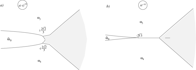
Figure 5.4. The pole-free domains $\omega_{3}$, $\hat{\omega}_{0}$ and $\omega_{4}$ of the solution $V_{0}(x,t)$ in the plane of the scaled variable $x|t|^{-3/2}$: a) as $t\to-\infty$; b) as $t\to+\infty$. The sectors of the elliptic asymptotic behavior are shown in grey.

In the neighborhood of the vertex $x=\tfrac{2\sqrt{2}}{3}\,t^{3/2}$ as $t\to+\infty$ and in the neighborhoods of the vertices $x=\pm i\tfrac{2\sqrt{2}}{3}(-t)^{3/2}$ as $t\to-\infty$, the asymptotics of $V_{0}(x,t)$ is given in terms of the tritronquée solutions of the first Painlevé equation P${}_{\mbox{\rm\scriptsize I}}$.

5.5. Quasi-linear Stokes phenomenon

The notion of the quasi-linear Stokes phenomenon introduced in [25] refers to an exponentially small difference between two analytic functions with identical formal power expansions in a common sector of the complex plane. In the case of equation P${}_{\mbox{\rm\scriptsize I}}^{2}$ at bounded values of $t$, all solutions $u^{(m)}(x,t)$ and $\hat{u}^{(n)}(x,t)$ have the same leading order asymptotics $u_{f}(x,t)\sim-\sqrt[3]{6}x^{1/3}$ as $x\to\infty$ in certain sectors of the complex $x$ plane and the very same complete formal asymptotic power series expansion, $u_{f}(x,t)=\sum_{n=0}^{\infty}a_{n}x^{-\frac{1}{3}(n-1)}$, uniquely determined by the leading order coefficient $a_{0}=-\sqrt[3]{6}$ using the recurrence relation below (the sum is assumed to be empty if the upper bound is less than the lower one),

$$u_{f}(x,t)=\sum_{n=0}^{\infty}a_{n}x^{-\frac{1}{3}(n-1)},\quad a_{k}=\begin{cases}0,\quad k<0,\\ -\sqrt[3]{6},\quad k=0,\\ P_{k}(a_{n<k}),\quad k>0,\end{cases}\\ P_{k}(a_{n<k})=a_{0}^{-2}\Bigl{(}2ta_{k-2}-\sum_{m=2}^{k-2}\tfrac{1}{3}a_{0}a_{m}a_{k-m}-\sum_{n=2}^{k-1}\sum_{m=0}^{k-n}\tfrac{1}{3}a_{n}a_{m}a_{k-n-m}\\ -\sum_{n=0}^{k-7}\tfrac{(n-1)(k+n-4)}{108}a_{n}a_{k-n-7}-\tfrac{(k-15)(k-12)(k-9)(k-6)}{9720}a_{k-14}\Bigr{)},\quad k>0.\quad$$ (5.16)

If $t=0$, the formal series simplifies,

$$u_{f}(x,t)=\sum_{n=0}^{\infty}b_{n}x^{-\frac{1}{3}(7n-1)},\quad b_{0}=-\sqrt[3]{6},\quad b_{1}=\tfrac{1}{36},\quad\\ b_{n+1}=-\sum_{m=0}^{n-1}\tfrac{1}{3}b_{0}^{-1}b_{n-m}b_{m+1}-\sum_{l=0}^{n-1}\sum_{m=0}^{n-l}\tfrac{1}{3}b_{0}^{-2}b_{n-m-l}b_{l+1}b_{m}\\ -\sum_{m=0}^{n}\tfrac{(7m-1)(7n+7m+3)}{3^{3}\cdot 2^{2}}b_{0}^{-2}b_{m}b_{n-m}-\tfrac{(7n-8)(7n-5)(7n-2)(7n+1)}{5\cdot 3^{5}\cdot 2^{3}}b_{0}^{-2}b_{n-1},\quad n\geq 1.$$ (5.17)

The exponentially small differences between the solutions $u^{(m)}(x)$ and $\hat{u}^{(n)}(x)$ with the identical expansions (5.16) can be extracted from the asymptotics of the bitronquée (5.11), (5.13) or tritronquée (5.14), (5.15) solutions above. Indeed, these formulas can be understood as the mutual analytic continuations of $u_{m}(x)$ and $\hat{u}_{n}(x)$ into adjacent sectors of the complex $x$ plane. For instance, taking into account the relation $s_{m-2}+s_{m}=-i$ in (5.10), the asymptotics (5.11) is rewritten as

$$\hat{u}^{(m-3)}(x,t)-u^{(m)}(x,t)=\tfrac{(-1)^{m+1}}{2\sqrt{\pi}}(F^{\prime\prime}(\lambda_{1}))^{-\frac{1}{2}}e^{-2F(\lambda_{1})}(1+{\mathcal{O}}(x^{-1/6}))\\ \mathop{\mapsto}_{t=0}A_{-}i^{m-1}x^{-\frac{1}{4}}e^{(-1)^{m+1}\frac{6}{7}x^{7/6}h_{-}}(1+{\mathcal{O}}(x^{-1/6})),\quad x\in\omega_{m}\cup\hat{\omega}_{m-3}.$$ (5.18)

Similarly, (5.13) with the use of the relation $s_{m+1}+s_{m+3}=-i$ from (5.12) yield

$$u^{(m+1)}(x,t)-\hat{u}^{(m-3)}(x,t)=\tfrac{(-1)^{m+1}}{2\sqrt{\pi}}(F^{\prime\prime}(\lambda_{3}))^{-\frac{1}{2}}e^{-2F(\lambda_{3})}(1+{\mathcal{O}}(x^{-1/6}))\\ \mathop{\mapsto}_{t=0}A_{+}i^{m}x^{-\frac{1}{4}}e^{(-1)^{m}\frac{6}{7}x^{7/6}h_{+}}(1+{\mathcal{O}}(x^{-1/6})),\quad x\in\omega_{m+1}\cup\hat{\omega}_{m-3}.$$ (5.19)

6. Coefficient asymptotics for $t=o(x^{2/3})$

The intimate relation between the Stokes phenomenon and the coefficient asymptotics in the formal solutions to linear and nonlinear ODEs is well explained in [18], see also [25, 29]. The most recent developments of the coefficient asymptotics evaluation method including numerical tests can be found in [21]. Here we develop similar ideas for the formal expansion (5.16) which admits an asymptotic interpretation for $tx^{-2/3}\to 0$ as $x\to\infty$. Our approach follows the above mentioned papers and significantly differs from the method developed in the framework of the resurgent analysis, see e.g. [32, 34] and references mentioned therein.

Introduce the piece-wise meromorphic function as the collection of the 14 tritronquée solutions defined above,

$$W(\tau,t)=\begin{cases}u^{(m)}(\tau^{3},t),\quad\arg\tau\in[-\frac{\pi}{7}+\frac{1}{3}\beta_{0}+\frac{2\pi}{7}m,\frac{\pi}{7}-\frac{1}{3}\beta_{0}+\frac{2\pi}{7}m],\\ \hat{u}^{(m-3)}(\tau^{3},t),\quad\arg\tau\in[\frac{\pi}{7}-\frac{1}{3}\beta_{0}+\frac{2\pi}{7}m,\frac{\pi}{7}+\frac{1}{3}\beta_{0}+\frac{2\pi}{7}m],\end{cases}\\ \beta_{0}=\tfrac{3}{7}\arctan\tfrac{1}{\sqrt{5}},\quad m=0,1,\dots,6.$$ (6.1)

This function has the uniform asymptotic expansion as $\tau\to\infty$,

$$W(\tau,t)=\sum_{n=0}^{M}a_{n}(t)\tau^{-n+1}+{\mathcal{O}}(\tau^{-M}),$$

with the coefficients $a_{n}$ defined in (5.16). Note that $W(\tau)$ can have a finite number of poles all of which are located in the interior of the disc $|\tau|<r_{0}$.

Integrating the product

$$\tau^{N-2}W(\tau,t)=P_{N-1}(\tau,t)+a_{N}(t)\tau^{-1}+{\mathcal{O}}(\tau^{-2}),\quad P_{N-1}(\tau,t)=\sum_{n=0}^{N-1}a_{n}\tau^{N-1-n},$$

over a counter-clock-wise oriented circle of large radius $|\tau|=r\gg r_{0}$, we find

$$a_{N}(t)=\tfrac{1}{2\pi i}\oint_{C_{r}}\tau^{N-2}W(\tau,t)\,d\tau+{\mathcal{O}}(r^{-1}).$$

Contracting the arcs of the circle $C_{r}$ in the interior of the sectors in (6.1) to the circle of radius $|\tau|=r_{0}$, and using (5.19), (5.18), we compute

$$a_{N}(t)=\tfrac{1}{2\pi i}\sum_{m=0}^{6}\int_{e^{-i\frac{1}{3}\alpha_{0}+i\frac{2\pi}{7}m}(r_{0},r)}\tau^{N-2}(\hat{u}^{(m-4)}(\tau^{3},t)-u^{(m)}(\tau^{3},t))\,d\tau\\ +\tfrac{1}{2\pi i}\sum_{m=0}^{6}\int_{e^{i\frac{1}{3}\alpha_{0}+i\frac{2\pi}{7}m}(r_{0},r)}\tau^{N-2}(u^{(m)}(\tau^{3},t)-\hat{u}^{(m-3)}(\tau^{3},t))\,d\tau\\ +\tfrac{1}{2\pi i}\oint_{C_{r_{0}}}\tau^{N-2}W(\tau,t)\,d\tau+{\mathcal{O}}(r^{-1})=\\ =-\tfrac{1}{4\pi^{3/2}i}\sum_{m=0}^{6}e^{i\frac{2\pi}{7}Nm}\int_{e^{-i\frac{1}{3}\alpha_{0}}(r_{0},r)}\tau^{N-2}(F^{\prime\prime}(\lambda_{3}))^{-\frac{1}{2}}e^{-2F(\lambda_{3})}(1+{\mathcal{O}}(\tau^{-\frac{1}{2}}))\bigr{|}_{\genfrac{}{}{0.0pt}{}{x\mapsto\tau^{3}}{t\mapsto t\exp(-i18\pi m/7)}}\,d\tau\\ +\tfrac{1}{4\pi^{3/2}i}\sum_{m=0}^{6}e^{i\frac{2\pi}{7}Nm}\int_{e^{i\frac{1}{3}\alpha_{0}}(r_{0},r)}\tau^{N-2}(F^{\prime\prime}(\lambda_{1}))^{-\frac{1}{2}}e^{-2F(\lambda_{1})}(1+{\mathcal{O}}(\tau^{-\frac{1}{2}}))\bigr{|}_{\genfrac{}{}{0.0pt}{}{x\mapsto\tau^{3}}{t\mapsto t\exp(-i18\pi m/7)}}\,d\tau\\ +{\mathcal{O}}(r_{0}^{N-1})+{\mathcal{O}}(r^{-1}).$$

As $xt^{-3/2}\to\infty$, we find the asymptotics

$$F(\lambda_{1,3})=\tfrac{1}{2}\tfrac{6}{7}x^{7/6}h_{\mp}\pm i(\tfrac{15}{2})^{1/4}e^{\mp i\frac{3}{2}\arctan\frac{1}{\sqrt{5}}}tx^{1/2}+{\mathcal{O}}(x^{-1/6}),\\ (F^{\prime\prime}(\lambda_{1,3}))^{-1/2}=\pm i2\sqrt{\pi}A_{\mp}x^{-1/4}(1+{\mathcal{O}}(tx^{-2/3})),\hfill$$ (6.2)

where $h_{\pm}$ and $A_{\pm}$ are defined in (4.30), letting $r=\infty$ and using conventional steepest descent analysis of the integrals,

$$a_{N}(t)=\tfrac{1}{2\pi}\sum_{\sigma\in\{+,-\}}A_{-\sigma}\sum_{m=0}^{6}e^{i\frac{2\pi}{7}Nm}\int_{e^{\sigma i\frac{1}{3}\alpha_{0}}(r_{0},\infty)}\exp\bigl{\{}-\tfrac{6}{7}\tau^{7/2}h_{-\sigma}\\ -\sigma i2^{3/4}15^{1/4}e^{-\sigma i\frac{3}{2}\arctan\frac{1}{\sqrt{5}}}te^{-i\frac{18\pi}{7}m}\tau^{3/2}+(N-\tfrac{11}{4})\ln\tau\bigr{\}}(1+{\mathcal{O}}(\tau^{-\frac{1}{2}}))\,d\tau\\ +{\mathcal{O}}(r_{0}^{N-1})=\\ =\tfrac{1}{2\sqrt{7\pi}}e^{(\frac{2}{7}N-1)\ln(N-\frac{11}{4})}e^{-(\frac{2}{7}N-\frac{11}{14})}\bigl{(}5^{\frac{1}{2}}3^{\frac{17}{6}}2^{\frac{11}{6}}\bigr{)}^{-\frac{1}{7}N+\frac{1}{4}}\times\\ \times\sum_{\sigma\in\{+,-\}}A_{-\sigma}e^{\sigma i(\frac{1}{7}N-\frac{1}{4})\arctan\frac{1}{\sqrt{5}}}\sum_{m=0}^{6}e^{i\frac{2\pi}{7}Nm-itN^{3/7}b_{\sigma,m}}(1+{\mathcal{O}}(N^{-1/7}))+{\mathcal{O}}(r_{0}^{N-1}),\\ b_{\sigma,m}=\sigma 5^{\frac{1}{7}}3^{-\frac{5}{14}}2^{\frac{5}{14}}e^{-\sigma i\frac{9}{7}\arctan\frac{1}{\sqrt{5}}}e^{-i\frac{18\pi}{7}m},\quad N\to\infty.$$ (6.3)

Observe the agreement of (6.3) with the triviality of the coefficients $a_{n}$ unless $n\equiv 0\mod(7)$ at $t=0$, see (5.17).

7. Numerical evaluation of regular solutions to the P${}_{\mbox{\rm\scriptsize I}}^{2}$ equation

In this section we present a numerical approach to pole-free solutions to P${}_{\mbox{\rm\scriptsize I}}^{2}$ to illustrate some of the results of the previous sections.

7.1. Numerical Methods

We will study here the special solutions to the equation P${}_{\mbox{\rm\scriptsize I}}^{2}$ called tritronquée in the previous sections. The type I solution denoted by $V_{0}(x,t)$ is similar to the tritronquée solution of the P${}_{\mbox{\rm\scriptsize I}}$ equation (see [16] for figures). The type II solution denoted by $U_{0}(x,t)$ is real and pole-free on the real axis. Here we are interested in the sectors of the complex $x$ plane where these solutions are regular and exhibit the algebraic asymptotic behavior,

$$u\sim-\sqrt[3]{6}\,x^{1/3}\quad\mbox{ as }\quad|x|\to\infty,$$ (7.1)

in different sectors of the complex plane, see Figures 5.2, 5.3 and Figures 5.1, 5.4.

In the literature, it is possible to find various numerical approaches to solutions of Painlevé-type equations. For instance, if a Painlevé transcendent can be represented in terms of a Fredholm determinant, it is possible to apply the methods of [3]. Unfortunately such an expression does not yet exist for the solution $U_{0}(x,t)$.

It is known [35] that equation P${}_{\mbox{\rm\scriptsize I}}^{2}$ possesses the Painlevé property, thus all its solutions are meromorphic functions of $x$ and $t$. A convenient approach to study numerically meromorphic functions are Padé approximants, see [19] for the tritronquée solution of P${}_{\mbox{\rm\scriptsize I}}$. A disadvantage of this approach is a lack of error control for the Padé approximants. It might be more promising to solve numerically the Riemann-Hilbert problem as in [31].

Here we concentrate on the pole free sectors for solutions to P${}_{\mbox{\rm\scriptsize I}}^{2}$ as in [22]. The idea of our numeric method is the formulation of a boundary value problem for P${}_{\mbox{\rm\scriptsize I}}^{2}$ on a finite interval consistent with the asymptotic condition (7.1). First we construct the series (5.16) in the form

$$u=Y+\sum_{n=1}^{\infty}c_{n}Y^{-n},\quad Y=-\sqrt[3]{6}\,x^{1/3}.$$ (7.2)

We find the non-zero coefficients $c_{1}=2t$, $c_{2}=c_{3}=c_{4}=0$, $c_{5}=-\tfrac{8}{3}t^{3}$, $c_{6}=1$, $c_{7}=\tfrac{16}{3}t^{4}$, $c_{8}=-\tfrac{10}{3}t$, $c_{9}=0$, $c_{10}=-\tfrac{28}{3}t^{2}$, $c_{11}=-\tfrac{256}{9}t^{6}$, $c_{12}=96t^{3}$, $c_{13}=\tfrac{640}{9}t^{7}-21$, $c_{14}=-\tfrac{1936}{9}t^{4}$, …We truncate this formal series at the $n$-th term for which $|c_{n}Y^{-n}|<10^{-6}$ at the boundary of the computational domain $x\in[x_{l},x_{r}]$. At the values $x_{l}$ and $x_{r}$, the truncated series (7.2) provides us with the necessary boundary data, and we obtain a boundary value problem which replaces the original asymptotic value problem.

The standard approach to boundary value problems for an ODE is to choose a suitable discretization of the dependent variable, see for instance [38, 4]. This leads to an approximation of the derivatives in terms of so called differentiation matrices. In [22], we used a collocation method with cubic splines distributed as bvp4 with Matlab. In [23], we applied a Chebyshev collocation method on Chebyshev collocation points $x_{j}$, $j=0,\ldots,N_{c}$. This is related to an expansion of the solution in terms of Chebyshev polynomials. Since the derivative of a Chebyshev polynomial can be again expressed in terms of a linear combination of Chebyshev polynomials, this leads to the well known Chebyshev differentiation matrices, see for instance [38]. The P${}_{\mbox{\rm\scriptsize I}}^{2}$ equation (1.1) is thus replaced by $N_{c}+1$ algebraic equations. The boundary data are included via the so-called $\tau$-method: the equations for $j=0,1,N_{c}-1,N_{c}$ are replaced by the boundary conditions following from (7.2).

The resulting system of algebraic equations is solved using Newton’s method with the initial iterate $u=-6^{1/3}x/(1+x^{2})^{1/3}$, a smooth function which satisfies for large $x$ the asymptotic conditions, or a linear interpolation between the boundary data. For highly oscillatory solutions, the iteration in general fails to converge. Thus we use a Newton-Armijo method, see [30, 1] and references therein for details.

The normal Newton iteration for the solution of an equation $F(v_{n})=0$ takes the form

$$v_{n+1}=v_{n}-(\mbox{Jac}F(v_{n}))^{-1}F(v_{n}),$$

where $\mbox{Jac}F$ is the Jacobian of $F$. The basic idea is to check at each step of the iteration whether the new iterate $v_{n+1}$ satisfies the equation better than the previous one, i.e. whether $\|F(v_{n+1})\|<\|F(v_{n})\|$. If this is not the case, a so called line search is performed, i.e. the new iterate is taken as $v_{n+1}=v_{n}-\lambda(\mbox{Jac}F(v_{n}))^{-1}F(v_{n})$ where $0<\lambda<1$. In practice we choose a quadratic model for $F(v_{n-1})$, $F(v)$ and $F(v_{n+1})$ to optimize the choice of $\lambda$ as discussed in [30]. For highly oscillatory solutions it can happen that there is no $\lambda$ satisfying the condition. In this case we take a $\lambda$ of the order of $10^{-5}$ and continue the iteration. In the shown examples below, the solution will converge after some iterations even if the line search failed at one point. The precision is mainly limited by the conditioning of the Chebyshev differentiation matrix which is of the order of $N_{c}^{2}$, see the discussion in [38] for the second order differentiation matrices. We use here $N_{c}=512$ or $N_{c}=1024$ and reach an accuracy of the order of $10^{-6}$.

To study solutions in the complex plane, i.e. as a holomorphic function of the complex coordinate $x$ in a given sector, we proceed as in [16]: we determine the solution as discussed above on a line given by $x=\xi e^{i\phi}$ with $\xi,\phi\in\mathbb{R}$. This solution is then used as the boundary data for the two-dimensional Laplace equation which is solved as discussed in [16, 38]. Due to the coordinate singularity of the solution for $|x|=0$, the precision is much lower than for the solution on a line in the complex plane and serves mainly for visualization.

7.2. Type I tritronquée solutions

We first study the type I tritronquée solution $V_{0}$ which is a straightforward generalization of the well known real tritronquée solution of P${}_{\mbox{\rm\scriptsize I}}$ studied numerically in [16, 19]. This similarity allows us to concentrate on the most interesting details.

We first determine the solution on the imaginary axis where we put $x=\exp(i\phi)\xi$, $\xi\in\mathbb{R}$ and $\phi=5\pi/2$. We get the solution shown in Fig. 7.1

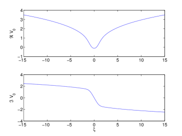
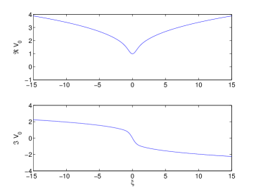
Figure 7.1. Solution $V_{0}(x,t)$ to P${}_{\mbox{\rm\scriptsize I}}^{2}$ satisfying the asymptotic condition (7.1) for $x=\exp(i\phi)\xi$, $\xi\in\mathbb{R}$ and $\phi=5\pi/2$; on the left for $t=-1$, on the right for $t=0$.

If we consider the same solution for $t=0$ on a parallel to the imaginary axis, $x=\exp(i\phi)\xi+b$, $\xi,b\in\mathbb{R}$ and $\phi=5\pi/2$, the solution becomes more peaked for positive $b$ as can be seen in Fig. 7.2. It appears as if this peak will become a pole for larger $b$, but this cannot be determined with the used numerical methods.

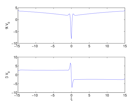
Figure 7.2. Solution $V_{0}(x,t)$ to P${}_{\mbox{\rm\scriptsize I}}^{2}$ satisfying the asymptotic condition (7.1) for $t=0$ and $x=\exp(i\phi)\xi+b$, $\xi\in\mathbb{R}$ and $\phi=5\pi/2$ for $b=5.5$.

If one changes the angle $\phi$ for $b=0$, the solution will become trigonometric on the lines with $\phi=15\pi/7+3/7\arctan(1/\sqrt{5})\sim 0.6290+2\pi$. This behavior is illustrated in Fig. 7.3 for a slightly larger $\phi$.

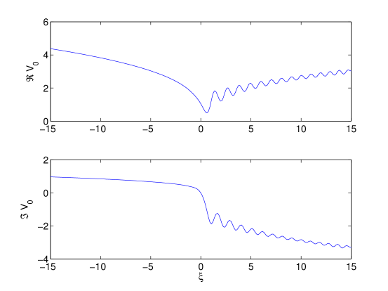
Figure 7.3. Solution $V_{0}(x,t)$ to P${}_{\mbox{\rm\scriptsize I}}^{2}$ satisfying the asymptotic condition (7.1) for $t=0$ and $x=\exp(i\phi)\xi$, $\xi\in\mathbb{R}$ and $\phi=2\pi+0.6932$.

As in the case of the tritronquée solutions of P${}_{\mbox{\rm\scriptsize I}}$ in [16], it is possible to study the P${}_{\mbox{\rm\scriptsize I}}^{2}$ solution $V_{0}(x,t)$ with the condition (7.1) in the sector of the complex plane with $\mbox{arg}x\in[-\phi,\phi]$ in the cases shown in Figure 7.9. We analytically continue the cubic root not to be branched in the shown sector close to the negative real axis. For $t=0$, one obtains Figure 7.4 for the real part of the solution and Figure 7.5 for its imaginary part. It appears that there are no poles in the shown sectors even for finite $|x|$.

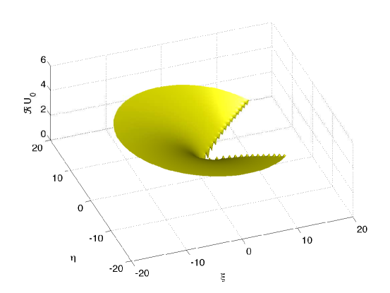
Figure 7.4. Real part of the type I tritronquée solution to the P${}_{\mbox{\rm\scriptsize I}}^{2}$ equation (1.1) with asymptotic condition (7.1) in the complex plane for $t=0$.

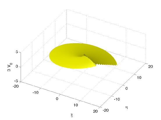
Figure 7.5. Imaginary part of the type I tritronquée solution to the P${}_{\mbox{\rm\scriptsize I}}^{2}$ equation (1.1) with asymptotic condition (7.1) in the complex plane for $t=0$.

7.3. Type II tritronquée solutions

The solution $U_{0}(x,t)$ characterized by the asymptotic behavior (7.1) is real and pole-free on the real line for all $t\in{\mathbb{R}}$ [13]. For large negative $t$, the solution has no oscillations, but they appear for $t\sim 0$, see Figure 7.6.

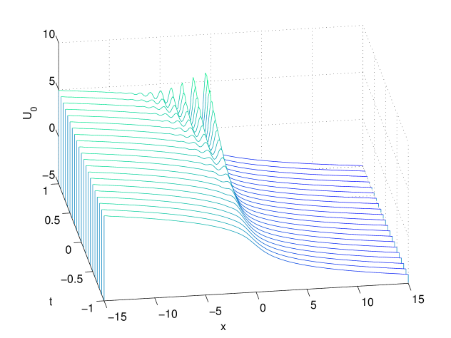
Figure 7.6. Solution $U_{0}(x,t)$ for $x\in\mathbb{R}$ to P${}_{\mbox{\rm\scriptsize I}}^{2}$ satisfying the asymptotic condition (7.1) for several values of $t$.

For positive $t$, the oscillations rapidly develop, see Figure 7.7.

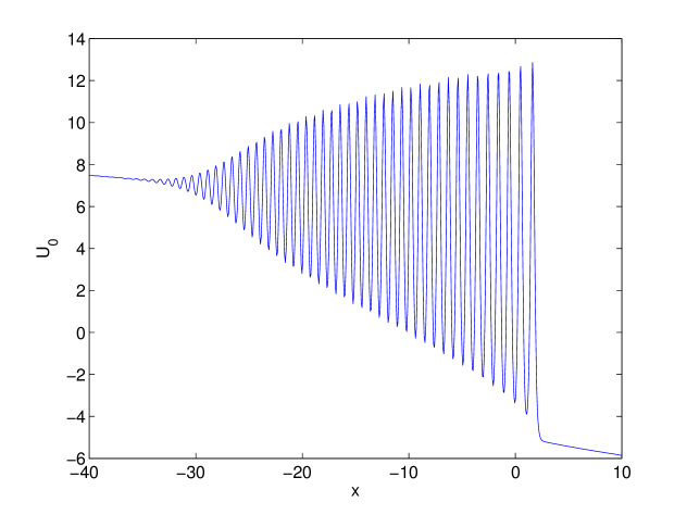
Figure 7.7. Solution $U_{0}(x,t)$ to P${}_{\mbox{\rm\scriptsize I}}^{2}$ for $t=4$.

The location of the oscillations for $t>0$ in Figure 7.6 agrees with the theoretical prediction of the interval $\bigl{(}-2\sqrt{3}\,t^{3/2},\tfrac{2\sqrt{5}}{9\sqrt{3}}t^{3/2}\bigr{)}$, see Figure 5.3 which belongs to the sector of the elliptic asymptotic behavior of $U_{0}(x,t)$. This indicates the presence of poles in the complex plane approaching the real axis [8],[20].

To test this we solve P${}_{\mbox{\rm\scriptsize I}}^{2}$ with the asymptotic condition (7.1) on a line parallel to the real axis parameterized by $x=\xi+b$ with $\xi\in\mathbb{R}$ and $b\in i\mathbb{R}$. We vary $b$ gradually from zero and stop when observing a strong increase in the absolute value of the solution. This can be seen in Figure 7.8 for two values of $t$. For positive $t$, the presumed singularity moves very close to the real axis.

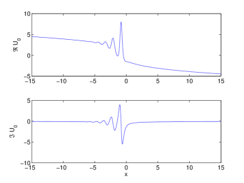
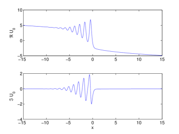
Figure 7.8. Solution to the P${}_{\mbox{\rm\scriptsize I}}^{2}$ equation (1.1) with asymptotic condition (7.1) on a line parallel to the real axis, $x=\xi+b$, $\xi\in\mathbb{R}$; on the left the case $t=0$ and $b=0.8i$, on the right $t=1$ and $b=0.1i$. We are plotting the maximum values of $|b|$ for which the numerical code does not break. In the second case $|b|$ is smaller because the poles of the solution are approaching the real axis as $t$ is getting bigger.

In the same way it is possible to study P${}_{\mbox{\rm\scriptsize I}}^{2}$ (1.1) with the condition (7.1) on lines in the complex plane given by $x=e^{i\phi}\xi$ with $\xi,\phi\in\mathbb{R}$ with the goal to identify numerically the sectors in the complex plane, where the solution has no poles.

In Figure 7.9 we show the solution for $t=0$ close to the real axis for $\phi=0.15$. It can be seen that the amplitude of the oscillations decreases slower than on the real axis. We expect to observe the trigonometric behavior of the solution on the line with $\phi=3/7\arctan(1/\sqrt{5})\sim 0.1802$ for $\xi<0$. The closer one comes to this line, the less reliable the numerical solution is since the asymptotic series yielding after truncation the boundary data converges more and more slowly for a finite value of $|x|$.

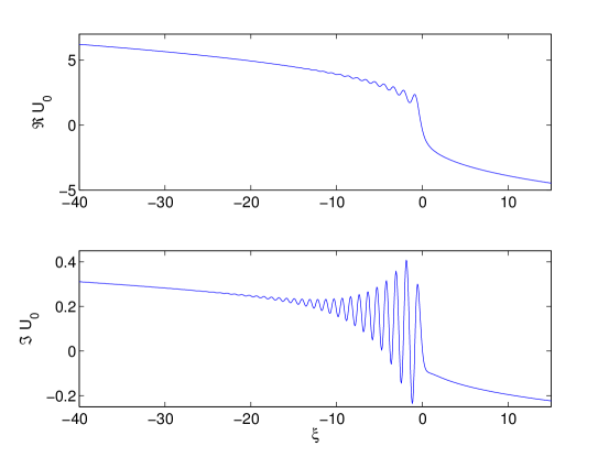
Figure 7.9. Solution to the P${}_{\mbox{\rm\scriptsize I}}^{2}$ equation (1.1) with asymptotic condition (7.1) on a line in the complex plane given by $x=e^{i\phi}\xi$ with $\xi,\phi\in\mathbb{R}$ for $t=0$ and $\phi=0.15$.

As discussed in the previous sections, the regular sector is considerably larger in the vicinity of the positive real axis. In Figure 7.10 we show the solution on the half line $x=\xi e^{i\phi}$ for $\phi=1.5$ and $\xi>0$. As predicted the solution shows oscillations with asymptotically decreasing amplitude close to the line with $\phi=3\pi/7+3/7\arctan(1/\sqrt{5})\sim 1.5266$, the dependence of $U_{0}(x,t)$ on $|x|$ becomes trigonometric. We are able to reach the value $\phi=1.5$. The regular sectors (angles between $\pi-0.18$ and $\pi+.18$ near the negative real axis and between $-1.5$ and $1.5$ near the positive real axis) are illustrated in Figures 7.11 and 7.12 below. The oscillations near the boundaries of these sectors can be clearly recognized and are even more pronounced for the imaginary part.

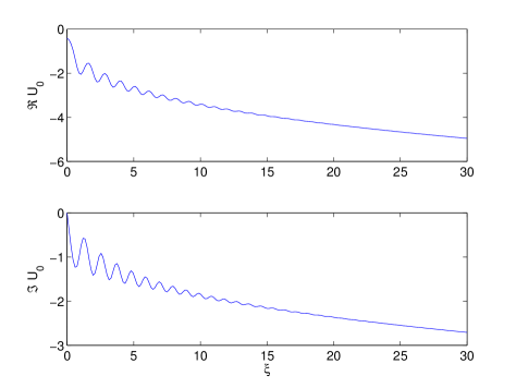
Figure 7.10. Solution to the PI2 equation (1.1) with asymptotic condition (7.1) on a halfline in the complex plane given by $x=e^{i\phi}\xi$ with $\xi>0$ for $t=0$ and $\phi=1.5$.

We again study the P${}_{\mbox{\rm\scriptsize I}}^{2}$ solution with the condition (7.1) in the sectors of the complex plane between $-\phi$ and $\phi$ for the cases shown in Figure 7.9. We analytically continue the cubic root not to be branched in the shown sectors close to the real axis. For $t=0$, one obtains Figure 7.11 for the real part of the solution and Figure 7.12 for the imaginary part. It appears that there are no poles in the shown sectors even for finite $|x|$.

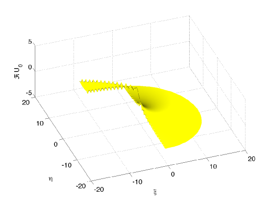
Figure 7.11. Real part of the solution to the P${}_{\mbox{\rm\scriptsize I}}^{2}$ equation (1.1) with asymptotic condition (7.1) in the complex plane for $t=0$.

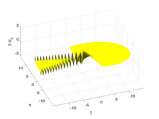
Figure 7.12. Imaginary part of the solution to the P${}_{\mbox{\rm\scriptsize I}}^{2}$ equation (1.1) with asymptotic condition (7.1) in the complex plane for $t=0$.

It was shown in the previous sections, see e.g. (1.3) and (1.4) that the difference type I and type II solutions is exponentially small on the negative real axis. This can be seen in Fig. 7.13. The type II solution shows oscillations close to the origin which are not present for the type I solution, but then they agree in a way that no difference can be seen. In the left part of Fig. 7.13 we therefore show the logarithmic plot of the absolute value of the difference between both solutions which decreases as expected exponentially with increasing $-x$, i.e., lineary in a logarithmic plot until the difference is of the order of the rounding error.

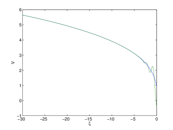
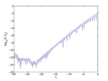
Figure 7.13. Type I and type II solution to the P${}_{\mbox{\rm\scriptsize I}}^{2}$ equation (1.1) with asymptotic condition (7.1) on the negative real axis for $t=0$; on the left the type I solution in blue and the type II solution in green, on the right the difference between both.

References

- [1] L. Armijo, Minimization of functions having Lipschitz continuous first partial derivatives, Pacific J. Math. 16 (1966) no. 1, 1-3.
- [2] J.-P. Berrut, L.N. Trefethen, Barycentric Lagrange Interpolation, SIAM REVIEW 46, No. 3, pp. 501–517 (2004).
- [3] F. Bornemann, On the Numerical Evaluation of Fredholm Determinants, Math. Comp. 79 (2010) 871–915.
- [4] F. Bornemann, T.A. Driscoll and L.N. Trefethen, The Chebop System for Automatic Solution of Differential Equations, BIT 48 (2008) 701–723.
- [5] H. Bateman and A. Erdelyi, Higher Transcendental Functions, McGraw-Hill, NY, 1953.
- [6] P. Boutroux, Recherches sur les transcendantes de M. Painlevé et l’étude asymptotique des équationes differéntielle du second ordre, Ann. Sci. Ec. Norm. Super. (3), 30 (1913) 255–375; 31 (1914) 99-159.
- [7] E. Brézin, E. Marinari and G. Parisi, A non-perturbative ambiguity free solution of a string model, Phys. Lett. B 242 (1990) no. 1, 35-38.
- [8] T. Claeys, Asymptotics for a special solution to the second member of the Painlevé I hierarchy, J. Phys. A: Math. Theor. 43 (2010) 434012 (18pp).
- [9] T. Claeys and T. Grava, Universality of the break-up profile for the KdV equation in the small dispersion limit using the Riemann-Hilbert approach, Commun. Math. Phys. 286 (2009) 979-1009.
- [10] T. Claeys and T. Grava, Critical asymptotic behavior for the Korteweg-de Vries equation and in random matrix theory, arXiv:1210.8352 [math-ph]
- [11] T. Claeys and T. Grava, The KdV hierarchy: universality and a Painlevé transcendent. Int. Math. Res. Not. IMRN 2012, no. 22, 5063-5099.
- [12] T. Claeys, A. Its and I. Krasovsky, Higher-order analogues of the Tracy-Widom distribution and the Painlevé II hierarchy. Comm. Pure Appl. Math. 63 (2010), no. 3, 362–412.
- [13] T. Claeys and M. Vanlessen, Universality of a double scaling limit near singular edge points in random matrix models. Comm. Math. Phys. 273 (2007), no. 2, 499–532.
- [14] B. Dubrovin, On Hamiltonian perturbations of hyperbolic systems of conservation laws, II: universality of critical behavior, Comm. Math. Phys. 267 (2006) 117-139.
- [15] B. Dubrovin, On universality of critical behavior in Hamiltonian PDEs, Geometry, topology, and mathematical physics, (2008) 59–109, Amer. Math. Soc. Transl. Ser. 2, 224, Amer. Math. Soc., Providence, RI, 2008; arXiv:0804.3790[math.AP].
- [16] B. Dubrovin, T. Grava, C. Klein, On universality of critical behaviour in the focusing nonlinear Schrödinger equation, elliptic umbilic catastrophe and the tritronquée solution to the Painlevé-I equation, J. Nonl. Sci. 19(1) (2009) 57–94.
- [17] B. Dubrovin and A. Kapaev, On an isomonodromy deformation equation without the Painlevé property, Russian J. Math. Phys. 21 (2014) no. 1, 9-35; arXiv:1301.7211v2[math.CA].
- [18] A.S. Fokas, A.R. Its, A.A. Kapaev and V.Yu. Novokshenov, Painlevé transcendents: the Riemann-Hilbert approach, Math. Surveys and Monographs, 128, Amer. Math. Soc., 2006.
- [19] B. Fornberg and J.A.C. Weideman, A numerical methodology for the Painlevé equations, J. Comp. Phys. 230 (2011) 5957–5973.
- [20] R. Garifullin, B. Suleimanov, N. Tarkhanov, Phase shift in the Whitham zone for the Gurevich-Pitaevskii special solution of the Korteweg-de Vries equation. Phys. Lett. A 374 (2010), no. 13-14, 1420-1424.
- [21] S. Garoufalidis, A. Its, A. Kapaev and M. Mariño, Asymptotics of the instantons of Painleve I, Int. Math. Res. Not. 2012 (2012) no. 3, 561-606. arXiv:1002.3634v1 [math.CA]
- [22] T. Grava, C. Klein, Numerical study of a multiscale expansion of KdV and Camassa-Holm equation, in: Integrable Systems and Random Matrices, ed. by J. Baik, T. Kriecherbauer, L.-C. Li, K.D.T-R. McLaughlin and C. Tomei, Contemp. Math. 458 (2008) 81-99.
- [23] T. Grava and C. Klein, Numerical study of the small dispersion limit of the Korteweg-de Vries equation and asymptotic solutions, Physica D, 10.1016/j.physd.2012.04.001 (2012).
- [24] E.L. Ince, Ordinary differential equations, Dover, New York, 1956.
- [25] A. R. Its and A. A. Kapaev, Quasi-linear Stokes phenomenon for the second Painlevé transcendent, Nonlinearity 16 (2003) no. 1, 363-386; arXiv:nlin/0108010 [nlin.SI]
- [26] A.A. Kapaev, Weakly nonlinear solutions of equation , J. Math. Sci. 73(4) (1995) 468-481.
- [27] A.A. Kapaev, Monodromy deformation approach to the scaling limit of the Painleve first equation, CRM Proc. Lect. Notes, 32 (2002) 157-179; arXiv:nlin/0105002 [nlin.SI]
- [28] A.A. Kapaev, Monodromy approach to the scaling limits in the isomonodromy systems, Theor. Math. Phys., 137, no. 3 (2003) 1691-1702; arXiv:nlin/0211022 [nlin.SI]
- [29] A. A. Kapaev, Quasi-linear stokes phenomenon for the Painlevé first equation. J. Phys. A: Math. Gen. 37 (2004), no. 46, 11149-11167.
- [30] C. T. Kelley, Iterative methods for linear and nonlinear equations, SIAM, 1995.
- [31] S. Olver, Numerical solution of Riemann-Hilbert problems: Painlevé II, Found. Comput. Maths 11 (2011) 153-179.
- [32] M. Mariño, Nonperturbative effects and nonperturbative definitions in matrix models and topological strings, JHEP 0812 (2008) 114; arXiv:0805.3033 [hep-th].
- [33] G. Moore Geometry of the string equations, Comm. Math. Phys 133 (1990) 261-304.
- [34] R. Schiappa and R. Vaz, The Resurgence of Instantons: Multi-Cuts Stokes Phases and the Painlevé II Equation, arXiv:1302.5138 [hep-th].
- [35] S. Shimomura, Painlevé property of a degenerate Garnier system of (9/2)-type and of a certain fourth order non-linear ordinary differential equation, Ann. Scuola Norm. Sup. Pisa 29 (2000) 1–17.
- [36] B.I. Suleimanov, Solution of the Korteweg-de Vries equation which arises near the breaking point in problems with a slight dispersion. JETP Lett. 58 (1993), no. 11, 849-854.
- [37] B.I. Suleimanov, “Quantizations” of higher hamiltonian analogues of the Painlevé I and Painlevé II equations with two degrees of freedom, arXiv:1204.4006 [nlin.SI].
- [38] L. N. Trefethen, Spectral Methods in MATLAB, SIAM, Philadelphia, PA, 2000.