Matter mixing in aspherical core-collapse supernovae: a search for possible conditions for conveying ⁵⁶Ni into high velocity regions

Abstract

We perform two-dimensional axisymmetric hydrodynamic simulations of matter mixing in aspherical core-collapse supernova explosions of a 16.3 $M_{\odot}$ star with a compact hydrogen envelope. Observations of SN 1987A have provided evidence that ⁵⁶Ni synthesized by explosive nucleosynthesis is mixed into fast moving matter ($\gtrsim$ 3,500 km s^-1) in the exploding star. In order to clarify the key conditions for reproducing such high velocity of ⁵⁶Ni, we revisit matter mixing in aspherical core-collapse supernova explosions. Explosions are initiated artificially by injecting thermal and kinetic energies around the interface between the iron core and the silicon-rich layer. Perturbations of 5% or 30% amplitude in the radial velocities are introduced at several points in time. We found that no high velocity ⁵⁶Ni can be obtained if we consider bipolar explosions with perturbations (5% amplitude) of pre-supernova origins. If large perturbations (30% amplitude) are introduced or exist due to some unknown mechanism in a later phase just before the shock wave reaches the hydrogen envelope, ⁵⁶Ni with a velocity of 3,000 km s^-1 can be obtained. Aspherical explosions that are asymmetric across the equatorial plane with clumpy structures in the initial shock waves are investigated. We found that the clump sizes affect the penetration of ⁵⁶Ni. Finally, we report that an aspherical explosion model that is asymmetric across the equatorial plane with multiple perturbations of pre-supernova origins can cause the penetration of ⁵⁶Ni clumps into fast moving matter of 3,000 km s^-1. We show that both aspherical explosion with clumpy structures and perturbations of pre-supernova origins may be necessary to reproduce the observed high velocity of ⁵⁶Ni. To confirm this, more robust three-dimensional simulations are required.

1. Introduction

Morphologies of supernova explosions is a topic of hot debate. Many observations of supernovae and supernova remnants have indicated an aspherical nature of the supernova explosions. SN 1987A, a supernova occurred in the Large Magellanic Cloud on February 23rd, has provided many interesting features to be explained by astronomers and astrophysicists. Observations of SN 1987A have implied large-scale matter mixing in the supernova explosion from several aspects. Early detection of hard X-ray (Dotani et al., 1987; Sunyaev et al., 1987) and $\gamma$-ray lines from decaying ⁵⁶Co (Matz et al., 1988) have indicated that radioactive ⁵⁶Ni synthesized by explosive nucleosynthesis is mixed into fast moving matter composed of helium and hydrogen. The sudden development of the fine-structure of the H_α line (Bochum event : Hanuschik et al., 1988) implies the existence of a high velocity ($\sim$ 4,700 km s^-1) clump of ⁵⁶Ni with a mass of several 10^-3 $M_{\odot}$ (Utrobin et al., 1995). The observed line profiles of [Fe II] in SN 1987A show that the maximum velocity of ⁵⁶Ni (or its decay products ⁵⁶Co and ⁵⁶Fe) reaches $\sim$ 4,000 km s^-1 and the position of the peak of the flux distribution as a function of Doppler velocity is located in the red-shifted side (Haas et al., 1990; Spyromilio et al., 1990). The shape of the flux distribution is asymmetric across the peak. Modeling the light curve of SN 1987A using one-dimensional radiation hydrodynamics calculations requires the mixing of ⁵⁶Ni into high velocity regions to reproduce the observed features of the light curve (Woosely, 1988; Shigeyama, Nomoto & Hashimoto, 1998; Shigeyama & Nomoto, 1990; Blinnikov et al., 2000; Utrobin, 2004). Shigeyama & Nomoto (1990), Blinnikov et al. (2000), and Utrobin (2004) have insisted that mixing of ⁵⁶Ni into high velocity regions up to 3,000 km s^-1, 4,000 km s^-1, and 2,500 km s^-1, respectively. Therefore, the clear consensus about the maximum velocity of ⁵⁶Ni has not been obtained from modelings the light curve and H_α line. However, at least 4% of total mass of ⁵⁶Ni would have $>$ 3,000 km s^-1 (Haas et al., 1990). In addition to ⁵⁶Ni, mixing of hydrogen into inner cores have been inferred and the minimum hydrogen velocity can be $\lesssim$ 800 km s^-1 (Shigeyama & Nomoto, 1990; Kozma & Fransson, 1998). Asphericity of core-collapse supernova explosions have also been implied from other Type II-P supernovae. Observations of He I lines in the IR band from Type II-P supernovae indicate the mixing of ⁵⁶Ni into the helium regions (SN 1995V: Fassia et al., 1998). Clumped structures of ejecta have been revealed by the observations of metal lines of other Type II supernovae (SN 1988A: Spyromilio 1991, SN 1993J: Spyromilio 1994). Recent optical observations of the inner ejecta of the supernova remnant of SN 1987A have revealed that the morphology of the ejecta is elliptical and the ratio of the major to minor axises of the ejecta is 1.8 $\pm$ 0.17 (Kjær et al., 2010). The three-dimensional structure of supernova remnant Cassiopeia A demonstrates clearly that the ejecta is rather clumpy (Delaney et al., 2010).

Theoretically, there is a growing awareness of multi-dimensional effects in supernova explosion mechanisms. In the context of the neutrino heating mechanism, convection in the neutrino heating layers and standing accretion shock instability (SASI) may result in a globally anisotropic structure inside a supernova shock wave (e.g., Kotake et al., 2006). Magnetohydrodynamic (MHD) simulations of the core-collapse of massive stars (Kotake et al., 2004; Sawai et al., 2005; Burrows et al., 2007; Takiwaki et al., 2009) have demonstrated magnetorotationally driven jetlike explosions. For more detailed descriptions of multi-dimensional effects of supernova explosions, see the recent reviews by (e.g., Kotake et al., 2012; Janka, 2012).

Rayleigh-Taylor (RT) instabilities have been thought to be a promising mechanism to facilitate large-scale matter mixing in supernova explosions. Other hydrodynamic instabilities, such as Richtmeyer-Meshkov (RM) instabilities and Kelvin-Helmholtz (KH) instabilities, may also contribute to the mixing in supernovae along with the RT instability. The condition for the RT instability for a compressible fluid is given by $(dP/dr)\,(d\rho/dr)<0$ (Chevalier, 1979), where $P$ is the pressure, $r$ is the radius, and $\rho$ is the density. Stability analyses of supernova shock wave propagations in a pre-supernova model of SN 1987A using one-dimensional hydrodynamics have depicted that the composition interfaces between the hydrogen- and helium-rich layers (He/H) and that between the helium-rich layer and C+O core (C+O/He) can become unstable against RT instabilities (Ebisuzaki et al., 1989; Benz & Thielemann, 1990).

We note that Arnett et al. (1989) commented on the possible sources of the perturbations for initiating the hydrodynamic instabilities. The authors considered three possibilities. One is thermonuclear shell flashes in the oxygen-rich layer. Second is hydrogen shell burning at the edge of the helium core of a pre-supernova star and which makes a jump in density at the composition interface of He/H. Note that the authors stated that the jump is not significant for RT instabilities. Third is the ‘nickel bubble’, i.e. the heating via decays of ⁵⁶Ni competing with the adiabatic cooling. Two-dimensional hydrodynamic simulations of a pre-collapse star have depicted significant fluctuations (up to 8% in density) due to convective oxygen-shell burning at the edges of a burning shell (Bazán & Arnett, 1998). Recent two-dimensional hydrodynamic simulation of progenitor evolution of a 23 $M_{\odot}$ star demonstrated the growth of instabilities of low-order modes and a large anisotropy in each burning shell (Arnett & Meakin, 2011).

Motivated by the observational evidence of matter mixing in supernovae, two or three-dimensional hydrodynamic simulations have been performed in early papers to investigate the effects of RT instabilities on mixing in shock wave propagations in the progenitor star of SN 1987A (Arnett et al., 1989; Hachisu et al., 1990; Fryxell et al., 1991; Müller et al., 1991; Herant & Benz, 1991; Hachisu et al., 1992). All studies above have combined one-dimensional hydrodynamic simulations of supernova explosions with multi-dimensional simulations of late time evolutions of the shock wave propagations. The explosions have been implemented through some ad hoc ways, e.g. thermal bombs or piston models. However, such simulations have revealed that RT instabilities are insufficient to explain the high velocity metals. The obtained maximum velocity of ⁵⁶Ni is $\sim$ 2,000 km s^-1 at 90 day after the explosion using a two-dimensional smoothed particle hydrodynamic (SPH) code (Herant & Benz, 1991). Herant & Benz (1992) referred to this gap between observations and models as the ‘nickel discrepancy’. Herant & Benz (1992) suggested that premixing in regions of the inner 1.5 $M_{\odot}$ above the mass cut is required to reproduce the high velocity wings of the [Fe II] line profiles.

Explosive nucleosynthesis in jetlike explosions have been investigated in several papers (Nagataki et al., 1997, 2003, 2006; Fujimoto et al., 2007, 2008; Ono et al., 2009; Winteler et al., 2012; Ono et al., 2012). In the context of jetlike explosions, matter mixing in mildly asymmetric explosions of the progenitor star of SN 1987A with monochromatic perturbations have been investigated (Yamada & Sato, 1991; Nagataki et al., 1998b; Nagataki, 2000). Yamada & Sato (1991) concluded that an asymmetric explosion with initial perturbations of 30% amplitude causes strong mixing and high velocity innermost metals ($\sim 4,000$ km s^-1). Nagataki et al. (1998b) and Nagataki (2000) have reproduced the high velocity component of ⁵⁶Ni ($\sim 3,000$ km s^-1) and line profiles of [Fe II] observed in SN 1987A by a mildly aspherical supernova explosion model with large monochromatic perturbations (amplitude of $30\%$). Additionally, Nagataki (2000) suggested that the strong alpha-rich freeze-out in a jetlike explosion is favored to explain the amount of ⁴⁴Ti in SN 1987A. Nagataki et al. (1998a) applied a high ratio of ⁴⁴Ti/⁵⁶Ni in an asymmetric core-collapse explosion to Cassiopeia A. Note that recently, direct-escape (Hard X-ray) emission lines from the decay of ⁴⁴Ti have been detected (Grebenev et al., 2012) in the remnant of SN 1987A and the mass of ⁴⁴Ti is estimated to be (3.1$\pm$0.8)$\times$10^-4 $M_{\odot}$. In Yamada & Sato (1991), Nagataki et al. (1998b), and Nagataki (2000), the resolutions of the simulations are rather low and they have not taken into account the effects of fallback of the ejecta. In Nagataki et al. (1998b), large perturbations of 30% amplitude are introduced when the shock front reaches the composition interface of He/H. However, as the author noted, such large perturbations should be introduced only in the explosion itself. Hungerford et al. (2003) and Hungerford et al. (2005) have investigated the effects of aspherical explosions on the $\gamma$-ray lines using a three-dimensional SPH code. The authors have shown that aspherical explosions change significantly the velocity distribution of ⁵⁶Ni compared to that in spherical explosions, and aspherical models may reproduce mixing of ⁵⁶Ni into the edge of hydrogen and red-shifted [Fe II] lines. Couch et al. (2009) performed two-dimensional simulations of bipolar, jetlike explosions of Type II supernovae using an adaptive mesh refinement (AMR) hydrodynamic code and commented on the observational features of jetlike explosions against those associated to Type II-P supernovae. Recently, Ellinger et al. (2012) studied RT mixing in a series of aspherical core-collapse supernova explosions using a three-dimensional SPH code and the authors discussed the sizes of the arising clumps.

Joggerst et al. (2009) investigated matter mixing due to RT instabilities and fallback in spherical core-collapse supernova explosions of solar- and zero-metallicity stars with a two-dimensional AMR code. The results depict that the growth of RT instabilities are significantly reduced in the zero-metallicity stars which are compact blue supergiants. Joggerst et al. (2010a) examined RT mixing in spherical supernova explosions of rotating zero-metallicity and metal-poor stars. The rotating zero-metallicity stars end their lives as red supergiants in contrast to non-rotating ones. Thus, more mixing and less fallback are expected in rotating zero-metallicity stars than that in non-rotating ones. Three-dimensional simulations of RT mixing in supernova explosions of rotating zero-metallicity and metal-poor stars indicate (Joggerst et al., 2010b) that the degree of mixing at the ends of simulation time does not differ much from that in the two-dimension case.

Kifonidis et al. (2003) and Kifonidis et al. (2006) have investigated matter mixing in neutrino-driven core-collapse supernova explosions aided by convection and SASI using AMR hydrodynamic codes. The authors have found that if the shock wave has only small-scale deviations from spherical symmetry (high-order modes), no high velocity ⁵⁶Ni clump should be expected. On the other hand, a globally aspherical explosion (low-order modes, $l$ = 1, 2) with a relatively high explosion energy (2 $\times$ 10⁵¹ erg) causes strong RM instabilities at the composition interface of He/H and makes clumps of metals penetrate into a dense helium shell before the formation of a strong reverse shock. High velocity ⁵⁶Ni clumps ($\sim$ 3,300 km s^-1) are obtained by the globally aspherical explosion. Gawryszczak et al. (2010) re-investigated the study of Kifonidis et al. (2006) using a single computational domain and pointed out that it is difficult to achieve robust conclusions by two-dimensional axisymmetric hydrodynamic codes.

Hammer et al. (2010) performed a three-dimensional simulation of mixing in a neutrino-driven core-collapse supernova explosion of a compact blue star. The authors suggested that in the three-dimensional model, clumps of ejecta feel less drag force than that in the two-dimensional counterparts, and the high velocity iron group elements ($\sim$ 4,500 km s^-1) with a mass of $\sim$ 10^-3 $M_{\odot}$ are reproduced in the three-dimensional model, which cannot be obtained in two-dimension. However, the resolution of the simulation is lower than that of two-dimensional high-resolution studies (e.g., Kifonidis et al., 2006) due to the limitation of computational resources, and the authors also neglected the effects of gravity, i.e., fallback of matter into the compact remnant. More robust calculations are required to conclude such dimensional effects on the high-velocity metals.

As referenced above, there exists only a few models that obtained high velocity ⁵⁶Ni clumps of $\gtrsim$ 3,000 km s^-1. However, even in such models, there are still several drawbacks in those simulations. The resolutions of simulations in Yamada & Sato (1991), Nagataki et al. (1998b), and Nagataki (2000) and the three-dimensional simulation in Hammer et al. (2010) are low compared with recent two-dimensional hydrodynamic simulations on matter mixing in supernovae (e.g., Kifonidis et al., 2006) and some hydrodynamical instabilities may not be captured in their simulations. The non-radial motion of initial explosion models used in Kifonidis et al. (2006) and Gawryszczak et al. (2010) tends to concentrate ejecta into polar regions. However, ejecta motion around polar regions are doubtful in axsymmetric two-dimensional simulation. Therefore, the conditions for reproducing the observed high velocity of ⁵⁶Ni are still unclear. In the present paper, we investigate matter mixing in a series of aspherical core-collapse supernova explosions of a 16.3 $M_{\odot}$ star with a compact hydrogen envelope using a two-dimensional AMR hydrodynamic code in order to clarify the key conditions for reproducing such high velocity of ⁵⁶Ni. To survey a large variety of aspherical explosions, we adopt the stance that explosions are initiated artificially in similar ways as the earlier papers. We revisit RT mixing in mildly aspherical bipolar explosions by introducing initial perturbations at several points in time. We also consider globally anisotropic explosions with clumpy structures by mimicking neutrino-driven core-collapse explosions. The purpose of this paper is to do a comprehensive search for the preferable conditions to explain the the observed high velocity of ⁵⁶Ni. In §2, our numerical methods are described. §3 is devoted to explaining our models in the this paper. We will show our results in §4, and then discuss several important aspects based on the results in §5. Finally, we conclude our study in §6.

2. Numerical method, initial conditions

The computations in this paper are preformed with the adaptive mesh refinement (AMR) hydrodynamic code, FLASH (Fryxell et al., 2000). We use the directionally split Eulerian version of the piecewise parabolic method (PPM) (Colella & Woodward, 1984), which provides a formally second-order accuracy in both space and time. To avoid an odd-even instability (decoupling) (Quirk, 1997) that can arise from shocks that are aligned with a grid, we adopt a hybrid Riemann solver which switches to an ELLE solver inside shocks. AMR is implemented using the PARAMESH package (MacNeice, 2000). We employ an error estimator based on Löhner (1987) adopted originally in PARAMESH package for the refinement criteria. For the refinement, the density, pressure, velocity, and mass fractions of nickel, oxygen, helium, and hydrogen are selected. In our computations, the two-dimensional axisymmetric spherical coordinate ($r$, $\theta$) is adopted. The initial computational domain covers the region of $1.36\times 10^{8}\,{\rm cm}<r<3\times 10^{9}\,{\rm cm}$ and $0<\theta<\pi$. The initial radius of the outer boundary corresponds to the inner part of the oxygen-rich layer of a pre-supernova star. The pre-supernova model used in this paper will be described below. The numbers of grid points of the base level (level 1) are set to be 48 ($r$) $\times$ 12 ($\theta$). The maximum refinement level is set to be 7. Therefore, the effective maximum numbers of grid points are 3072 ($r$) $\times$ 768 ($\theta$). The minimum effective cell sizes are approximately 10 km and 0.23 degree in the radial and $\theta$ directions, respectively.

To follow large physical scales from the onset of a explosion to the shock breakout, we extend gradually the computational domain as the forward shock propagates outward and remap the physical values in new domains. If the forward shock reaches close to the radial outer boundary, the radial size of the computational region is extended by a factor of 1.2. If the radius of the inner boundary becomes less than 1% of that of the outer boundary, the radius of the inner boundary is also expanded by keeping to be 1% of that of the outer boundary to prevent the time steps from becoming too small due to the Courant-Friedrichs-Levy (CFL) condition. In particular, the propagation of an acoustic wave in the $\theta$ direction in a time step is restricted severely due to the CFL condition. The physical values of the extended region are set to be the values of the pre-supernova model. The propagation of the forward shock is basically supersonic, which allows us to adopt such a prescription. The radius of the surface of the pre-supernova star is about 3.4 $\times$ 10¹² cm. Therefore, about 40 remappings are required to cover the whole star. Note that in previous studies (e.g., Kifonidis et al., 2006) similar to the present paper, the factors of expansions are roughly between 2 and 3. However, we found that if we adopt a factor of 2, the hydrodynamic values of the inner part tend to be diffusive due to remapping especially in the accelerating phases of shocks. Additionally, the factor of 1.2 has an advantage of extending time steps efficiently owing to the more frequent expansions of grids. To see whether such procedures introduce a significant artifact in our computations, we check the conservation of the total mass. We confirm that the errors due to each remapping are ranged between 10^-7 and 10^-5. Therefore, 40 remappings may not introduce errors above a factor of 10^-3 for global values at a maximum. Note that although the maximum refinement level is constant through a simulation, successive remappings enlarge gradually the effective minimum grid size as the computational domain is extended. In the remapping procedures, we use a monotonic cubic interpolation scheme (Steffen, 1990) for interpolations of physical values. The computational cost is approximately 10,000 CPU hr for each model in the present paper.

At the start of the simulation, a ‘reflection’ boundary condition is employed for the radial inner boundary. After the forward shock has reached the composition interface of C+O/He (corresponds to the radius of 6 $\times$ 10⁹ cm), it is switched to a ‘diode’ boundary condition that allows matter to flow out of the computational domain but inhibits matter from entering the computational domain through the inner boundary in order to include the effects of fallback of matter. If we use the ‘diode’ boundary condition for the radial inner boundary throughout the whole simulation, we may overestimate the fallback of matter. As we will show later, explosions are initiated by injecting kinetic and thermal energies artificially around the inner boundary. In the case of the ‘diode’ boundary condition, a significant part of matter immediately above the inner boundary falls into the central object through the inner boundary at the initiation of the explosion. Since such a situation does not match our intention, we adopt the ‘reflection’ boundary condition initially. Although changing the timing of the switch can somewhat affect the degree of the fallback of the innermost matter, we fix the timing of the switch by making sure that the mass of ⁵⁶Ni remained in the computational domain does not become too small compared with that for SN 1987A ($\sim$ 0.07 $M_{\odot}$: e.g., Shigeyama, Nomoto & Hashimoto, 1998). Note that if the ‘diode’ boundary condition is used through the simulation, the mass of ⁵⁶Ni is approximately 1 $\times$ 10${}^{-3}M_{\odot}$ in model SP1 (see §3 for the description of models). The maximum velocity of ⁵⁶Ni is also affected by the boundary condition. If the ‘diode’ boundary condition is used through the simulation, the maximum velocity of ⁵⁶Ni becomes half in model SP1. However, we confirm that the timing of the switch does not affect the obtained maximum velocity of ⁵⁶Ni much. If we change the corresponding radius of the timing of the switch to 3 $\times$ 10⁹ cm and 1.2 $\times$ 10¹⁰ cm, the obtained maximum velocities of ⁵⁶Ni are same as in the case of the radius of 6 $\times$ 10⁹ cm (1,600 km s^-1 in model SP1) within the accuracy of 100 km s^-1 (see §4.1 for the definition of the maximum velocity of ⁵⁶Ni ). We fix the other boundary conditions throughout the whole simulations. The ‘reflection’ and ‘diode’ boundary conditions are employed for the edges in $\theta$ direction and the radial outer boundary, respectively.

We have included the effects of gravity in our computations as follows. Since it takes much time to solve correctly the Poisson equation for self-gravity, we adopt a spherically symmetric approximation for gravity. Spherical density profiles are calculated by averaging the values in the $\theta$-direction and local gravitational potentials are estimated from enclosed masses at each radius. Point source gravity from the mass inside the radial inner boundary is also included. The total mass that passes out through the inner boundary at each time step is added to the point mass.

Explosive nucleosynthesis is calculated using a small nuclear reaction network including 19 nuclei (Aprox19) n, p, ¹H, ⁴He, ¹²C, ¹⁴N, ¹⁶O, ²⁰Ne, ²⁴Mg, ²⁸Si, ³²S, ³⁶Ar, ⁴⁰Ca, ⁴⁴Ti, ⁴⁸Cr, ⁵²Fe, ⁵⁴Fe, and ⁵⁶Ni (see Weaver et al. (1978) for the network chain). The MA28 sparse matrix package (Duff et al., 1986) and the Bader-Deuflhard method, a time integration scheme, (e.g., Bader & Deuflhard, 1983) are used. The feedback of nuclear energy generation is included in the hydrodynamic code. Among our models, the maximum temperature reached in the simulations is roughly 10¹⁰ K, and in such high temperature ($\gtrsim$ 5$\times$10⁹ K), nuclear statistical equilibrium (NSE) is established. Thus the time scales of nuclear burning can be much smaller than that of the hydrodynamics. In the paper, we do not intend to focus on the effects of the feedback of nuclear reactions. Therefore, we do not impose a time step limiter for the coupling of nuclear burning with hydrodynamics to save computational time. Hence, the obtained mass fractions of e.g., ⁵⁶Ni may be overestimated. Additionally, since we use the small nuclear reaction network including only 19 nuclei, neutron-rich matter is eliminated and cannot be calculated. In our models, the electron fraction at the initial radial inner boundary ($1.36\times 10^{8}\,{\rm cm}$) is approximately 0.493. In the electron fraction of $\sim$ 0.49, ⁵⁶Ni is the dominant product of the explosive nucleosynthesis. However, if the explosion is rather aspherical, more neutron-rich matter can be potentially ejected. If more neutron rich matter is ejected by the explosion, neutron-rich nuclei and weak interactions should be definitely taken into account in the nucleosynthesis calculation. A detailed quantitative discussion on the mass fractions, e.g., the abundance ratio of isotopes, is beyond the scope of the present paper and will be left for our followup studies. To trace the distribution of elements, the advection equations for 19 elements,

$$\frac{\partial\rho X_{i}}{\partial t}+\nabla\cdot(\rho X_{i}\mbox{\boldmath$v$})=0,$$ (1)

are solved in addition to the hydrodynamic equations, where $X_{i}$ is the mass fraction of the element of index $i$, $t$ is the time, and $v$ is the velocity.

In order to close the hydrodynamic equations, an equation of state (EOS) is required, we adopt the Helmholtz EOS (Timmes & Swesty, 2000), which includes contributions from radiation, completely ionized nuclei, and degenerate/relativistic electrons and positrons. Since Helmholtz EOS only covers the physical region of $10^{-10}<\rho<10^{11}$ g cm^-3 and $10^{4}<T<10^{11}$ K, for the region of $\rho<10^{-9}$ g cm^-3, we adopt another EOS that includes contributions from radiation and ideal gas of elements as follows.

$$P=f(\rho,T)\,\frac{1}{3}\,aT^{4}+\frac{k_{\rm B}}{\mu\,m_{\rm H}}\,\rho T,$$ (2)

$$E=\frac{aT^{4}}{\rho}+1.5\,\frac{k_{\rm B}}{\mu\,m_{\rm H}}\,T,$$ (3)

where $a$ is the radiation constant, $T$ is the temperature, $k_{\rm B}$ is the Boltzmann constant, $\mu$ is the mean molecular weight, $m_{\rm H}$ is the atomic mass unit, and $E$ is the specific internal energy. In an optically thin region, the pressure from radiation should be neglected. However, in our hydrodynamic code, we cannot treat separately radiation and the gases of nuclei in an appropriate manner. Therefore, we control the contribution of the pressure from radiation by a multiplicative factor $f(\rho,T)$. We take the form of $f(\rho,T)$ from Joggerst et al. (2010a):

$$f(\rho,T)=\begin{cases}\ 1&\rho\geqslant 10^{-9}\,{\rm g\,cm}^{-3}\\ &\text{ or }T\leqslant T_{\rm neg}\\ \ \exp\left(-\frac{T-T_{\rm neg}}{T_{\rm neg}}\right)&\rho<10^{-9}\,{\rm g\,cm}^{-3}\\ &\text{ and }T>T_{\rm neg},\\ \end{cases}$$ (4)

where $T_{\rm neg}=(3\,\rho\,k_{\rm B}/\,100\,\mu\,m_{\rm H}\,a)^{1/3}$. In the hydrodynamic steps, input values of the EOS are ($\rho$, $E$, $\mu$). First, $T$ is derived from Equation (3), then $P$ is calculated by Equation (2). For the transition region of $10^{-8}<\rho<10^{9}$ g cm^-3, we blend smoothly the Helmholtz EOS and the EOS expressed by Equations (2) and (3).

Energy depositions due to radioactive decays of ⁵⁶Ni to ⁵⁶Fe are included in the hydrodynamic code by the same method as described in Joggerst et al. (2009). We assume that full energy depositions take place locally. The energy deposition rate $\dot{E}_{\rm Ni}$ due to the decay of ⁵⁶Ni to ⁵⁶Co is estimated as

$$\dot{E}_{\rm Ni}=\lambda_{\rm Ni}X_{\rm Ni}\,e^{-\lambda_{\rm Ni}\,t}q_{\rm Ni}\ \ \ \ \ {\rm erg\ g}^{-1}\ {\rm s}^{-1},$$ (5)

where $\lambda_{\rm Ni}$ is the decay rate of ⁵⁶Ni, $X_{\rm Ni}$ is the mass fraction of ⁵⁶Ni, and $q_{\rm Ni}$ is the q-value of the decay of ⁵⁶Ni to ⁵⁶Co. We take the values of $\lambda_{\rm Ni}$ and $q_{\rm Ni}$ to be 1.315 $\times$ 10^-6 s^-1 and 2.96 $\times$ 10¹⁶ erg g^-1, respectively. The energy deposition rate $\dot{E}_{\rm Co}$ due to the decay of ⁵⁶Co to ⁵⁶Fe is given by

$$\begin{split}\dot{E}_{\rm Co}=\frac{\lambda_{\rm Ni}}{\lambda_{\rm Co}-\lambda_{\rm Ni}}\,X_{\rm Ni}\left(e^{-\lambda_{\rm Ni}\,t}-e^{-\lambda_{\rm Co}\,t}\right)\,\lambda_{\rm Co}\,q_{\rm Co}\\ {\rm erg\ g}^{-1}\ {\rm s}^{-1},\end{split}$$ (6)

where $\lambda_{\rm Co}$ is the decay rate of ⁵⁶Co and $q_{\rm Co}$ is the q-value of the decay of ⁵⁶Co to ⁵⁶Fe. The values of $\lambda_{\rm Co}$ and $q_{\rm Co}$ are taken to be 1.042 $\times$ 10^-7 s^-1 and 6.4 $\times$ 10¹⁶ erg g^-1, respectively.

The pre-supernova model used in the paper is a 16.3 $M_{\odot}$ star with a 6 $M_{\odot}$ helium core (Nomoto & Hashimoto, 1988) and a 10.3 $M_{\odot}$ compact hydrogen envelope. The radius of the surface of the hydrogen envelope is 3.4 $\times 10^{12}$ cm. SN 1987A is known to be a blue supergiant and our pre-supernova model is preferable to study the case of SN 1987A (see e.g., Shigeyama & Nomoto, 1990). To follow the simulations after the shock breakout, a stellar wind component is required. Therefore, we attach a wind component of the density profile of $\rho\propto r^{-2}$ and a uniform temperature of $T=10^{4}$ K. The inner density of the wind component is 3.0 $\times$ 10^-10 g cm^-3. The wind component is extended to the radius of 4.5 $\times$ 10¹² cm and simulations are carried out until just before shock waves reach the radius. The density of the wind component are smoothly connected to that of the stellar surface.

To initiate the explosions, we inject kinetic and thermal energies artificially around the composition interface of the iron core and silicon-rich layer at the start of the simulations. For aspherical explosions, the initial radial velocities are set to be

$$v_{r}\propto\frac{r\,[\,1+\alpha\cos\,(2\theta)\,]}{1+\alpha},$$ (7)

where $v_{r}$ is the radial velocity and $\alpha$ is the parameter which determines the degree of asymmetry as in Nagataki (2000). The ratio of the radial velocity on the polar axis to that on the equatorial axis is given by $v_{\rm pol}/v_{\rm eq}=(1+\alpha)/(1-\alpha)$, where $v_{\rm pol}$ ($v_{\rm eq}$) is the radial velocity on the polar (equatorial) axis at a radius. Thermal energy is also injected such that the ratio of the kinetic energy to the thermal energy is 1 locally. In the present paper, the total injected energies are fixed to be 2 $\times$ 10⁵¹ erg, unless it is explicitly stated otherwise.

3. Models

In this section, we will provide a description for our models. In order to clarify the preferable conditions for reproducing the observed high velocity of ⁵⁶Ni, we investigate the effects of aspherical supernova explosions on matter mixing. Then, we consider some types of perturbations as follows. As mentioned in §1, there are several possible seeds of perturbations. Shell burning at the bottom of each composition layer is one of the possible seeds (Arnett & Meakin, 2011). In particular, oxygen shell burning is promising for perturbations of a large amplitude (up to 8% in density) (Bazán & Arnett, 1998). Oxygen shell flashes (¹⁶O + ¹⁶O), which may occur when a shock wave reaches the inner part of the oxygen-rich layer, are also promising (Arnett et al., 1989). If perturbations are introduced due to shell burning, perturbations may be introduced in a supernova shock in multiple times. On the other hand, the asphericity of the explosion itself is another candidate. As shown in recent theoretical studies of core-collapse supernova explosion mechanisms (see Kotake et al., 2006), convection in neutrino heating layers and SASI may cause significant anisotropy inside a shock wave.

In this paper, we will explore mixing in aspherical explosions considering perturbations of both a pre-supernova and explosion origins. We will also revisit the best model for SN 1987A in Nagataki et al. (1998b) and Nagataki (2000) as our baseline.

3.1. Aspherical explosions with perturbations of pre-supernova origins

Motivated by previous study of mixing in aspherical supernova explosions (Nagataki et al., 1998b; Nagataki, 2000; Yamada & Sato, 1991). We revisit RT mixing in mildly aspherical (bipolar jetlike) explosions. In this section, we consider scenarios in which perturbations are introduced by the anisotropy of the pre-supernova star due to e.g., shell burning. Note that we do not intend to specify the origin of perturbations.

We explore the cases of $\alpha$ = 0, 1/3, and 3/5, which correspond to $v_{\rm pol}/v_{\rm eq}=(1+\alpha)/(1-\alpha)$ = 1, 2, and 4, respectively, Note that the case of $\alpha$ = 0 corresponds to a spherical explosion and we calculate it as a reference. As in early studies of RT mixing (Arnett et al., 1989; Hachisu et al., 1990; Fryxell et al., 1991; Müller et al., 1991; Herant & Benz, 1991; Hachisu et al., 1992; Nagataki et al., 1998b; Nagataki, 2000), we introduce perturbations in the radial velocities. Hachisu et al. (1992) and Fryxell et al. (1991) concluded that if the initial amplitude of the perturbations is larger than 5%, the resultant mixing lengths of RT fingers are only slightly affected by the resolution of the simulation, unless the resolution is too low. Therefore, we adopt an amplitude of 5% for the perturbations. Since we consider here perturbations introduced by pre-supernova origins, we do not consider amplitude larger than 5% in this section. Two types of perturbations are applied. One is the ‘sinusoidal’ (monochromatic) perturbation whose form is $1+\epsilon\sin(m\,\theta)$, where $\epsilon$ is the amplitude of the perturbation and $m$ is the integer parameter related to the wave length of the perturbations. The other is the ‘random’ perturbation given by $1+\epsilon\,(2\,{\rm rand}\,[m\,\theta/\pi]-1)$, where ‘rand’ is random numbers as a function of $\theta$, which varies between 0 and 1. We take $m+1$ sample random numbers for perturbations at $\theta$ = 0, 1/$\pi$, 2/$\pi$, …, $m$/$\pi$. For perturbations between the sample points, values of ‘rand’ are interpolated from values of the adjacent sample points. We adopt $m=$ 20 ($m=$ 128) for the ‘sinusoidal’ (‘random’) perturbations. Note that RT mixing in aspherical supernova explosions with ‘random’ perturbations have not been explored in previous studies. Additionally, we perform the simulation of a spherical explosion without any imposed perturbation for reference. we find a growth of some perturbations in the simulation. The detail will be described in §4.1.

Perturbations are introduced in the radial velocities inside the shock wave when it reaches a set of radii. For the perturbations, we employ two onset radii of 6 $\times$ 10⁹ cm and 5 $\times$ 10¹⁰ cm that correspond to the composition interfaces of C+O/He and He/H, respectively. Note that Arnett et al. (1989) considered that the jump in density at the composition interface is not significant for RT instability. However, it has not been clearly proved that fluctuations up to 5% in e.g. density around the interface could not be introduced by not only observations but also multi-dimensional hydrodynamic simulations. Therefore, it is worth investigating the potential significance of perturbations around He/H interface. In similarity solutions of point explosions (Taylor, 1946; Sedov, 1959) in a power-law density profile of $\rho\propto r^{-\omega}$, the radius of the shock front is given by $R_{\rm sh}(t)=A^{1/(5-\omega)}t^{2/(5-\omega)}$, where $A$ is a constant. Therefore, the velocity of the shock front is $v_{\rm sh}(t)\propto t^{(\omega-3)/(5-\omega)}$, which is rewritten as $v_{\rm sh}$ = $v_{\rm sh,0}$ ($R_{\rm sh}$/$R_{\rm sh,0}$)^ω/2-3/2, where $R_{\rm sh,0}$ and $v_{\rm sh,0}$ are the radius of the shock wave and velocity of the shock at $t=t_{0}$, respectively. The shock wave is decelerated if $\omega<3$, which produces a reverse shock, and the part of the inner region of the shock wave tends to be unstable against RT instabilities (e.g., Bethe, 1990). Figure 1 shows the profile of $\rho\,r^{3}$ of the pre-supernova model. Regions of increasing $\rho\,r^{3}$ with increasing $r$ correspond to density profiles of $\rho\propto r^{-\omega}$ with $\omega<3$. The composition interfaces of C+O/He and He/H correspond to the radii of 6 $\times$ 10⁹ cm and 5 $\times$ 10¹⁰ cm, respectively. As we can see in Figure 1, a shock wave will be decelerated after the shock wave passes through the composition interfaces.

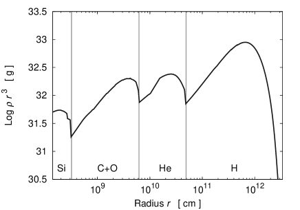
Figure 1.— $\rho\,r^{3}$ profile of the pre-supernova model. The composition interfaces of C+O/He and He/H are found at 6 $\times$ 10⁹ cm and 5 $\times$ 10¹⁰ cm, respectively. Regions of increasing $\rho\,r^{3}$ with increasing $r$ ($\rho\propto$ $r^{-\omega}$ with $\omega<3$) tend to be unstable against RT instability.

In Table 1, we summarize the models and the corresponding model parameters. The first column is the name of the model, the second is the parameter $\alpha$, the third is the $v_{\rm pol}/v_{\rm eq}$ corresponding to $\alpha$, the fourth is the $v_{\rm up}/v_{\rm down}$ (the definition will be described in §3.4), the fifth is the type of perturbations, the sixth is the amplitude of perturbations $\epsilon$, the seventh is the parameter $m$, and the eighth is the timing of perturbations. The fifth column, which is the type of perturbations, is either ‘random’, ‘sinusoidal’ or ‘clump’. ‘random’ and ‘sinusoidal’ denote that the forms of perturbations are $1+\epsilon\,(2\,{\rm rand}\,[m\,\theta/\pi]-1)$ and $1+\epsilon\sin(m\,\theta)$, respectively. ‘clump’ will be explained in §3.4. The seventh column, which is the timing of introducing the perturbations, is either ‘C+O/He’, ‘He/H’, ‘multi’, ‘shock’ or ‘full’. ‘C+O/He’ and ‘He/H’ mean that the perturbations are introduced when the shock wave reaches the composition interfaces of C+O/He and He/H, respectively. ‘multi’, ‘shock’, and ‘full’ will be explained in detail in §3.2, §3.4, and §3.5, respectively. The nomenclature for the names of models in the paper is as follows. The first character indicates whether the explosion is spherical (S) or aspherical (A), i.e., $\alpha=$ 0 or not. The second character is either ‘P’, ‘S’, ‘M’ or ‘T’. ‘P’ and ‘S’ mean ‘Pre-supernova’ and ‘Shock’ denoting the origins of the perturbations. ‘M’ means ‘Multiple’ whose perturbations are introduced in multiple times. ‘T’ means ‘Test’. Models with a second characters of ‘S’, ‘M’, and ‘T’ are described in later sections. If there are more than two models that have the same first two characters, a number is added to the name to distinguish the models. The models related to this particular section are SP1, SP2, and AP1 to AP8.

Table 1Models and parameters.

Model	$\alpha$	$v_{\rm eq}/v_{\rm pol}$	$v_{\rm up}/v_{\rm down}$	Type of perturb.	$\epsilon$	$m$	Timing of perturb.
SP1	0	1	1	random	5%	128	C+O/He
SP2	0	1	1	random	5%	128	He/H
SM	0	1	1	random	5%	128	multi
AP1	1/3	2	1	random	5%	128	C+O/He
AP2	3/5	4	1	random	5%	128	C+O/He
AP3	1/3	2	1	sinusoidal	5%	20	C+O/He
AP4	3/5	4	1	sinusoidal	5%	20	C+O/He
AP5	1/3	2	1	random	5%	128	He/H
AP6	3/5	4	1	random	5%	128	He/H
AP7	1/3	2	1	sinusoidal	5%	20	He/H
AP8	3/5	4	1	sinusoidal	5%	20	He/H
AT1	1/3	2	1	sinusoidal	30%	20	He/H
AT2	1/3	2	1	sinusoidal	30%	20	He/H
AS1	1/3	2	1	sinusoidal	30%	20	shock
AS2	1/3	2	2	clump	30%	3	shock
AS3	1/3	2	2	clump	30%	5	shock
AS4	1/3	2	2	clump	30%	7	shock
AS5	1/3	2	2	clump	30%	9	shock
AS6	1/3	2	2	clump	30%	11	shock
AS7	1/3	2	2	clump	30%	13	shock
AS8	1/3	2	2	clump	30%	15	shock
AM1	3/5	4	1	random	5%	128	multi
AM2	1/3	2	2	clump/random	30 / 5%	15 / 128	full
AM3	1/3	2	2	random	5%	128	multi

3.2. Aspherical explosions with multiply introduced perturbations of pre-supernova origins

In this section, we will explain models in which perturbations are introduced in multiple times. If the perturbations are introduced due to shell burning in the pre-collapse star, those could be multiply introduced. However, in the previous studies of RT mixing in supernovae, such situations have not been investigated. Therefore, we simply mimic perturbations multiply introduced in the pre-supernova star by introducing the perturbations in the radial velocities at different two times when the shock wave reaches the composition interfaces of C+O/He and He/H, respectively. Namely, the first perturbations are introduced when the shock wave reaches the composition interface of C+O/He and the second perturbations are introduced when the shock wave reaches the composition interface of He/H. We investigate models of both spherical and mildly aspherical explosions SM and AM1, respectively. The second character of the names of models in this section is ‘M’, which means ‘Multiple’ as explained above. In the two models, ‘random’ perturbations are employed. In table 1, the eighth column is represented by ‘multi’ for the models in this section.

3.3. Revisiting the best model in Nagataki et al.

Nagataki et al. (1998b) and Nagataki (2000) have investigated matter mixing in aspherical explosions using a pre-supernova mode for SN 1987A, and a mildly aspherical model of $v_{\rm pol}/v_{\rm eq}=$ 2 with sinusoidal perturbations of a large amplitude (30%) (model A1 in Nagataki et al.) have reproduced the high velocity of ⁵⁶Ni (up to $\sim$ 3,000 km s^-1). The pre-supernova model used in Nagataki et al. is the same as that in the present paper. Besides, the way of initiating the explosions is also basically same. However, the resolution of their simulations are rather low compared to that of recent studies of matter mixing in supernova explosions (e.g., Kifonidis et al., 2006) and the authors have not taken into account gravity, i.e., effects of fallback. Therefore, we revisit the best model in Nagataki et al. including the effects of gravity. We test two models AT1 and AT2, where the second character of the names ‘T’ means ‘Test’ as mentioned before. Model AT1 is the model whose setup of the simulation is basically the same as that of model A1 in Nagataki et al. In model AT1, effects of gravity is turned off, the total injected energy is set to be 10⁵¹ erg, the boundary condition of the radial inner edge is the ‘reflection’ boundary condition, $\alpha=$ 1/3 ($v_{\rm pol}/v_{\rm eq}=$ 2), $\epsilon=$ 30%, and the form of perturbations is ‘sinusoidal’ with $m=$ 20. Model AT2 is the counterpart of model AT1 whose model parameters are also the same as those of AT1 except that the effects of gravity are turned on and the boundary condition of the radial inner edge is switched to the ‘diode’ boundary condition at the later phase as in the other models in the present paper. In model AT2, the total injected energy is set to be 2 $\times$ 10⁵¹ erg because we have included gravitational potentials in this model. Note that the resultant explosion energy will be smaller than that of model AT1, if we inject the same 10⁵¹ erg as in model AT1. In both models, perturbations are introduced when the shock wave reaches the composition interface of He/H as in Nagataki et al. However, as the authors mentioned in their paper, such large perturbations with $\epsilon=$ 30% should be introduced in the supernova explosions itself. Therefore, we investigate the model AS1 whose model parameters and the setup of the simulation are the same as those of AT2 except for the timing of introducing the perturbations. In model AS1, the perturbations are introduced in the initial radial velocities as in the models described in the next section.

3.4. Aspherical explosions with clumpy structures

As mentioned in §1, theoretically, multi-dimensional effects are essential for a successful core-collapse supernova explosion. Recent multi-dimensional radiation hydrodynamic simulations of core-collapse supernova explosions have revealed that in the context of neutrino heating mechanisms, convection and SASI cause large anisotropy inside the standing shock and low-order unstable modes ($l$ = 1, 2) can grow dominantly (e.g., Marek & Janka, 2009; Suwa et al., 2010; Nordhaus et al., 2010; Takiwaki et al., 2012). Some models of neutrino-driven explosions aided by SASI have demonstrated that explosions may become stronger in either the north or south direction than those in the other directions across the equatorial plane (e.g., Marek & Janka, 2009; Suwa et al., 2010). Such asymmetry in explosions have thought to be the one of origins of neutron star kicks and proper motions of young pulsars (Scheck et al., 2006; Wongwathanarat et al., 2010). For example, we can see a globally anisotropic supernova shock wave whose morphology looks very clumpy (see e.g., Figure 1 in Hammer et al. (2010)). As mentioned in §1, Kifonidis et al. (2006) and Gawryszczak et al. (2010) have successfully reproduced high velocity clumps of ⁵⁶Ni in some models with neutrino-driven explosions. The authors have explained that the globally anisotropic explosion and the relatively large explosion energy (2 $\times$ 10⁵¹ erg) result in high velocity clumps of metals and strong RM instabilities at the composition interface of He/H. Such high velocity clumps can penetrate the dense helium core before the formation of a strong reverse shock. Strong RM instabilities at the interface of He/H cause a global anisotropy of the inner ejecta at late phases. However, their successful models remain small in number and the explosion energies involved are relatively large. Therefore, the conditions for reproducing the observed high velocity of ⁵⁶Ni are still not fully understood.

We explore matter mixing in such globally anisotropic explosions parametrically by mimicking the morphology of the explosion. We can see radially averaged physical values as a function of $\theta$ for an anisotropic explosion e.g., in Figure 11 in Gawryszczak et al. (2010). The distribution of radial velocity is relatively smooth but the distributions of density and velocity exhibit smaller-scale clumpy structures.

We mimic such globally anisotropic explosions as follows. First, we consider mildly aspherical explosion with $v_{\rm eq}/v_{\rm pol}$ = 2 ($\alpha$ = 1/3). Second, perturbations of a large amplitude (30%) with several smaller-scales are introduced in the initial radial velocities as

$$1+\sum^{4}_{n=1}\frac{\epsilon}{2^{(n-1)}}\sin(m\,n\,\theta),$$ (8)

where $\epsilon$ is the amplitude and $m$ is the integer parameter. We simply adopt the superposition of sinusoidal functions with different wave lengths and assume that the larger (smaller) the wavelength of the perturbations, the larger (smaller) the amplitude is. Third, we impose asymmetry across the equatorial plane by changing the normalizations of $v_{\rm r}$ across the equatorial plane as $v_{\rm up}/v_{\rm down}=$ 2, where $v_{\rm up}$ and $v_{\rm down}$ are the initial radial velocities at a radius inside the shock before imposing above perturbations (i.e., Equation (8)) at $\theta=$ 0^∘ and $\theta=$ 180^∘, respectively. The values of $v_{\rm up}/v_{\rm down}$ are shown in the fourth column of Table 1. We also test models having different base clump sizes (models AS2 to AS8) by changing the parameter $m$ ($m=$ 3 – 15). Figure 2 shows the distribution of the initial radial velocities at a radius inside the shock as a function of $\theta$ for model AS5. The second character of the names of models ‘S’ means ‘Shock’, which means that perturbations are imposed in the initial radial velocities. In Table 1, the eighth column is represented by ‘shock’ for the models described in this section.

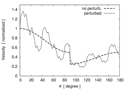
Figure 2.— Distribution of initial radial velocity at a radius inside the shock wave as a function of $\theta$ for model AS5. Radial velocities with perturbations given by Equation (8) (solid line) and those with no perturbation (dashed line) are shown. Values of the velocities are arbitrarily normalized.

3.5. Aspherical explosions with clumpy structures and multiply introduced perturbations of pre-supernova origins

Finally, we consider aspherical explosions with clumpy structures and multiply introduced perturbations of pre-supernova origins, i.e. multiple perturbations in a complete sense, which can be thought of as the combination of §3.2 and §3.4. For the perturbations introduced in the initial radial velocities, we adopt the perturbations given by Equation (8) ($\epsilon=$ 30% and $m=$ 15). For the perturbations of pre-supernova origins, ‘random’ perturbations ($\epsilon=$ 5% and $m=$ 128) are employed. We consider a globally aspherical explosion given by $v_{\rm pol}/v_{\rm eq}=$ 2 ($\alpha=$ 1/3) and $v_{\rm up}/v_{\rm down}=$ 2 as in models in §3.4. We refer to the model as AM2. The model parameters are listed in Table 1. The eighth column, the timing of the perturbations, is denoted by ‘full’. To see the impact of initial clumpy structures on the mixing, we add the model AM3 that have the same model parameters but with no perturbation in the initial radial velocities as a reference. Note that in the models in this sections AM2 and AM3, an energy of 2.5 $\times$ 10⁵¹ erg is injected to initiate the explosions.

4. Results

4.1. Spherical explosions with perturbations of pre-supernova origins

First, we will show the results from models of spherical explosions with perturbations of pre-supernova origins, i.e., models SP1, SP2, and SM. The density distributions in the $X$–$Z$ plane ($X=r\sin\theta$ and $Z=r\cos\theta$) at the ends of simulation time for models SP1, SP2, and SM are shown in Figure 3. We stop the calculation when the forward shock reaches close to the radius of 4.5 $\times$ 10¹² cm after the shock breakout. Models SP1 and SP2 are those in which random perturbations are introduced when the shock waves reach the composition interfaces of C+O/He and He/H, respectively. We can see the prominent RT fingers in both models above the radius of 1 $\times$10¹² cm. However, the lengths of the RT fingers are different between the two models. The lengths of RT fingers (hereafter the mixing lengths) in model SP1 is approximately 0.3 $\times$ 10¹² cm. On the contrary, the mixing length of model SP2 is roughly 0.6 $\times$ 10¹² cm. We find that in model SP1, perturbations grow around the composition interface of C+O/He due to RT instabilities but the fluctuations do not grow much after the shock wave has reached the composition interface of He/H. In model SP2, perturbations grow significantly around the composition interface of He/H. The morphology of RT fingers are also different between the two models. In model SP2, RT fingers are clearly distinguished. In model SP1, we can see prominent complex structures in the inner regions compared to model SP2. From above, the growth of RT instabilities around the composition interface of He/H is larger than that around the interface of C+O/He in our models. On the other hand, mixing of the inner regions is larger in model SP1 than that in model SP2.

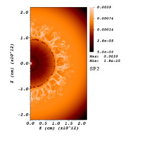
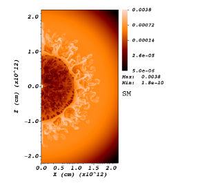
Figure 3.— Density distributions in the $X$–$Z$ plane at the ends of simulation time for models SP1 (left), SP2 (middle), and SM (right), which correspond to the time of 5986 s, 6006 s, and 5958 s, respectively. The unit of the values in the color bars is g cm^-3 and the values in the color bars are logarithmically scaled.

To find the cause of the differences seen between models SP1 and SP2, we perform a one-dimensional simulation of a spherical explosion with no perturbation. The total injected energy (2 $\times$ 10⁵¹ erg) and setups are the same as in other spherical models but now with no perturbation introduced. We estimate the growth factors of an initial seed perturbation using two growth rates as follows. One is the growth rate $\sigma$ for the incompressible fluid given by

$$\sigma=\sqrt{-\frac{P}{\rho}\mathscr{P}\,\mathscr{R}},$$ (9)

where $\mathscr{P}=\partial\ln P/\partial\,r$ and $\mathscr{R}=\partial\ln\rho/\partial\,r$. The other is the growth rate for the compressible fluid given by

$$\sigma=\frac{c_{s}}{\gamma}\sqrt{{\mathscr{P}}^{2}-\gamma\mathscr{P}\,\mathscr{R}},$$ (10)

where $c_{s}$ is the sound speed and $\gamma$ is the adiabatic index. The growth factor of an initial seed perturbation $\zeta/\zeta_{0}$ is given by

$$\frac{\zeta}{\zeta_{0}}=\exp\,\left(\int_{0}^{t}{\rm Re}\,[\,\sigma\,]\,\mathrm{d}t^{\prime}\right),$$ (11)

where $\zeta_{0}$ is the amplitude of the initial perturbation and $\zeta$ is the amplitude at the time of $t$ (see e.g., Müller et al. (1991)). The growth factors just after the shock breakout are shown in Figure 4. Overall, the growth factor for the compressible fluid is greater than that for the incompressible fluid. The growth factors are prominent around the composition interfaces of C+O/He and He/H. The growth factor around the interface of He/H is about one order-of-magnitude larger than that around the interface of C+O/He, which indicates that the growth of RT instabilities around the interface of He/H may be larger than that around the interface of C+O/He. We find that in model SP1, after the shock wave has passed through the interface, RT instabilities grow only around the interface of C+O/He and the forward shock propagates by roughly keeping a spherical symmetry. Therefore, in model SP1, when the shock wave reaches the interface of He/H, regions around the interface of He/H remain almost unperturbed and RT instabilities around the interface of He/H cannot grow well. While in model SP2, after the shock wave reaches the interface of He/H, RT instabilities start to grow. From the growth factors estimated above, the growth of RT instabilities around the interface of He/H may be larger than that around the interface of C+O/He, which is consistent with the results that the mixing lengths in model SP2 are larger than those in model SP1.

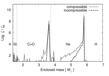
Figure 4.— Growth factors $\zeta/\zeta_{0}$ of an initial seed perturbation as a function of enclosed mass at the time of 5925 s. The total injected energy is 2 $\times$ 10⁵¹ erg as in other models. Two cases of growth factors are depicted. One is estimated by the growth rate for the incompressible fluid (solid line) and the other is estimated by that for the compressible fluid (dashed line). Overall, the growth factor for the compressible fluid is greater than that for the incompressible fluid. Growth factors are outstanding around the composition interfaces of C+O/He and He/H. Growth factor around the interface of He/H is about one order-of-magnitude greater than that around the interface of C+O/He.

In model SM, perturbations are introduced at different two times when the shock wave reaches the composition interfaces of C+O/H and He/H, respectively. Model SM has the features of both SP1 and SP2 (the right panel of Figure 3), i.e., the strong mixing of the inner regions and the prominent extension of RT fingers. The mixing length of model SM is nearly comparable to that of SP2 although more complex structures of RT fingers are observed. The structures of the inner regions are similar to that in model SP1. Note that somewhat more extended RT fingers are found around the polar region ($\theta\sim$ 0^∘) compared with those in other directions in model SP1 and SM, which may be responsible for discretization errors around the polar axis but the deviation from the basic spherical symmetry is not large.

The distributions of mass fractions for the elements ⁵⁶Ni, ²⁸Si, ¹⁶O, and ⁴He at the end of simulation time for model SM are shown in Figure 5. ⁵⁶Ni is concentrated inside the dense helium shell around the radius of 1 $\times$ 10¹² cm. ²⁸Si encompasses the inner ⁵⁶Ni and a small fraction of ²⁸Si is conveyed outward along the RT fingers. ¹⁶O is prominent at the bottom of the helium shell and inside the RT fingers. ⁴He is found to be the most abundant around the RT fingers. ⁴He are also seen inside the helium shell, which is responsible for the explosive nucleosynthesis.

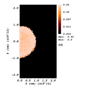
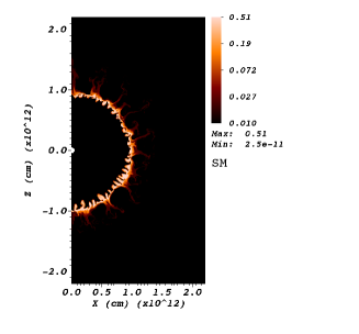
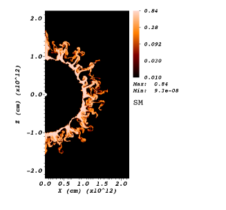
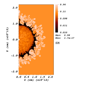
Figure 5.— Distributions of mass fractions of elements ⁵⁶Ni (top left), ²⁸Si (top right), ¹⁶O (bottom left), and ⁴He (bottom right) at the end of simulation time in the $X$–$Z$ plane for model SM, which corresponds to the time of 5958 s. Values in the color bars are logarithmically scaled and the minimum value in the color bars is set to be 1 $\times$ 10^-2.

The mass distributions of elements ¹H, ⁴He, ¹²C, ¹⁶O, ²⁸Si, ⁴⁴Ti, and ⁵⁶Ni as a function of radial velocity at the ends of simulation time for models SP1, SP2, and SM are shown in Figure 6. In model SP2, we can see slight enhancements of the high velocity component of ¹²C, ¹⁶O, and ²⁸Si around 2,000 km s^-1 and a low velocity tail of ¹H compared with those of model SP1. On the other hand, in model SP1, enhancements of low-velocity tails of the inner most metals ⁵⁶Ni and ⁴⁴Ti are seen. RT instabilities grown around the composition interface of He/H mix up elements of ¹H, ⁴He, ¹²C, ¹⁶O, and ²⁸Si more efficiently than that around the interfaces of C+O/He. While, RT instabilities developed around the interface of C+O/He convey the innermost metals farther outward than that around the interface of He/H. Same as Figure 3, model SM has the features of both SP1 and SP2, i.e., enhancements of high velocity components of ¹²C, ¹⁶O, and ²⁸Si and a low-velocity tail of ¹H compared to SP1, as well as enhancements of low-velocity tails of ⁵⁶Ni and ⁴⁴Ti. In all three models, the distributions of ⁴⁴Ti are quite similar to those of ⁵⁶Ni. The obtained maximum radial velocity of ⁵⁶Ni is approximately 1,600 km s^-1 and the minimum radial velocity of ¹H is 800 km s^-1 among the three models, where we define the maximum (minimum) radial velocity as that among the bins with $\Delta M_{i}/M_{i}>1\times$ 10^-3.

For reference, we also perform a simulation of a spherical explosion without any imposed perturbation. The setup and the initial conditions are same as in models SP1, SP2, and SM but for no imposed perturbation. We recognize a growth of some perturbations in this reference model. At the end of the simulation time, radial folds above the reverse shock and slight rippled structures around the forward shock in density are seen. We find with a touch of surprise that the maximum velocity of ⁵⁶Ni (1,700 km s^-1) is larger than those of any other spherical explosion models in this section, i.e., SP1, SP2, and SM. However, the growth of RT instability around the composition interface of He/H are rather small and the mixing of ¹H into inner cores is negligible. The obtained minimum velocity of ¹H is 1,700 km s^-1 and which is the largest among spherical explosion models. The perturbations may be introduced by grids and/or remappings and the wavelengths of the perturbations could be smaller than those of the imposed perturbations in the models in the paper. Since the growth of the perturbation with a smaller wavelength is faster than that of the perturbation with a larger wavelength, the introduced perturbations can grow even in a small dynamical time scale in a relatively early phase.

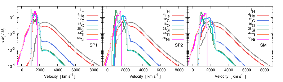
Figure 6.— Mass distributions of elements, ¹H, ⁴He, ¹²C, ¹⁶O, ²⁸Si, ⁴⁴Ti, and ⁵⁶Ni, as a function of radial velocity at the ends of simulation time for models SP1 (left), SP2 (middle), and SM (right), which correspond to the time of 5986 s, 6006 s, and 5958 s, respectively. $\Delta M_{i}$ is the mass of the element with index $i$ in the velocity range of $v\sim v+\Delta v$. $M_{i}$ is the total mass of the element with index $i$. For the binning of radial velocity, $\Delta v=$ 100 km s^-1 is adopted.

In Table 2, we summarize the results of our models. The first column is the explosion energy, $E_{\rm exp}$, at the end of simulation time, the second column is the obtained minimum radial velocity of hydrogen $v_{r,{\rm min}}$ (¹H) and the third column is the obtained maximum radial velocity of ⁵⁶Ni $v_{r,{\rm max}}$ (⁵⁶Ni). The explosion energy $E_{\rm exp}$ is estimated as

$$E_{\rm exp}=2\pi\int_{r_{1}}^{r_{2}}\int_{0}^{\pi}\left(\frac{1}{2}\,\rho\,\mbox{\boldmath$v$}^{2}+\rho\,E+\rho\,\Phi\right)r^{2}\sin\theta\,\mathrm{d}r\,\mathrm{d}\theta,$$ (12)

where $r_{1}$ ($r_{2}$) is the radius of the inner (outer) edge of the computational domain, $\Phi$ is the gravitational potential and the integrand is summed up only when it is positive. In models SP1, SP2, and SM, the obtained explosion energies are approximately 1.4 $\times$ 10⁵¹ erg at the ends of simulation time. The maximum velocities of ⁵⁶Ni are approximately 1,500 km s^-1, which is much smaller than the observed values of SN 1987A ($\sim$ 4,000 km s^-1) as mentioned above. In models SP2 and SM, the minimum velocity of ¹H is 800 km s^-1, which is consistent with the theoretically inferred values (Shigeyama & Nomoto, 1990; Kozma & Fransson, 1998). Therefore, inward mixing of hydrogen may be caused by the RT instability around not the interface of C+O/He but the interface of He/H.

Table 2Results of models.

Model	$E_{\rm exp}$	$v_{r,{\rm min}}$(1H)	$v_{r,{\rm max}}$(56Ni)
	(erg)	(km s-1)	(km s-1)
SP1	1.43 (51)	1,400	1,600
SP2	1.43 (51)	900	1,500
SM	1.44 (51)	800	1,500
AP1	1.48 (51)	1,300	1,600
AP2	1.50 (51)	1,100	1,600
AP3	1.47 (51)	1,300	1,600
AP4	1.50 (51)	1,000	1,600
AP5	1.48 (51)	900	1,500
AP6	1.51 (51)	900	1,500
AP7	1.47 (51)	800	1,300
AP8	1.50 (51)	800	1,200
AM1	1.51 (51)	700	1,700
AT1	–	500	3,300
AT2	1.51 (51)	600	3,100
AS1	1.54 (51)	1,500	1,900
AS2	1.28 (51)	900	1,900
AS3	1.50 (51)	1,200	2,200
AS4	1.51 (51)	1,300	2,100
AS5	1.51 (51)	1,300	1,800
AS6	1.51 (51)	1,200	1,900
AS7	1.52 (51)	1,200	1,800
AS8	1.51 (51)	1,200	1,900
AM2	2.03 (51)	1,100	3,000
AM3	1.99 (51)	1,100	2,100

4.2. Aspherical explosions with perturbations of pre-supernova origins

In this section, we present our results for models of aspherical explosions with perturbations of pre-collapse origins, i.e., models AP1 to AP8 and AM1. The density distributions for models AP1, AP2, AP3, and AP4 are shown in Figure 7. In models AP1 to AP4, perturbations are introduced when the shock waves reach the interface of C+O/He. In models AP1 and AP2, ‘random’ perturbations are introduced but the degree of asphericity ($v_{\rm pol}$/$v_{\rm eq}$) are different. More extended RT fingers produced by model AP2 are seen around the polar regions than those produced by model AP1. In models AP3 and AP4, the situation is similar to that in models AP1 and AP2 but the perturbations are sinusoidally introduced. The mixing lengths in models AP3 and AP4 are comparable with those in models AP1 and AP2, respectively. Compared to RT fingers produced by models AP1 and AP3, those produced by more aspherical explosion models AP2 and AP4 have smaller-scale. In model AP3 and AP4, prominent protrusions along the polar axis are given. Compared with the spherical explosion cases, in aspherical models, AP1 to AP2, the shapes of the dense shells around the radius of 1 $\times$ 10¹² cm deviate slightly from the spherical symmetry and the corresponding positions are shifted inward in the regions closer to the polar axis.

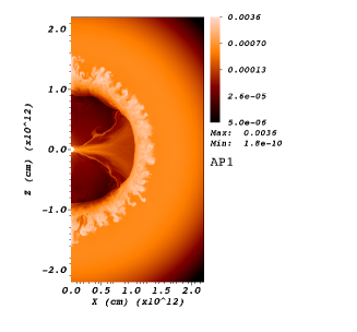
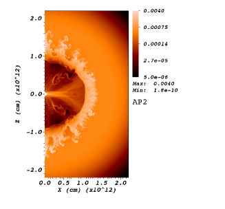
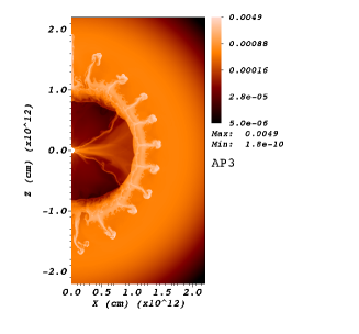
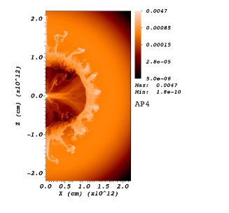
Figure 7.— Same as Figure 3 but for models AP1 (top left), AP2 (top right), AP3 (bottom left), and AP4 (bottom right) and the time of 5851 s, 5773 s, 5861 s, and 5781 s, respectively.

The density distributions for models AP5, AP6, AP7, and AP8 are shown in Figure 8. In models AP5 to AP8, perturbations are introduced when the shock waves reach the interface of He/H. In overall, the mixing lengths in models AP5 to AP8 are apparently enhanced compared to those in models AP1 to AP4. We further recognize enhanced inward mixing in regions close to the polar axis in models AP5 to AP8 compared with those in models AP1 to AP4 from the positions of the inner edges of the dense shells. The mixing lengths derived from ‘sinusoidal’ perturbation models AP7 and AP8 are enlarged compared with those in the counterparts of ‘random’ perturbation models AP5 and AP6, respectively. The RT fingers in model AP8 have stronger wobbling than those in model AP7, because model AP8 has clearer aspherical feature than model AP7.

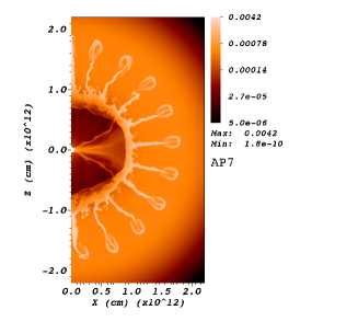
Figure 8.— Same as Figure 3 but for models AP5 (top left), AP6 (top right), AP7 (bottom left), and AP48 (bottom right) and the time of 5859 s, 5781 s, 5881 s, and 5793 s, respectively.

The mass distributions of elements as a function of radial velocity at the ends of simulation time for models AP1, AP2, AP3, and AP4 are shown in Figure 9. The high velocity tails of ⁵⁶Ni, ²⁸Si, ¹²C, and ¹⁶O in model AP2 are slightly enhanced compared with those in model AP1, because AP2 has clearer aspherical feature than model AP1. As summarized in Table 2, the obtained maximum velocity of ⁵⁶Ni are approximately 1,600 km s^-1 in models AP1 and AP2. The low-velocity tail of hydrogen is slightly more prominent in model AP1 compared to that in model AP2. In models AP3 and AP4, the obtained maximum velocity of ⁵⁶Ni are comparable to those in models AP1 and AP2. However, the high velocity components of ²⁸Si, ¹²C, and ¹⁶O in sinusoidal perturbation models AP3 and AP4 are enhanced compared with those in the random perturbation models AP1 and AP2. The minimum velocities of ¹H range between 1,000 and 1,300 km s^-1 among models AP1 to AP4. The inward mixing in models AP2 and AP4 is more prominent than that in models AP1 and AP3. The minimum velocities of ¹H in models AP2 and AP4 are smaller than those in models AP1 and AP3. The reason is because models AP2 and AP4 have clearer aspherical feature than models AP1 and AP3.

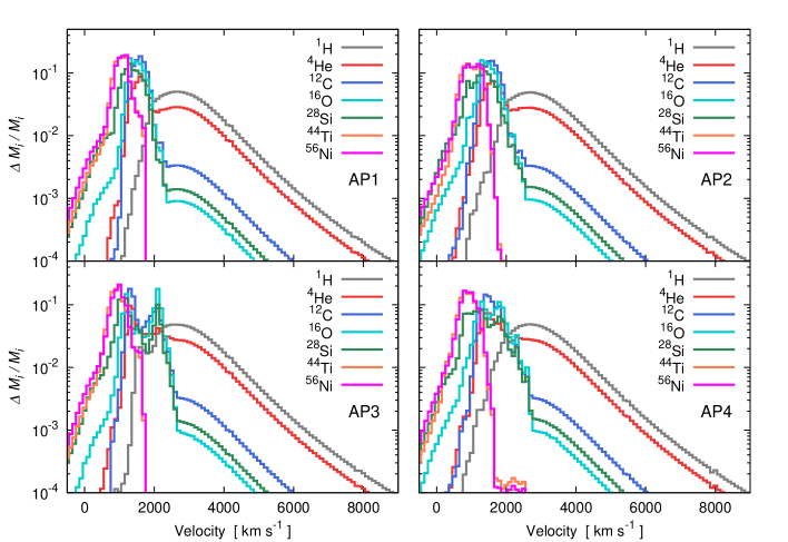
Figure 9.— Same as Figure 6 but for models AP1 (top left), AP2 (top right), AP3 (bottom left), and AP4 (bottom right) and the time of 5851 s, 5773 s, 5861 s, and 5781 s, respectively.

The mass distributions of elements, ¹H, ⁴He, ¹²C, ¹⁶O, ²⁸Si, ⁴⁴Ti, and ⁵⁶Ni, as a function of radial velocity at the ends of simulation time for models AP5, AP6, AP7, and AP8 are shown in Figure 10. In models AP5 to AP8, perturbations are introduced when shock waves reach the interface of He/H. Overall, high velocity tails of ²⁸Si, ¹²C, and ¹⁶O in models AP5 to AP8 are enlarged compared with those in models AP1 to AP4, because models AP5 to AP8 have prominent RT instabilities around the composition interface of He/H. However, the maximum velocities of inner most metals such as ⁵⁶Ni and ⁴⁴Ti are reduced in models AP5 to AP8 compared with those in models AP1 to AP4. Obtained maximum velocities of ⁵⁶Ni range between 1,200 and 1,500 km s^-1 among models AP5 to AP8. On the other hand, the minimum velocities of ¹H are smaller than those in models AP1 to AP4 and range between 800 and 900 km s^-1. From above results, mixing of innermost metals, ⁵⁶Ni and ⁴⁴Ti is prominent in models that perturbations are introduced in an early phase. On the contrary, mixing of the other elements is prominent in models where perturbations are introduced in a later phase. Overall, the mixing is slightly enhanced in models with strong aspherical feature compared with models with weaker aspherical feature. In all aspherical explosion modes AP1 to AP8, the obtained maximum velocities of ⁵⁶Ni do not reach the observed high values of SN 1987A.

Figure 10.— Same as Figure 6 but for models AP5 (top left), AP6 (top right), AP7 (bottom left), and AP8 (bottom right) and the time of 5859 s, 5781 s, 5881 s, and 5793 s, respectively.

Next, we show the results of the aspherical explosion model AM1 in which perturbations are multiply introduced. First, we explain briefly the explosive nucleosynthesis by taking model AM1 as an example. The distributions of mass fractions of elements, ⁵⁶Ni, ²⁸Si, ⁴He, and ⁴⁴Ti, are shown as the results at the evolutionary time of 0.96 s for model AM1 in Figure 11. The values in color bars are linearly scaled. ⁵⁶Ni is synthesized prominently in the edge of a gourd-like structure and inner regions close to the polar axis (the top left panel). In the thin edge of the gourd-like structure, ²⁸Si remains unburned partly due to the incomplete silicon burning. Inside the gourd-like structure, some fraction of ⁴He also remains unburned. The regions that ⁴He remains unburned correspond to relatively low density regions inside the shock. In a low density regime, the explosive silicon burning ends up with so-called the alpha-rich freeze-out. ⁴⁴Ti is prominent in regions that ⁴He remains unburned due to the alpha-rich freeze-out. This is consistent with the results of Nagataki (2000).

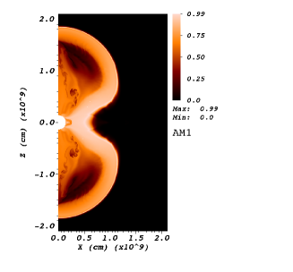
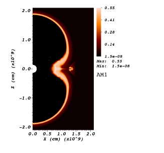
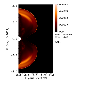
Figure 11.— Distributions of mass fractions of elements, ⁵⁶Ni (top left), ²⁸Si (top right), ⁴He (bottom left), and ⁴⁴Ti (bottom right) at the time of 0.96 s in the $X$–$Z$ plane for model AM1. The values in color bars are linearly scaled.

We show the time evolution of density distribution for model AM1. The snap shots of density distributions for model AM1 at the time of 0.53 s, 16.6 s, 288 s, and 5752 s are shown in Figure 12. Note that the white color regions are outside of the computational domain. A gourd-shaped shock is generated by the bipolar explosion as shown in the top left panel just after the initiation of the explosion. The snap shot just after the introduction of the first perturbations is shown in the top right panel. We recognize that the gourd-shaped shock becomes narrower in equatorial regions due to the fallback of matter. The snap shot after the introduction of the second perturbations is shown in the bottom left panel. Finally, the snap shot at the end of simulation time is shown in the bottom right panel. The appearance of the density distribution is similar to that in model AP6 (see the top left panel in Figure 8). However, more prominent inward and outward mixing is seen around the polar regions. The mixing length around the polar region is approximately 1 $\times$ 10¹² cm. We can more extended RT fingers along the polar axis, which reach the radius of 2 $\times$ 10¹² cm.

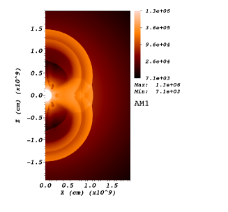
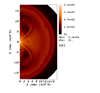
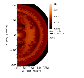
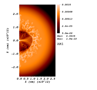
Figure 12.— Snap shots of distributions of density at the time of 0.53 s (top left), 16.6 s (top right), 288 s (bottom left), and 5752 s (bottom right) for model AM1. The unit of values in color bars is g cm^-3. The values in color bars are logarithmically scaled.

The distributions of mass fractions of elements, ⁵⁶Ni, ²⁸Si, ¹⁶O, and ⁴He, for model AM1 at the end of simulation time are shown in Figure 13. Unlike the results in spherical explosion models shown in Figure 5, here ⁵⁶Ni is distributed in the wedge-shaped regions around the polar axis. Slight protrusions of ⁵⁶Ni along the RT fingers are also seen. However, ⁵⁶Ni is basically concentrated inside the dense helium shell. ²⁸Si encompasses ⁵⁶Ni. Some fractions of ²⁸Si are conveyed outward along the RT fingers. ¹⁶O is prominent in a wedged-shaped region along the equatorial plane and inside the RT fingers. ⁴He is distributed around the RT fingers and the inner wedge-shaped regions along the polar axis. ⁴He in inner regions are synthesized by the explosive nucleosynthesis, as same as the process in the spherical explosion models.

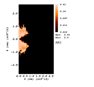
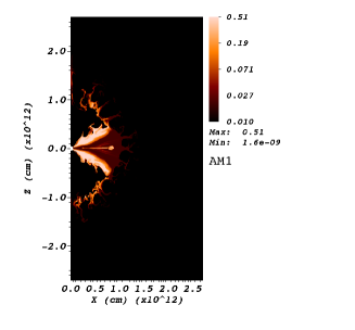
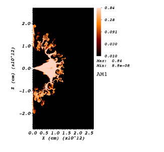
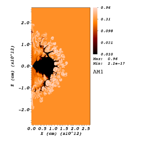
Figure 13.— Same as Figure 5 but for elements, ⁵⁶Ni, ²⁸Si, ¹⁶O, and ⁴He and the time of 5752 s.

In Figure 14, we show the mass distributions of elements, ¹H, ⁴He, ¹²C, ¹⁶O, ²⁸Si, ⁴⁴Ti, and ⁵⁶Ni, as a function of radial velocity for model AM1 at the end of simulation time. As expected from the previous discussion, the distributions have features seen in both models of AP2 and AP6. The high velocity tails of ²⁸Si, ¹²C, and ¹⁶O in model AM1 are enhanced compared with those in model AP2. The innermost metals, ⁵⁶Ni and ⁴⁴Ti, in model AM1 are conveyed in higher velocity regions compared with the situation in model AP6. The maximum velocity of ⁵⁶Ni reaches 1,700 km s^-1, which is the largest value among all the models mentioned above.

The mass distributions of ⁵⁶Ni as a function of line of sight velocity at the end of simulation time for model AM1 are shown in Figure 15. The mass distributions of three observer angles $\theta_{\rm ob}$ = 90^∘, 135^∘, and 180^∘ are given. Note that the vertical values are linearly scaled and the shapes of the mass distributions approximately correspond to the observable line profiles of [Fe II]. Appearances of mass distributions are rather different by the observer angles as expected. If $\theta_{\rm ob}=$ 90^∘, the distribution is well symmetric across the null velocity point. and the distribution concentrates around the point. If the observer angle is 180^∘ and the bipolar explosion is seen head on, the distribution prominently split into the red-shifted and blue-sifted sides. The peaks locate around the line of sight velocities of $\pm$ 1,000 km s^-1. In the case of $\theta_{\rm ob}=$ 135^∘, the split distribution is relatively moderate but we can recognize distinct double peaks. Note that other aspherical explosion models AP1 to AP8 have basically same features. Even if the head-on explosion is seen by an observer, the tails are extended only up to values of $\pm$ 1,500 km s^-1. As stated in §1, the observed line profile of [Fe II] in SN 1987A is asymmetric across the peak of the flux distribution (Haas et al., 1990). Therefore, the morphology of the explosion of SN 1987A may not be a simple bipolar explosion symmetric across the equatorial plane.

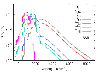
Figure 14.— Same as Figure 6 but for model AM1 at the time of 5752 s.

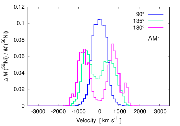
Figure 15.— Mass distributions of ⁵⁶Ni as a function of line of sight velocity at the end of simulation time (5752 s) for model AM1. The mass distributions of three observer angles $\theta_{\rm ob}$ = 90^∘, 135^∘, and 180^∘ are shown. $\Delta M$ (⁵⁶Ni) is the mass of ⁵⁶Ni in the velocity range of $v\sim v+\Delta v$. $M$ (⁵⁶Ni) is the total mass of ⁵⁶Ni. For binning of line of sight velocity, $\Delta v=$ 100 km s^-1 is adopted.

4.3. Results of revisiting the best model in Nagataki et al.

This section is devoted to present the results of model AT1, AT2, and AS1. The summary of the results of model AT1 is shown in Figure 16. We can see marked RT fingers in the density distribution shown in the top left panel. ⁵⁶Ni is distributed inside both the dense shell around the radius of 0.7 $\times$ 10¹² cm and inner regions of RT fingers. The number of RT fingers are consistent with the wave lengths of imposed perturbations, i.e., the parameter $m$. Strong mixing of metals ⁵⁶Ni, ⁴⁴Ti, ²⁸Si, ¹⁶O, and ¹²C is seen in the bottom left panel of Figure 16. The obtained maximum velocity of ⁵⁶Ni with $\Delta M$ (⁵⁶Ni)/$M$ (⁵⁶Ni) $>$ 1 $\times$ 10^-3 is 3,300 km s^-1 (see Table 2), which is roughly consistent with that in Nagataki (2000). A small fraction of ⁵⁶Ni with $\Delta M$ (⁵⁶Ni)/$M$ (⁵⁶Ni) $>$ 1 $\times$ 10^-4 reaches velocity of 3,500 km s^-1. Strong inward mixing of ¹H is also seen. The obtained minimum velocity of ¹H is 500 km s^-1. The mass distributions of ⁵⁶Ni as a function of line of sight velocity are depicted in the bottom right panel of Figure 16. For all observer angles, the tails of mass distributions are extended around $\pm$ 3,000 km s^-1. Sharp decays of the distributions across $\pm$ 1,000 km s^-1 are seen. These are somewhat different from the observed smooth flux distributions of [Fe II] in SN 1987A. The sharp decays of the distributions is also somewhat different from the distribution seen in model A1 in Nagataki et al. (see e.g., Fig. 14 in Nagataki (2000)) wherein the smoother decay than those of model AT1 are seen. The differences may be attributed to the different hydrodynamic code used and the different resolutions of simulations.

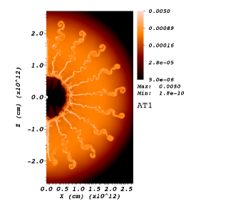
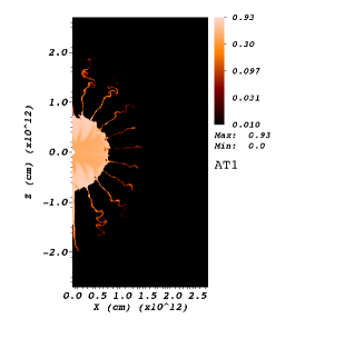
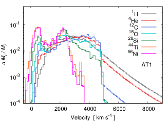
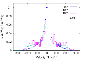
Figure 16.— Results of model AT1 at the time of 5060 s, the density distribution (top left), the distribution of the mass fraction of ⁵⁶Ni (top right), the mass distributions of elements as a function of radial velocity (bottom left), and the mass distributions of ⁵⁶Ni as a function of the line of sight velocity (bottom right).

The summary of the model AT2 results is shown in Figure 17. The ‘diode’ boundary condition is employed for the inner radial boundary in later phases and gravity is turned on as noted in §3.3. The appearance of RT fingers is quite similar to that of model AT1 (the top left panel). However, the density distribution of inner regions is different from that of model AT1 due to the effects of fallback. The distribution of ⁵⁶Ni is also different from that of model AT1. ⁵⁶Ni is distributed only in regions apart from the equatorial plane. The mass distributions of elements as a function of radial velocity are shown in the bottom left panel of Figure 17. These mass distributions are similar to those of model AT1. The obtained maximum velocity of ⁵⁶Ni is 3,100 km s^-1, which is somewhat reduced compared with that of model AT1 (see Table 2). The minimum velocity of ¹H (600 km s^-1) is similar to that of model AT1. From the bottom right panel of Figure 17, we see that the distributions of ⁵⁶Ni as a function of line of sight velocity are clustered around the null velocity point compared with those in model AT1. From above results, even if the effects of fallback are included in the simulation, the high velocity of ⁵⁶Ni can be reproduced by model AT2. However, as Nagataki (2000) stated, such large perturbations (amplitude of 30%) might not be introduced in the pre-collapse star. Hence, we calculate the model AS1 that has same setups and model parameters as model AT2 but perturbations (amplitude of 30%) are introduced in the initial radial velocities. Hereafter, we show the results of model AS1.

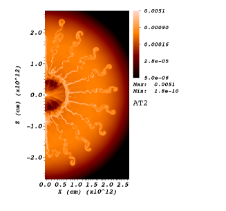
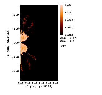
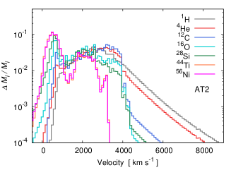
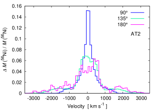
Figure 17.— Same as Figure 16 but for model AT2 and the time of 5567 s.

In Figure 18, we show the time evolution of density distribution of model AS1. Just after the initiation of the explosion (1.36 s after the explosion), outward finger structures, which is attributed to the imposed large perturbations, are clearly seen (the top left panel). We can also recognize inward finger structures adjacent to outward ones. The inward mixing may be caused by RT instabilities due to the inward gravitational force. However, after that, the finger structures are gradually broken up due to KH instability (the top right panel). Along the polar axis, relatively large-sale protrusions of inner matter are seen. This occurs physically because the explosion along the polar regions is the strongest, but this may be partly affected by numerical errors around the polar axis. After the formation of the dense helium shell, the fingers are almost destroyed due to the collision with the dense shell (the bottom left panel). Eventually, no protrusion of innermost metals is seen except for polar regions (the bottom right panel). The mass distributions of elements as a function of radial velocity are shown in Figure 19. All metals ⁵⁶Ni, ⁴⁴Ti, ²⁸Si, ¹²C, and ¹⁶O are limited at the velocity around 2,000 km s^-1, which corresponds to around the bottom of the dense helium shell. A part of innermost metals ⁵⁶Ni and ⁴⁴Ti can reach the dense shell but cannot penetrate the shell. The mass distributions of ⁵⁶Ni as a function of line of sight velocity are shown in Figure 20. In all observer angles, a clear cut off of velocity around $\pm$ 1,500 km s^-1 is seen. The maximum radial velocity of ⁵⁶Ni is 1,900 km s^-1 and the minimum radial velocity of ¹H is 1,500 km s^-1. A strong inward mixing of ¹H does not occur in this model.

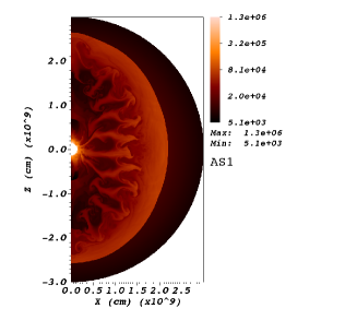
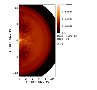
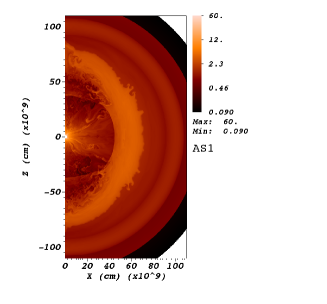
Figure 18.— Snap shots of distributions of density at the time of 1.36 s (top left), 8.57 s (top right), 147.4 s (bottom left), and 5753 s (bottom right) for model AS1. The unit of values in color bars is g cm^-3. The values in color bars are logarithmically scaled.

From the results in this section, we summarize as follows. The high velocity of ⁵⁶Ni seen in models AT1 and AT2 cannot be reproduced if the same perturbations are imposed in the initial radial velocities. The initial perturbations cannot retain the structures in later phases in which RT instability around the composition interface of He/H grows. In other wards, if such structures remain and/or exist due to some unknown reasons, such high velocity of ⁵⁶Ni might be reproduced. In the next section, we focus on the models in which large perturbations are introduced in initial radial velocities.

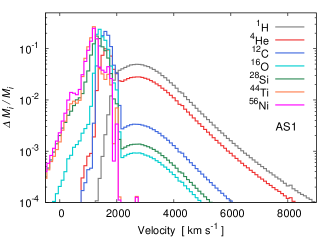
Figure 19.— Same as Figure 6 but for model AS1 at the time of 5753 s.

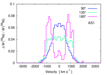
Figure 20.— Same as Figure 15 but for model AS1 and the time of 5753 s

4.4. Aspherical explosions with clumpy structures

In this section, we show the results of aspherical explosion models with clumpy structures. In the previous sections, we consider bipolar explosions. In this section, explosions are also asymmetric across the equatorial plane, i.e, $v_{\rm up}/v_{\rm down}$ = 2 (see Table 1). In models AS2 to AS8, we change the size of clumpy structure in the initial shock waves by setting different parameter $m$ in Equation (8). The density distributions at the ends of simulation time for models AS2, AS3, AS5, and AS8 as representative models are shown in Figure 21. In all models AS2 to AS8, small-scale RT fingers are developed around the bottom of the dense helium shell and RT fingers in the upper hemisphere are slightly longer than those in the lower one. For models AS2 to AS5, the configurations of the fingers are different from each other in the upper hemisphere. While, for models that have smaller-scale clumps, i.e., AS6 to AS8, the differences of the configurations of fingers are not distinctive. In models AS3 and AS5, prominent extended fingers are seen very close to the polar axis. This is a common problem seen in a two-dimensional axisymmetric hydrodynamic simulation. This problem is partly attributed to the effects that flows cannot penetrate across the symmetry axis and discretization errors around the axis. However, it reflects the physical nature that the explosion is strongest in regions close to the polar axis. Unfortunately, we hardly speculate how the features are realistic in a two-dimensional axisymmetric calculation. Figure 22 depicts the mass distributions of elements as a function of radial velocity at the ends of simulation time for models AS2, AS3, AS5, and AS8. For models of relatively larger-scale clumps, AS2 to AS5, the maximum velocity of innermost metals ⁵⁶Ni and ⁴⁴Ti are affected by the sizes of clumpy structures. In model AS3, the high velocity tails of ⁵⁶Ni and ⁴⁴Ti are smoothly extended around 3,000 km s^-1 and a small amount of high velocity clumps (up to 4,000 km s^-1) is recognized. Model AS5 has also a slightly extended high velocity wing and a small amount of high velocity ⁵⁶Ni clump. On the other hand, in models AS6 to AS8, the mass distributions are similar to each other and the maximum velocity of innermost metals are limited to around 2,000 km s^-1. From above results, we know that the size of clump may affect the protrusion of innermost metals and the clump with a relatively larger size tend to penetrate the dense helium shell more easily. However, it is difficult to find a monotonic behavior with respect to the penetration of innermost metals. The results are somewhat sensitive to the clump size. Additionally, we find that the high velocity clumps of ⁵⁶Ni is clustered only in regions very close to the polar axis. Therefore, the high velocity clumps of ⁵⁶Ni seen in models AS3 and AS5 are doubtful. It is noted that strong RM instabilities around the composition interface of He/H obtained by Kifonidis et al. (2006) (see §1 and §3.4) are not confirmed in models AS2 to AS8. In fact, as summarized in Table 2, the minimum radial velocities of ¹H range between 1,200 to 1,300 km s^-1 except for that for model AS2 (that is about 900 km s^-1). Therefore, strong inward mixing of ¹H due to RM instabilities is not realized in models AS2 to AS8. The differences may be due to the following facts: the progenitor model, a 15 $M_{\odot}$ blue supergiant star (see Figure 8 in Kifonidis et al. (2003)), is different from ours and our models do not duplicate some features of a neutrino-driven explosion model, such as initial angular velocities and their gradients, thermal and density structures, and so on.

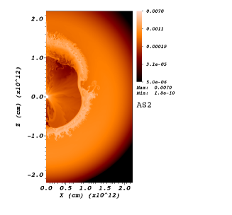
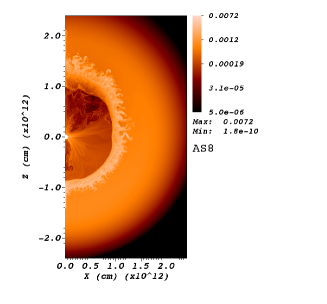
Figure 21.— Same as Figure 3 but for models AS2 (top left), AS3 (top right), AS5 (bottom left), and AS8 (bottom right) and at the time of 5548 s, 5250 s, 5225 s, and 5231 s, respectively.

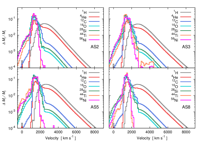
Figure 22.— Same as Figure 6 but for models AS2 (top left), AS3 (top right), AS5 (bottom left), AS8 (bottom right) and at the time of 5548 s, 5250 s, 5225 s, and 5231 s, respectively.

In the previous models in the paper, no high velocity of ⁵⁶Ni ($\gtrsim$ 3,000 km s^-1) is obtained except the cases in the test models AT1 and AT2. Therefore, we finally consider the perturbations of both initial shock waves and pre-supernova origins, i.e., model AM2. The time evolution of the density distribution for model AM2 is shown in Figure 23. After the initiation of the explosion, a globally anisotropic shock wave asymmetric across the equatorial plane propagates outward (the top left panel). Inside the shock wave, smaller-sale clumpy structures, i.e., outward and inward fingers, are also seen. After the shock wave passes through the composition interface of C+O/He, perturbations grow due to RT instabilities around the composition interface (the top right panel). At this phase, first moving clumps of ⁵⁶Ni reach the interface and are conveyed outward with the aid of RT instabilities. Then, RT instabilities around the composition interface of He/H are developed (the bottom left panel). We find that the multiply introduced perturbations make some fractions of innermost metals including ⁵⁶Ni reach around the bottom of the dense helium shell and penetrate it. Eventually, prominent RT fingers are developed in particular in the upper hemisphere (the bottom right panel).

The distributions of mass fractions of elements ⁵⁶Ni, ²⁸Si, ¹⁶O, and ⁴He are shown in Figure 24. We can see that most of ⁵⁶Ni is confined inside the dense helium shell. However, some fraction of ⁵⁶Ni penetrates the shell along RT fingers (the top left panel). We emphasize that the penetrations of ⁵⁶Ni are seen not only in regions close to the polar axis but also in regions away from the polar axis. ²⁸Si is prominent around the ⁵⁶Ni (the top left panel). ¹⁶O is outstanding in regions inside the dense helium shell in the lower hemisphere and in RT fingers (the bottom left panel). ⁴He is mixed inward due to RT instabilities (the bottom right panel). It should be noted that the obtained morphology of inner ejecta such as ⁵⁶Ni, ²⁸Si, and ¹⁶O, is roughly elliptical and the ratio of the major to minor axes is approximately 2. These are roughly consistent with the recent observation of supernova remnant SN 1987A (1.8 $\pm$ 0.17: Kjær et al., 2010).

The mass distributions of elements at the end of simulation time as a function of radial velocity for model AM2 are shown in Figure 25. The largest value of the velocity of ⁵⁶Ni clump achieves around 3,000 km s^-1. We find that the amount of ⁵⁶Ni with velocity over 2,700 km s^-1 is approximately 1.4 $\times$ 10^-3 $M_{\odot}$. The high velocity tails of other metals, ²⁸Si, ¹²C, and ¹⁶O, are also enhanced compared with those in models AS2 to AS8. Note that models AS2 to AS8 have no perturbation of pre-supernova origins (see Figure 22). The minimum velocity of ¹H (1,100 km s^-1, see Table 2) is slightly smaller than that of models AS2 to AS8 (1,200 – 1,300 km s^-1). This indicates inward mixing of ¹H is slightly enhanced compared with models AS2 to AS8. But strong inward mixing of ¹H seen in e.g., models AM1 and AT2 is not realized in model AM2. The possible reason are that the higher explosion energy ($\sim$ 2 $\times$ 10⁵¹ erg) minifies the time for RT instabilities to grow and a globally aspherical explosion makes the amount of inward ¹H to be small.

To see the effects of clumpy structures, we perform the model AM3 which has no clumpy structure given by Equation (8) as a counterpart of model AM2. The mass distributions of elements as a function of radial velocity are shown in Figure 26. We can see very small fraction of ⁵⁶Ni is clustered around 3,000 km s^-1. But the fraction is rather smaller than that of model AM2. This means that initial clumpy structures are important for ⁵⁶Ni to be conveyed into high velocity regions.

The mass distributions of ⁵⁶Ni as a function of line of sight velocity are shown in Figure 27. If $\theta_{\rm ob}=$ 90^∘, the distribution is clustered around the null velocity point and the high velocity tails reach around $\pm$ 1,500 km s^-1. If the observer see the explosion from the opposite direction that the explosion is the strongest, i.e., $\theta_{\rm ob}=$ 180^∘, the tail of the red-sifted side reaches the velocity of around 3,000 km s^-1 while the fraction of the blue-shifted side is significantly small. This is because the amount of ⁵⁶Ni moving in the direction where the explosion is stronger is larger than that in other directions. This reflects that ⁵⁶Ni tend to be concentrated in the regions where the explosion is stronger. In the case of $\theta_{\rm ob}=$ 135^∘, the distribution seems to be the combination from the case of $\theta_{\rm ob}=$ 90^∘ and the case of $\theta_{\rm ob}=$180^∘, and the tail of the red-shifted side is slightly reduced compared with the case of $\theta_{\rm ob}=$ 180^∘. In both cases of $\theta_{\rm ob}=$ 135^∘ and $\theta_{\rm ob}=$ 180^∘, the peaks of the distributions are located around 1,000 km s^-1. Hence, the observed sifts of peaks in the line profiles of [Fe II] in SN 1987A are reproduced in the case of $\theta_{\rm ob}=$ 135^∘ and 180^∘ in this model.

We finally find that the aspherical explosion asymmetric across the equatorial plane with clumpy structures with the aid of perturbations of pre-supernova origins can convey ⁵⁶Ni into high velocity regions of $\sim 3,000$ km s^-1. In the next section, we discuss about the possible ingredients to obtain higher velocity of ⁵⁶Ni ($\sim$ 4,000 km s^-1) and some implications from several aspects.

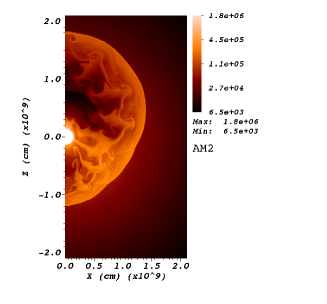
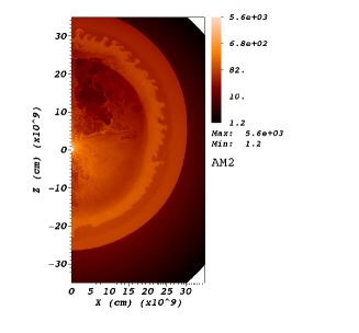
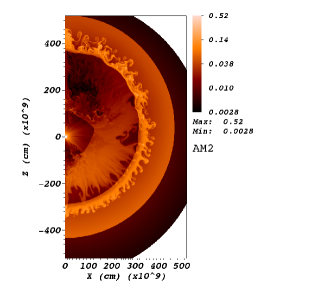
Figure 23.— Snap shots of distributions of density at the time of 0.572 s (top left), 30.0 s (top right), 711.5 s (bottom left), and 5753 s (bottom right) for model AM2. The unit of values in color bars is g cm^-3. The values in color bars are logarithmically scaled.

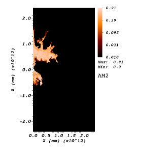
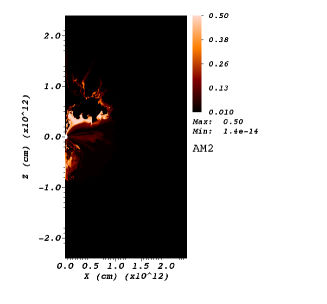
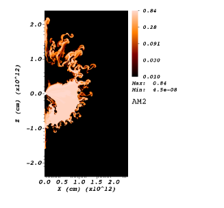
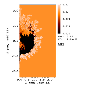
Figure 24.— Same as Figure 5 but for elements, ⁵⁶Ni, ²⁸Si, ¹⁶O, and ⁴He and the time of 4578 s.

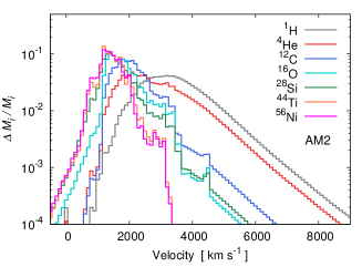
Figure 25.— Same as Figure 6 but for model AM2 at the time of 4578 s.

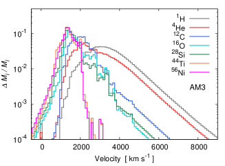
Figure 26.— Same as Figure 6 but for model AM3 at the time of 4562 s.

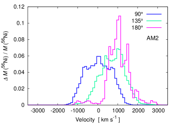
Figure 27.— Same as Figure 15 but for model AM2 and the time of 4578 s.

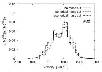
Figure 28.— Mass distributions of ⁵⁶Ni as a function of line of sight velocity ($\theta_{\rm ob}$ = 135^∘) at the end of simulation time (4578 s) for model AM2. Three cases without mass cut (solid), with the spherical mass cut (dashed), and with the aspherical mass cut (dotted) are shown. See the text in §5.1 for the explanation of the mass cut.

5. Discussion

5.1. Effects of the mass cut

In our calculations, the masses of ⁵⁶Ni in the computational domain at the end of simulation time are slightly overestimated compared with the value for SN 1987A (0.07 $M_{\odot}$: e.g., Shigeyama, Nomoto & Hashimoto, 1998). The obtained masses of ⁵⁶Ni range over 1.91 – 1.97 $\times$ 10^-1 $M_{\odot}$ for spherical models and model AT1. Those for the other models range over 7.23 $\times$ 10^-2 – 1.09 $\times$ 10^-1 $M_{\odot}$. The effects of the fallback of matter in our calculations may have some uncertainties because those could depend on the location of the inner boundary, the adopted inner boundary condition and the treatments of gravity. Therefore, in this section, we consider so-called the ‘mass cut’ which determines arbitrarily the location that divides the ejecta from the compact remnant. In the previous sections, we do not take into account the mass cut in deriving the mass of ⁵⁶Ni. Generally, the mass cut is determined so that the mass of ⁵⁶Ni in the ejecta is consistent with the observed one. We consider two types of the mass cut. One is the spherical mass cut which is determined to be the location that the sum of the mass of ⁵⁶Ni in from regions with larger radii to regions with smaller radii reaches 0.07 $M_{\odot}$. In this case the shape of the mass cut is almost spherical symmetric. The other is the aspherical mass cut which is determined to be the location that the sum of the mass of ⁵⁶Ni in from regions that have larger explosion energy (the sum of the specific kinetic, internal, and gravitational energies in the cell) to regions that have smaller explosion energy reaches 0.07 $M_{\odot}$ in a similar way in Nagataki (2000). The shape of the aspherical mass cut could be aspherical due to an aspherical explosion. Figure 28 shows the mass distributions of ⁵⁶Ni as a function of line of sight velocity ($\theta_{\rm ob}=$ 135^∘) at the end of simulation time for model AM2 with the effects of the mass cut. The case without mass cut is also depicted for reference. Both cases with the spherical mass cut (the dashed line) and aspherical mass cut (the dotted line), high velocity tails ($\gtrsim$ 1,000 km s^-1) are slightly enhanced compared with that without mass cut (the solid line). While the low velocity tails are slightly reduced compared with that without mass cut. The differences between the cases with the spherical mass cut and the aspherical mass cut are not much distinctive except for around the peak ($\sim$ 1,000 km s^-1). From the estimations in this section, we conclude that the effects of the mass cut on the results are not much large unless the total mass of ⁵⁶Ni is too overestimated.

5.2. Neutron star kick and its observational implication

As mentioned in §3.4, an aspherical explosion has been thought to be the one of promising triggers of neutron star (NS) kicks (e.g., Scheck et al., 2006; Wongwathanarat et al., 2010). The recoil velocity of a compact remnant (neutron star) can be estimated simply considering the momentum conservation. Initially, the total momentum of the progenitor is zero in the frame of the center of gravity (i.e., the center of the progenitor). Then, the neutron star recoil velocity is given by

$$\mbox{\boldmath$v$}_{\rm NS}\,(t)=-\mbox{\boldmath$P$}_{\rm gas}\,(t)/M_{\rm NS}\,(t),$$ (13)

where $\mbox{\boldmath$P$}_{\rm gas}=\int_{r_{\rm in}}^{r_{\rm out}}\rho\,\mbox{\boldmath$v$}\,dV$ is the total momentum outside the neutron star and $M_{\rm NS}$ is the mass of the neutron star. $r_{\rm in}$ ($r_{\rm out}$) is the radius of the inner (outer) boundary. We regard simply the mass of the neutron star $M_{\rm NS}$ as the mass inside the inner boundary. We estimate the recoil velocity of the compact remnant for model AM2. Note that since our simulations are axisymmetric, only $Z$-component has the non-zero value. The obtained neutron star velocity at the end of simulation time is $-\,734$ km s^-1. Since the sign is negative, the nascent neutron star is kicked in the opposite to stronger explosion direction. The averaged observed values of young pulsars are several hundred km s^-1 (e.g., Faucher-Giguère & Kaspi, 2006) and some of them have over 500 km s^-1, even 1,000 km s^-1 (Chatterjee et al., 2005). Therefore, the estimated value is within the observational values but it is somewhat larger than that of a typical one. In our estimation the values of $r_{\rm in}$ is rather larger than the surface radius of the compact remnant. Therefore, the estimated value may have large uncertainty. Hence, it is safe to say that our estimation includes uncertainty of several tens of % or more. Nonetheless, the estimated value may be within the observed range. From the analysis, the asymmetry roughly represented by $v_{\rm pol}/v_{\rm eq}$, $v_{\rm up}/v_{\rm down}=$ 2 may be sufficient to explain the observed velocities of young pulsars. For a typical velocity of young pulsars, $v_{\rm up}/v_{\rm down}<$ 2 may be preferable.

For SN 1987A, the compact remnant has not been found so far. However, if the explosion is stronger in some direction, the nascent neutron star will be kicked in the opposite to the strongest explosion direction as discussed above. Actually, the observed line profiles of [Fe II] as a function of Doppler velocity for SN 1987A are asymmetric across the null velocity point. The peak is located in the red-shifted side (Haas et al., 1990). It is commonly known that the images of SN 1987A have three rings. The inner ring is inclined at about 45^∘ to the sky, and the north (south) part of the ring is closer to (away from) us and blue-sifted (red-shifted) (e.g., Tziamtzis et al., 2011). Moreover, recent near infrared spectroscopic observations have revealed that the inner ejecta of SN 1987A is elongated and it is roughly confined to the same plane as the inner ring (Kjær et al., 2010). From above considerations, we can speculate the direction of the velocity of the compact remnant of SN 1987A. The south part of the explosion of SN 1987A is stronger than the north part of it because the south part of inner ejecta is red-shifted and the line profile of [Fe II] in SN 1987A implies that the explosion is stronger in the red-shifted side. Therefore, the compact remnant of SN 1987A may be kicked in a northern direction. It should be noted that a similar discussion have been done by Nagataki (2000) but the conclusion is opposite to ours. This may be because at that time, it had been thought that the explosion of SN 1987A had been a jetlike or bipolar and the north part of the inner ejecta of SN 1987A had been red-shifted (Wang et al., 2002). However, as noted above, recent observations contradict it.

The observed features of line profiles of [Fe II] in SN 1987A have not been excellently reproduced by not only our models but also recent previous studies with a neutrino-driven model (e.g., Kifonidis et al. (2006); Gawryszczak et al. (2010)). This is one of remained enigmas to be explained in the future. If the line profiles are reproduced by a more sophisticated model, it will be a good diagnostic to speculate the direction and magnitude of the recoil velocity of the compact remnant of SN 1987A.

5.3. Limitations of simulations and possible ingredients to obtain a higher velocity of ⁵⁶Ni

In this section, we consider the limitation of our simulations in the present paper and some possible ingredients to convey ⁵⁶Ni into higher velocity regions.

Self-gravity is implemented in our code assuming the spherical symmetry to save CPU time. However, as we have seen in previous sections, the distributions of density and mass fractions of metals are rather anisotropic and self-gravity due to anisotropic matter distributions could potentially affect the fallback and protrusions of innermost metals. Hence, it is desirable that the Poisson equation for self-gravity is solved in more sophisticated manner including multi-dimensional effects. Additionally, if matter distributions are changed from the results in the paper, it could affect the estimation of the recoil velocity of the nascent neutron star.

Energy depositions due to decays of radioactive nuclei ⁵⁶Ni and ⁵⁶Co are the one of possible mechanisms to accelerate innermost metals including ⁵⁶Ni in later phases after the shock breakout. If we assume the ejected mass of ⁵⁶Ni is 0.07 $M_{\odot}$, the total released energy estimated by Equations (5) and (6) reaches $\sim\,$1.3 $\times$ 10⁴⁹ erg 400 day after the explosion. In our models, the radial velocity of ⁵⁶Ni is clustered around 1,000 km s^-1 at the ends of simulation time. Hence, the kinetic energy of bulk ⁵⁶Ni is roughly estimated as

$$E_{\rm kin}\sim 1.6\times 10^{48}\,{\rm erg}\left(\frac{M}{0.07\,M_{\odot}}\right)\,\left(\frac{v}{1,000\,{\rm km\,s^{-1}}}\right)^{2}.$$ (14)

Therefore, if we assume that all the released energy from decaying ⁵⁶Ni and ⁵⁶Co is converted to the kinetic energy of itself, it becomes eight times larger than that before the heating, which corresponds to a threefold increase in velocity. Of course, part of the gamma-rays from the metals may escape without heating and the estimation of Equation (14) may have a large uncertainty. Then, the above estimation is kind of the upper bound. Nonetheless, the peak velocity of the ⁵⁶Ni could increase by about 30% due to decays of ⁵⁶Ni and ⁵⁶Co (Herant & Benz, 1991). As mentioned in §1, the heating due to the decay of ⁵⁶Ni and ⁵⁶Co could be the seed of perturbations in a later phase, i.e., ‘nickel bubble’. For SN 1987A, if 10% of ⁵⁶Ni ($\sim$ 0.007$M_{\odot}$) had $\sim$ 1,800 km s^-1 at the stage of $\sim$ 10⁴ s after the explosion, the velocity of ⁵⁶Ni of $\sim$ 3,000 km s^-1 could be explained (Basko, 1994). Our simulations are stopped just after the shock breakout due to the limitation of time. However, in order to determine the final velocity of ⁵⁶Ni, more long term simulations are required.

Three-dimensional effects could be the most important to convey innermost metals into high velocity regions. The differences of the growth of a single-mode perturbation between two- and three-dimension was investigated by Kane et al. (2000). The authors found that the growth of the perturbations in three-dimension is 30% – 35% faster than that in two-dimension. Hammer et al. (2010) demonstrated that the drag force to clumps of innermost metals in three-dimension is less than that in two-dimension. In their three-dimensional simulation, the clump can penetrate the dense helium shell (‘wall’) at the bottom of the hydrogen envelope even in the absence of RM instabilities. The authors insisted that in two-dimensional simulations, the motion of a clump is severely restricted to keep the ‘torus’-like structure due to the axisymmetric assumption, and the drag force to the clump becomes larger as the distance of the clump from the polar axis becomes larger. Therefore, our two-dimensional axisymmetric simulations may overestimate the drag force to clumps moving away from the polar axis, and protrusions of clumps of metals in a direction away form the polar axis could be changed in three-dimension. Joggerst et al. (2010b) investigated RT mixing in supernovae in three-dimension. Their finding is as follows. RT instabilities grow faster in three-dimension than in two-dimension at first, but in later phases, small-scale perturbations cause so-called ‘inverse cascading’, mergers of smaller-scale structures into larger-scale ones, in three-dimension, which reduce the local Atwood number , and eventually the resultant mixing lengths are not changed by the difference of the dimension. From the results of Hammer et al. (2010) and Joggerst et al. (2010b), the dimensional effects on matter mixing may be important only if the scale of perturbations is large.

In some models in the paper, outstanding protrusions of matter including ⁵⁶Ni along with the polar axis are seen. As mentioned before, those may reflect the combination of several effects as follows. 1. No penetration of matter across the polar axis due to the ‘reflection’ boundary condition. 2. Discretization errors close to the polar axis. 3. The physical nature that the explosions are the strongest in regions around the axis in our modes. However, as far as in two-dimensional axisymmetric simulation, we hardly know which point is the dominant effect. Moreover, Nordhaus et al. (2010) pointed out that strong bipolar asymmetry seen in two-dimensional neutrino-driven explosions aided by convection and/or SASI may not survive in three-dimension. Therefore, high-resolution, three-dimensional simulations are ultimately required to conclude the mixing of innermost metals and dimensional effects. We plan to extend our simulations for a prolonged time including multi-dimensional effects of self-gravity in the near future.

5.4. ⁴⁴Ti as an indicator of asphericity?

⁴⁴Ti is a relatively long-lived radioactive nucleus (the half life is 58.9$\pm$0.3 yr: Ahmad et al. (2006)) and accounts for the energy source of the light curve of a core-collapse supernova after the heating due to decays of ⁵⁶Ni and ⁵⁶Co cease. Inner ejecta of the remnant of SN 1987A may currently be heated due to decays of ⁴⁴Ti (Kjær et al., 2010). Recently, direct-escape lines from the decay of ⁴⁴Ti were detected in the remnant of SN 1987A (Grebenev et al., 2012). So far, direct-escape lines from the decay of ⁴⁴Ti have been clearly detected (e.g., Renaud et al., 2006) only in Cassiopeia A except for the remnant of SN 1987A. The obtained mass of ⁴⁴Ti at the ends of simulation time in our models range over 1.71 $\times$ 10^-4 – 5.16 $\times$ 10^-4 $M_{\odot}$. This is roughly consistent with the value (3.1$\pm$0.8) $\times$ 10^-4 $M_{\odot}$ derived from the detected direct-escape lines of ⁴⁴Ti in SN 1987A (Grebenev et al., 2012). ⁴⁴Ti is synthesized by incomplete silicon burning in the explosive nucleosynthesis. As mentioned in §1 and §4.2, ⁴⁴Ti is enhanced by an aspherical explosion due to the strong alpha-rich freeze-out (Nagataki et al., 1998a; Nagataki, 2000). We estimate the ratio of the masses of ⁴⁴Ti to ⁵⁶Ni. For spherical explosion models, the values are 1.24 $\times$ 10^-3. For bipolar explosion case, the values of models of $v_{\rm pol}/v_{\rm eq}$ = 2, are approximately 2.1 $\times$ 10^-3. While the values of models of $v_{\rm pol}/v_{\rm eq}$ = 4 are 2.57 $\times$ 10^-3. Therefore, models that have clear aspherical feature enhance the mass of ⁴⁴Ti relative to that of ⁵⁶Ni. For aspherical models of $v_{\rm pol}/v_{\rm eq}$ = 2 and $v_{\rm up}/v_{\rm down}$ = 2, the values range over 2.36 $\times$ 10^-3 – 5.22 $\times$ 10^-3. The value of representative model AM2 is 4.97 $\times$ 10^-3. Therefore, the values of models of $v_{\rm pol}/v_{\rm eq}$ = 2 and $v_{\rm up}/v_{\rm down}$ = 2 tend to be enhanced compared with those of bipolar explosion models. Note that the obtained mass of ⁴⁴Ti in our models may be overestimated due to the small nuclear reaction network. The mass of synthesized ⁴⁴Ti is roughly three orders of magnitude smaller than that of ⁵⁶Ni. Therefore, neglecting other elements in the network may more affect the mass fraction of ⁴⁴Ti than that of ⁵⁶Ni relatively. Therefore, the values of the ratio should be regarded as a guide. Nonetheless, the qualitative tendencies may be correct. Thus, the value of mass ratio of ⁴⁴Ti and ⁵⁶Ni could be a good indicator of the asphericity of the explosion.

6. Summary

We investigate matter mixing in a series of aspherical core-collapse supernova explosions of a 16.3 $M_{\odot}$ with a compact hydrogen envelope using a two-dimensional axisymmetric AMR hydrodynamic code, FLASH. We revisit RT mixing in spherical and/or mildly aspherical (bipolar jetlike) explosions with perturbations of pre-supernova origins. The effects of initial clumpy structures and multiply introduced perturbations are also studied. Our main findings are as follows.

In spherical explosion models, the obtained maximum velocities of ⁵⁶Ni range over 1,500 – 1,600 km s^-1 and the minimum velocities of ¹H range over 800 – 1,400 km s^-1. The growth of RT mixing depends on the timing that perturbations are introduced. If perturbations are introduced when the shock wave reaches the composition interface of C+O/He, RT instabilities grow around the interface of C+O/He. On the other hand, if perturbations are introduced just before the shock wave reaches the composition interface of He/H, RT instabilities grow around the interface of He/H. RT instabilities around the interface of C+O/He account for conveying innermost metals including ⁵⁶Ni into high velocity regions. While RT instabilities around the interface of He/H results in strong inward mixing of ¹H and which can explain observed minimum velocity of ¹H. Multiply introduced perturbations of pre-supernova origins, i.e., RT instabilities around the composition interfaces of both C+O/He and He/H, do not affect the maximum velocity of ⁵⁶Ni.

In the case of mildly aspherical bipolar explosions the qualitative features are the same as in the spherical models, and the maximum velocities of ⁵⁶Ni and the minimum velocities of ¹H range over 1,200 – 1,700 km s^-1, and 700 – 1,300 km s^-1, respectively. Both the maximum velocity of ⁵⁶Ni and the minimum velocity of ¹H are obtained in the model which has the most aspherical explosion ($v_{\rm pol}/v_{\rm eq}=$ 4) and perturbations are introduced two times. The growth of RT instabilities is enhanced slightly in the direction of stronger explosion. The distributions of elements, e.g., ⁵⁶Ni, ²⁸Si, ¹⁶O, and ⁴He, are rather different from those of spherical models. ⁵⁶Ni is concentrated on regions closer to the polar axis. On the other hand, bulk of ¹⁶O is concentrated in equatorial regions.

As a revisiting model, we consider the model that has a mild explosion $v_{\rm pol}/v_{\rm eq}=$ 2 with large perturbations (30% amplitude) around the composition interface of He/H. In this model rather high velocity of ⁵⁶Ni ($\sim$ 3,000 km s^-1) is obtained and strong inward mixing of ¹H can be explained simultaneously. However, if the same perturbations are introduced in initial radial velocities, the shape of perturbations can not survive up until the shock wave reaches at the interface of He/H, and eventually, no high velocity ⁵⁶Ni is obtained. This implies that if such large and clear perturbations survive or exist due to some unknown mechanisms, the high velocity of ⁵⁶Ni around 3,000 km s^-1 can be reproduced.

To mimic a neutrino-driven explosion aided by convection and/or SASI, aspherical explosions asymmetric across the equatorial plane ($v_{\rm up}/v_{\rm down}=$ 2) with clumpy structures in initial shock waves (30% amplitude) are investigated. The obtained maximum velocities of ⁵⁶Ni and minimum velocity of ¹H range over 1,800 – 2,200 km s^-1 and 900 – 1,300 km s^-1, respectively. Overall the maximum velocities of ⁵⁶Ni are larger than those of bipolar explosion models but strong inward mixing of ¹H are not obtained. The protrusions of ⁵⁶Ni into the dense helium shell are sensitive to sizes of initial clumps. However, without RT instabilities due to perturbations of pre-supernova origins, the obtained maximum velocity of ⁵⁶Ni does not reach the observed level.

Finally, the combination of multiply introduced perturbations of pre-supernova origins and the aspherical explosion asymmetric across the equatorial plane with clumpy structures can cause the high velocity of ⁵⁶Ni (3,000 km s^-1) without strong RM instabilities around the composition interface of H/He.

To obtain a higher velocity of ⁵⁶Ni ($\sim$ 4,000 km s^-1), some additional ingredients may be required. As mentioned before, in two-dimensional axisymmetric simulations, it is difficult to assess whether features seen along the polar axis are realistic or not. Therefore, to conclude the mixing of innermost metals and final velocity of ⁵⁶Ni, more robust long-term, ultimately three-dimensional, simulations are required.

References

- Ahmad et al. (2006) Ahmad, I., Greene, J. P., Moore, E. F., et al. 2006, Phys. Rev. C, 74, 065803
- Arnett et al. (1989) Arnett, D., Fryxell, B., & Müller, E. 1989, ApJ, 341, L63
- Arnett & Meakin (2011) Arnett, W. D., & Meakin, C. 2011, ApJ, 733, 78
- Bader & Deuflhard (1983) Bader, G., & Deuflhard, P. 1983, Numer. Math., 41, 373
- Basko (1994) Basko, M. 1994, ApJ, 425, 264
- Bazán & Arnett (1998) Bazán, G., & Arnett, D. 1998, ApJ, 496, 316
- Benz & Thielemann (1990) Benz, W., & Thielemann, F.-K. 1990 ApJ, 348, L17
- Bethe (1990) Bethe, H. A. 1990, Rev. Mod. Phys., 62, 801
- Blinnikov et al. (2000) Blinnikov, S., Lundqvist, P., Bartunov, O., Nomoto, K., & Iwamoto, K. 2000, ApJ, 532, 1132
- Burrows et al. (2007) Burrows, A., Dessart, L., Livne, E., Ott, C. D., & Murphy, J. 2007, ApJ, 664, 416
- Chatterjee et al. (2005) Chatterjee, S., Vlemmings, W. H. T., Brisken, W. F., et al. 2005, ApJ, 630, L61
- Chevalier (1979) Chevalier, R. A. 1976, ApJ, 207, 872
- Colella & Woodward (1984) Colella, P., & Woodward, P. R. 1984, Journal of Computational Physics, 54, 174
- Couch et al. (2009) Couch, S. M., Wheeler, J. C., & Milosavljević, M. 2009, ApJ, 696, 953
- Delaney et al. (2010) Delaney, T., Rudnick, L., Stage, M. D., et al. 2010, ApJ, 725, 2038
- Dotani et al. (1987) Dotani, T., Hayashida, K., Inoue, H., et al. 1987, Nature, 330, 230
- Duff et al. (1986) Duff, I. S., Erisman, A. M., & Reid, J. K. 1986, Direct Methods for Sparse Matrices (Oxford: Clarendon Press)
- Ebisuzaki et al. (1989) Ebisuzaki, T., Shigeyama, T., & Nomoto, K. 1989, ApJ, 344, L65
- Ellinger et al. (2012) Ellinger, C. I., Young, P. A., Fryer, C. L., & Rockefeller, G. 2012, ApJ, 755, 160
- Fassia et al. (1998) Fassia, A., Meikle, W. P. S., Geballe, T. R., et al. 1998, MNRAS, 299, 150
- Faucher-Giguère & Kaspi (2006) Faucher-Giguère, C.-A., & Kaspi, V. M. 2006, ApJ, 643, 332
- Fryxell et al. (1991) Fryxell, B., Müller, E., & Arnett, D. 1991, ApJ, 367, 619
- Fryxell et al. (2000) Fryxell, B., Olson, K., Ricker, P., et al. 2000, ApJS, 131, 273
- Fujimoto et al. (2007) Fujimoto, S., Hashimoto, M., Kotake, K., & Yamada, S. 2007, ApJ, 656, 382
- Fujimoto et al. (2008) Fujimoto, S., Nishimura, N., & Hashimoto, M. 2008, ApJ, 680, 1350
- Gawryszczak et al. (2010) Gawryszczak, A., Guzman, J., Plewa, T., & Kifonidis, K. 2010, A&A, 521, A38
- Grebenev et al. (2012) Grebenev, S. A., Lutovinov, A. A., Tsygankov, S. S., & Winkler, C. 2012, Nature, 490, 373
- Haas et al. (1990) Haas, M. R., Colgan, S. W. J., Erickson E. F., et al. 1990, ApJ, 360, 257
- Hanuschik et al. (1988) Hanuschik, R. W., Thimm, G., & Dachs, J. 1988, MNRAS, 234, 41
- Hachisu et al. (1990) Hachisu, I., Matsuda, T., Nomoto, K., & Shigeyama, T. 1990, ApJ, 358, L57
- Hachisu et al. (1992) Hachisu, I., Matsuda, T., Nomoto, K., & Shigeyama, T. 1992, ApJ, 390, 230
- Hammer et al. (2010) Hammer, N. J., Janka, H.-Th., & Müller, E. 2010, ApJ, 714, 1371
- Herant & Benz (1991) Herant, M., & Benz, W. 1991, ApJ, 370, L81
- Herant & Benz (1992) Herant, M., & Benz, W. 1992, ApJ, 387, 294
- Hungerford et al. (2005) Hungerford, A. L., Fryer, C. L., & Rockefeller, G. 2005, ApJ, 635, 487
- Hungerford et al. (2003) Hungerford, A. L., Fryer, C. L., & Warren, M. S. 2003, ApJ, 594, 390
- Janka (2012) Janka, H.-Th. 2012, Annual Review of Nuclear and Particle Science, 62, 407
- Joggerst et al. (2010a) Joggerst, C. C., Almgren, A., Bell, J., et al. 2010a, ApJ, 709, 11
- Joggerst et al. (2010b) Joggerst, C. C., Almgren, A., & Woosley, S. E. 2010b, ApJ, 723, 353
- Joggerst et al. (2009) Joggerst, C. C., Woosley, S. E., & Heger, A. 2009, ApJ, 693, 1780
- Kane et al. (2000) Kane, J., Arnett, D., Remington, B. A., et al. 2000, ApJ, 528, 989
- Kifonidis et al. (2003) Kifonidis, K., Plewa, T., Janka, H.-Th., & Müller, E. 2003, A&A, 408, 621
- Kifonidis et al. (2006) Kifonidis, K., Plewa, T., Scheck, L., Janka, H.-Th., & Müller, E. 2006, A&A, 453, 661
- Kjær et al. (2010) Kjær, K., Leibundgut, B., Fransson, C., Jerkstrand, A., & Spyromilio, J. 2010, A&A, 517, A51
- Kotake et al. (2004) Kotake, K., Sawai, H., Yamada, S., & Sato, K. 2004, ApJ, 608, 391
- Kotake et al. (2006) Kotake, K., Sato, K., & Takahashi, K. 2006, Rep. Prog. Phys., 69, 971
- Kotake et al. (2012) Kotake, K., Takiwaki, T., Suwa, et al. 2012, Advances in Astronomy, 2012, 428757
- Kozma & Fransson (1998) Kozma, C., & Fransson, C. 1998, ApJ, 497, 431
- Löhner (1987) Löhner, R. 1987, Computational Methods in Applied Mechanics and Engineering, 61, 323
- Matz et al. (1988) Matz, S. M., Share, G. H., Leising, M. D., et al. 1988, Nature, 331, 416
- MacNeice (2000) MacNeice, P., Olson, K. M., Mobarry, C., de Fainchtein, R., & Packer, C. 2000, Computer Physics Communications, 126, 330
- Marek & Janka (2009) Marek, A., & Janka, H.-Th. 2009, ApJ, 694, 664
- Müller et al. (1991) Müller, E., Fryxell, B., & Arnett, D. 1991 A&A, 251, 505
- Nagataki (2000) Nagataki, S. 2000, ApJS, 127, 141
- Nagataki et al. (1997) Nagataki, S., Hashimoto, M., Sato, K., & Yamada, S. 1997, ApJ, 486, 1026
- Nagataki et al. (2006) Nagataki, S., Mizuta, A., & Sato, K. 2006, ApJ, 647, 1255
- Nagataki et al. (2003) Nagataki, S., Mizuta, A., Yamada, S., Takabe, H., & Sato, K. 2003, ApJ, 596, 401
- Nagataki et al. (1998a) Nagataki, S., Hashimoto, M., Sato, K., Yamada, S., & Mochizuki, Y. S. 1998a, ApJ, 492, L45
- Nagataki et al. (1998b) Nagataki, S., Shimizu, T. M., & Sato, K. 1998b, ApJ, 495, 413
- Nishimura et al. (2006) Nishimura, S., Kotake, K. Hashimoto, M., et al. 2006, ApJ, 642, 410
- Nomoto & Hashimoto (1988) Nomoto, K., & Hashimoto, M. 1988, Phys. Rep., 163, 13
- Nordhaus et al. (2010) Nordhaus, J., Burrows, A., Almgren, A., & Bell, J. 2010, ApJ, 720, 694
- Ono et al. (2009) Ono, M., Hashimoto, M., Fujimoto, S. Kotake, K., & Yamada, S. 2009, Prog. Theor. Phys., 122, 755
- Ono et al. (2012) Ono, M., Hashimoto, M., Fujimoto, S. Kotake, K., & Yamada, S. 2012, Prog. Theor. Phys., 128, 741
- Quirk (1997) Quirk, J. J. 1997, in Upwind and High-Resolution Schemes, ed. M. Yousuff Hussaini, Bram van Leer & John Van Rosendale (Berlin: Springer)
- Renaud et al. (2006) Renaud, M., Vink, J., Decourchelle, A., et al. 2006, ApJ, 647, L41
- Sawai et al. (2005) Sawai, H., Kotake, K., & Yamada, S. 2005, ApJ, 631, 446
- Sedov (1959) Sedov, L. I. 1959, Similarity and Dimensional Methods in Mechanics (New York: Academic Press)
- Scheck et al. (2006) Scheck, L., Kifonidis, K. Janka, H.-Th., & Müller, E. 2006, A&A, 457, 963
- Shigeyama & Nomoto (1990) Shigeyama, T., & Nomoto, K. 1990, ApJ, 360, 242
- Shigeyama, Nomoto & Hashimoto (1998) Shigeyama, T., Nomoto, K., & Hashimoto, M. 1988, A&A, 196, 141
- Spyromilio (1991) Spyromilio, J. 1991, MNRAS, 253, 25
- Spyromilio (1994) Spyromilio, J. 1994, MNRAS, 266, L61
- Spyromilio et al. (1990) Spyromilio, J., Meikle, W. P. S., & Allen, D. A. 1990, MNRAS, 242, 669
- Steffen (1990) Steffen, M. 1990, A&A, 239, 443
- Suwa et al. (2010) Suwa, Y., Kotake, K., Takiwaki, T., et al. 2010, PASJ, 62, L49
- Sunyaev et al. (1987) Sunyaev, R., Kaniovsky, A., Efremov, V., et al. 1987, Nature, 330, 227
- Takiwaki et al. (2009) Takiwaki, T., Kotake, K., & Sato, K. 2009, ApJ, 691, 1360
- Takiwaki et al. (2012) Takiwaki, T., Kotake, K., & Suwa, Y. 2012, ApJ, 749, 98
- Taylor (1946) Taylor, G. I. 1946, R. Soc. Lond. Proc. Ser. A, 186, 273
- Timmes & Swesty (2000) Timmes, F. X., & Swesty, F. D. 2000, ApJS, 126, 501
- Tziamtzis et al. (2011) Tziamtzis, A., Lundqvist, P., Gröningsson, P., & Nasoudi-Shoar, S. 2011, A&A, 527, A35
- Utrobin et al. (1995) Utrobin, V. P., Chugai, N. N., & Andronova, A. A. 1995, A&A, 295, 129
- Utrobin (2004) Utrobin, V. P. 2004, Astronomy Letters, 30, 293
- Wang et al. (2002) Wang, L., Wheeler, J. C., Höflich, P., et al. 2002, ApJ, 579, 671
- Weaver et al. (1978) Weaver, T. A., Zimmerman, G. B., & Woosely, S. E. 1978, ApJ, 225, 1021
- Winteler et al. (2012) Winteler, C., Käppeli, R. Perego, A., et al. 2012, ApJ, 750, L22
- Wongwathanarat et al. (2010) Wongwathanarat, A., Janka, H.-Th., & Müller, E. 2010, ApJ, 725, L106
- Woosely (1988) Woosley, S. E. 1988, ApJ, 330, 218
- Yamada & Sato (1991) Yamada, S., & Sato, K. 1991, ApJ, 382, 594