Direct Numerical Simulation of Electrokinetic Instability and Transition to Chaotic Motion

Abstract

A new type of instability — electrokinetic instability — and an unusual transition to chaotic motion near a charge-selective surface (semi-selective electric membrane, electrode or system of micro-/nanochannels) was studied by numerical integration of the Nernst-Planck-Poisson-Stokes system and a weakly nonlinear analysis near the threshold of instability. A special finite-difference method was used for the space discretization along with a semi-implicit $3\frac{1}{3}$-step Runge-Kutta scheme for the integration in time. The linear stability problem was resolved by a spectral method. Two kinds of initial conditions were considered: (a) white noise initial conditions to mimic “room disturbances” and subsequent natural evolution of the solution; (b) an artificial monochromatic ion distribution with a fixed wave number to simulate regular wave patterns. The results were studied from the viewpoint of hydrodynamic stability and bifurcation theory. The threshold of electroconvective movement was found by the linear spectral stability theory, the results of which were confirmed by numerical simulation of the entire system. The following regimes, which replace each other as the potential drop between the selective surfaces increases, were obtained: one-dimensional steady solution; two-dimensional steady electroconvective vortices (stationary point in a proper phase space); unsteady vortices aperiodically changing their parameters (homoclinic contour); periodic motion (limit cycle); and chaotic motion. The transition to chaotic motion did not include Hopf bifurcation. Numerical resolution of the thin concentration polarization layer showed spike-like charge profiles along the surface, which could be, depending on the regime, either steady or aperiodically coalescent.

The numerical investigation confirmed the experimentally observed absence of regular (near-sinusoidal) oscillations for the overlimiting regimes. There is a qualitative agreement of the experimental and the theoretical values of the threshold of instability, the dominant size of the observed coherent structures, and the experimental and theoretical volt–current characteristics.

I Introduction

I.1 General background

Problems of electrokinetics have recently attracted a great deal of attention due to rapid developments in micro-, nano- and biotechnology. Among the numerous modern applications of electrokinetics are micropumps, biological cells, electropolishing of mono- and polycrystalline aluminum, and the growth of aluminum oxide layers for creating micro- and nanoscale regular structures such as quantum dots and wires.

The study of the space charge in the electric double-ion layer in an electrolyte solution between semi-selective ion-exchange membranes under a potential drop is a fundamental problem of modern physics, first addressed by Helmholtz. The first theoretical investigation of the regime of limiting currents was done in the works by Grafov and Chernenko GrCh1 , Smyrl and Newman Smr1 and Dukhin and Deryagin DukhDe . Rubinstein and Shtilman Rub1 described the regime of limiting currents (see also Buk1 ; Nik1 ; Lis1 ; Man1 ; Bab5 ; Chu1 ). Hydrodynamics is not involved in either the underlimiting or limiting regime, and both regimes are one-dimensional. A curious electrokinetic instability and pattern formation were theoretically predicted by Rubinstein and Zaltzman [Rub3, ,Rub10, ] as a bifurcation to overlimiting regimes, which also makes the solution two-dimensional. Rubinstein, Staude and Kedem Rub23 found experimentally that the transition to the overlimiting regime was accompanied by current oscillations. These facts indirectly indicated a correlation between the instability and overlimiting currents. This correlation was also demonstrated in Maletzki et al. Mal , Belova et al. Belv , and Rubinstein et al. Rub12 , where the overlimiting regimes were eliminated when instability was artificially suppressed. The first direct experimental proof of the electroconvective instability that arises with an increasing potential drop between the bulk ion-selective membranes was reported by Rubinstein et al. RubRub1 , who managed to show the existence of small vortices near the membrane surface. Yossifon and Chang YCh also observed an array of electroconvective vortices arising under the effect of a slow alternating electric field, while Kim et al. KmHn found a nonequilibrium vortices DC field. A unified theoretical description of electrokinetic instability, valid for all three regimes, was presented by Zaltzman and Rubinstein Rub13 , based on a systematic asymptotic analysis of the problem. The numerical analysis of the nonlinear regimes of the electrokinetic instability was developed in DemShel ; DemChang ; Han1 . The self-similar character of the initial stage of the evolution and instability of the self-similar solution were investigated in DemShel ; KD2 ; DemSh ; Dem .

I.2 Electrokinetic instability

The fundamental interest in the problem is connected with a novel type of electrohydrodynamic instability: electrokinetic instability. This instability triggers a hydrodynamic flow and, in turn, intensifies the ion flux, which is responsible for the overlimiting currents. Although the cells observed in the electroconvective motion look like the cells in Rayleigh-Bénard convection and Bénard-Marangoni thermoconvection, the electroconvective instability is much more complicated from both the physical and the mathematical points of view. The Reynolds number in the electrokinetic instability is very small and, hence, the dissipation is very large and the nonlinear terms in Navier-Stokes system are negligibly small. The nonlinearity responsible for bifurcation arises from other equations of the system (Nernst-Planck-Poisson-Stokes system). This explains the dramatic distinction between the chaotic motion in the macro- and microhydrodynamics. The electrohydrodynamics of the electrolytes between the membranes manifests new types of bifurcation and transition to chaos, developed in both micro- and nanoscales. In particular, the large dissipation of the system should suppress its oscillatory motion, in particular, Hopf bifurcation. In Fig. 1, the results of experiments VNic1 do not reveal any of the regular sinusoidal behavior that is characteristic near a Hopf bifurcation point.

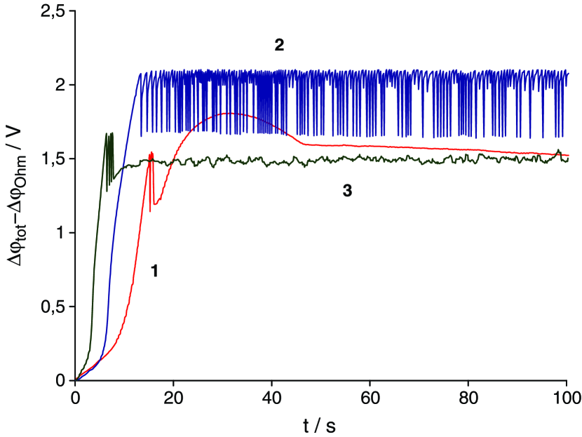
Figure 1: (Color online) Chronopotentiograms time vs voltage in $NaCl$ solutions at different ratios of the current density to its limiting value: 1 — 1.5; 2 — 2.5; 3 — 3.6 VNic1

I.3 Numerical tools and methods of the present work

During the last decades, direct numerical simulations have been recognized as a powerful and reliable tool for studying many classical hydrodynamical problems, in particular, for modeling laminar–turbulent transitions and chaotic turbulent flows. It is then logical to apply this tool to study electrokinetic instability. The system of the Nernst-Planck-Poisson-Stokes equations has a small parameter, the Debye number, at the highest derivatives. As a result, a thin space charge region with a rapid changing of the unknowns is formed near the surface. This causes significant difficulties for its numerical solution. These difficulties are compounded by the complexity of the chaotic regime when the flow contains a wide range of different scales. There are two approaches to overcoming these difficulties. The first one is semi-analytical, when the solution in the extended space charge region is sought analytically as the inner expansion but numerically in the diffusion region which is treated as the outer expansion, with a proper matching of the inner and outer expansions, see [Rub10, ,Pun2, ]. The second approach solves the entire system of Nernst-Planck-Poisson-Stokes equations numerically, without any simplification. In this case, the extensive experience of turbulent flow simulation for the Navier-Stokes equations can be employed.

In our previous works, [DemShel, ,DemChang, ], a quasi-spectral discretization with Fourier series and Chebyshev polynomials was applied in the spatial directions; this method happened to be computer time consuming. In the present work, a special finite-difference scheme with a grid point accumulation in the extended space charge region near the wall has been developed.

Spatial discretization with fine resolution leads to stiff problems and requires implicit methods for time advancement. Fully implicit methods produce a set of nonlinear coupled equations for the problem variables on the new time level, and are usually prohibitively costly for long-term calculations. Semi-implicit methods, in which only a part of the operator is treated implicitly, constitute a reasonable compromise for this class of problems.

A semi-implicit three-step Runge-Kutta scheme with third-order accuracy in time was adopted from Niki1 ; Niki2 ; NVN2 , where it was applied to the unsteady Navier-Stokes equations. The scheme is supplied with a built-in local accuracy estimation and time-step control algorithm. The idea of the time-step control algorithm is not novel. It was first utilized in semi-implicit Runge-Kutta schemes for the Navier-Stokes equations in [Niki3, ,Niki4, ]. Having been extensively exploited for a period of about 10 years, it proved itself to be efficient and convenient, especially for flows with wide variations in characteristic time scales, for instance, in simulations of laminar–turbulent transitions.

The results of the extensive numerical simulation are discussed and understood from the viewpoint of bifurcation theory. Two kinds of initial conditions have been considered: artificial monochromatic perturbations and white noise initial conditions to mimic natural room disturbances. The context of the present work is the set of attractors of a high dimensional dynamical system generated by the original Nernst-Planck-Poisson-Stokes equations. The averaged electric current and its time derivative have been taken as a representative low dimensional projection to describe the behavior of the whole system, its transitions, and attractors.

I.4 Outline

The present paper is structured as follows. In Part 2, the governing equations for the dilute electrolyte, the Nernst-Planck-Poisson-Stokes system, along with the relevant boundary and initial conditions (of two kinds) are presented in dimensionless form and typical characteristic values of the system parameters are evaluated.

Part 3 describes the details of the finite-difference scheme with respect to both the spatial variables and time. The selection of the domain length and discretization of the initial conditions are discussed at the end of Part 3.

Part 4 presents the results of the numerical simulation, and they are then discussed from the viewpoint of bifurcation theory and hydrodynamic stability. The potential drop $\Delta V$ is taken as a control parameter, and the bifurcation points and corresponding regimes are investigated in terms of this parameter. At the end of this part, the results of the simulation are qualitatively compared with experiments.

Part 5 summarizes and discusses the research, and presents the main conclusions.

II The mathematical model

A symmetric, binary electrolyte with a diffusivity of cations and anions $\tilde{D}$, dynamic viscosity $\tilde{\mu}$ and electric permittivity $\tilde{\varepsilon}$, and bounded by an ideal, semi-selective ion-exchange membrane surfaces, $\tilde{y}=0$ and $\tilde{y}=\tilde{L}$, is considered. Notations with tilde are used for the dimensional variables, as opposed to their dimensionless counterparts without tilde. $\{\tilde{x},\tilde{y}\}$ are the coordinates, where $\tilde{x}$ is directed along the membrane surface and $\tilde{y}$ is normal to the membrane surface.

The characteristic quantities to make the system dimensionless are:
$\tilde{L}$ — the characteristic length, the distance between the membranes; $\tilde{L}^{2}/\tilde{D}$ — the characteristic time; $\tilde{\mu}$ — the dynamic viscosity; $\tilde{\Phi}_{0}=\tilde{R}\tilde{T}/\tilde{F}$ — the thermodynamic potential; $\tilde{c}_{0}$ — the bulk ion concentration at the initial time.
Here $\tilde{F}$ is Faraday’s constant, $\tilde{R}$ is the universal gas constant and $\tilde{T}$ is the temperature in kelvins. In terms of the dimensional variables, the flow is confined between rigid walls at $y=0$ and $y=1$.

The electroconvection is described by the equations for the ion transport, the Poisson equation for the electric potential, and the Stokes equations for a creeping flow:

$$\frac{\partial c^{\pm}}{\partial t}+\mathbf{u}\cdot\nabla c^{\pm} = \pm\nabla\cdot\left(c^{\pm}\nabla\Phi\right)+\nabla^{2}c^{\pm},$$ (1)

$$\nu^{2}\nabla^{2}\Phi = c^{-}-c^{+}\quad\equiv-\rho,$$ (2)

$$-\nabla\Pi+\nabla^{2}\mathbf{u} = \frac{\varkappa}{\nu^{2}}\rho\nabla\Phi,\quad\nabla\cdot\mathbf{u}=0.$$ (3)

Here $c^{+}$ and $c^{-}$ are the molar concentrations of cations and anions; $\mathbf{u}=\{u,v\}$ is the fluid velocity vector; $\Phi$ is the electrical potential; $\Pi$ is the pressure; $\nu$ is the dimensionless Debye length or Debye number, which is the ratio of the Debye length $\tilde{\lambda}_{D}$ with the macroscopic length $\tilde{L}$,

$$\nu=\frac{\tilde{\lambda}_{D}}{\tilde{L}},\qquad\tilde{\lambda}_{D}=\left(\frac{\tilde{\varepsilon}\tilde{\Phi}_{0}}{\tilde{F}\tilde{c}_{0}}\right)^{1/2}=\left(\frac{\tilde{\varepsilon}\tilde{R}\tilde{T}}{\tilde{F}^{2}\tilde{c}_{0}}\right)^{1/2},$$

and $\varkappa$ is a coupling coefficient between the hydrodynamics and the electrostatics,

$$\varkappa=\frac{\tilde{\varepsilon}\tilde{\Phi}_{0}^{2}}{\tilde{\mu}\tilde{D}}.$$

It characterizes the physical properties of the electrolyte solution and is fixed for a given liquid and electrolyte.

If the flow is two-dimensional (2D), instead of the system (3), one equation for the stream function $\Psi$, $(u,v)=(\partial\Psi/\partial y,-\partial\Psi/\partial x)$, can be considered,

$$\nabla^{4}\Psi=\frac{\varkappa}{\nu^{2}}\left\{\frac{\partial}{\partial y}\left(\rho\frac{\partial\Phi}{\partial x}\right)-\frac{\partial}{\partial x}\left(\rho\frac{\partial\Phi}{\partial y}\right)\right\}.$$ (4)

The above system of equations is complemented by the proper boundary conditions:

$$y =0: c^{+} =p, \displaystyle-c^{-}\frac{\partial\Phi}{\partial y}+\frac{\partial c^{-}}{\partial y} =0, \Phi =0, \mathbf{u} =0;$$ (5)

$$y =1: c^{+} =p, \displaystyle-c^{-}\frac{\partial\Phi}{\partial y}+\frac{\partial c^{-}}{\partial y} =0, \Phi =\Delta V, \mathbf{u} =0.$$ (6)

The first boundary condition, prescribing an interface concentration equal to that of the fixed charges inside the membrane, is asymptotically valid for large $p$ and was first introduced by Rubinstein (see, for example, Rub13 and corresponding references) to avoid solution inside the membrane. The second boundary condition means no flux for negative ions, the third condition is a fixed potential drop, and the last condition is that the velocity vanish at the rigid surface. The spatial domain is assumed to be infinitely large in the $x$-direction, and the boundedness of the solution as $x\to\pm\infty$ is imposed as a condition.

Adding initial conditions for the cations and anions completes the system (1)–(6). These initial conditions arise from the following viewpoint: when there is no potential difference between the membranes, the distribution of ions is homogeneous and neutral. This corresponds to the condition $c^{+}=c^{-}=1$. Some kind of perturbation should be superimposed on this distribution,

$$t=0:\qquad c^{+}=1+\hat{c}^{+}(x),\qquad c^{-}=1+\hat{c}^{-}(x).$$ (7)

Two kinds of initial conditions (7) are considered.

(a) The initial conditions, which are natural from the viewpoint of the experiment. The so-called “room perturbations” determining the external low-amplitude and broadband white noise should be imposed on the concentrations. These initial conditions are

$$\hat{c}^{+}=\int_{0}^{\infty}\hat{p}(k)e^{-ikx}\,dk,\qquad\hat{c}^{-}=\int_{0}^{\infty}\hat{n}(k)e^{-ikx}\,dk.$$ (8)

(b) Artificial forced monochromatic perturbations with a fixed wave number $k_{s}$,

$$\hat{c}^{+}=\hat{p}\cdot\cos k_{s}x,\qquad\hat{c}^{-}=\hat{n}\cdot\cos k_{s}x.$$ (9)

The characteristic electric current $j$ at the membrane surface is referred to the limiting current, $j_{\lim}=4$,

$$j=\frac{1}{4}\left(c^{+}\frac{\partial\Phi}{\partial y}+\frac{\partial c^{+}}{\partial y}\right)\quad\text{for}\quad y=0.$$ (10)

It is also convenient for our further analysis to introduce the electric current averaged with respect to the membrane length $l$ and with respect to the time:

$$\langle j(t)\rangle=\frac{1}{l}\int_{0}^{l}j(x,t)\,dx,\quad J=\lim_{T\to\infty}\frac{1}{T}\int_{0}^{T}\langle j(t)\rangle\,dt.$$ (11)

The problem is characterized by three dimensionless parameters: $\Delta V$, $\nu$, which is a small parameter, and $\varkappa$. The dependence on the concentration, $p$, for the overlimiting regimes is practically absent and thus $p$ is not included in the mentioned parameters.

The problem was solved for $\nu=10^{-4}\div 10^{-3}$, $\varkappa=0.02\div 0.5$, and the dimensionless potential drop varied within $\Delta V=0\div 100$. In all calculations, $p=5$. (Some of the calculations were executed for $p=1$ and $p=2$. For the overlimiting regimes, the results coincide with a graphical accuracy with the ones for $p=5$.)

Just to provide perspective, the bulk concentration of the aqueous electrolytes varies in the range $\tilde{c}_{\infty}=1\div 10^{3}\text{ mol}/\text{m}^{3}$; the potential drop is about $\Delta\tilde{V}=0\div 5$ V; the absolute temperature can be taken as $\tilde{T}=300$ K; the diffusivity is about $\tilde{D}=2\cdot 10^{-9}\div 10^{-8}\text{ m}^{2}/\text{s}$; the distance between the electrodes $\tilde{L}$ is of the order of $0.5\div 1.5$ mm; the concentration value $\tilde{p}$ on the membrane surface must be much larger than $\tilde{c}_{\infty}$ and it is usually taken within the range from $5\tilde{c}_{\infty}$ to $10\tilde{c}_{\infty}$. The dimensional Debye layer thickness $\tilde{\lambda}_{D}$ varies in the range from 1 to 100 nm, depending on the concentration $\tilde{c}_{\infty}$.

III The numerical method

III.1 Discretization of the Nernst-Planck-Poisson-Stokes system

A finite-difference method with second-order accuracy is used for the spatial discretization of (1)–(3). In accordance with a standard staggered grid layout, all scalars ($c^{\pm},\rho,\Phi,\Pi$) are defined in the centers of the computational cells, while the velocity components are sought in the centers of the cell faces. The grid is stretched in the normal $y$-direction via a $\tanh$ stretching function in order to properly resolve the thin boundary layers attached to the membrane surfaces. A uniform grid is used in the homogeneous tangential $x$-direction. The discretization of the linear terms in (1)–(3) as well as the formulation of the boundary conditions are straightforward. The concrete expressions can be found elsewhere, in Niki2 for example. The nonlinear terms in (1), written in a divergent form $\mathbf{u}\cdot\nabla c^{\pm}\mp\nabla\cdot\left(c^{\pm}\nabla\Phi\right)\equiv\nabla\cdot\left(c^{\pm}(\mathbf{u}\mp\nabla\Phi)\right)$, are discretized by central differences with the use of a second-order interpolation of $c^{\pm}$ from the cell centers to the cell faces.

As a result of the spatial discretization, the problem is reduced to the solution of the set of ordinary differential equations:

$$\frac{dC}{dt}=F(C).$$ (12)

Here, the $2N$-dimensional vector $C(t)$ is composed of $N$ grid values of $c^{+}$ and $N$ grid values of $c^{-}$, where $N=N_{x}N_{y}$ is the total number of cells in the computational mesh and $N_{x}$ and $N_{y}$ are the numbers of grid points in the respective spatial directions. The vector function $F(C)$ in (12) includes the discretized nonlinear and linear terms of (1).

The grid functions $\Phi$ and $\mathbf{u}$ which are required for the calculation of $F$ are found for a given $C$ from the discretized Poisson equation (2) and discretized Stokes problem (3). These linear problems are solved using the fast Fourier transformation (FFT) in the homogeneous direction with subsequent solution of the resulting one-dimensional equations. Thus, the discretized Poisson and Stokes problems are solved exactly by direct methods without iteration.

Equation (12) represents a stiff problem when a fine spatial resolution is used. Explicit methods of time advancement are prohibitively ineffective for this problem. Fully implicit methods require the inversion of the nonlinear right-hand side operator $F(C)$ and thus are extremely costly. A reasonable compromise may be a semi-implicit method, where only a part (usually linear) of the operator $F(C)$ is treated implicitly. To clarify the idea of a semi-implicit method as applied to (12), let us consider the first-order accurate semi-implicit Euler method. The advancement from time instant $t_{0}$ to the time instant $t_{1}=t_{0}+\Delta t$ in this method is made according to the following equation:

$$\frac{C_{1}-C_{0}}{\Delta t}=F(C_{0})-LC_{0}+LC_{1}.$$ (13)

Here $C_{0}=C(t_{0})$ is the given vector and $C_{1}=C(t_{1})$ is to be found. The linear operator $LC$ is extracted from $F(C)$ and treated implicitly in order to make time integration procedure more stable. It is appropriate to rewrite (13) in the following equivalent form:

$$(I-\Delta tL)\Delta C=\Delta tF(C_{0}),\quad\Delta C=C_{1}-C_{0}$$ (14)

with $I$ as the identity operator: $IC\equiv C$. One can see that the scheme (14) possesses first-order accuracy for any operator $L$. Thus the concrete form of the implicit operator $L$ does not affect the formal accuracy of the scheme, but it does affect its stability. A proper choice of the implicit operator determines the performance of the method. One extreme form of $L$ is the zero operator $L\Delta C\equiv 0$ which makes the scheme (14) explicit. The opposite extreme is $L=J$, where $J=dF(C)/dC$ is the Jacobian matrix of the problem. Probably, $L=J$ ensures the most stable time integration and thus allows the largest possible value of the time step $\Delta t$. However, the solution of a linear algebraic system with a full matrix $(I-\Delta tL)$, which is what is involved in (14), becomes prohibitively costly. So, a compromise must be found where $L$ is reasonably simple (say, sparse or banded), so that (14) can be solved efficiently and at the same time $L$ must be in a some sense close to the Jacobian $J$. Closeness to the Jacobian means that $L$ must contain those terms of $J$ that are responsible for the stiffness of the problem.

In the present paper, the semi-implicit Runge-Kutta scheme with third-order accuracy from Niki1 is used for the time integration of (12). At each step of the time advancement, this scheme requires a triple calculation of the right-hand side function $F(C)$ and four solutions of a linear problem similar to (14). The scheme is equipped with an algorithm of local accuracy estimation and automatic time-step control. Such an option is especially useful when searching for an optimal form of implicit operator $L$. Since the minimum mesh size in the direction normal to the wall is typically two or even three orders of magnitude smaller than those in the tangential directions, the largest part of the stiffness of the problem is connected with the second derivatives in this direction, namely, with the terms approximating $\partial^{2}c^{\pm}/\partial y^{2}$ in the right-hand side of (1). If only these terms are treated implicitly, the (14) takes the form

$$\frac{\delta^{2}\Delta C}{\delta y^{2}}-\frac{1}{\Delta t}\Delta C=-F(C_{0})$$ (15)

where $\delta/\delta y$ stands for the finite-difference derivative in the $y$-direction. Eq. (15) presents a system with a three-diagonal matrix and is solved by the standard sweep method. The use of an implicit operator of the form (15) liberalizes the stability restrictions appreciably and raises the maximal permissible value of $\Delta t$ by a factor of $10^{3}\div 10^{4}$ over that of an explicit time advancement scheme at typical values of the problem and grid parameters used in the simulations.

Although a limited amount of simulation can be performed (and actually was performed) with the use of (15), the stability restrictions are still evident. By modifying the implicit operator it was found that the second important source of instability comes from the term approximating the wall-normal counterpart of the term $\pm\nabla\cdot(c^{\pm}\nabla\Phi)$ in the right-hand side of (1), namely, $\pm\delta(c^{\pm}\delta\Phi/\delta y)/\delta y$ (with partial derivatives $\partial/\partial y$ replaced with their finite-difference analogs $\delta/\delta y$). Taking in the last expression $c^{\pm}=c^{\pm}_{0}+\Delta c^{\pm}$ and linearizing near $c^{\pm}_{0}=c^{\pm}(t_{0})$ yields $\pm\delta(c^{\pm}_{0}\delta\Delta\Phi/\delta y+\Delta c^{\pm}\delta\Phi_{0}/\delta y)/\delta y$. Here $\Phi_{0}$ and $\Delta\Phi$ are linearly expressed in terms of $c^{\pm}_{0}$ and $\Delta c^{\pm}$, respectively, through the finite-difference analog of the Poisson equation (2). One more simplification which makes it feasible to add the last expression into the implicit operator is to neglect the derivatives along the tangential direction in the Poisson equation for $\Delta\Phi$. Thus, (14) with the modified implicit operator becomes the linear problem

$$\frac{\delta^{2}\Delta c^{\pm}}{\delta y^{2}}\pm\delta(c^{\pm}_{0}\delta\Delta\Phi/\delta y+\Delta c^{\pm}\delta\Phi_{0}/\delta y)/\delta y-\frac{1}{\Delta t}\Delta c^{\pm}=-F^{\pm}(C_{0});$$ (16)

$$\nu^{2}\frac{\delta^{2}\Delta\Phi}{\delta y^{2}}=\Delta c^{-}-\Delta c^{+}.$$ (17)

The linear system (16)–(17) has a sparse matrix and is solved with the use of the IMSL routine LSLXG. The use of (16)–(17) instead of (15) produces a further increase of $\Delta t$ by two orders of magnitude. Although solving (16)–(17) via the LSLXG routine is up to 10 times longer than solving (15), the overall advantage of using (16)–(17) instead of (15) is obvious.

III.2 Domain length and discretization of the initial conditions

For the natural “room disturbances” the infinite spatial domain was changed to the large enough finite domain that has length $l$, with the corresponding wave number $k=2\pi/l$. The condition that the solution should be bounded as $x\to\infty$ was changed to periodic boundary conditions. The length of the domain $l$ had to be taken large enough to make the solution independent of the domain size. The wave number $k$ was taken to be 1, while $k=0.5$ and $k=0.25$ were used to verify the results.

The initial conditions (8) in discrete form are

$$t=0:$$

$$c^{+}-1\approx\sum_{m=1}^{M}|\hat{p}(k_{m})|\exp{(-ik_{m}x+i\theta_{m}^{+})},\quad c^{-}-1\approx\sum_{m=1}^{M}|\hat{n}(k_{m})|\exp{(-ik_{m}x+i\theta_{m}^{-})},$$ (18)

where the integrals were approximated by the sum, $k_{m}=m\cdot k$, $k=k_{c}/M$, $k_{c}$ is the largest wave number taken into account, and $\theta_{m}^{\pm}$ are the phases of the complex amplitudes $\hat{p}$ and $\hat{n}$, which were set by the random number generator with a uniform distribution in the interval $[0,2\pi]$. It was assumed that the amplitudes $|\hat{p}|$ and $|\hat{n}|$ are zero above $k_{c}$ and equal to a certain small value describing the natural external noise inside the interval $0<k_{m}<k_{c}$. To mimic a broadband white noise in our calculations $|\hat{p}|=|\hat{n}|=10^{-6}$ were taken, but some of the calculations were carried out with initial perturbations 100 times larger: $|\hat{p}|=|\hat{n}|=10^{-3}$. All the calculations were limited by the final time $t_{\max}=6\div 45$, which corresponds to the dimensional time from $\tilde{t}_{\max}$ of 5 to 60 minutes. In most of the presented calculations, $\nu=10^{-3}$ was taken.

IV Simulation results

In this section the results of the simulation will be analyzed using the standard tools of the theories of hydrodynamic stability and nonlinear dynamical systems. Unless otherwise stated, $\nu=10^{-3}$ or $\nu=10^{-4}$.

IV.1 1D trivial solution and its stability

The simulations showed that for $\Delta V<\Delta V_{*}\approx 29.5$ one-dimensional steady solutions were realized. For $\partial/\partial t=\partial/\partial x=0$ the system (1)–(3) turns into

$$c^{+}\frac{d\Phi}{dy}+\frac{dc^{+}}{dy}=4j,\quad c^{-}\frac{d\Phi}{dy}+\frac{dc^{-}}{dy}=0,\quad\nu^{2}\frac{d^{2}\Phi}{dy^{2}}=c^{-}-c^{+}$$ (19)

with the boundary conditions

$$y=0:\quad c^{+}=p,\quad\Phi=0,\qquad y=1:\quad c^{+}=p,\quad\Phi=\Delta V,\qquad\int_{0}^{1}c^{-}dy=1.$$ (20)

This system describes the 1D solution, which is decoupled from the hydrodynamics, $u=v=0$. The first numerical solution was obtained in Rub1 for the asymptotical solution, $\nu\to 0$, see Bab5 ; Chu1 ; Rub12 . Fig. 2 shows typical profiles of $c^{\pm}$ and $\rho$ for the underlimiting and limiting regimes.

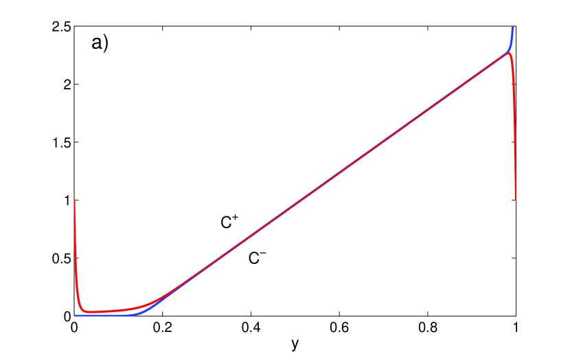
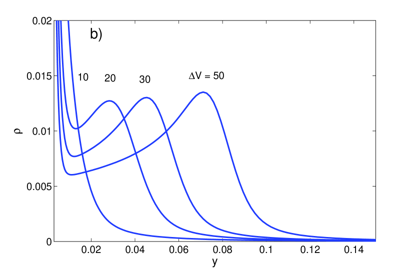
Figure 2: (Color online) 1D steady solution. Ion concentration for $\Delta V=25$, $\varkappa=0.1$ and $\nu=7\times 10^{-3}$ (a); charge density (b) near the membrane for $\nu=10^{-3}$, $\varkappa=0.1$ and different $\Delta V$

Numerical simulation of the full system (1)–(7) is in good agreement with the results obtained in Rub1 .

At $\Delta V=\Delta V_{*}$ the 1D solution (19)–(20) becomes unstable with respect to sinusoidal perturbations with wave number $k$,

$$c^{\pm}=c_{0}^{\pm}+\hat{c}^{\pm}\exp{(ikx+\lambda t)},\quad\Phi=\Phi_{0}+\hat{\Phi}\exp{(ikx+\lambda t)},\quad\Psi=\hat{\Psi}\exp{(ikx+\lambda t)}.$$ (21)

Suppose that these perturbations trigger a hydrodynamic flow, so that now $\Psi\neq 0$. The subscript $0$ is related to the mean 1D solution; hat, to perturbations. Upon linearization of (1)–(6) with respect to perturbations and omitting the subscript $0$ in the mean solution, we get the system

$$\lambda\hat{c}^{+}-ik\frac{dc^{+}}{dy}\hat{\Psi}=\frac{d}{dy}\left(c^{+}\frac{d\hat{\Phi}}{dy}+\frac{d\Phi}{dy}\hat{c}^{+}+\frac{d\hat{c}^{+}}{dy}\right)-k^{2}c^{+}\hat{\Phi}-k^{2}\hat{c}^{+},$$ (22)

$$\lambda\hat{c}^{-}-ik\frac{dc^{-}}{dy}\hat{\Psi}=\frac{d}{dy}\left(-c^{-}\frac{d\hat{\Phi}}{dy}-\frac{d\Phi}{dy}\hat{c}^{-}+\frac{d\hat{c}^{-}}{dy}\right)-k^{2}c^{-}\hat{\Phi}-k^{2}\hat{c}^{-},$$ (23)

$$\nu^{2}\left(\frac{d^{2}\hat{\Phi}}{dy^{2}}-k^{2}\hat{\Phi}\right)=\hat{c^{-}}-\hat{c^{+}}\equiv-\hat{\rho},$$ (24)

$$\frac{d^{4}\hat{\Psi}}{dy^{4}}-2k^{2}\frac{d^{2}\hat{\Psi}}{dy^{2}}+k^{4}\hat{\Psi}=ik\frac{\varkappa}{\nu^{2}}\left(\frac{d\rho}{dy}\hat{\Phi}-\frac{d\Phi}{dy}\hat{\rho}\right),$$ (25)

$$y=0:\quad\hat{\Phi}=0,\quad\hat{\Psi}=0,\quad\>\frac{d\hat{\Psi}}{dy}=0,\quad c^{-}\frac{d\hat{\Phi}}{dy}+\frac{d\Phi}{dy}\hat{c}^{-}-\frac{d\hat{c}^{-}}{dy}=0,\quad\hat{c}^{+}=0$$ (26)

$$y=1:\quad\hat{\Phi}=0,\quad\hat{\Psi}=\frac{d\hat{\Psi}}{dy}=0,\quad c^{-}\frac{d\hat{\Phi}}{dy}+\frac{d\Phi}{dy}\hat{c}^{-}-\frac{d\hat{c}^{-}}{dy}=0,\quad\hat{c}^{+}=0,$$ (27)

which is an eigenvalue problem for $\lambda$. If $\lambda(k)<0$ for all wave numbers $k$, the 1D solution (19)–(20) is stable; if $\lambda(k)>0$ for at least one $k$, the 1D solution is unstable and it gives the first bifurcation point of the system. The discretization was realized by expanding the unknown functions in Chebyshev series plus using the Lanczos procedure to satisfy the boundary conditions. The matrix eigenvalues were calculated by the QR-algorithm.

In all our calculations the $\lambda_{k}$ were real numbers, which means that the instability is monotonic. These eigenvalues are arranged in such a way that $\lambda_{1}>\lambda_{2}>\lambda_{3}>\dots$. The inset of Fig. 3 shows that for large $k$, $\lambda_{k}\sim k^{2}$. Fig. 3 pictures the marginal stability curves, $\lambda_{1}(k)=0$, in the plane $\Delta V-k$ for $\varkappa=0.1$ and various values of the parameter $\nu$.

The results of the numerical simulation of the nonlinear system (1)–(7) with the natural white noise initial conditions (8) are in good correspondence with the linear stability results which are presented in Table 1.

Table 1: Critical parameters for $\nu=10^{-3}$ and different $\varkappa$

$\varkappa$	0.02	0.05	0.10	0.15	0.20	0.50
$\Delta V_{*}$	55.0	38.0	29.5	25.5	23.5	19.1
$k_{*}$	4.65	4.7	4.8	4.9	5.0	5.1

Note that the numerical approach of Dem and the asymptotical approach Rub13 for small $\nu$ are also in good correspondence with the numerical simulation of the nonlinear system (our Debye number $\nu$ and the $\varepsilon$ used in Rub13 are related by $\varepsilon=\nu/\sqrt{2}$; the $Pe$-number of Rub13 is identical to our $\varkappa$). The transition to the primary instability to the critical point was approached both from below and from above in $\Delta V$, and no hysteresis was observed, indicating that the bifurcation is supercritical for the parameter values studied here.

The critical potential drop $\Delta V_{*}$ and critical wave number $k_{*}$ for different $\varkappa$ are presented in Table 1. The instability triggers an additional mechanism of ion transport by convection and, hence, it is reasonable to visualize this bifurcation in the volt–current (VC) characteristic, see Fig. 4. The VC characteristics for the underlimiting and limiting regimes (solid curve in the figure) are described by the system (19)–(20) and do not depend on the coupling coefficient $\varkappa$, because no hydrodynamics is involved in the process. The curves corresponding to the overlimiting regime and different $\varkappa$ depart from this solid line at different bifurcation points $\Delta V*$, depending on $\varkappa$. The smaller is $\varkappa$, the more distant is the branching point from the origin. The critical potential drop $\Delta V_{*}$ versus the coupling coefficient $\varkappa$ (see the inset to Fig. 4) shows that $\Delta V_{*}=\operatorname{const}_{1}+\operatorname{const}_{2}/\sqrt{\varkappa}$ can be used as a good interpolation relation. Increasing the coupling coefficient $\varkappa$, the plateau region of the limiting regimes decreases, and in the limit $\varkappa\to\infty$, $\Delta V_{*}\to 8.95$. Note that the last value approximately corresponds to the potential drop of the transition from underlimiting regimes to limiting regimes. The dependences for the critical drop of potential and wave number can be presented in the following form,

$$\nu=10^{-3},\quad\Delta V_{*}=8.95+\frac{6.52}{\sqrt{\varkappa}},\quad k_{*}-4.8=2(\varkappa-0.1).$$

The dependence of $k_{*}$ on $\varkappa$ is rather weak and, very roughly, $k_{*}\approx 4.8$ for all considered $\varkappa$. In order to get $k_{*}$ accurately, the spatial interval was doubled and even tripled.

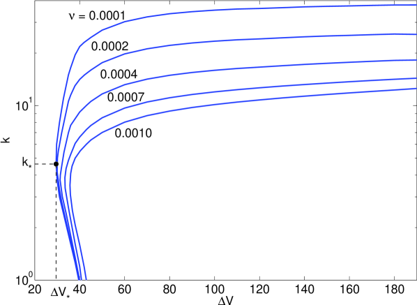
Figure 3: (Color online) Marginal stability curves $k$ vs $\Delta V$ for $\varkappa=0.1$ and different values of the parameter $\nu$. Inset: discrete spectrum $\{\lambda_{k}\}$ of the stability problem (22)–(27) for $k=4$, $\Delta V=29$, $\varkappa=0.1$ and $\nu=10^{-3}$

Figure 4: (Color online) VC characteristics for $\varkappa=0.2$ (diamonds), $0.1$ (triangles) and $0.05$ (circles) and $\nu=10^{-3}$. I, II, and III are the underlimiting, limiting, and overlimiting currents, respectively. The inset shows that $\Delta V_{*}$ linearly depends on $1/\sqrt{\varkappa}$; as $\varkappa\to\infty$, $\Delta V_{*}\to 8.94$

Table 2: Bifurcation points, $\varkappa=0.1$

$\vphantom{\Biggl{(}}\begin{array}[]{|c|c|c|c|}\hline\cr\Delta V_{*}&\Delta V_{**}&\Delta V_{***}\\ \hline\cr 29.5&32.5&37.0\\ \hline\cr\end{array}$

IV.2 Weakly nonlinear analysis and behavior near threshold

For the control parameter $\Delta V>\Delta V_{*}$ the uniform 1D state suffers a supercritical bifurcation. At the threshold of instability $k_{*}\neq 0$ and according to the classification of CrHog the instability is spatially periodic. Near $\Delta V_{*}$, $k_{*}$ the broadband initial spectrum (18) is filtered by the instability into a narrow band near the wave number $k_{*}$ and has a sinusoidal form with a slow envelope,

$$a\cdot e^{ik_{*}x}.$$

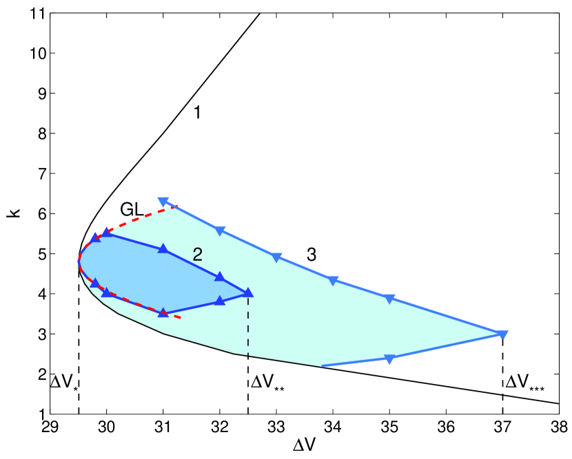
Figure 5: (Color online) Inside the curve 1 the trivial 1D solution is unstable; inside the region bounded by 2 there is a wave-number window of stable 2D steady solutions, this window according to GL-equation is marked in the figure as GL; for the region inside 3 the saddle value $S$ is negative. Triangles are taken from our simulation, $\varkappa=0.1$

For our kind of instability, near the point $\Delta V=\Delta V_{*}$ and $k=k_{*}$, the nonlinearities of the entire system (1)–(15) are weak and the spatial and temporal modulations of the basic linear stability pattern $ae^{ik_{*}x}$ are slow and their narrow band near $k_{*}$ is described by the weakly nonlinear Ginzburg-Landau (GL) equation (see [CrHog, ,WE, ]),

$$\frac{\partial a}{\partial t}=\gamma_{1}(\Delta V-\Delta V_{*})\cdot a+\gamma_{2}\frac{\partial^{2}a}{\partial x^{2}}-\gamma_{3}|a|^{2}a+\text{higher order terms}.$$ (28)

The first term in the right-hand side of the equation characterizes the instability and $\gamma_{1}$ is a real positive number. The second and third terms are responsible, respectively, for the dissipation and the nonlinear saturation, $\gamma_{2}$ and $\gamma_{3}$ for the common case are complex numbers, but in our case they are real numbers; these coefficients must be calculated numerically. Eq. (28) is valid for a small supercriticality, $\Delta V-\Delta V_{*}=\delta\to 0$. Upon rescaling the amplitude, time, and coordinate,

$$a=\left(\frac{\gamma_{1}}{\gamma_{3}}\right)^{1/2}\delta^{1/2}A,\quad\frac{\partial}{\partial t}=\gamma_{1}\delta\frac{\partial}{\partial\tau},\quad\frac{\partial^{2}}{\partial x^{2}}=\left(\frac{\gamma_{1}}{\gamma_{2}}\right)\delta\frac{\partial^{2}}{\partial\xi^{2}},$$

eq. (28) turns into

$$\frac{\partial A}{\partial\tau}=A+\frac{\partial^{2}A}{\partial\xi^{2}}-|A|^{2}A.$$ (29)

The 1D solution (19)–(20) corresponds to the trivial solution of (29), $A=0$. Eq. (29) also has the one-parameter family of nontrivial solutions,

$$A=\sqrt{1-\alpha^{2}}\cdot\exp({i\alpha\xi}),$$ (30)

with the parameter $\alpha$, $-1<\alpha<1$. This parameter is connected with the wave number $k$ by the relation

$$\alpha=\left(\frac{\gamma_{2}}{\gamma_{1}}\right)^{1/2}(k-k_{*})/\delta^{1/2}.$$ (31)

The solutions (30) are stable within the window $-\sqrt{3}/3<\alpha<\sqrt{3}/3$ (see CrHog ). Taking into account (31), this window can be recalculated to the stability region for the original wave number $k$,

$$k_{*}-\sqrt{\frac{\delta\gamma_{1}}{3\gamma_{2}}}<k<k_{*}+\sqrt{\frac{\delta\gamma_{1}}{3\gamma_{2}}}.$$ (32)

This stability domain is denoted by GL in Fig. 5.

IV.3 Family of 2D steady space-periodic solutions and their stability

Numerical simulations of the entire system (1)–(6) with the natural white noise initial conditions (8) confirmed the aforementioned predictions of the weakly nonlinear analysis: in some vicinity of the critical point, nonlinear saturation led to steady, $\partial/\partial t=0$, space-periodic 2D solutions. We call them steady periodical electroconvective vortices. For a very small supercriticality, these steady vortices behaved sinusoidally along the membrane surface, but with a small increase in $\Delta V$ above the critical potential drop (about 0.5% of $\Delta V_{*}$), the steady solution lost its sinusoidal profile along the $x$-coordinate and acquired a typical spike-like distribution. The neighboring vortices of opposite circulations carry a significant ion flux (for the space charge and stream-line distributions see Fig. 6(a)). The VC characteristic dramatically changes for the corresponding $\Delta V$ (see Fig. 4). The basic wave number of these solutions, $k_{s}$, along with its overtones, had nonzero Fourier amplitudes; all other Fourier modes which were not multiples of $k_{s}$ decayed to zero during the evolution. The value of the wave number $k_{s}$ depended upon a particular realization of the random-number generator (18).

Our next step was to extend the prediction of the weakly nonlinear analysis to finite supercriticality, namely: a) to build up a one-parameter family of these solutions with the parameter $k_{s}$; b) to find the region of stability of that family.

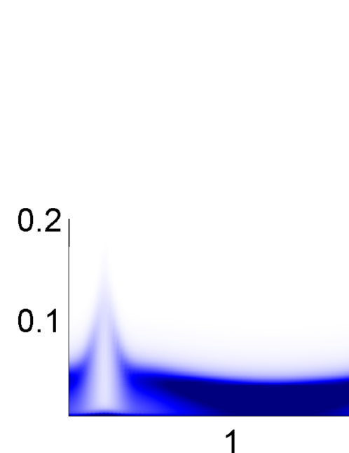
(a)

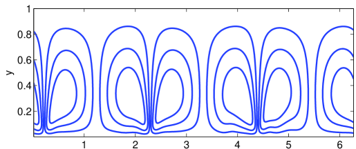
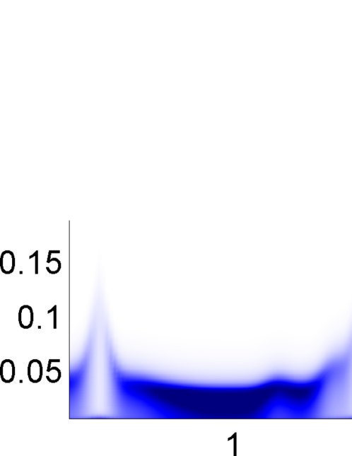
(b)

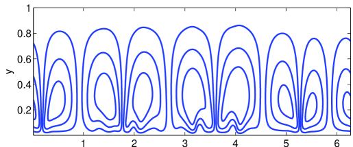
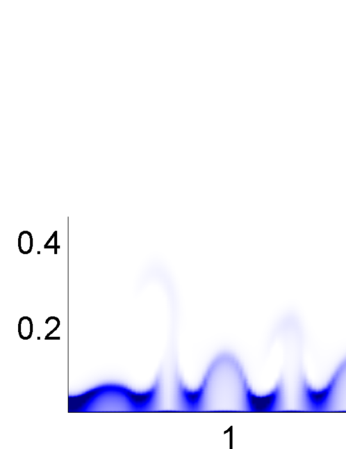
(c)

Figure 6: (Color online) Typical snapshots of the charge density $\rho(x,y,t)$ and the stream-lines $\psi(x,y,t)$ at the end of evolution; darker regions correspond to larger charge densities. (a) $\Delta V=31.5$, (b) $\Delta V=35$, (c) $\Delta V=50$, $\varkappa=0.1$ and $\nu=10^{-3}$

The problem of the stability of these two-dimensional solutions is much more difficult than for 1D solutions. If small perturbations are superimposed on the steady space-periodic solution of this family, these perturbations will be described by a system with time independent coefficients and will have period $2\pi/k_{s}$ in the $x$-coordinate. According to Floquet’s theorem, the elementary solution of this linear system, bounded at $x=\pm\infty$, has the form

$$G(x,y)\cdot\exp{(i\chi x)}\cdot\exp{(\mu t)},$$ (33)

where $G$ satisfies the corresponding boundary conditions at $y=0$ and $y=1$ and has the period $2\pi/k_{s}$ with respect to $x$, the wave number $\chi$ is a parameter which is changing within the interval, $0<\chi<k_{s}/2$, and, hence, includes side-band and subharmonic bifurcations, and $\mu$ is an eigenvalue of the problem.

Taking, in the simulations, small enough $k$ (or a large enough domain in $x$), we were able to study the problem numerically; $k$ was assumed to be a multiple of $k_{s}$, namely, there is an integer number $N$ such that $k\cdot N=k_{s}$. These perturbations can be described by the expansion

$$G=\psi_{1}(x,y)\cdot e^{\mu_{1}t}+\psi_{2}(x,y)\cdot e^{\mu_{2}t}+\psi_{3}(x,y)\cdot e^{\mu_{3}t}+\dots,$$ (34)

where $\psi_{k}$ are functions with period $2\pi/k$ in $x$, and $\{\mu_{k}\}$ are eigenvalues of the discrete spectrum. Such a stability analysis of space-periodic solutions for much simpler problems can be found, for example, in ChDemKop . The stability eigenvalues were ordered according to their real parts,

$$\Re{(\mu_{1})}>\Re{(\mu_{2})}>\Re{(\mu_{3})}>\dots$$

The first stability exponents $\mu_{1}$ and $\mu_{2}$ were found using the following algorithm.

1. The steady 2D solution for a given $k_{s}$ was calculated by numerically integrating (1)–(7) with the initial conditions (9), from $t=0$ to some $t=t_{0}$, until all transients decayed, and we were close enough to the steady state.

2. The solution found was duplicated $N$ times in the $x$-direction, so that its wave number was $k=k_{s}/N$. The calculations were restricted by $k=0.5$, which was small enough to find the long wave instability; the calculations were verified by doubling the $x$-domain, $k=0.25$.

3. Small random perturbations $\hat{f}^{\pm}(x,y)$ with $\hat{f}^{\pm}\sim 10^{-8}\div 10^{-6}$ were imposed on $c^{+}_{0}$ and $c^{-}_{0}$:

   $$t=t_{0}:\quad c^{+}=c^{+}_{0}+\hat{f}^{+}(x,y),\quad c^{-}=c^{-}_{0}+\hat{f}^{-}(x,y).$$ (35)

   The details of the space distribution of $\hat{f}^{\pm}$ did not affect the final result.

4. The system (1)–(6) with the initial conditions (35) was integrated for $t>t_{0}$ and simultaneously the mean square amplitude, $\varepsilon(t)$, was computed,

   $$\varepsilon(t)^{2}=\frac{k}{2\pi}\int_{0}^{1}\int_{0}^{2\pi/k}(c^{+}-c^{+}_{0})^{2}+(c^{-}-c^{-}_{0})^{2}\,dxdy,$$ (36)

   where $c^{\pm}_{0}$ were kept constant and the $c^{\pm}$ were functions of time.

Substitution of (34) into (36) results in the expansion

$$\varepsilon(t)=C_{1}\cdot e^{\mu_{1}t}+C_{2}\cdot e^{\mu_{2}t}+\dots\quad\text{for}\quad t\to\infty,$$ (37)

where $C_{k}$ are some constants. The typical behavior of $\varepsilon(t)$ for different $k_{s}$ is presented in Fig. 7 in semi-logarithmic coordinates, for large enough times $\log{\varepsilon(t)}\sim\mu_{1}t$. The first stability eigenvalue was obtained as a function of $k_{s}$; this function, $\mu_{1}(k_{s})$, is shown in Fig. 8 for different potential drops $\Delta V$. One can see that there is a window where the steady periodic solutions are stable. The boundary of this window is plotted in Fig. 5. For small supercriticality there is a reasonably good correspondence to the weakly nonlinear analysis. The stability balloon is finite, its right boundary for $\varkappa=0.1$, $\Delta V_{**}\approx 32.5$, see Fig. 5. In the region $\Delta V_{*}<\Delta V<\Delta V_{**}$, the eigenvalue $\mu_{1}$ is always a real number.

With the known $\mu_{1}$ we also managed to calculate the second eigenvalue $\mu_{2}$, using the following two-step procedure:

$$\text{(a)}\quad\varepsilon(t)\cdot e^{-\mu_{1}t}=C_{1}+C_{2}\cdot e^{(\mu_{2}-\mu_{1})t}+\dots,\quad\text{(b)}\quad\varepsilon(t)\cdot e^{-\mu_{1}t}-C_{1}=C_{2}\cdot e^{(\mu_{2}-\mu_{1})t}+\dots$$ (38)

The procedure for evaluating $\mu_{2}$ is illustrated in Fig. 7(b), and the dependence $\mu_{2}(k_{s})$ for different $\Delta V$ is given in Fig. 8. For $\Delta V<39$ all the eigenvalues $\mu_{2}$ are real and negative, but for $\Delta V>41$ all $\mu_{2}$ become positive (not shown in the figure).

IV.4 Homoclinic contours, their bifurcations, and the birth of chaos

For $\Delta V>\Delta V_{**}$ all the steady 2D vortices are unstable and the behavior becomes more complex. In order to clarify the behavior of the system it was instructive to consider its trajectories in the relevant phase space. The system has a phase space of high dimension, and it was crucial for its understanding to choose the proper projection of this space. The electric current averaged along the membrane, $\langle j\rangle$, and its time derivative, $d\langle j\rangle/dt$, seemed to be such a representative low-dimensional projection to characterize the different attractors.

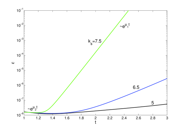
(a)
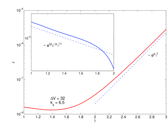
(b)

Figure 7: (Color online) Amplitude of perturbation vs time, $\varepsilon(t)$, for different wave numbers $k_{s}$ (a); scheme for evaluating the first eigenvalues of stability, $\mu_{1}$ and $\mu_{2}$, for $k_{s}=6.5$ (b); $\varkappa=0.1$, $\Delta V=34$

(a)
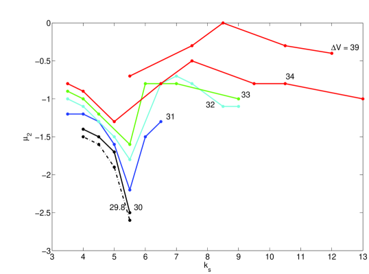
(b)

Figure 8: (Color online) Dependence of the first eigenvalues, $\mu_{1}$ and $\mu_{2}$, on the wave number $k_{s}$ for different $\Delta V$, $\varkappa=0.1$

For the regime of steady 2D vortices, $\Delta V_{*}<\Delta V<\Delta V_{**}$, the phase trajectory at $t\to\infty$ is attracted to some fixed point, $\langle j\rangle=\operatorname{const}$ and $d\langle j\rangle/dt=0$, with wave number $k_{s}$ from the stability interval, see Fig. 10(a). With increasing $\Delta V$, this stability interval narrows, and at $\Delta V=\Delta V_{**}$ shrinks to one point, for $\varkappa=0.1$ and $\nu=10^{-3}$, $k_{s}\approx 4$.

For $\Delta V>\Delta V_{**}$ the stability interval vanishes. All the stationary points become saddle-node points, making a one-dimensional unstable manifold which corresponds to the real eigenvalue $\mu_{1}>0$. After a long transition period there was established the behavior: (a) the phase trajectory was rapidly attracted to some saddle point along its stable manifold; (b) the solution spent a significant time near this stationary state; (c) the solution was rapidly expelled from the vicinity of the saddle point along its one-dimensional unstable manifold (d) with a subsequent return to the stationary saddle point, etc. The attracting–repelling scenario ran over many times. Return to the steady state was aperiodic; and with each new cycle, the time spent in the steady state increased. Apparently, the attractor of the system was a homoclinic contour, consisting of the saddle fixed point and trajectories doubly asymptotic to this point as $t\to\pm\infty$ (see, for example, GH ). The typical projections are shown in Fig. 10(b).

In the physical plane the behavior can be described as follows: the solution for a long time looked like a steady 2D electroconvective vortex; after this time the neighboring spikes of the space charge either merged quickly to create larger ones or disintegrated and broke up into smaller ones with a final return to the quasi-steady structure, etc. (see Fig. 6(b)). The wave number of this quasi-steady structure was $k_{s}\approx 2\div 4$.

The behavior for simpler dynamical systems with a saddle-node point is well known, see GH . The dynamics in the phase space of such a system is dominated by the saddle point, because the phase trajectory spends most of its time near this point. $S=\mu_{1}+\mu_{2}$ ($\mu_{1}>0$ and $\mu_{2}<0$) is called the saddle value. If $S$ is negative, this means that the saddle point “attracts stronger” than it “repels”. Then the attractor of the system is a homoclinic contour which consists of the saddle point and the loop which is the intersection of the stable and unstable manifolds of the saddle point. If $S$ is positive, this contour becomes unstable and what results from bifurcation from the homoclinic orbit limit cycle inherits stability.

Our problem is more complex, but its behavior seems to preserve the main features of the finite dynamical system with a homoclinic contour. We calculated the saddle value $S$ for $\Delta V>\Delta V_{**}$ and presented it in Fig. 9 as a function of the wave number $k_{s}$ for different potential drops. The boundary with $S=0$ is denoted in Fig. 5 by the line 3. The figure shows that for $\Delta V<\Delta V_{***}\approx 37$ there are saddle points with negative $S$, a fact which we interpret as the existence of stable homoclinic contours.

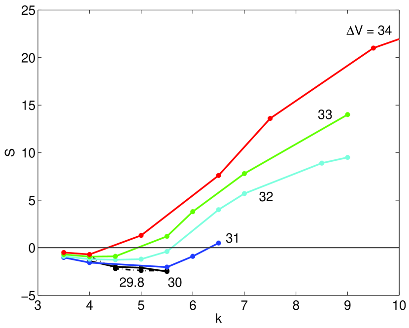
Figure 9: (Color online) Saddle value $S$ as a function of $k_{s}$ for different potential drops, $\varkappa=0.1$

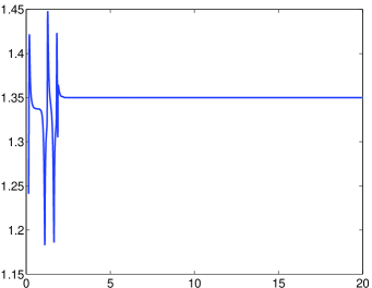
a)
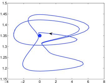
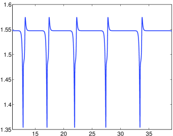
b)
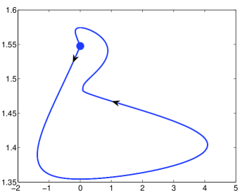
c)
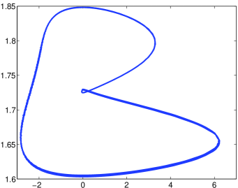
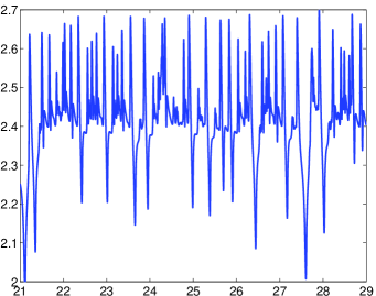
d)

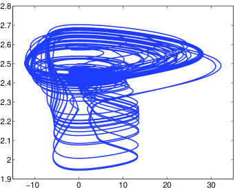
Figure 10: (Color online) Time evolution and phase diagram for the average electric current: a) $\Delta V=31$; b) $\Delta V=33$; c) $\Delta V=35$, d) $\Delta V=40$. For all the calculations $\varkappa=0.1$

With increasing $\Delta V$, $\Delta V>\Delta V_{***}$, $S$ became positive and the contour became unstable. Numerical simulations of (1)–(6) with the white noise initial conditions (8) confirmed the birth of a stable cycle. This is illustrated in Fig. 10(c) where it is shown that the limiting solution acquired periodic oscillations in time. With a further very small increase of $\Delta V$, by about 2% of $\Delta V_{*}$, the limit cycle lost its stability and the oscillations became aperiodic and chaotic, see Fig. 10(d). In this research we did not investigate the details of the transition from periodic to chaotic motion.

With larger $\Delta V$, the oscillations looked much more chaotic, for the behavior in the phase space see Fig. 10(d). The spikes of the space charge not only coalesced aperiodically but their coalescence became very disordered and provided high speed outflow jets upwards (see Fig. 6(c)).

IV.5 Spatial spectra

A spatial Fourier transform of the electric current $j(x)$,

$$F(k)=\left|\int_{0}^{\infty}je^{-ikx}dx\right|,$$ (39)

gives the characteristic size and characteristic wave number of the vortex at any instant of time, $t>0$. In Fig. 11(a), the evolution of $F(k)$ within the interval $\Delta V_{*}<\Delta V<\Delta V_{**}$ is shown. The small-amplitude initial white noise ($t=3\times 10^{-5}$) after filtering by the linear instability evolves into a narrow primary band with a characteristic wave number $k\approx 13$ ($t=1.4\times 10^{-1}$. Beyond this time, however, nonlinearity corrupts this spectrum and wave coalescence makes the characteristic wave length longer, with eventual wave number $k_{D}\approx 5$.

In Fig. 11(b), the typical spectrum evolution for the chaotic regime is presented. After the linear filtering, at $t=9\times 10^{-3}$, overtone and subharmonic bands appear. At the final stage of evolution, the perturbations again acquire coherency, now due to nonlinearity, the characteristic wave number $k_{D}\approx 5$ but it is not steady and it oscillates in time within a narrow frequency window (dashed line) and its Fourier distribution has a pronounced high-frequency band which is also oscillating.

(a)	(b)

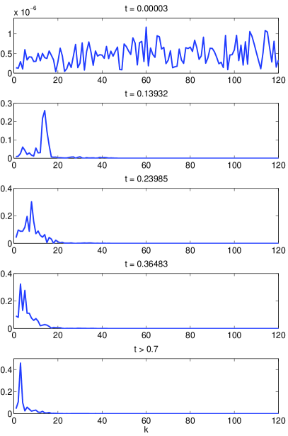
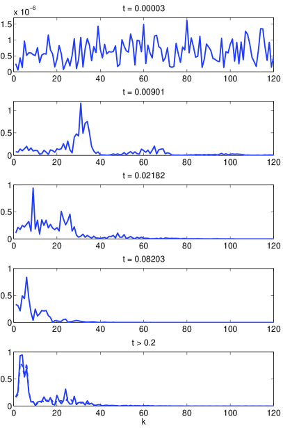
Figure 11: (Color online) Evolution of the spatial Fourier transform $F(k)$, $\varkappa=0.1$ (a) $\Delta V=30$ and (b) $\Delta V=50$

For all our calculations, the typical characteristic wave number of the attractor is within the interval $k_{D}=3\div 5$. It is close to the critical wave number of the instability threshold $k_{*}$, see Table 1. The typical length of the attractor pattern is a multiple of from 1.25 to 2 of the distance between the membranes, $\tilde{L}$.

Table 3: Dominant wave number for $\nu=10^{-3}$ and (a) $\varkappa=0.2$; (b) $\varkappa=0.1$; (c) $\varkappa=0.05$

(a)
$\Delta V$	$k_{D}$
28	5.0
30	4.0
32	3.0
35	3.0
36	3.0
37	4.0
38	5.0
39	5.0
40	4.0
50	4.0

(b)
$\Delta V$	$k_{D}$
32	5.0
33	4.0
33.5	4.0
34	4.0
34.7	3.0
34.8	3.0
35	3.0
37	3.0
40	3.0
50	4.0

(c)
$\Delta V$	$k_{D}$
40	4.0
42	4.0
44	3.0
46	3.0
48	2.0
50	2.0
52	2.0
54	4.0
56	4.0
60	4.0

The simulations were done for the doubled interval, $k=0.5$; the spectrum did not change. The behavior for different $\varkappa$ is qualitatively identical but with increasing $\varkappa$ the solution becomes more chaotic. The dominant wave numbers for $\nu=10^{-3}$ and different $\varkappa$ are presented in Table 3.

IV.6 Comparison with experiment

Electrokinetic instability is a new type of electro-hydrodynamic instability for which experimental evidence was presented only recently (Belv ; RubRub1 ; YCh ; KmHn ). Direct quantitative comparison with experimental data is complicated by many reasons, maybe the main reason is that it is difficult to take into account all the experimental factors involved. Still we will try to evaluate the experimental and theoretical data.

Only the paper Belv contains time series of variables (chronopotentiometric curves) and, in qualitative agreement with our simulations, experimental time series do not show regular periodic oscillations, sinusoidal or close to sinusoidal: there is no evidence of Hopf bifurcation in experiments.

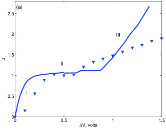
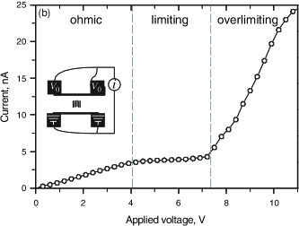
Figure 12: (Color online) (a) VC characteristics for $\kappa=0.05$ and $\nu=10^{-3}$; I, II and III stand for underlimiting, limiting and overlimiting currents, respectively; the triangles corresponds to experiments RubRub1 and the solid line corresponds to our simulations. (b) Experimental data from KmHn clearly shows the regions of underlimiting, limiting and overlimiting currents

From the Table 3, taking into account $\varkappa=0.05$ and $\tilde{L}=0.5$ mm, the dimensional dominant wave number changes within the window $\tilde{k}_{D}=4\div 8\text{ mm}^{-1}$. This is in qualitative agreement with $\tilde{k}_{D}=2\text{ mm}^{-1}$ in RubRub1 . The experimental threshold of instability according to RubRub1 $\Delta\tilde{V}_{*}=0.5$ V, and the theoretical one is (see Table 1) $\Delta\tilde{V}_{*}=0.95$ V.

The experimental RubRub1 and calculated VC characteristics are presented in Fig. 12(a); again they show a qualitative agreement between the theoretical and experimental data. The experimental VC behavior obtained in KmHn qualitatively fits the theoretical one in Fig. 4 (relatively long region of the limiting currents, rather steep VC-dependence for the overlimiting region in comparison with the ohmic region). Unfortunately, many important experimental parameters which are necessary for the comparison are not presented in KmHn .

The final resumé is: there is a qualitative agreement between the theoretical and experimental data. For better quantitative comparison, additional factors must be taken into account.

V Conclusions

The results of direct numerical simulation of electrokinetic instability, described by the system of the Nernst-Planck-Poisson-Stokes equations, were presented. Two kinds of initial conditions were applied: (a) white noise initial conditions were taken to mimic “room disturbances” and the subsequent natural evolution of the solution; (b) an artificial monochromatic ion distribution with a fixed wave number was used to create steady coherent structures.

The results were discussed and understood from the viewpoint of bifurcation theory and the theory of hydrodynamic instability. The following sequence of attractors and bifurcations was observed as the drop of potential between the selective surfaces increased: stationary point — homoclinic contour — limit cycle — chaotic motion; this sequence does not include Hopf bifurcation.

The threshold of electroconvective movement, $\Delta V=\Delta V_{*}$, and the origin of electroconvective vortices were found by the linear spectral stability theory which results were confirmed by the numerical simulation of the Nernst-Planck-Poisson-Stokes system. For a small supercriticality the electroconvective vortices and their stability were described by a weakly nonlinear theory. Direct numerical integration of the entire system extended the results of the weakly nonlinear analysis to finite supercriticality. In particular, a “balloon” of stability of steady vortices was found: $\Delta V_{*}<\Delta V<\Delta V_{**}$. For a large enough drop of potential, $\Delta V>\Delta V_{**}$, all the steady vortices become unstable via real eigenvalues. The new attractor is characterized by aperiodic oscillations when the solution for a long time looks like a steady 2D electroconvective vortex, but eventually the neighboring spikes of the space charge either rapidly coalesce or disintegrate to return to the electoconvective quasi-steady structure. Such a scenario repeats itself many times, forming in the proper phase space a so called stable homoclinic contour.

With further increase of $\Delta V>\Delta V_{***}$, the homoclinic contour loses its stability and the motion first becomes periodic and then, with a very small further increase of $\Delta V$, chaotic. Numerical resolution of the thin concentration polarization layer showed spike-like charge profiles along the membrane surface. For a large enough potential drop, the coalescence of the spikes of the space charge became very disordered and provided high-speed outflow jets and the additional ion flux was dominated by these outflow jets.

The numerical investigation confirms the absence of regular, close to sinusoidal, oscillations for overlimiting regimes. There is a qualitative agreement between the experimental and theoretical thresholds of instability, dominant wave numbers of the observed coherent structures, and voltage–current characteristics.

- (1) B. M. Grafov and A. A. Chernenko, “The theory of the passage of a constant current through a solution of a binary electrolyte,” [in Russian] Dokl. Akad. Nauk SSSR 146, 135 (1962).
- (2) W. H. Smyrl and J. Newman, “Double layer structure at the limiting current,” Trans. Faraday Soc. 63, 207 (1967).
- (3) S. S. Dukhin and B. V. Derjagin, Electrophoresis, 2nd edn. [in Russian] Nauka, Moscow, 1976.
- (4) I. Rubinstein and L. Shtilman, “Voltage against current curves of cation exchange membranes,” J. Chem. Soc. Faraday Trans. II 75, 231 (1979).
- (5) R. P. Buck, “Steady state space charge effects in symmetric cells with concentration polarized electrodes,” J. Electroanal. Chem. Interf. Electrochem. 46, 1 (1973).
- (6) V. V. Nikonenko, V. I. Zabolotsky and N. P. Gnusin, “Electric transport of ions through diffusion layers with impaired electroneutrality,” Sov. Elektrochem. 25, 301 (1989).
- (7) A. V. Listovnichy, “Passage of currents higher than the limiting one through the electrode–electolyte solution system,” Sov. Electrochem. 51, 1651 (1989).
- (8) J. A. Manzanares, W. D. Murphy, S. Mafe and H. Reiss, “Numerical simulation of the nonequilibrium diffuse double layer in ion-exchange membranes,” J. Phys. Chem. 97, 8524 (1993).
- (9) V. A. Babeshko, V. I. Zabolotsky, N. M. Korzhenko, R. R. Seidov, and M. A. Kh. Urtenov, “The theory of steady-state transport of a binary electrolyte in the one-dimensional case,” [in Russian] Dokl. Akad. Nauk 361, 41 (1998).
- (10) K. T. Chu and M. Z. Bazant, “Electrochemical thin films at and above the classical limiting current,” SIAM J. Appl. Math. 65, 1485 (2005).
- (11) I. Rubinstein and B. Zaltzman, “Electro-osmotically induced convection at a permselective membrane,” Phys. Rev. E 62, 2238 (2000).
- (12) I. Rubinstein and B. Zaltzman, “Wave number selection in a nonequilibrium electroosmotic instability,” Phys. Rev. E 68, 032501 (2003).
- (13) I. Rubinstein, E. Staude, and O. Kedem, “Role of the membrane surface in concentration polarization at ion-exchange membrane,” Desalination 69, 101 (1988).
- (14) F. Maletzki, H. W. Rossler, and E. Staude, “Ion transfer across electrodialysis membranes in the overlimiting current range: Stationary voltage–current characteristics and current nouse power spectra under different condition of free convection,” J. Membr. Sci. 71, 105 (1992).
- (15) E. I. Belova, G. Y. Lopatkova, N. D. Pismenskaya, V. V. Nikonenko, C. Larchet, and G. Pourcelly, “Effect of anion-exchange membrane surface properties on mechanisms of overlimiting mass transfer,” J. Phys. Chem. B 110, 13458 (2006).
- (16) I. Rubinstein, B. Zaltzman, J. Pretz, and C. Linder, “Experimental verification of the electroosmotic mechanism of overlimiting conductance through a cation exchange electrodialysis membrane,” Rus. J. Electrochem. 38, 853 (2004).
- (17) S. M. Rubinstein, G. Manukyan, A. Staicu, I. Rubinsten, B. Zaltzman, R. G. H. Lammertink, F. Mugele and M. Wessling, “Direct observation of nonequilibrium electroosmotic instability,” Phys. Rev. Lett. 101, 236101 (2008).
- (18) G. Yossifon and H.-C. Chang, “Selection of nonequilibrium overlimiting currents: Universal depletion layer formation dynamics and vortex instability,” Phys. Rev. Lett. 101, 254501 (2008).
- (19) S. J. Kim, Y.-C. Wang, J. H. Lee, H. Jang and J. Han, “Concentration polarization and nonlinear electrokinetic flow near a nanofluidic channel,” Phys. Rev. Lett. 99, 044501.1 (2007).
- (20) B. Zaltzman and I. Rubinstein, “Electroosmotic slip and electroconvective instability,” J. Fluid Mech. 579, 173 (2007).
- (21) E. A. Demekhin, V. S. Shelistov and S. V. Polyanskikh, “Linear and nonlinear evolution and diffusion layer selection in electrokinetic instability,” Phys. Rev. E 84, 036318 (2011).
- (22) H.-C. Chang, E. A. Demekhin, and V. S. Shelistov “Competition between Dukhin’s and Rubinstein’s electrokinetic modes,” Phys. Rev. E 86, 046319 (2012).
- (23) V. S. Pham, Z. Li, K. M. Lim, J. K. White, and J. Han, “Direct numerical simulation of electroconvective instability and hysteretic current-voltage response of a permselective membrane,” Phys. Rev. E 86, 046310 (2012).
- (24) E. N. Kalaidin, S. V. Polyanskikh, and E. A. Demekhin, “Self-similar solutions in ion-exchange membranes and their stability,” Doklady Physics 55, 502 (2010).
- (25) E. A. Demekhin, S. V. Polyanskikh and Y. M. Shtemler, “Electroconvective instability of self-similar equilibria,” e-print arXiv: 1001.4502.
- (26) E. A. Demekhin, E. M. Shapar, and V. V. Lapchenko, “Initiation of electroconvection in semipermeable electric membranes,” Doklady Physics 53, 450 (2008).
- (27) V. Nikonenko, N. Pismenskaya, E. Belova, P. Sistat, P. Huguet, G Pourcelly and C. Larchet, “Intensive current transfer in membrane systems: Modelling, mechanisms and application in electrodialysis,” Advances in Colloid and Interface Science 160, 101 (2010).
- (28) T. Pundik, I. Rubinstein and B. Zaltzman, “Bulk electroconvection in electrolyte,” Phys. Rev. E 72, 061502 (2005).
- (29) N. Nikitin, “Third-order-accurate semi-implicit Runge-Kutta scheme for incompressible Navier-Stokes equations,” Int. J. Num. Meth. Fluids 51, 2, 221, (2005).
- (30) N. Nikitin, “ Finite-difference method for incompressible Navier-Stokes equations in arbitrary orthogonal curvilinear coordinates,” J. Comput. Phys. 217, 2, 759, (2006).
- (31) N. V. Nikitin, “On the rate of spatial predictability in near-wall flows,” J. Fluid Mech. 614, 495 (2008).
- (32) N. V. Nikitin, “A spectral finite-difference method of calculating turbulent flows of an incompressible fluid in pipes and channels,” Computational Mathematics and Mathematical Physics 34, 785, (1994).
- (33) N. V. Nikitin. “Statistical characteristics of wall turbulence,” Fluid Dynamics 31 361 (1996).
- (34) M. C. Cross and P. G. Hohenberg, “Pattern formation outside of equilibrium,” Rev. Modern Physics 65, 3, 851 (1993).
- (35) W. Eckhaus, Studies in nonlinear stability theory, Springer-Verlag, 1965.
- (36) H.-C. Chang, E. A. Demekhin, and D. I. Kopevevich “Nonlinear evolution of waves on a vertically falling film,” J. Fluid Mech. 250, 443 (1993).
- (37) J. Guckenheimer and P. Holmes, Nonlinear oscillations, dynamical system and bifurcations of vector fields, Springer-Verlag, 1983.