Evolution of a family of expanding cubic black-hole lattices in numerical relativity

Abstract

We present the numerical evolution of a family of conformally-flat, infinite, expanding cubic black-hole lattices. We solve for the initial data using an initial-data prescription presented recently, along with a new multigrid solver developed for this purpose. We then apply the standard tools of numerical relativity to calculate the time development of this initial dataset and derive quantities of cosmological relevance, such as the scaling of proper lengths. Similarly to the case of $S^{3}$ lattices, we find that the length scaling remains close to the analytical solution for Friedmann-Lemaître-Robertson-Walker cosmologies throughout our simulations, which span a window of about one order of magnitude in the growth of the scale factor. We highlight, however, a number of important departures from the Friedmann-Lemaître-Robertson-Walker class.

1 Introduction

Black-hole lattices have recently attracted some attention as simple models of a universe in which inhomogeneities coexist with a large-scale symmetry represented by an exact, discrete invariance under rigid translations taking each black hole into one of its neighbours  [1, 2, 3, 4, 5, 6, 7, 8]. They serve as relatively simple test beds to study whether small scale inhomogeneities can influence the large scale behavior of the model in a significant way and produce various backreaction effects [9]. Despite their lack of Killing vectors, they retain a discrete group of isometries and thus remain homogeneous on large scales.

Initial data for both contracting [2, 4, 7] and expanding [5] lattices have appeared in the literature, along with the analysis of their properties, such as the mass-to-expansion-rate proportionality and the associated backreaction problem. In the case of lattices which are momentarily at rest, the full numerical-relativity evolution of the 8-black-hole model has been carried out for roughly one half of the collapsing time of the corresponding Friedmann-Lemaître-Robertson-Walker (FLRW) spacetime, exhibiting a length scaling that remained close to the FLRW counterpart at essentially all times [7].

In this work, we build on [7] and apply the same analysis to the evolution of initial data for an expanding cubic lattice, which we construct using the prescription from [5]. We then compare the result with its natural homogeneous counterpart, i.e. flat FLRW model with dust.

The paper is organized as follows: in the next section we discuss the numerical construction of the initial data. In section 3 we discuss the results of the initial data construction and the numerical evolution. In section 4 we compare the results with the corresponding FLRW universe, and draw our conclusions in section 5. A number of details, such as the convergence study and the gauge conditions necessary to evolve black holes in an expanding lattice, are discussed in the appendices.

2 Constructing initial data for a periodic, expanding black-hole lattice

In order to solve for initial data, we start with the standard 3+1 decomposition of the metric tensor, where one works with the spatial metric $\gamma_{ij}$ and extrinsic curvature $K_{ij}$. In these terms, the Einstein constraints take the form:

$$R+K^{2}-K_{ij}K^{ij}=0$$ (1)

$$D_{j}K^{j}_{i}-D_{i}K=0$$ (2)

In [5], an expanding lattice solution is presented where the trace of the extrinsic curvature $K_{ij}$ on the initial slice transitions from zero near the center to a constant, negative value next to the periodic faces. One can thus expect to recover the Schwarzschild solution in the familiar isotropic coordinates next to the black holes, whilst the volume expansion of the cell faces, represented (up to a sign) by the trace of the extrinsic curvature, is constant and positive, thus mimicking a homogeneous and isotropic spacetime, at least initially.

We generate similar initial data, following some of the prescriptions of [5], in [10]. The results are obtained by solving the constraints equation according to the Lichnerowicz-York scheme:

$$\tilde{\Delta}\psi-\frac{\tilde{R}}{8}\,\psi-\frac{K^{2}}{12}\,\psi^{5}+\frac{1}{8}{\tilde{A}}_{ij}{\tilde{A}}^{ij}\psi^{-7}=0$$ (3)

$$\tilde{D}_{i}\tilde{A}^{ij}-\frac{2}{3}\psi^{6}\tilde{\gamma}^{ij}\tilde{D}_{i}K=0$$ (4)

We choose a flat metric as the conformal “background” metric:

$$\tilde{\gamma}_{ij}=\delta_{ij}$$ (5)

$$\tilde{R}=0$$ (6)

and the following form for the traceless part of the extrinsic curvature:

$$\tilde{A}_{ij}=\tilde{D}_{i}X_{j}+\tilde{D}_{j}X_{i}-\frac{2}{3}\tilde{\gamma}_{ij}\tilde{D}_{k}X^{k}$$ (7)

$X_{i}$ being a new variable to solve for. The trace of the extrinsic curvature takes the form

$$K=K_{c}W$$ (8)

where $W$ is a function that vanishes near the center and is equal to one on the faces, with a smooth transition region in between:

$$W(r) = \left\{\begin{array}[]{ll}0&\textrm{for }0\leq r\leq l\\ \left(\frac{(r-l-\sigma)^{6}}{\sigma^{6}}-1\right)^{6}&\textrm{for }l\leq r\leq l+\sigma\\ 1&\textrm{for }l+\sigma\leq r\end{array}\right.$$ (12)

with $0\leq l\leq l+\sigma\leq L$ (see equation (13) in [5]). The conformal factor is further decomposed in its singular part, with a simple $m/r$ behaviour, and a regular part $\psi_{r}$ which is solved for:

$$\psi=\psi_{r}+\frac{m}{2r}\left(1-W(r)\right)$$ (13)

Notice that a non-constant $K$ implies that the full coupled system of Hamiltonian and momentum constraints [11, 12] has to be solved concurrently. This is one of the main differences with the work in [7]. The resulting system reads (dropping all the tildes as now all quantities refer to the flat, conformal metric):

$$\Delta\psi_{r}-\Delta\left(\frac{m}{2r}W(r)\right)-\frac{K^{2}}{12}\,\psi^{5}+\frac{1}{8}{A}_{ij}{A}^{ij}\psi^{-7}=0$$ (14)

$$\Delta X^{i}+\frac{1}{3}\partial^{i}\partial_{j}X^{j}-\frac{2}{3}\psi^{6}\partial^{i}K=0$$ (15)

In [5], periodic boundary conditions are imposed on $\psi_{r}$. Notice that $X^{i}$ needs not be periodic in order to have a periodic $\tilde{A}_{ij}$. However, we have found that imposing periodic boundary conditions on $X^{i}$ does not affect the generality of the solution; therefore, we impose periodic boundary conditions on all the variables of our system. Furthermore, in [5] the divergence of $X^{i}$ is introduced as an auxiliary variable named $Z=\partial_{i}X^{i}$. We have found no particular benefit in this choice; as a matter of fact, we have found that solving the new system with relaxation leads to rather large violations of the constraint $Z=\partial_{i}X^{i}$, which slow down convergence unless the constraint is enforced after every step.

All the quantities in the problem have to be such that the integrability condition is satisfied:

$$K_{c}^{2}\int W^{2}\psi^{5}=2\pi\left(m+\frac{1}{8}\int\tilde{A}_{ij}\tilde{A}^{ij}\psi^{-7}\right)$$ (16)

As explained in [10], one only has to worry about the condition associated to the Hamiltonian constraint as the one for momentum constraint is satisfied identically. In [5], this condition is satisfied by solving $K_{c}$. In [10], however, we find that fixing $K_{c}$ at the start and tuning the zero-frequency part of $\psi$ leads to faster convergence of the relaxation algorithm (this comes at the price of introducing a root-finding step at the end of each relaxation step, and also of giving up control of the scale of $\psi$ at the origin, which is directly related to the ADM mass of the black hole, as will be shown below). This is what we ultimately use to generate the initial data evolved in this paper. We also perform the resetting:

$$X^{i}\to X^{i}-X^{i}(O)$$ (17)

to fix the zero mode of $X^{i}$, not determined by the periodic linear equation.

As opposed to [7], we have three free parameters to specify in this class of solutions: the mass parameter of each black hole $m$, the coordinate semilength $L$ of the lattice edge, and the value of $K_{c}$. Physically, however, they are not entirely independent because the equations are invariant under the rescaling $m\to\lambda\,m$, $L\to\lambda\,L$ and $K_{c}\to\lambda^{-1}K_{c}$. Therefore we will parametrize our solution by a single scale–invariant number instead of the bare mass $m$. The parameter $\mu$, representing the degree of lumpiness of the solution, can e.g. be defined as:

$$\mu=\frac{m_{\rm BH}(m,L,K_{c})}{D_{\rm edge}(m,L,K_{c})}$$ (18)

where $m_{\rm BH}$ is the ADM mass of the black hole, and $D_{\rm edge}$ is the initial proper length of a cell’s edge.

3 Results

In order to solve for the initial data of a black hole in a cubic cell with periodic boundaries enforced at the faces, we apply the multigrid elliptic solver described in [10]. This code is designed to be used with the infrastructure of the Einstein Toolkit [13]; in particular, it is implemented as a module for the Cactus framework and relies on the Carpet AMR package [14].

The multigrid implementation is rather standard: on each refinement level, the constraint system or the associated error equation is smoothed using a non-linear Gauss-Seidel solver, and information is passed between levels through the Carpet restriction and prolongation operators, and following the Full Approximation Scheme (FAS). The levels are traversed according to Full Multigrid (FMG) prescription. We refer to [10] for the details.

Once the initial data are generated, we evolve them using the Einstein evolution code McLachlan. The evolution and analysis tools used here are almost identical to those presented in [7]: we use the same BSSN formulation of the Einstein evolution system, but we slightly modify the usual moving-puncture gauge to prevent the exponential increase of the lapse in regions with negative $K$ (see B). In order to carry out the coordinate transformation from numerical to proper time, we use the same strategy and tools described in [7].

The grid setup involves a base grid extending to $x=\pm 5$, $y=\pm 5$ and $z=\pm 5$, with spacing $\Delta_{0}=1$ and with four additional grids covering the same domain, each at double the spatial resolution as the previous one, so that the finest resolution at the center is given by $\Delta_{4}=0.0625$. In the $m=1$ case, we also run two additional resolutions, with $\Delta_{0}=5/6$ and $\Delta_{0}=5/8$, in order to quantify the numerical error.

Unlike regular lattices on $S^{3}$, in a regular lattice on a flat background we have the freedom to vary the density parameter continuously. We choose four values of $m={0.5,1,2,5}$ and set $K_{c}=-0.21$, obtaining the ADM masses and initial proper cell-edge lengths in Table 1.

Table 1: Initial data parameters for the four runs with $m={0.5,1,2,5}$ and $K_{c}=-0.21$. $m_{\rm BH}$ is the ADM mass of the black hole at the center, and $|H|$ the $L_{2}$-norm of the Hamiltonian constraint. For the $m=1$ configuration, three resolutions $\Delta_{0}={5/8,5/6,1}$ have been run to quantify the numerical error.

Run	$m$	$m_{\rm BH}$	$D_{\rm edge}(t=0)$	$|H|$	$\Delta_{0}$
L1	1	1.00797	12.2607	$1.29\cdot 10^{-4}$	1
L2	1	1.00800	12.2607	$7.03\cdot 10^{-5}$	5/6
L3	1	1.00801	12.2604	$2.72\cdot 10^{-5}$	5/8
L4	0.5	0.46060	9.41388	$1.61\cdot 10^{-3}$	1
L5	2	2.13032	15.9943	$2.36\cdot 10^{-5}$	1
L6	5	6.34535	26.9543	$8.99\cdot 10^{-4}$	1

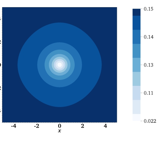
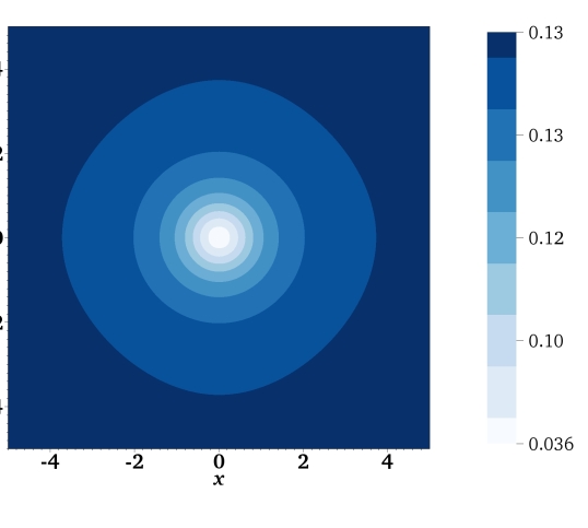
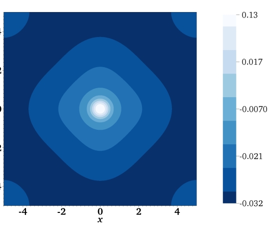
The evolution of the conformal factor $W=\psi^{-2}$ is rather featureless, with an overall change in scale as the most prominent effect. Profiles of $W$ at $t=0,30,60,90,120$ and $150$ are displayed in Figure 1.

Figure 1: Profiles of $W=\psi^{-2}$ on the equatorial plane at $t=0,30,60,90,120$ and $150$ for the $m=1$, $\Delta_{0}=1$ run.

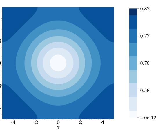
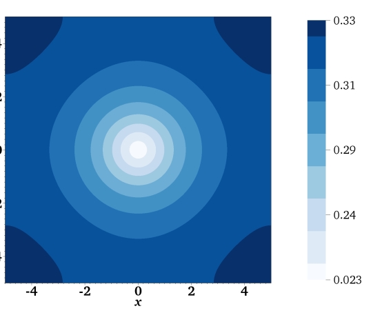
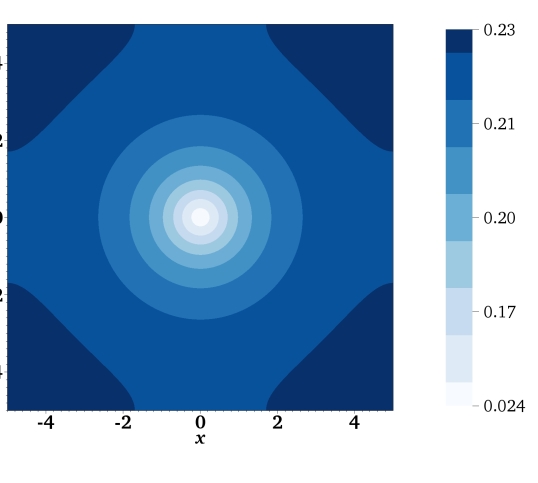
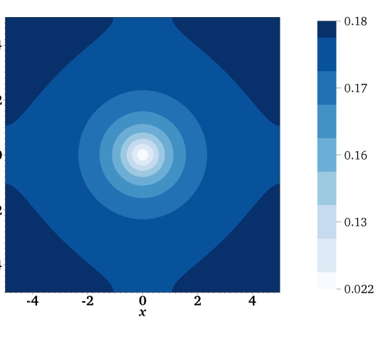
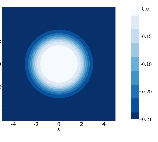
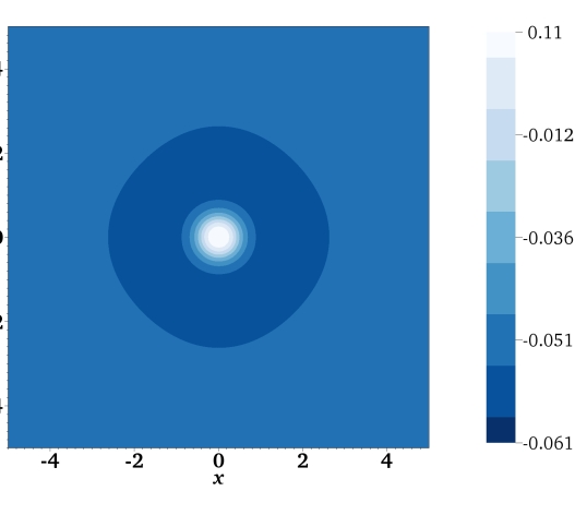
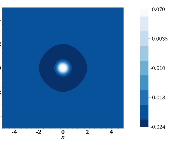
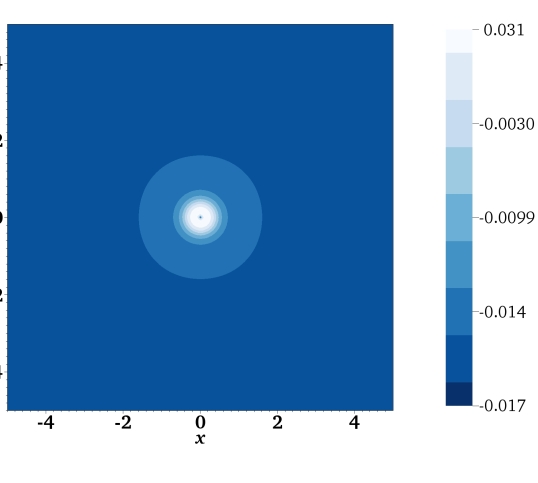
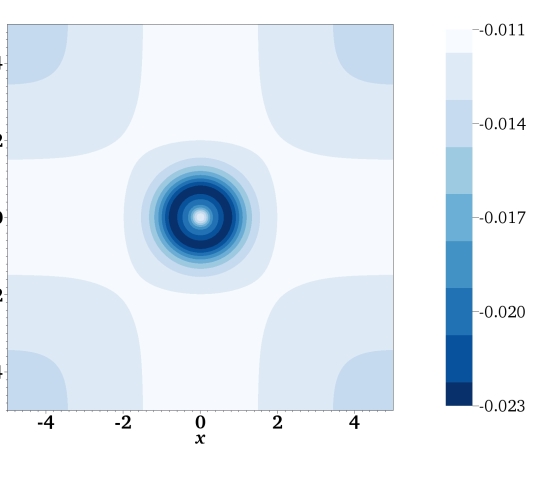
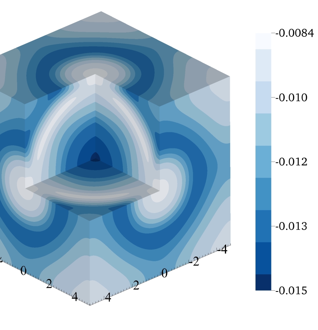
The trace of the extrinsic curvature $K$, on the other hand, transitions from a nearly-spherically-symmetric initial profile, with zero $K$ at the center, to a configuration where $K$ is negative everywhere, with a maximum in magnitude on the faces and a minimum at the center (see Figures 2 and  3). There is also an overall change in scale corresponding to that observed in $W$.

Figure 2: Profiles of $K$ on the equatorial plane at $t=0,30,60,90,120$ and $150$ for the $m=1$, $\Delta_{0}=1$ run.

Figure 3: The mean curvature $K$ at time $t=180$ for the $m=1$, $\Delta_{0}=1$ run. The $z$-axis runs vertically.

The $L_{2}$ norm of the Hamiltonian constraint and the $x$-component of the momentum constraint are shown in Figure 4 for L1, L2 and L3, the three resolutions of the $m=1$ case. Two-dimensional, equatorial sections of the Hamiltonian constraint for L1 are shown in Figure 5: this shows that the violations do not significantly grow in time, remaining, outside the apparent horizon, always lower than $10^{-2}$. The constraint violations, however, only converge to zero for $t<70$; the Hamiltonian constraint converges at fourth order first, and eventually at first order; the convergence order of the momentum constraint is much less clear.

Figure 4: $L_{2}$ norms of the Hamiltonian and momentum constraint for runs L1, L2 and L3. The constraint violations only converge to zero for $t<70$.

Figure 5: Profiles of $|H|$ on the equatorial plane at $t=0,30,60,90,120$ and $150$ for the $m=1$, $\Delta_{0}=1$ run.

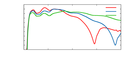
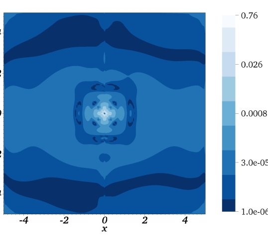
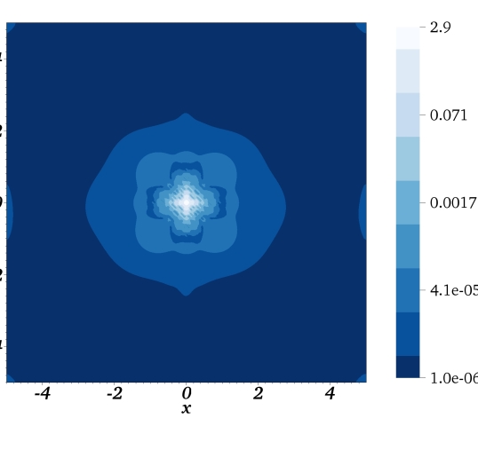
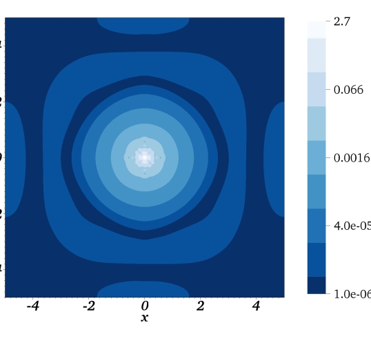
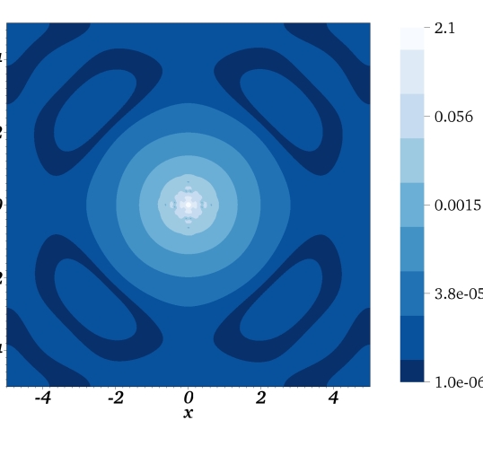
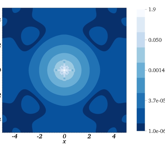
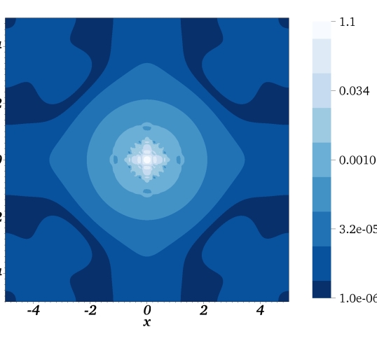
These quantities, like a number of others below, show considerable oscillations throughout the evolution. This is not surprising as, due to the periodic boundaries, travelling modes will not be able to disperse at infinity, but will rather be trapped inside the domain and keep interfering with themselves. If the result acquires a high-frequency component, due to the large truncation error the constraints may increase accordingly. This effect would decrease if we increased the resolution – as do some of the features in Figure 4.

It is interesting to ask where these modes could originate. An obvious culprit is the assumption of conformal flatness that underlies our initial-data construction; a similar connection exists in the conformally-flat initial data for binary black-hole systems in asymptotically-flat spaces, which are known to contain spurious gravitational radiation that travels out from the binary region right at the beginning of the evolution. Whilst defining gravitational waves in our setting is not as straightforward, it is conceivable that a similar mechanism is at play here, and that the assumption of conformal flatness sets up the lattice in a state which is mixed with oscillatory modes.

4 Comparison with the FLRW class

In this section we will compare the results with the FLRW class of solutions with dust and evaluate all possible discrepancies, called in this context the cosmological backreaction. We focus on three aspects: the scaling of proper lengths, and the cell’s effective mass and pressure which can be defined via the first and second Friedmann equations respectively.

We will examine these three quantities in the following subsections. For the purpose of this paper we will divide the backreaction effects into kinematical, i.e. those that can be read out directly from the initial data, and dynamical, which appear as we evolve the data in time. It turns out that the kinematical backreaction effects can be interpreted as a “dressing” of the bare black hole masses while the dynamical ones can be thought of as an additional effective-pressure term in the Friedmann equations.

In addition to a comparison with homogeneous cosmologies, the analysis highlights some of the technical issues arising in the simulation of lattices with too high, or too low, a ratio of mass to cell size. As this ratio grows, so does the ratio of the apparent horizon radius to the cell linear size $L$; this leaves less and less room for the transition between the Schwarzschild solution at the center and the constant-mean-curvature (CMC) region at the edges. Correspondingly, it is harder and harder to reduce the constraint violations in the initial data: as illustrated in Table 1, the $L_{2}$-norm of the Hamiltonian constraint violation for $m=5$ is almost an order of magnitude larger than for $m=1$. At the opposite end of the spectrum, smaller values of the mass-to-size ratio require correspondingly finer grids in order to resolve the central black hole; decreasing this ratio at constant resolution leads to a length scaling that tends to a linear law – the length scaling of empty space in a CMC foliation.

4.1 Proper length of a cell edge

A comparison with the homogeneous Friedmann-Lemaître-Robertson-Walker class with dust requires solving Ellis’s fitting problem, i.e. finding the FLRW model which resembles each black-hole lattice most closely.

In this paper we will follow the approach from [7], also similar in spirit to [4]. Consider the edges of lattice cells at $t=0$: obviously they constitute identical geodesic segments, each meeting five others at right angles at each vertex. While the lattice faces are not isometric to flat squares, the edges still constitute a regular lattice which is entirely isometric to a cubic lattice of edge length $D_{\rm edge}(0)$ in flat space. Due to the discrete symmetry of the initial data this property carries over to all times provided that the shift function preserves all the symmetries. We will assume for the purpose of the FLRW fitting that the gauge is such that $\alpha=1$ and $\beta^{i}=0$. This requires of course a numerical refoliation of at least a part of the spacetime.

Clearly, an arrangement of cells with edges isometric to a cubic lattice can only be found in a flat FLRW model. Thus we will take a flat FLRW as our reference model: we fix a flat, three–dimensional space with metric $\delta_{ij}$ containing a cubic lattice of length $D_{\rm edge}(0)$. In order to single out exactly one flat dust FLRW model, we also need to set the Hubble parameter at $t=0$, which we fix to $\dot{D}_{\rm edge}(0)/D_{\rm edge}(0)$. We label these models with FLRW($m$).

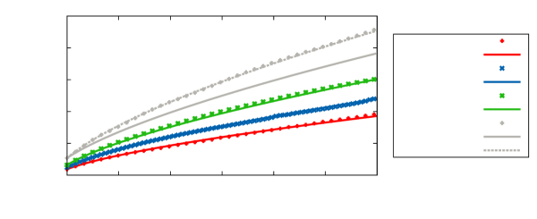
As in [7], given the spatial metric, the lapse and the shift on an edge, we can calculate the expansion of its proper length as a function of proper time. The result is shown in Figure 6 for the four models considered here, for the edge at $x=5$ (the others differ for less than $10^{-3}$ for $m=1$) and with error bars deriving from the error analysis (see A). In the same plot, we show the length scaling of the corresponding FLRW universes defined above, through the fitting of the initial edge length and its first derivative. The length of the black-hole lattice edges remains close to that of the FLRW counterpart at all times, except for the $m=5$ case, where the value of $\dot{D}_{\rm edge}(0)$ does not seem to single out a well-fitting FLRW model; we attribute this to the fact that, for $m=5$, $D_{\rm edge}(t)$ presents high-amplitude oscillations on top of the leading-order length expansion, so that the value of its tangent at a single point may be rather different from the “average” expansion rate. Choosing a different FLRW counterpart, such as the one with initial density equal to $m_{\rm BH}/D^{3}_{\rm edge}(0)$ (labelled FLRWb(5)), improves the fit.

Figure 6: Scaling of the edge proper length as a function of proper time, for $m={0.5,1,2,5}$.

As we were preparing this manuscript, a paper appeared [15] in which the authors address the same issue of proper-length scaling in an expanding black-hole lattice. There, however, the FLRW counterpart is chosen by a parameter fit of the evolution data. Given the evidence in this section, it turns out that this is unnecessary: choosing the mapping based on the kinematical properties of the initial data alone automatically leads to a well-fitting expansion at subsequent times.

4.2 Effective mass

We begin by introducing a dimensionless inhomogeneity parameter:

$$\mu=\frac{m_{\rm BH}}{D_{\rm edge}(0)}$$ (19)

measuring the lumpiness of a given mass distribution. Here $m_{\rm BH}$ denotes the ADM mass of the black hole evaluated at the asymptoticaly flat region near $r=0$. This mass is related to the bare mass parameter by $m_{\rm BH}=m\,\psi_{r}(0)$. This is easy to see if we transform to spherical coordinates $(r,\theta,\varphi)$ and then change the radial coordinate to $\hat{r}=\frac{m^{2}}{4r}$. In the new coordinates the asymptoticaly flat region of the black hole corresponds to $\hat{r}\to\infty$ and the metric takes again a conformally-flat form with the conformal factor $\hat{\psi}=1+\frac{m\psi_{r}}{2\hat{r}}$. The ADM mass can now be read out from the asymptotic behavior of $\hat{\psi}$ at infinity.

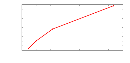
The physical interpretation of $\mu$ as the inhomogeneity parameter is easy to understand if we note that, for a fixed energy density $\rho=m_{\rm BH}/{D^{3}_{\rm edge}}$, we have $\mu=\rho D_{\rm edge}^{2}$ and the parameter decreases as the size of the cell goes to zero. We expect that for a fixed $\rho$ and $\mu$ going to zero the properties of the lumpy model will match those of the homogeneous model. In Figure 7 we plot $\mu$ as a function of the ADM mass of the black hole for four values of the bare mass $m=0.5,1,2,5$, and with $K_{c}=-0.21$. The dependence is not exactly linear because the physical size of the cell $D_{\rm edge}$ depends on the conformal factor $\psi$, which in turn depends on the ADM mass in a non-trivial way.

Figure 7: $\mu$ parameter as a function of the ADM mass of the black hole, for $m={0.5,1,2,5}$.

Note that the procedure outlined above for fitting an FLRW model to the initial data can be repeated at any other time $t$ by an appropriate rescaling of the metric of the FLRW counterpart, such that the proper length of the edge in the FLRW model becomes equal to $D_{\rm edge}(t)$. In this way we obtain a family of “tangent” flat FLRW models parametrized by $t$. Accordingly, we can define a time–dependent effective Hubble parameter to be ${H}_{\rm eff}(t)=\dot{D}_{\rm edge}(t)/D_{\rm edge}(t)$ at any time $t$. We take the effective 3–dimensional Ricci scalar ${R}_{\rm eff}$ of our solution to be equal to the Ricci scalar of the corresponding FLRW, which is of course zero at all times. The first Friedmann equation

$${H}_{\rm eff}^{2}+\frac{{R}_{\rm eff}}{6}=\frac{8\pi}{3}\,{\rho}_{\rm eff}$$ (20)

will now serve as the definition of the effective energy density ${\rho}_{\rm eff}$. In our case it simply reads

$${\rho}_{\rm eff}(t)=\frac{3\dot{D}_{\rm edge}^{2}(t)}{8\pi\,D_{\rm edge}^{2}(t)}.$$ (21)

We may now compare the effective mass enclosed in a single cell, given by ${M}_{\rm eff}={\rho}_{\rm eff}\,D_{\rm edge}(t)^{3}$, with the mass of the black hole as measured is its asymptotically flat end at time $t=0$. This gives the overall mass dressing effect due to the self–interaction of the strong gravitational field. It manifests itself as a difference between the ADM mass, intrinsic to the black hole, and the effective mass contained in a cell as it is “felt” by the Friedmann equations.

Figure 8: Relative mass deficit $x=\frac{M_{\rm eff}-m_{\rm BH}}{M_{\rm eff}}$ as a function of $\mu$, for $m={0.5,1,2,5}$.

Figure 9: Effective mass $M_{\rm eff}$ as a function of proper time, for $m={0.5,1,2,5}$.

In Figure 8, we have plotted the relative mass deficiency parameter $x$, defined as

$$x=\frac{M_{\rm eff}-m_{\rm BH}}{M_{\rm eff}},$$ (22)

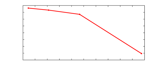
against the values of $\mu$ for the four cases we consider. We have found out that the effective mass is smaller than the ADM mass, unlike the spherical case we investigated in [7]. Rather than the ”gravitating gravity” effect, in which the strong gravitational field contributes positively to the effective mass, we see an effective shielding of the black-hole mass whose magnitude grows nonlinearly with $\mu$.

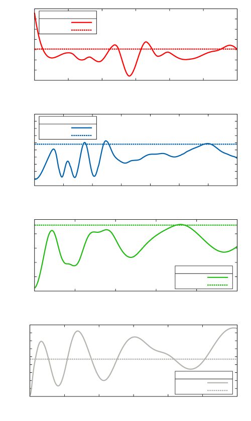
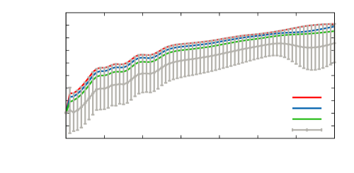
During the evolution, $M_{\rm eff}$ oscillates, sometimes reaching values larger than the ADM mass, as shown in Figure 9. This effect is, for the proper time $\tau<70$, largely independent from the resolution, as indicated by the error bars in Figure 14.

Identifying the origin of this oscillations is not straightforward. Here we will only remark that the initial part is dominated by a single frequency in the range $(0.3-0.5)m_{\rm BH}^{-1}$, i.e. the range of frequencies of the lowest quasi–normal modes of a Schwarzschild black hole.

4.3 Effective pressure

At any time $t$, the reference FLRW spatial slice will have a rescaled metric $D_{\rm edge}(t)^{2}/D_{\rm edge}(0)^{2}\,\delta_{ij}$, so that the size of the lattice edge matches exactly the size of the lattice cell of the inhomogeneous model at $t$.

The second Friedmann equation for the effective parameters, i.e. the evolution equation

$$\frac{\ddot{D}_{\rm edge}}{D_{\rm edge}}=-\frac{4\pi}{3}\left({\rho}_{\rm eff}+3{p}_{\rm eff}\right)$$ (23)

can be used to define an effective pressure $p_{\rm eff}$. After the substitution of (20) and setting ${R}_{\rm eff}$ to zero, it reads

$${p}_{\rm eff}=-\frac{1}{4\pi}\frac{\ddot{D}_{\rm edge}(t)}{D_{\rm edge}(t)}-\frac{1}{8\pi}\frac{\dot{D}_{\rm edge}(t)^{2}}{D_{\rm edge}(t)^{2}}.$$ (24)

If no backreaction effects were present, the pressure would naturally be zero at all times since the black holes do not interact with each other by any means other than gravitational attraction. In Figure 10 we see the effective pressure plotted for $m=1$ and three resolutions in runs L1, L2 and L3. The pressure starts out at zero and oscillates with relatively small amplitude (around $10^{-5}$), and eventually gets damped out to zero. The behavior of $p_{\rm eff}$ is similar for $m=2$, whilst for $m=5$ one observes an initial non-zero effective pressure, again probably due to the same effect discussed in Figure 6. For the largest mass $m=5$, the initial amplitude of the oscillations is around $10^{-4}$.

Since both effective pressure and density appear in equation (23), it is reasonable to compare their influence on the dynamics of the model. It turns out that the amplitude of the oscillations of $p_{\rm eff}$ is somewhat smaller in magnitude than the value of $\rho_{\rm eff}$ for $m=1$ and $m=2$ (the ratio is around 0.3 and 0.15 respectively), although their ratio is close to one in the $m=5$ case. Overall, the evolution of $D_{\rm edge}$, given by (23), is dominated by $\rho_{\rm eff}$ in all cases, because even though the pressure term is comparable with the density term, it is at the same time oscillating rapidly around zero and its influence averages out to zero.

Figure 10: Top: effective pressure for runs L1, L2 and L3 ($m=1$, $\Delta_{0}=1,5/6$ and $5/8$ respectively). Bottom: effective pressure for runs L1, L5 and L6 ($\Delta_{0}=1$, $m=1,2$, and $5$ respectively).

5 Conclusions

We have presented the evolution of a family of cubic black-hole lattices, starting from a conformal transverse-traceless set of initial data proposed by [5] and reproduced by us via a multigrid elliptic solver.

After a description of some of the 3+1 quantities during the evolution, we constructed three observables to use as a ground of comparison between these solutions and some suitably-chosen FLRW counterpart: the proper length of the periodic cell’s edge and its scaling according to geodesic observers, and an effective mass and pressure defined through the first and second Friedmann equations.

We find that, while the scaling remains close to the dust-FLRW law for the evolutions considered here, a number of important differences emerges: first, the study of the $m=1$ case shows that the proper length, extrapolated to infinite numerical resolution, differs from the FLRW law by up to $1.5\%$ for $t<70$; this is over an order of magnitude higher than the numerical error bars. After this time, the numerical convergence becomes less clear and it is impossible to evaluate the agreement.

Second, taking time derivatives of this observable brings out the presence of oscillatory modes superimposed on the zero-frequency behavior. Using an analogy to the similar occurrence in conformal-transverse-traceless initial data for multiple black holes in asymptotically-flat spaces, we conjecture that these vibrations may be due to the somewhat simplified initial data construction. Unlike the asymptotically-flat case, however, these modes cannot diffuse to infinity, and remain present at all times.

The main backreaction effect we observe is the mass dressing, i.e. the difference between the “bare” ADM mass of the central black hole and the effective mass of the individual cell. In the initial data, the effective mass is smaller than the ADM mass in all cases, the effect growing with the inhomogeneity parameter in a nonlinear manner. Furthermore, the effective mass turns out to be time–dependent; its value oscillates during the evolution around values somewhat smaller than the ADM mass. While most of the time it remains smaller than the ADM mass, it can actually get larger for a short time. Analyzing its power spectrum, we find peaks in the band of the quasinormal frequencies of a Schwarzschild black hole of comparable mass. Finally, the effective pressure, whose non–vanishing values are the main dynamical backreaction effect in these models, undergoes similar damped oscillations around the zero value with relatively small amplitude.

We conclude that this set of initial data has a leading-order behavior that remains close to the FLRW model of matching initial energy density, but presents noticeable higher-order oscillations which affect the evolution. Whether it would be feasible to prepare an expanding black-hole lattice in a “purer” initial state remains a question for future studies.

Appendix A Convergence and numerical errors

We performed a three-point convergence test using the proper edge length of run L1, L2 and L3. The convergence factor

$$c\equiv\frac{|D^{(\\ \rm c)}-D^{(\\ \rm m)|}}{|D^{(\\ \rm m)}-D^{(\\ \rm f)}|}$$ (25)

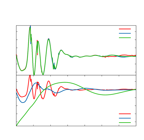
remains close to the first-order value until $t\approx 50$, as illustrated in Figure 11.

Figure 11: Convergence factor from the three-point convergence test.

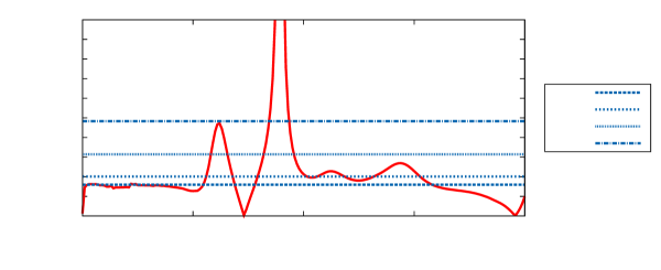
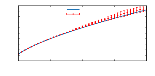
Using this, one can extrapolate to the continuum limit, $\Delta\to 0$, obtaining the curve in Figure 12, with error bars given by the difference between the continuum limit and the coarsest resolution. In Figure 13, the difference between the edge length in L1, L2, L3, and the continuum solution and the scale factor of a FLRW universe with the same initial expansion rate is compared.

Similarly, in Figures 14 and 15, the continuum limit of the effective mass and effective pressure for $m=1$ is plotted, along with error bars given by the difference between the continuum value and L1.

Figure 12: Richardson extrapolation of the edge length in the limit of zero grid spacing, versus the FLRW scale factor for the same initial density. The error bars are given by the difference between the the Richardson-extrapolated value and L1.

Figure 13: Difference between the proper length of an edge (in low, medium and high resolution, and in the Richardson-extrapolated value) and the FLRW scale factor.

Figure 14: Richardson extrapolation of the effective mass in the limit of zero grid spacing, for $m=1$. The error bars are given by the difference between the the Richardson-extrapolated value and L1.

Figure 15: Richardson extrapolation of the effective pressure in the limit of zero grid spacing, for $m=1$. The error bars are given by the difference between the the Richardson-extrapolated value and L1.

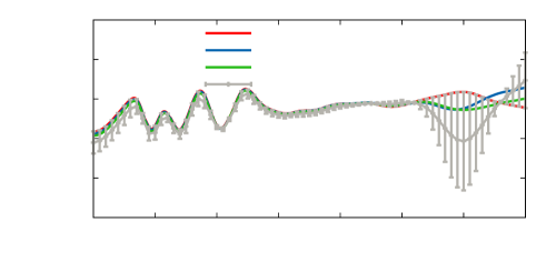
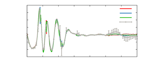
Other values of $m$ lead to qualitatively similar results, with lower masses losing convergence earlier than higher ones (this is reflected in the intervals chosen for Figure 9).

Appendix B Gauge conditions

In the numerical evolution of black holes without excision, the moving-puncture gauge, based on a second-order $\beta$-driver for the shift and the “1+log” evolution equation for the lapse [16], is the standard. The lapse prescription, however, does not work when the mean curvature $K$ can assume negative values, as the lapse would grow exponentially in these regions:

$$\partial_{t}\alpha-\beta^{i}\partial_{i}\alpha=-2K\alpha.$$ (26)

We searched for a modification of (26) that avoids the exponential runaway. In principle, one could cap the value of $\alpha$ at, say, one, resetting it to this value whenever it becomes larger. Unfortunately this modification quickly produces a sharp discontinuity in $K$, which leads to a shell of high Hamiltonian-constraint violation. This propagates then outwards, eventually affecting the entire domain.

Another potential strategy is a polynomial modification of the type:

$$\partial_{t}\alpha-\beta^{i}\partial_{i}\alpha=-2K\alpha\left(1-\left(\frac{\alpha}{\alpha_{0}}\right)^{n}\right).$$ (27)

In principle this could provide a smoother mechanism to curb the growth of $\alpha$ in the outer regions, since the modified right-hand-side has two attractive fixed points at $\alpha_{0}$ and $-\alpha_{0}$ as long as $K$ is negative (at the same time, if $n$ is large enough, the modification does not affect the behavior of the gauge near the puncture where $\alpha$ quickly becomes small). Unfortunately this gauge leads to development of a different kind of runaway behavior near the vertices of the cell, where at late times $K$ changes sign unexpectedly.

It turned out that the most successful strategy is simply to locate the maximum of $\alpha$ at each time step and normalize the lapse according to

$$\alpha\to\frac{\alpha}{\alpha_{\rm max}}.$$ (28)

This gauge leads to a well-behaved evolution, its only drawback being the computational cost of the additional reduction operation necessary to find the maximum value of the lapse at each iteration. As initial data, we set $\alpha=\psi^{-2}$ and $\beta^{i}=0$.

References

- [1] Lindquist R W and Wheeler J A 1957 Rev. Mod. Phys. 29 432–443
- [2] Wheeler J 1983 Foundations of Physics 13(1) 161–173
- [3] Clifton T and Ferreira P G 2009 Phys. Rev. D80 103503 (Preprint 0907.4109)
- [4] Clifton T, Rosquist K and Tavakol R 2012 Phys.Rev. D86 043506 (Preprint 1203.6478)
- [5] Yoo C M, Abe H, Nakao K i and Takamori Y 2012 Phys.Rev. D86 044027 (Preprint 1204.2411)
- [6] Bruneton J P and Larena J 2012 Class.Quant.Grav. 29 155001 (Preprint 1204.3433)
- [7] Bentivegna E and Korzynski M 2012 Class.Quant.Grav. 29 165007 (Preprint 1204.3568)
- [8] Bruneton J P and Larena J 2013 Class.Quant.Grav. 30 025002 (Preprint 1208.1411)
- [9] Ellis G F 2011 Classical and Quantum Gravity 28 164001 (Preprint 1103.2335)
- [10] Bentivegna E 2013 (Preprint 1305.5576)
- [11] Lichnerowicz A 1944 J. Math. Pures Appl. 23
- [12] York James W J 1971 Phys.Rev.Lett. 26 1656–1658
- [13] Loffler F, Faber J, Bentivegna E, Bode T, Diener P et al. 2012 Class.Quant.Grav. 29 115001 (Preprint 1111.3344)
- [14] Schnetter E, Hawley S H and Hawke I 2004 Class.Quant.Grav. 21 1465–1488 (Preprint gr-qc/0310042)
- [15] Yoo C M, Okawa H and Nakao K i 2013 (Preprint 1306.1389)
- [16] Alcubierre M, Bruegmann B, Diener P, Koppitz M, Pollney D et al. 2003 Phys.Rev. D67 084023 (Preprint gr-qc/0206072)