Black Hole Universe
– Time Evolution –

Abstract

Time evolution of a black hole lattice universe is simulated. The vacuum Einstein equations in a cubic box with a black hole at the origin are numerically solved with periodic boundary conditions on all pairs of faces opposite to each other. Defining effective scale factors by using the area of a surface and the length of an edge of the cubic box, we compare them with that in the Einstein-de Sitter universe. It is found that the behaviour of the effective scale factors is well approximated by that in the Einstein-de Sitter universe. In our model, if the box size is sufficiently larger than the horizon radius, local inhomogeneities do not significantly affect the global expansion law of the universe even though the inhomogeneity is extremely nonlinear.

The effect of local inhomogeneity on the global expansion of the universe has drawn much attention as one of fundamental issues in relativistic cosmology for many years. One remarkable work has been done by Lindquist and Wheeler in 1957RevModPhys.29.432 . In this work, they investigated the so-called “black hole lattice universe” composed of $N$ cells($N=$5, 8, 16, 24, 120 and 600) on the three sphere each of which has a black hole at the center. Although the lattice universe is not an exact solution, with help from an intuitive idea, it is shown that the radius of the three dimensional sphere at maximum expansion asymptotes to that of the homogeneous and isotropic dust dominated closed universe for a large value of $N$.

Recently, similar inhomogeneous universe models to the black hole lattice universe have been investigated by using analytical or numerical techniquesClifton:2009jw ; Clifton:2012qh ; Uzan:2010nw ; Bentivegna:2012ei ; Bruneton:2012cg ; Yoo:2012jz ; Bentivegna:2013xna . In this paper, we numerically construct an expanding inhomogeneous universe model which is composed of regularly aligned black holes with an identical mass $M$, and compare the cosmic expansion rate of this inhomogeneous universe model with that of the homogeneous and isotropic universe. Hereafter, we call this inhomogeneous universe model “black hole universe”.

In this paper, we use the geometrized units in which the speed of light and Newton’s gravitational constant are one, respectively. The Greek indices represent spacetime components, whereas the small Latin indices represent spatial components.

The way to construct the initial data of black hole universe is described in Ref. Yoo:2012jz . We briefly summarise it. We adopt the Cartesian coordinate system $\bm{x}=(x^{1},x^{2},x^{3})$ and focus on a cubic region $-L\leq x^{i}\leq L$ ($i=1,2,3$) with a non-rotating black hole at the origin. We call the faces of this cubic box the boundary in this paper. Because of the discrete symmetry, using conventional decomposition of the Einstein equations, we can reduce the constraint equations to three coupled Poisson equations with reflection boundary condition in the region $0\leq x^{i}\leq L$. One of the equations is the Hamiltonian constraint equation for the conformal factor and the others are momentum constraint equations for longitudinal parts of the extrinsic curvature. To solve the equations, we need to fix the functional form of the trace part of the extrinsic curvature $K$. By the volume integral of the Hamiltonian constraint equation, we get an integrability condition which implies that there must be a domain with non-vanishing $K$. Since it is the simplest and the most convenient for our purpose to select $K$ vanishing in the neighbourhood of the origin, we adopt the following functional form of $K$:

$$K(\bm{x})=-3H_{\rm eff}W(R),$$ (1)

where $H_{\rm eff}$ is a positive constant which corresponds to the effective Hubble parameter, $R:=|\bm{x}|$, and

$$W(R)=\left\{\begin{array}[]{ll}0&{\rm for}~{}0\leq R\leq\ell\\ \sigma^{-36}[(R-\sigma-\ell)^{6}-\sigma^{6}]^{6}&{\rm for}~{}\ell\leq R\leq\ell+\sigma\\ 1&{\rm for}~{}\ell+\sigma\leq R\\ \end{array}\right.,$$ (2)

with $\ell$ and $\sigma$ being constants which satisfy $\ell<\ell+\sigma<L$. An appropriate extraction of $1/R$ divergence of the conformal factor allows us to solve the coupled Poisson equations numerically. It should be noted that the value of $H_{\rm eff}$ must be determined so that the integrability condition is satisfied, that is, we cannot freely choose the parameter $H_{\rm eff}$ but must appropriately fix the value during the numerical iteration. Since the results are not significantly dependent on $\ell$ and $\sigma$, the physical dimensionless parameter which characterises the initial data is only $L/M$. In Ref. Yoo:2012jz , we could get convergence for $1.4M\leq L\leq 10M$. We adopt the case $L=2M$ as the initial data for the evolution in this paper.

The numerical time evolution is followed by COSMOS code which is an Einstein equation solver written in C++ by means of the BSSN formalism Shibata:1995we ; Baumgarte:1998te . The algorithm is based on SACRA code Yamamoto:2008js . The 4th order finite differencing in space with uni-grid and 4th order time integration with a Runge-Kutta method in Cartesian coordinates are adopted in COSMOS code. An apparent horizon solver based on Ref. Shibata:1997nc is implemented.

We write the line element of the spacetime as

$$\mathrm{d}s^{2}=-N^{2}\mathrm{d}t^{2}+\gamma_{ij}\left(\mathrm{d}x^{i}+\beta^{i}\mathrm{d}t\right)\left(\mathrm{d}x^{j}+\beta^{j}\mathrm{d}t\right).$$ (3)

In order to determine the time slicing, we adopt the following condition:

$$\left(\frac{\partial}{\partial t}-\beta^{i}\frac{\partial}{\partial x^{i}}\right)N=-2N\left(K-K_{\rm c}\right),$$ (4)

where $K_{\rm c}$ is the trace of the extrinsic curvature at the vertex $x^{i}=L~{}(i=1,2,3)$ at each time step. As for the spatial coordinates, we adopt the so-called hyperbolic gamma driver Alcubierre:2002kk with specific values of parameters given by

$$\frac{\partial\beta^{i}}{\partial t} = B^{i},$$ (5)

$$\frac{\partial B^{i}}{\partial t} = \frac{\partial\tilde{\Gamma}^{i}}{\partial t}-\frac{3}{4M}B^{i},$$ (6)

where $\tilde{\Gamma}^{i}:=-\partial_{j}\tilde{\gamma}^{ij}$ with $\tilde{\gamma}^{ij}:=\mathrm{e}^{-4\psi}\gamma^{ij}$ and $\psi:=\frac{1}{12}\ln(\det\gamma)$.

We define the cosmic expansion rate by using boundary variables on the geodesic slices Smarr-York which is occasionally called constant proper time slices. In order to know the geometry of the boundary on the geodesic slices, we need to solve timelike geodesic equations on the boundary. 3+1 decomposition of geodesic equations is clearly described in Ref. Vincent:2012kn . Using the unit vector $n_{\mu}:=-N\partial_{\mu}t$ normal to the timeslices, we can decompose the unit tangent vector field of the timelike geodesic congruence as follows:

$$u^{\mu}=E\left(n^{\mu}+V^{\mu}\right),$$ (7)

where $V^{\mu}n_{\mu}=0$. Let us represent a timelike geodesic by $x^{\mu}=x^{\mu}(t)$, where $t=x^{0}$. Then, we have Vincent:2012kn

$$\frac{\mathrm{d}E}{\mathrm{d}t} = EV^{i}\left(NK_{ij}V^{j}-\partial_{i}N\right),$$ (8)

$$\frac{\mathrm{d}V^{i}}{\mathrm{d}t} = NV^{j}\left[V^{i}\left(\partial_{j}\ln N-K_{jk}V^{k}\right)\right.$$ (10)

$$\left.+2K^{i}_{~{}j}-V^{k}\Gamma^{i}_{jk}\right]-\gamma^{ij}\partial_{j}N-V^{j}\partial_{j}\beta^{i},$$

where $\Gamma^{i}_{jk}$ is the Christoffel symbol for the spatial metric $\gamma_{ij}$, and

$$\frac{\mathrm{d}}{\mathrm{d}t} := \frac{N}{E}u^{\mu}\frac{\partial}{\partial x^{\mu}}=N\left(n^{\mu}\frac{\partial}{\partial x^{\mu}}+V^{i}\frac{\partial}{\partial x^{i}}\right)$$ (11)

$$= \frac{\partial}{\partial t}+\left(-\beta^{i}+NV^{i}\right)\frac{\partial}{\partial x^{i}}.$$ (12)

The relation between the proper time $\tau$ and the time coordinate is given by

$$\frac{\mathrm{d}\tau}{\mathrm{d}t}=1/u^{0}=\frac{N}{E}.$$ (13)

The initial conditions for geodesic equations are given by $E=1$, $V^{i}=0$ and $\tau=0$ in our simulation. It is sufficient for our purpose to consider the geodesics with $x^{3}=L$ at $\tau=0$. By the symmetry of this system, $x^{3}=L$ and $V^{3}=0$ always hold. Solving Eqs. (8), (10) and (13), we obtain the proper time in the form of $\tau=f(t,x^{A})$ ($A=1,2$). Then, the line element $\mathrm{d}l^{2}$ of the boundary $x^{3}=L$ on a hypersurface with a constant $\tau$, i.e., a geodesic slice is given by

$$\mathrm{d}l^{2} = \Biggl{[}\left(-N^{2}+\beta^{C}\beta_{C}\right)\frac{\partial_{A}f\partial_{B}f}{\left(\partial_{t}f\right)^{2}}$$ (15)

$$\hskip 42.67912pt+\gamma_{AB}-\frac{2\beta_{A}\partial_{B}f}{\partial_{t}f}\Biggr{]}\mathrm{d}x^{A}\mathrm{d}x^{B}.$$

We numerically obtain the proper area $\mathcal{A}$ of the surface $(-L\leq x^{A}\leq L,x^{3}=L)$ and the proper length $\mathcal{L}$ of the edge $(-L\leq x^{1}\leq L,x^{2}=L,x^{3}=L)$ by using this induced metric. Then, we define the effective scale factors as functions of the proper time as follows:

$$a_{\mathcal{L}}(\tau):=\mathcal{L}(\tau)~{},~{}a_{\mathcal{A}}(\tau):=\sqrt{\mathcal{A}(\tau)}.$$ (16)

Since the coarse-grained black hole universe can be regarded as a homogeneous and isotropic universe model with vanishing spatial curvature by its construction, we compare the expansion rate of the black hole universe with that in the Einstein-de Sitter(EdS) universe. To compare the effective scale factors defined by Eq. (16) with that in the EdS universe, we define a fiducial scale factor. The general form of the scale factor in the EdS universe is given by

$$a_{\rm EdS}(\tau):=a_{\rm f}\left(\tau+\tau_{\rm f}\right)^{2/3}.$$ (17)

Then we determine two parameters $a_{\rm f}$ and $\tau_{\rm f}$ by the least-square fitting of this function with the numerical data in a reliable region of $\tau$. Using this expression, the effective Hubble parameter is given by

$$H_{\rm EdS}(\tau)=\frac{2}{3}\frac{1}{\tau+\tau_{\rm f}}.$$ (18)

We performed the numerical simulation with four different resolutions:R1, R2, R3 and R4. The interval of coordinate grids for each numerical run is given by $\Delta x/M\simeq 4/59$, $4/91$, $4/123$ and $4/155$ for R1, R2, R3 and R4, respectively.

Before showing the results of effective scale factors, we note the resolution of the apparent horizon and constraint violation. At the initial moment, an almost spherical apparent horizon with the coordinate radius $R\simeq 0.5M$ exists. As shown in Fig. 1, the coordinate radius of the apparent horizon decreases as it evolves.

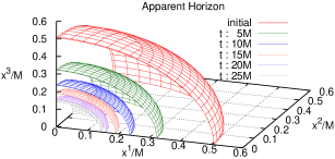
Figure 1: Apparent horizon for each time step.

At some time, our apparent horizon finder fails to find out the horizon because of the limitation of the resolution. For R4, it happens at $t\sim 25M$. While the horizon can be found, variation of the horizon area is smaller than 0.1%, which is the same order as the typical fraction of violation of the Hamiltonian constraint as is shown below. This implies that the horizon area is constant in time within our numerical precision.

As is shown in Fig. 2, after the failure in the apparent horizon search, the violation of the Hamiltonian constraint propagates outward, and the reliable region becomes narrower as time goes on. However, the numerical computation does not crash and we can proceed with the calculation.

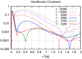
Figure 2: Evolution of the violation of the Hamiltonian constraint on the $x^{1}$-axis for R4. Zero means no violation whereas one corresponds to the largest violation.

Even after the size of apparent horizon becomes too small to be resolved, the spacetime in the vicinity of the boundary is simulated with sufficient accuracy, since the present numerical results on the behaviours of the effective scale factors pass the convergence test. In order to show the convergence clearly, we depict the root-mean-square value of errors in the Hamiltonian constraint at grid points on the boundary in Fig. 3. It is seen from this figure that the error reduces with higher spatial resolution. In the beginning of the simulation, we find accurate second order convergence that the error scales to $\Delta x^{2}$. This is because the initial data sets are given by the 2nd order Successive-Over-Relaxation method for each resolutionYoo:2012jz , although the evolution code has the 4th order accuracy.

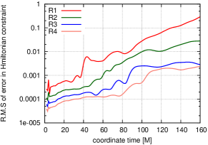
Figure 3: Root-mean-square of the errors in the Hamiltonian constraint at grid points on the boundary.

In Fig. 4, we show the effective scale factors as functions of the proper time.

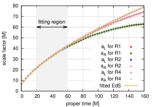
Figure 4: Effective scale factors and $a_{\rm EdS}$ as functions of $\tau$. $a_{\mathcal{A}}$ almost overlaps $a_{\mathcal{L}}$.

The fiducial scale factor $a_{\rm EdS}(\tau)$ determined by fitting with R4 is also shown. The fitting is done in the region $20M<\tau<60M$, in which the results of all runs almost coincide with each other. The given value of parameters are $a_{\rm f}\simeq 2.64M$ and $\tau_{\rm f}\simeq-3.25M$. We also show the deviation of the effective scale factors from $a_{\rm EdS}(\tau)$ in Fig. 5.

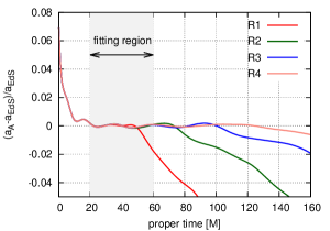
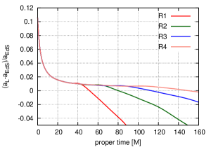
Figure 5: Deviation of the effective scale factors $a_{\rm A}$ and $a_{\rm L}$ from $a_{\rm EdS}$ for each resolution.

It can be found from Fig. 4 and 5 that the behaviour of the effective scale factors for R4 is well approximated by that of the EdS universe in the shown period of $\tau$ except for a short period in the beginning. This result is consistent with the suggestion given by the numerical simulation of the collapsing eight-black-hole latticeBentivegna:2012ei and an initial data sequenceYoo:2012jz .

It would be worth to note the reason why we have defined the effective scale factor by Eq. (16). The reason is that, since the total volume inside the box is infinite, it is hard to define the volume average in a physically meaningful manner. Therefore we do not use the spatial volume average to define the effective scale factor differently from other many related works(see e.g. Ref. Rasanen:2011ki and references therein).

The number of black holes $N_{\rm BH}$ inside the Hubble radius $H_{\rm EdS}^{-1}$ is given by

$$N_{\rm BH}\sim\frac{1}{M}\times\frac{4\pi}{3}H_{\rm EdS}^{-3}\times\frac{3}{8\pi}H_{\rm EdS}^{2}=\frac{H_{\rm EdS}^{-1}}{2M}=\frac{3}{4}\frac{\tau+\tau_{\rm f}}{M},$$ (19)

and we obtain $N_{\rm BH}\sim 100$ for $\tau\sim 130M$. As was discussed in Ref. Yoo:2012jz , it is expected that the deviation of the black hole universe from the EdS one becomes the smaller, the larger $N_{\rm BH}$ becomes, or in other words, the effects of local inhomogeneities on the global expansion law is negligible if $N_{\rm BH}$ is sufficiently large. If so, the expansion law of the black hole universe will approach to that of the EdS universe as it expands, and the present result supports this expectation.

The universe model studied here is highly idealised, since this work is the first step in the study of the universe dominated by black holes. The generalisations of our toy model to that with varieties of mass and separation etc. and the dependence of the results on them are still open issues which should be clarified in the future.

References

- (1) R. W. Lindquist and J. A. Wheeler, Rev. Mod. Phys. 29, 432 (1957).
- (2) T. Clifton and P. G. Ferreira, Phys.Rev. D80, 103503 (2009), arXiv:0907.4109.
- (3) T. Clifton, K. Rosquist, and R. Tavakol, (2012), arXiv:1203.6478.
- (4) J.-P. Uzan, G. F. Ellis, and J. Larena, Gen.Rel.Grav. 43, 191 (2011), arXiv:1005.1809.
- (5) E. Bentivegna and M. Korzynski, Class.Quant.Grav. 29, 165007 (2012), arXiv:1204.3568.
- (6) J.-P. Bruneton and J. Larena, Class.Quant.Grav. 29, 155001 (2012), arXiv:1204.3433.
- (7) C.-M. Yoo, H. Abe, K.-i. Nakao, and Y. Takamori, Phys.Rev. D86, 044027 (2012), arXiv:1204.2411.
- (8) E. Bentivegna, (2013), arXiv:1305.5576.
- (9) M. Shibata and T. Namamura, Phys.Rev. D52, 5428 (1995).
- (10) T. W. Baumgarte and S. L. Shapiro, Phys.Rev. D59, 024007 (1998).
- (11) T. Yamamoto, M. Shibata, and K. Taniguchi, Phys.Rev. D78, 064054 (2008).
- (12) M. Shibata, Phys.Rev. D55, 2002 (1997).
- (13) M. Alcubierre, B. Bruügmann, P. Diener, M. Koppiz, D. Pollney, E. Seidel, and R. Takahashi, Phys.Rev. D67, 084023 (2003).
- (14) L. Smarr and J. W. York, Jr., Phys.Rev. D17, 2529 (1978).
- (15) F. H. Vincent, E. Gourgoulhon, and J. Novak, Class.Quant.Grav. 29, 245005 (2012), arXiv:1208.3927.
- (16) S. Rasanen, Class. Quant. Grav. 28, 164008 (2011) [arXiv:1102.0408 [astro-ph.CO]].