Slipping motion of large neutrally-buoyant particles in turbulence

Abstract

Direct numerical simulations are used to investigate the individual dynamics of large spherical particles suspended in a developed homogeneous turbulent flow. A definition of the direction of the particle motion relative to the surrounding flow is introduced and used to construct the mean fluid velocity profile around the particle. This leads to an estimate of the particle slipping velocity and its associated Reynolds number. The flow modifications due to the particle are then studied. The particle is responsible for a shadowing effect that occurs in the wake up to distances of the order of its diameter: the particle pacifies turbulent fluctuations and reduces the energy dissipation rate compared to its average value in the bulk. Dimensional arguments are presented to draw an analogy between particle effects on turbulence and wall flows. Evidence is obtained on the presence of a logarithmic sublayer at distances between the thickness of the viscous boundary layer and the particle diameter $D_{\mathrm{p}}$. Finally, asymptotic arguments are used to relate the viscous sublayer quantities to the particle size and the properties of the outer turbulence. It is shown in particular that the skin-friction Reynolds number behaves as $Re_{\tau}\propto(D_{\mathrm{p}}/\eta)^{4/3}$.

1 Introduction

Several natural and industrial phenomena require to model the transport of finite-size and mass particles suspended in a turbulent incompressible flow. This is for instance the case for air pollutants, plankton in the ocean, and industrial mixtures. When the particle size is much smaller than the smallest active scale of the flow (the Kolmogorov dissipative scale $\eta$ in turbulence) and when their Reynolds number defined with their relative velocity to the fluid is sufficiently small, the surrounding flow can be described by the linear Stokes equation (see Gatignol, 1983; Maxey & Riley, 1983). This approach leads to model small particles in terms of point-particles for which an equation of motion can be explicitly written. It has then been shown that inertia is responsible for particle clustering, a phenomenon usually referred to as preferential concentration, and for non-trivial dynamical and statistical properties that can be characterized in terms of the particle Stokes number and of the flow properties (see, e.g., Toschi & Bodenschatz, 2009). However much less is known for particles with sizes comparable or larger than $\eta$, which can typically have Reynolds numbers larger than unity. Their dynamics can hardly be modeled because writing an explicit equation of motion requires fully solving the non-linear Navier–Stokes equation in the vicinity of the particle. To tackle this problem, one has to make use either of advanced experimental particle-tracking techniques or of demanding direct numerical simulations.

Many recent experimental developments aimed at characterizing the dynamical properties of finite-size, neutrally buoyant particles (with the same mass density as the fluid). Detailed measurements by Qureshi et al. (2007), Xu & Bodenschatz (2008), Volk et al. (2011) and Zimmermann et al. (2011) of the translation and angular accelerations suggested that, to a large extent, finite-size effects can be related to known turbulent properties calculated at a length scale given by the particle size. Such approaches are thus implicitly assuming that the presence of the particle is not altering the fine scaling properties of the velocity and pressure fields in its vicinity. While in direct numerical simulations both the particle motion and the surrounding fluid flow are by essence always known, such simultaneous measurements require in experiments an astute setup, as those described by Khalitov & Longmire (2002), by Bellani et al. (2012) or by Klein et al. (2012). In any case, tracking experimentally or numerically a particle together with the surrounding flow requires a heavy machinery that complicates the obtention of acute statistics. It can be for instance particularly laborious to determine joint distributions of the fluid velocity and the particle acceleration for an isolated particle in a high-Reynolds turbulent flow. Primarily for that reason, most of the numerical studies have focused either on a fixed particle in a developed turbulent flow or on the modulation of turbulence by many particles (see, e.g., Balachandar & Eaton, 2010, for a review).

In this paper we make use of a pseudo-spectral solver for the Navier–Stokes equation, associated to an immersed boundary method to impose no-slip boundary conditions, in order to study neutrally buoyant spherical particles which are suspended in a developed turbulent flow and whose diameters $D_{\mathrm{p}}$ are within the inertial range. Our focus is mainly on the local modifications of the flow in the neighborhood of the particle. A first objective is to understand the instantaneous direction of the particle slip with respect to the fluid. We propose a definition that is based on the averaged direction of the fluid flux in several shells surrounding the spherical particle. This allows us to compute a mean flow around the moving particle and to estimate an effective particle Reynolds number. We then investigate the local modifications of the surrounding turbulent flow due to the presence of the particle. We show that, while kinetic energy dissipation is enhanced in the boundary layer, the particle is calming down turbulent fluctuations in its wake up to distances of the order of its diameter $D_{\mathrm{p}}$. Scaling arguments are used to understand the growth of the turbulent fluctuations as a function of the distance to the particle. Similarly to usual wall flows, they show the presence of a logarithmic law involving a friction velocity and a wall distance that can be used to collapse the data associated to different particle sizes. Such arguments, once put together with Kolmogorov scaling for the outer turbulence, can also be used to show that the particle friction Reynolds number scales as $\mbox{{Re}}_{\tau}\propto(D_{\mathrm{p}}/\eta)^{4/3}$.

The paper is organized as follows. In §2, after a short description of our settings and of the numerical method, we introduce a definition of the instantaneous direction of the particle slip to obtain the mean flow around it. The effects of the particle on the surrounding turbulent fluctuations are then discussed in §3. Finally, concluding remarks are encompassed in §4.

2 The slip velocity

$N^{3}$	$\delta x$	$\nu$	$u_{\mathrm{rms}}$	$\varepsilon$	$\eta$	$\tau_{\eta}$	$L$	$T_{L}$	$\mbox{{Re}}_{\lambda}$
$1024^{3}$	$6.13\cdot 10^{-3}$	$1.8\cdot 10^{-4}$	$0.19$	$4.5\cdot 10^{-3}$	$6.0\cdot 10^{-3}$	0.20	1.6	8.2	$160$

Table 1: Parameters of the numerical simulations. $N^{3}$: number of collocation points, $\delta x$: grid spacing, $\nu$: kinematic viscosity, $u_{\mathrm{rms}}$: root-mean-square velocity, $\varepsilon$: mean kinetic energy dissipation rate, $\eta=(\nu^{3}/\varepsilon)^{1/4}$: Kolmogorov dissipation length scale, $\tau_{\eta}=(\nu/\varepsilon)^{1/2}$: Kolmogorov time scale, $L=u_{\mathrm{rms}}^{3}/\varepsilon$: integral scale, $T_{L}=L/u_{\mathrm{rms}}$: large-eddy turnover time, $\mbox{{Re}}_{\lambda}=\sqrt{15\,u_{\mathrm{rms}}L/\nu}$: Taylor-microscale Reynolds number.

To address numerically the problem of large-particle dynamics in a turbulent flow, we make use of a standard pseudo-Fourier-spectral solver of the Navier–Stokes equations in which the no-slip boundary condition at the particle surface is imposed by an immersed boundary technique. The neutrally buoyant particle translational and rotational dynamics is integrated using Newton’s equations. Details and benchmarks of the method for fixed particles can be found in Homann et al. (2013). A similar method has been used in Homann & Bec (2010) to investigate the dynamics of particles with sizes of the order of the Kolmogorov scale $\eta$. We report here results on larger particles. Three independent simulations are performed with three different particle diameters $D_{\mathrm{p}}\simeq 17$, $34$, and $67\eta$. In each case, a large-scale forcing is maintaining the transporting turbulent flow in a statistical steady state with a Taylor-microscale Reynold number $\mbox{{Re}}_{\lambda}\approx 160$. The parameters of the simulations are listed in Tab. 1. Three different runs have been performed, each with a single particle of size $D_{p}=0.1=17\,\eta=L/16$, $D_{p}=0.2=34\,\eta=L/8$, and $D_{p}=0.4=67\,\eta=L/4$, respectively. The turbulent quantities reported in Tab. 1 vary by less than 2% between the different runs.

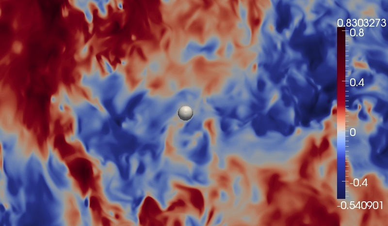
(a) $\vec{u}\cdot\vec{e}_{x}$

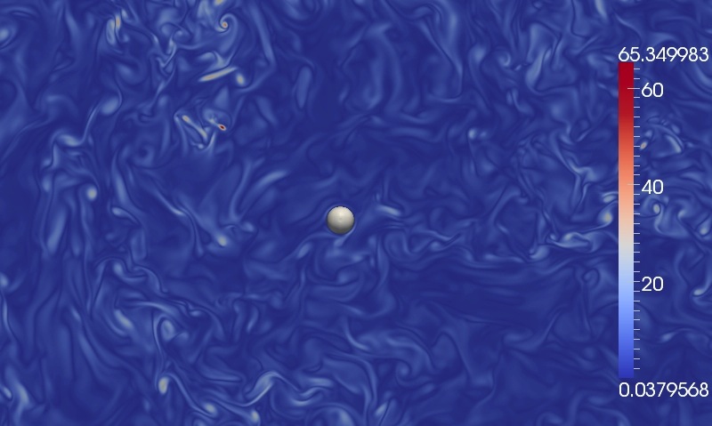
(b) $|\vec{\omega}|$

Figure 1: (Colour online) Snapshot of one component of the velocity (a) and of the vorticity modulus (b) in a thin slice of the flow around the particle.

Figure 1 shows snapshots (at the same time) of a component of the fluid velocity (a) and of the modulus of the vorticity (b) in a plane passing through the center of the particle for $D_{\mathrm{p}}=34\eta$. One clearly sees that in both cases, being focusing on either large or small-scale fluctuations, the fluid flow around the particle varies on scales of the order of its size. This points out one of the key questions in understanding the dynamics of finite-size particles, that is to define the fluid velocity at the particle position. This quantity is of particular importance to evaluate the relative motion (the slip) of the particle with respect to the carrier flow. All models for particle dynamics consist in expressing the drag and lift forces exerted by the flow in terms of this slip velocity.

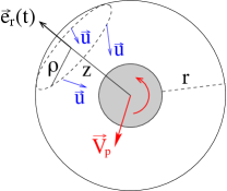
Figure 2: (Colour online) Sketch of the definition of the direction of slip $\vec{e}_{r}$ on a shell of radius $r$ and of the associated instantaneous coordinates $z$ and $\rho$.

We aim here at defining an instantaneous direction of the motion of the particle relative to the fluid. The idea we propose is to evaluate this direction on different shells surrounding the particle and at each instant of time. For that we have stored with a sufficiently high frequency the velocity field in several concentric spheres centered on the particle. On the shell $\mathcal{S}_{r}$, which is at a distance $r$ from the particle surface, we define the direction of motion $\vec{e}_{r}$ as

$$\vec{e}_{r}(t)=\vec{\Phi}_{r}(t)/|\vec{\Phi}_{r}(t)|,\quad\mbox{where }\vec{\Phi}_{r}(t)=\int_{\mathcal{S}_{r}}\left(\vec{u}(\vec{x},t)-\vec{V}_{\mathrm{p}}(t)\right)\cdot\vec{n}\,\,\mathrm{d}\vec{S},$$ (1)

where $\vec{u}$ and $\vec{V}_{\mathrm{p}}$ are the fluid and the particle translational velocity, respectively, $\vec{n}$ is the vector normal to the shell (see Fig. 2). In other words, we perform on each shell an average of the direction weighted by the fluid mass flux, so that $\vec{e}_{r}$ points in the direction of the flux on the shell at distance $r$. This choice is physically motivated as the fluid enters such a shell upstream and exits in the wake. If the particle was moving in a laminar flow, the direction $\vec{e}_{r}$ would be, by symmetry, independent of $r$ and exactly aligned with this motion. When the particle creates a wake in an unsteady flow, the direction $\vec{e}_{r}(t)$ depends on both time and $r$. Once the direction $\vec{e}_{r}$ is defined, one can project on it the velocity difference $\vec{u}-\vec{V}_{\mathrm{p}}$ and perform a time average to construct the mean velocity profile of the flow relative to the particle

$$U_{\mathrm{rel}}(\rho,z)=\left\langle\left(\vec{u}(\vec{x},t)-\vec{V}_{\mathrm{p}}(t)\right)\cdot\vec{e}_{r}\right\rangle,$$ (2)

with $z=(\vec{x}-\vec{X}_{\mathrm{p}}(t))\cdot\vec{e}_{r}$ and $\rho=[\|\vec{x}-\vec{X}_{\mathrm{p}}(t)\|^{2}-z^{2}]^{1/2}$. The angular brackets $\langle\cdot\rangle$ designate here the temporal average. The coordinates $z$ and $\rho$, which are defined at each instant of time, are in the direction of $\vec{e}_{r}$ and perpendicular to it, respectively. By rotational symmetry around the axis defined by $\vec{e}_{r}$, the mean profile $U_{\mathrm{rel}}$ depends on $z$ and $\rho$ only and not on the angle.

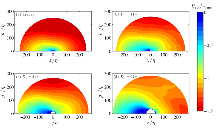
Figure 3: (Colour online) Temporal- and angle-averaged relative velocity (definition with flux) of the fluid projected on the direction of motion for (a) a tracer and (b) $D_{\mathrm{p}}=17\eta$, (c) $D_{\mathrm{p}}=34\eta$, and (d) $D_{\mathrm{p}}=67\eta$.

Figure 3 represents the measured average velocity profile for a tracer and for the three particle sizes. The relative motion of the fluid with respect to the particle is from $z>0$ to $z<0$. In all four cases, the upstream and downstream velocities are clearly asymmetric. Also, when the particle radius increases, one observes the development in the wake of a region where the flow is calmed down. However a large part of the information contained in the mean relative velocity $U_{\mathrm{rel}}$ is purely due to kinematics. This is clear when interested in the case of the tracer: the surrounding flow is trivially not affected by its presence but the conditioning in terms of the instantaneous flux direction $\vec{e}_{r}$ prevents the average relative velocity profile from vanishing and singles out the growth of turbulent velocity increments $\sim r^{1/3}$. The observed asymmetry relates to the fact that the negative longitudinal velocity differences (on the right) are more likely to be larger than the positive ones (on the left); this can be interpreted as a consequence of the 4/5 law and of the resulting skewness of velocity differences in turbulence.

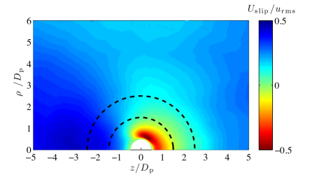
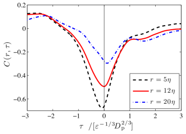
Figure 4: (Colour online) (a) slip velocity $U_{\mathrm{slip}}$ for $D_{\mathrm{p}}=34\eta$ defined as the difference between the mean relative velocity profile $U_{\mathrm{rel}}$ around the particle and that around a tracer; the two black dashed circles represent distance equal to $D_{\mathrm{p}}$ and $2D_{\mathrm{p}}$ from the particle surface. (b) Time correlation $C(r,\tau)=\langle\vec{F}(t+\tau)\cdot\vec{e}_{r}(t)\rangle/\langle|\vec{F}|^{2}\rangle^{1/2}$ between the force at time $t+\tau$ and the direction of motion at time $t$ for three values of the shell distance $r$ and for $D_{\mathrm{p}}=34\eta$.

Actually, the details of the particle slip and of the flow modifications due to its presence can be obtained by comparing the average profiles with a particle to that without it. One observes in Fig. 3 that the most noticeable differences occur on scales of the order of the particle diameter. This is even clearer in Fig. 4(a), which represents for $D_{\mathrm{p}}=34\eta$ the “slip velocity” profile defined as

$$U_{\mathrm{slip}}(\rho,z)=U_{\mathrm{rel}}(\rho,z)-U_{\mathrm{rel}}^{\mathrm{tracer}}(\rho,z).$$ (3)

This quantity is the difference between two velocity differences. The four terms it contains can in principle be grouped in two contributions: the difference between the fluid velocity with and without the particle, which accounts for the flow modifications due to its presence, and minus the difference between the particle velocity and the velocity of a tracer that would be at the particle location. The first term comprises all the space dependency. One observes from Fig. 4(a) that the flow modifications due to the particle are up to distances of the order of its diameter and vanish far from the particle. At sufficiently large distances, $U_{\mathrm{slip}}$ attains a positive constant coming from the second contribution. This limit, that we denote $U_{\mathrm{slip}}^{\infty}$ can be used to define a difference between the particle velocity and that of the fluid at the particle location, that is a typical slip velocity. We can make use of $U_{\mathrm{slip}}^{\infty}$ in order to define a particle Reynolds number $Re_{p}=U_{\mathrm{slip}}^{\infty}\,D_{\mathrm{p}}/\nu$. We obtain:
  - for $D_{\mathrm{p}}=17\eta$: $U_{\mathrm{slip}}^{\infty}\approx 0.049$ and $Re_{p}\approx 27$, - for $D_{\mathrm{p}}=34\eta$: $U_{\mathrm{slip}}^{\infty}\approx 0.052$ and $Re_{p}\approx 58$, - for $D_{\mathrm{p}}=67\eta$: $U_{\mathrm{slip}}^{\infty}\approx 0.057$ and $Re_{p}\approx 126$.
The typical turbulent fluid velocity fluctuation $\propto(\varepsilon D_{\mathrm{p}})^{1/3}$ at a separation $D_{\mathrm{p}}$ is from 1.5 to 2 times larger than these values of the slip velocity. Note that the definition of a slip velocity that we are using here is based on the instantaneous direction of motion $\vec{e}_{r}$ introduced earlier. It thus differs from the slip definitions based on statistical arguments, such as that used by Bellani & Variano (2012).

One step further to assess the validity of the proposed definition of the relative motion direction $\vec{e}_{r}$ consists in looking at its alignement with the force $\vec{F}$ exerted by the fluid onto the particle. For that we define the correlation $C(r,\tau)=\langle\vec{F}(t+\tau)\cdot\vec{e}_{r}(t)\rangle/\langle|\vec{F}|^{2}\rangle^{1/2}$ between the force at time $t+\tau$ and the direction of motion of the shell at distance $r$ and at time $t$. As seen from Fig. 4(b) the two vectors are anti-correlated. The anti-correlation is maximal very close to the particle surface where the flow is trivially enslaved to the solid motion because of the no-slip boundary condition. However, the optimal lag $\tau$ which maximizes the anti-correlation is there negative. This means that the force is there imposing the direction $\vec{e}_{r}$ of the local motion. The anti-correlation decreases when $r$ increases and becomes very small when $r\gg D_{\mathrm{p}}$. At sufficiently large distances, the minimum of correlation is attained for a positive value of the time lag $\tau$. It means that sufficiently far from the particle, the flow direction is in advance on that of the force. There is thus a specific value of $r$, of the order of $D_{\mathrm{p}}/2$, for which the optimal lag vanishes and the direction of the force is almost synchronized with that of the relative motion. This indicates that the fluid-particle interactions occur at distances up to the order of the particle diameter $D_{\mathrm{p}}$, as already observed by Naso & Prosperetti (2010). Also, we find that a part of the force exerted by the fluid corresponds to a drag in the direction $\vec{e}_{r}$ of the relative motion.

3 Turbulence statistics in the vicinity of the particle

3.1 Imprint on the kinetic energy and the dissipation rate

We now turn to the influence of the particle on higher-order statistics of the fluid velocity field. Figure 5(a) shows the “particle-anchored” second-order longitudinal structure function defined as

$$S^{\parallel}_{2}(r)=\left\langle\left[\left(\vec{u}(\vec{x},t)-\vec{V}_{\mathrm{p}}(t)\right)\cdot\vec{n}\right]^{2}\right\rangle,$$ (4)

where $\vec{n}$ is the unit vector in the direction of $\vec{x}-\vec{X}_{\mathrm{p}}$ and $r=\|\vec{x}-\vec{X}_{\mathrm{p}}\|-D_{\mathrm{p}}/2$ is the distance from $\vec{x}$ to the particle surface. Using the instantaneous and $r$-dependent definition of the relative motion direction $\vec{e}_{r}(t)$ of previous section, the average can be decomposed in an upstream contribution (for $\vec{x}$ in a cone of 90^o in the direction of $\vec{e}_{r}$), a downstream contribution (in a cone of 90^o in the direction of $-\vec{e}_{r}$) and a transverse contribution (remaining values). One observes in Fig. 5(a) that the velocity fluctuations are apparently enhanced upstream the particle. This is essentially due to the average flow modifications as the flow is accelerated when approaching the particle and encounters steep gradients. In principle one would expect a similar behaviour downstream as the flow is there decelerated. However we observe the reverse phenomenon as the large-$r$ asymptotics is reached from below. This indicates that the particle is calming down turbulence in its wake.

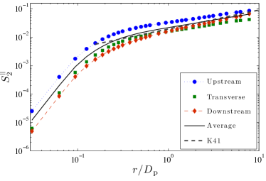
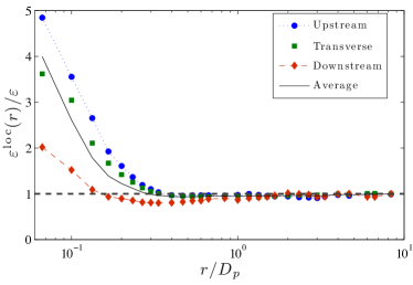
Figure 5: (Colour online) (a) Particle-anchored second order structure function (the K41 line stands for $S_{2}^{\parallel}=C_{2}(\varepsilon r)^{2/3}$ with $C_{2}=2.1$) and (b) local dissipation rate in different regions around the particle as a function of the distance to its surface for $D_{p}=34\eta$.

This effect is even more visible in the profile of the average kinetic energy dissipation rate $\varepsilon^{\mathrm{loc}}(r)$ computed as a function of the distance $r$ to the particle surface and conditioned on the upstream, downstream and transversal sectors. As seen from Fig. 5(b), while energy dissipation is strongly enhanced in all directions in the vicinity of the particle, its downstream value is below $90\%$ of its average up to distances of the order of the particle diameter. This indicates again that turbulence is more quiet downstream.

The particle is thus creating a shadow in its wake. An explanation relies on the fact that all turbulent structures of sizes of the order of $D_{\mathrm{p}}$ are not anymore present in the downstream flow. In addition, given the pretty low values of the Reynolds numbers estimated in previous section, the particle wake is not strong enough to inject a significant amount of turbulent kinetic energy. This shadowing effect seems to depend only weakly on the particle size, up to the short range of values we have investigated and the accuracy of our simulations.

3.2 Analogy with wall turbulence

To analyse more precisely the particle size dependence of the disturbed flow, we make use of an approach similar to that used in wall turbulence. A first important difference is that in the case of particles the “bulk flow” is not a input data, so that our approach relies on what is happening in the immediate neighborhood of the boundary. A second difference is that, because of the isotropy of the particle dynamics, the velocity field averages to zero and there is no notion of mean velocity profile. For this reason, we make use of the root-mean-square velocity difference between the flow and the particle surface in the tangential directions

$$U(r)=\left\langle\frac{1}{2}\left\|\vec{u}-(\vec{u}\cdot\vec{n})\,\vec{n}-\vec{V}_{\mathrm{p}}-\frac{D_{\mathrm{p}}}{2}\,\vec{\Omega}_{\mathrm{p}}\times\vec{n}\right\|^{2}\right\rangle^{1/2},$$ (5)

where $\vec{n}$ is the unit vector normal to the spherical particle and $\vec{\Omega}_{\mathrm{p}}$ is the particle angular velocity. $U^{2}(r)$ is nothing but the second-order “particle-anchored” transverse structure function. Our numerical data allows us to measure a wall shear stress as

$$\tau_{\mathrm{w}}=\nu\left.\left[\frac{\mathrm{d}U}{\mathrm{d}r}\right]\right|_{r=0},$$ (6)

As in the case of wall flows (see, e.g., Pope, 2000), this quantity, together with the viscosity $\nu$, defines all relevant quantities of the viscous boundary layer surrounding the particle, namely the friction velocity $u_{\tau}=\sqrt{\tau_{\mathrm{w}}}$, the viscous lengthscale $\delta_{\nu}=\nu/u_{\tau}$, and the friction Reynolds number $Re_{\tau}=u_{\tau}\,D_{\mathrm{p}}/\nu$. Also, $U$ and $r$ can be written in wall units by introducing $U^{+}=U/u_{\tau}$ and $r^{+}=r/\delta_{\nu}$.

The fluid velocity at a distance $r$ from a particle is completely determined by $u_{\tau}$, $\delta_{\nu}$, $D_{\mathrm{p}}$, $L$, and $\mbox{{Re}}_{\lambda}$. Dimensional analysis then suggests to write

$$\frac{\mathrm{d}U}{\mathrm{d}r}=\frac{u_{\tau}}{r}\,\Psi({r}/{{\delta}_{\nu}},\,{r}/{{D}_{p}},\,{r}/{L},\mbox{{Re}}_{\lambda}),$$ (7)

where we have non-dimensionalized lenghtscales with $r$ and velocities with $u_{\tau}$. We next make use of the scale separation $\delta_{\nu}\ll D_{\mathrm{p}}\ll L$ to evidence different layers.

• $r\ll\delta_{\nu}$ corresponds to the viscous sublayer where by construction $U^{+}\simeq r^{+}$.

• $\delta_{\nu}\ll r\ll D_{\mathrm{p}}$ is the outer layer. We have $\mathrm{d}U/\mathrm{d}r\simeq(u_{\tau}/r)\,\Psi_{\star}(\mbox{{Re}}_{\lambda})$, where $\Psi_{\star}(\mbox{{Re}}_{\lambda})=\Psi(\infty,0,0,\mbox{{Re}}_{\lambda})$. As in wall turbulence, this leads to the log-law

  $$U^{+}=C+\Psi_{\star}(\mbox{{Re}}_{\lambda})\,\ln r^{+}.$$ (8)

• $D_{\mathrm{p}}\ll r\ll L$ corresponds to distances far from the particle where turbulent fluid statistics are recovered. In the limit of very large Reynolds numbers we can assume that $r/L\to 0$. At large distances from the particle, the behaviour of $U$ should be given by the fluid velocity second-order structure function. According to Kolmogorov 1941 scaling, we expect $U^{2}\simeq(4/3)\,C_{2}\,(\varepsilon r)^{2/3}$. This implies that for $r/D_{\mathrm{p}}\to\infty$, the dimensionless function $\Psi$ has to diverge as a power law (with exponent $\alpha$ and a constant $\Psi_{\infty}$ that depends on the outer Reynolds number), so that $\mathrm{d}U/\mathrm{d}r\simeq\Psi_{\infty}(\mbox{{Re}}_{\lambda})\,(u_{\tau}/r)\,(r/D_{\mathrm{p}})^{\alpha}$. when $r\gg D_{\mathrm{p}}$. We hence find that $\alpha=1/3$ and $u_{\tau}\propto(\varepsilon D_{\mathrm{p}})^{1/3}$.

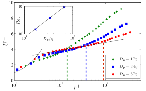
Figure 6: (Colour online) Average transverse velocity amplitude $U$ as a function of the distance to the particle surface in wall units for three different particle sizes; the black solid curve on the left refers to the viscous sublayer; the black solid line is a fit to the logarithmic law of the form $U^{+}=2.8+0.45\ln r^{+}$; the three dashed vertical lines represents the values of $D_{\mathrm{p}}$ in wall units. Inset: Friction Reynolds number $Re_{\tau}$ as a function of the particle diameter (crosses); the black line corresponds to $Re_{\tau}=0.35\,(D_{\mathrm{p}}/\eta)^{4/3}$.

These three asymptotics can be observed in Fig. 6 where the amplitude $U$ of the tangential velocity difference is represented as a function of the distance to the particle surface. One clearly sees a log-law region that becomes wider when $D_{\mathrm{p}}$ increases. The relationship $u_{\tau}\propto(\varepsilon D_{\mathrm{p}})^{1/3}$ that was obtain by matching the large-$r$ asymptotics to the behaviour of turbulent structure functions implies that the viscous lengthscale obeys $\delta_{\nu}/\eta\propto(D_{\mathrm{p}}/\eta)^{-1/3}$ and that the friction Reynolds number depends on the particle size as $Re_{\tau}\propto(D_{p}/\eta)^{4/3}$. This latter behaviour is confirmed numerically as seen from the inset of Fig. 6. Note that these values differ roughly by a factor 2 from those obtained in §2 from our estimate of the slip velocity. To conclude this analysis, let us stress that the simple dimensional arguments developed here and which seem to be numerically confirmed, show that the important parameter to specify the fluid flow in the particle neighborhood is the non-dimensional ratio $D_{\mathrm{p}}/\eta$.

4 Concluding remarks

In this paper, we have investigated the interactions between a large particle and the turbulent flow surrounding it. We proposed a definition of an instantaneous direction in which the particle slips with respect to the fluid using the mass fluxes in different concentric shells centered on the particle. This definition allowed us to construct a mean flow around the particle and to define a typical slip velocity. We next turned to the effect of the particle on the properties of the surrounding turbulence. We have seen that kinetic energy dissipation is reduced in the wake, so that particles are responsible for a kind of shadowing effect on the flow. Finally, we have presented dimensional arguments analogous to those used for wall turbulence in order to characterize the velocity fluctuations in the direction transverse to the particle surface. We have shown the presence of a log law and related the viscous sublayer properties to the particle size and the carrier flow turbulence.

A potential application of our work relates to the design of models for the dynamics of large-size particles suspended in a turbulent flow. In most practical situations that are encountered in engineering or atmospheric sciences, the flow is under-resolved (as for instance in large-eddy simulations) and the dynamics of particles with large inertial-range sizes still below the cutoff scale is approached by point particles (see, e.g., Balachandar, 2009, for more details). The force acting on the particle is then approximated by the standard drag model, possibly including empirical corrections due to the presence of turbulence in the particle surrounding. The approach we have proposed here opens new ways in tackling such issues in terms of slip direction, shell averages, and log layer. This goes beyond the scope of the present work as it will require a huge computational investment to study, for instance, the correlations between the force and the surrounding flow.

Finally, it is important to mention that we have focused here on isolated large-size particles. Our results do not straightforwardly extend to the interactions between several of them. However, in very dilute settings, we expect the modulation of turbulence by a dispersed phase to be affected by our findings. As seen in §3.1, the change in energy dissipation is two-fold: on the one hand, it is increased in the immediate vicinity of the particle and, on the other hand, it is weakened in its wake. This non-uniform effect can have non-trivial consequences on the coupling between the flow and the particles, to which possible collective effects can add up. One can for instance imagine that particles gather even if they are neutrally buoyant and unaffected by preferential concentration, the main mechanism being a collective shadowing of turbulent fluctuations that prevent eddies from separating them.

We thank M. Gibert for useful discussions. This work was performed using HPC resources from GENCI-IDRIS (Grant 026174) and from FZ Jülich (project HBO22). Support from COST Action MP0806 is kindly acknowledged. The research leading to these results has received funding from the European Research Council under the European Community’s Seventh Framework Program (FP7/2007-2013, Grant Agreement no. 240579).

References

- Balachandar (2009) Balachandar, S. 2009 A scaling analysis for point–particle approaches to turbulent multiphase flows. Int. J. Multiphase Flow 35, 801 – 810.
- Balachandar & Eaton (2010) Balachandar, S & Eaton, J.K. 2010 Turbulent dispersed multiphase flow. Ann. Rev. Fluid Mech. 42, 111–133.
- Bellani et al. (2012) Bellani, G., Byron, M.L., Collignon, A.G., Meyer, C.R. & Variano, E.A. 2012 Shape effects on turbulent modulation by large nearly neutrally buoyant particles. J. Fluid Mech. 712, 41–60.
- Bellani & Variano (2012) Bellani, G & Variano, E A 2012 Slip velocity of large neutrally buoyant particles in turbulent flows. New J. Phys. 14 (12), 125009.
- Gatignol (1983) Gatignol, R. 1983 The Faxén formulae for a rigid sphere in an unsteady non-uniform Stokes flow. J. Méc. Théor. Appl. 1, 143–160.
- Homann & Bec (2010) Homann, H. & Bec, J. 2010 Finite-size effects in the dynamics of neutrally buoyant particles in turbulent flow. J. Fluid Mech. 651, 81.
- Homann et al. (2013) Homann, H., Bec, J. & Grauer, R. 2013 Effect of turbulent fluctuations on the drag and lift forces on a towed sphere and its boundary layer. J. Fluid Mech. 721, 155–179.
- Khalitov & Longmire (2002) Khalitov, D. A. & Longmire, E. K. 2002 Simultaneous two-phase piv by two-parameter phase discrimination. Experiments in Fluids 32, 252–268.
- Klein et al. (2012) Klein, S., Gibert, M., Bérut, A. & Bodenschatz, E. 2012 Simultaneous 3d measurement of the translation and rotation of finite size particles and the flow field in a fully developed turbulent water flow. Meas. Sci. Technol. 24, 024006.
- Maxey & Riley (1983) Maxey, M.R. & Riley, J.J. 1983 Equation of motion for a small rigid sphere in a nonuniform flow. Phys. Fluids 26, 883–889.
- Naso & Prosperetti (2010) Naso, A. & Prosperetti, A. 2010 The interaction between a solid particle and a turbulent flow. New J. Phys. 12, 033040.
- Pope (2000) Pope, S.B. 2000 Turbulent flows. Cambridge: Cambridge University Press.
- Qureshi et al. (2007) Qureshi, N., Bourgoin, M., Baudet, C., Cartellier, A. & Gagne, Y. 2007 Turbulent transport of material particles: An experimental study of finite size effects. Phys. Rev. Lett. 99, 184502.
- Toschi & Bodenschatz (2009) Toschi, F. & Bodenschatz, E. 2009 Lagrangian properties of particles in turbulence. Ann. Rev. Fluid Mech. 41, 375–404.
- Volk et al. (2011) Volk, R., Calzavarini, E., Lévêque, E. & Pinton, J.-F. 2011 Dynamics of inertial particles in a turbulent von kármán flow. J. Fluid Mech. 668, 223–235.
- Xu & Bodenschatz (2008) Xu, H. & Bodenschatz, E. 2008 Motion of inertial particles with sizes larger than Kolmogorov scales in turbulent flows. Physica D 237, 2095–2100.
- Zimmermann et al. (2011) Zimmermann, R., Gasteuil, Y., Bourgoin, M., Volk, R., Pumir, A. & Pinton, J.-F. 2011 Rotational intermittency and turbulence induced lift experienced by large particles in a turbulent flow. Phys. Rev. Lett. 106, 154501.