$UV$-Continuum Slopes of $>$4000 $z\sim 4$-8 Galaxies from the HUDF/XDF, HUDF09, ERS, CANDELS-South, and CANDELS-North Fields

Abstract

We measure the UV-continuum slope $\beta$ for over 4000 high-redshift galaxies over a wide range of redshifts $z\sim 4$-8 and luminosities from the HST HUDF/XDF, HUDF09-1, HUDF09-2, ERS, CANDELS-N, and CANDELS-S data sets. Our new $\beta$ results reach very faint levels at $z\sim 4$ ($-$15.5 mag: $0.006L_{z=3}^{*}$), $z\sim 5$ ($-$16.5 mag: $0.014L_{z=3}^{*}$), and $z\sim 6$ and $z\sim 7$ ($-$17 mag: $0.025L_{z=3}^{*}$). Inconsistencies between previous studies led us to conduct a comprehensive review of systematic errors and develop a new technique for measuring $\beta$ that is robust against biases that arise from the impact of noise. We demonstrate, by object-by-object comparisons, that all previous studies, including our own and those done on the latest HUDF12 dataset, suffered from small systematic errors in $\beta$. We find that after correcting for the systematic errors (typically $\Delta\beta\sim 0.1$-0.2) all $\beta$ results at $z\sim 7$ from different groups are in excellent agreement. The mean $\beta$ we measure for faint ($-$18 mag: $0.1L_{z=3}^{*}$) $z\sim 4$, $z\sim 5$, $z\sim 6$, and $z\sim 7$ galaxies is $-$2.03$\pm$0.03$\pm$0.06 (random and systematic errors), $-$2.14$\pm$0.06$\pm$0.06, $-$2.24$\pm$0.11$\pm$0.08, and $-$2.30$\pm$0.18$\pm$0.13, respectively. Our new $\beta$ values are redder than we have reported in the past, but bluer than other recent results. Our previously reported trend of bluer $\beta$’s at lower luminosities is confirmed, as is the evolution to bluer $\beta$’s at high redshifts. $\beta$ appears to show only a mild luminosity dependence faintward of $M_{UV,AB}\sim-19$ mag, suggesting that the mean $\beta$ asymptotes to $\sim-$2.2 to $-$2.4 for faint $z\geq 4$ galaxies. At $z\sim 7$, the observed $\beta$’s suggest non-zero, but low dust extinction, and they agree well with values predicted in cosmological hydrodynamical simulations.

1. Introduction

An important frontier in the study of very high redshift galaxies remains the study of their stellar populations. Galaxies within a few hundred million years of the Big Bang are expected to be quite different from galaxies at lower redshift, with significantly younger ages and lower metallicities. For very young and chemically immature systems, changes in the stellar population could include a transition to a more top-heavy IMF (e.g., Bromm & Larson 2004), evolution in the dust composition (e.g., due to changes in the dust production mechanism: Maiolino et al. 2004), as well as a much lower dust extinction overall (e.g., Bouwens et al. 2009; Finlator et al. 2011; Dayal & Ferrara 2012).

Over the last few years, considerable progress has been made in characterizing the changes in stellar populations of galaxies back to the earliest times. We have constraints on both the ages and emission line strengths of galaxies at $z\gtrsim 4$ (e.g., Stark et al. 2009; Labbé et al. 2010; González et al. 2011; González et al. 2012; Stark et al. 2013; Labbé et al. 2013; Lee et al. 2012; Oesch et al. 2013a), and we have measurements of the $UV$-continuum slopes $\beta$ ($f_{\lambda}\propto\lambda^{\beta}$: e.g., Meurer et al. 1999) of high-redshift galaxies (e.g., Bouwens et al. 2010; Bunker et al. 2010). Quantifying the dependence of $\beta$ on both cosmic time and as a function of other quantities like luminosity or stellar mass has been very revealing. The $UV$-continuum slope $\beta$ is particularly useful due to its sensitivity to the metallicity, age, and especially the dust content within a galaxy. Bouwens et al. (2012) demonstrated that the mean $UV$-continuum slope $\beta$ of galaxies shows a dependence on $UV$ luminosity at $z\sim 4$, $z\sim 5$, and $z\sim 6$, with almost an identical slope independent of redshift (see also Bouwens et al. 2009 for an earlier similar, but more limited, demonstration). A gradual reddening of the $UV$-continuum slope $\beta$ with cosmic time is also observed (see also work by Stanway et al. 2005, Wilkins et al. 2011, Finkelstein et al. 2012, and Castellano et al. 2012). These studies suggest a general trend of decreasing dust content of galaxies to earlier cosmic times, to lower luminosities, and to lower masses (though the observed trends may be enhanced by changes in the ages or metallicities). Similar trends are found as a function of the rest-frame optical luminosity of galaxies, as seen with Spitzer/IRAC (Oesch et al. 2013a; see also Papovich et al. 2004) and also in large cosmological hydrodynamical simulations (e.g., Finlator et al. 2011: see Bouwens et al. 2012; Finkelstein et al. 2012).

Table 1Observational Data Considered in Establishing the $UV$-continuum Slope Distribution for $z\sim 4$-7 Galaxies.

	Area	$5\sigma$ Depth
Field	(arcmin2)	$B_{435}$	$V_{606}$	$i_{775}$	$I_{814}$	$z_{850}$	$Y_{098}/Y_{105}$	$J_{125}$	$JH_{140}$	$H_{160}$
XDF	4	29.8	30.3	30.3	29.1	29.4	30.1	29.8	29.8	29.8
HUDF09-1	4	—	29.0	29.0	—	29.0	29.0	29.3	—	29.1
HUDF09-2	4	28.8	29.9	29.3	29.0	29.2	29.2	29.5	—	29.3
CANDELS-S/Deep	66	28.2	28.5	28.0	28.8	28.0	28.5	28.8	—	28.5
ERS	39	28.2	28.5	28.0	28.0	28.0	27.9	28.4	—	28.1
CANDELS-N/Deep	60	28.2	28.5	28.0	28.8	28.0	28.5	28.8	—	28.5
Also Used in Establishing the $\beta$ Distribution for $z\sim 4$-6 Galaxies
CANDELS-S/Wide	40	28.2	28.5	28.0	28.1	28.0	28.0	27.8	—	27.8
CANDELS-N/Wide	75	28.2	28.5	28.0	28.0	28.0	28.0	27.8	—	27.8

The study of the $UV$-continuum slopes $\beta$ at $z\sim 7$, while more uncertain, has been improving due to ever more substantial data sets in the near-IR with WFC3/IR. While there was rapid consensus that $\beta$ is moderately blue for the most luminous galaxies ($\beta\sim-1.8$ to $\sim-2.1$: Bouwens et al. 2010, 2012; Finkelstein et al. 2012; Rogers et al. 2013), the $\beta$ values for lower luminosity systems has become the subject of a prolonged debate. There is good reason for all the attention given to these lower luminosity galaxies: it is likely that the lowest-luminosity $z\sim 7$ galaxies may be the least chemically-enriched galaxies accessible to us and could potentially tell us something important about the spectral properties or dust extinction of such young systems. In this regard, the possible discovery of galaxies with $\beta$’s as blue as $-3$ in the first-year WFC3/IR observations from the HUDF09 program over the Hubble Ultra-Deep Field (Beckwith et al. 2006) was therefore potentially exciting (Bouwens et al. 2010; Finkelstein et al. 2010). However, subsequent work has consistently yielded somewhat redder values. Values ranging from $-2.1$ to $-2.7$ were reported at low $UV$ luminosities by Wilkins et al. (2011), Bouwens et al. (2012), Finkelstein et al. (2012), and Dunlop et al. (2013).

While there has been considerable speculation as to why the subsequent measurements of the mean $\beta$’s were redder than the initial estimates, the most important question going forwards regards the actual value for the faintest galaxies at $z\sim 7$. Despite significant scatter in the measured $\beta$’s for the faintest sources based upon the full HUDF09 dataset (e.g., Bouwens et al. 2012; Finkelstein et al. 2012; Rogers et al. 2013), the availability of even deeper observations over the HUDF from the HUDF12 program raised the prospect that these differences could be resolved. In a first analysis of their HUDF12 data set, Dunlop et al. al. (2013) find a mean $\beta$ of $-2.1\pm 0.2$ at $z\sim 7$. Dunlop et al. (2013) also arrive at determinations of the mean $\beta$ for faint galaxies at $z\sim 8$ and $z\sim 9$, reporting $-1.9\pm 0.3$ and $-1.8\pm 0.6$, respectively, suggesting that $\beta$ may be not be especially bluer than $\beta\sim-2$ somewhat contrary to earlier results.

Given the noteworthy contrast of the Dunlop et al. (2013) $\beta$ results with previous results, it seems clear that an independent analysis of the HUDF12 and other deep field observations is required to further clarify the situation. Fortunately, there is now a considerable amount of additional information we can utilize, beyond that already considered in previous work, to obtain the best possible constraints on the mean value of $\beta$ for faint $z\sim 7$-8 galaxies. For example, while the HUDF provides the highest quality information on $\beta$ for faint $z\sim 7$-8 galaxies, the numbers are still small and there is also high-quality information on the $\beta$ distribution for the faintest $z\sim 7$ galaxies from the two parallel fields to the HUDF, HUDF09-1 and HUDF09-2 (hereinafter, referred to as HUDF09-Ps), that have thus far not been exploited. While both of these fields have very deep $J_{125}$ and $H_{160}$-band observations, Dunlop et al. (2013) did not use the faintest sources from these fields to avoid concerns about potential systematic biases which they suggest could be present without the addition of deep imaging in a fourth WFC3/IR band F140W. Fortunately, as we will demonstrate (§4.2), there are techniques to avoid such systematic biases.

In addition, the availability of new ultra-deep WFC3/IR data, and deeper reductions of the ACS data from the eXtreme Deep Field (XDF) effort (Illingworth et al. 2013), over the Hubble Ultra-Deep Field (hereinafter we refer to this data set as the XDF) make it possible to obtain even more precise determinations of the $UV$-continuum slopes $\beta$ for galaxies at $z\sim 4$, $z\sim 5$, and $z\sim 6$. Together with the much greater wavelength leverage and sample sizes available for galaxies at these redshifts and significant gains in depth (e.g., $2\times$ deeper observations in the $Y_{105}$ band: Ellis et al. 2013), the increasingly accurate measures of the mean $\beta$’s at $z\sim 4$-6 allow for very precise constraints on how the mean $\beta$ evolves towards early times. Finally, given the existence of several significant compilations of $\beta$ measurements in the literature (Bouwens et al. 2012; Finkelstein et al. 2012; Dunlop et al. 2013), we are able to perform extensive intercomparisons with previous measurements of $\beta$ to obtain the broadest possible perspective on where systematic biases may have affected $\beta$ measurements in the past and as cross checks on our own results. This is the first time such extensive intercomparisons have been made. As we will demonstrate in §5, they are essential for resolving the current debate on the $UV$-continuum slopes at high redshift.

The purpose of this paper is to utilize the ultra-deep observations from the XDF and other programs to provide an independent assessment of the mean $\beta$ for faint galaxies at $z\sim 7$-9 and also at $z\sim 4$-6. To ensure that our improved constraints on $\beta$ at $z\sim 7$ are as robust as possible, we introduce a new method for fully leveraging the faintest galaxies in existing legacy data sets while remaining robust against systematic biases resulting from noise. We motivate and develop this new approach in §4.1-§4.2. Our analysis includes sources from the XDF (Illingworth et al. 2013 combining the HUDF09 [Bouwens et al. 2011] and HUDF12 [Ellis et al. 2013] datasets), the HUDF09-1 and HUDF09-2 (Bouwens et al. 2011), the CANDELS-South and CANDELS-North (Grogin et al. 2011; Koekemoer et al. 2011), and the ERS (Windhorst et al. 2011) field. This is the most comprehensive compilation of data sets thus far utilized to study $\beta$. The ultimate goal of this study is to use this information to obtain insight into the likely physical properties of star-forming galaxies in the early universe.

A brief plan for this paper follows. In §2, we describe the observational data sets we will use to study the $UV$-continuum slopes at $z\sim 4$-9 and our procedure for performing photometry. In §3, we quantify the mean $\beta$’s for faint $z\sim 4$-6 galaxies and then briefly explore the implications of these $\beta$ determinations for faint galaxies at $z\sim 7$-9. In §4, we describe our basic methodology for selecting $z\sim 7$ galaxies and measuring their $UV$-continuum slopes and then present our basic results. In §5, we compare our results with those previously obtained in the literature, to better understand current and past differences. In §6, we examine the results for a small sample of $z\sim 8$-8.5 galaxies from the HUDF. In §7, we discuss the physical implications of our results, and finally in §8, we conclude with a summary and prospective. In the appendices, we describe in detail our derivation of our PSF-matching procedure, extensive intercomparisons of the $\beta$ measurements from this work with previous work, detailed simulations to validate our new algorithm to measure $\beta$ at $z\sim 7$, and an alternate procedure to derive $\beta$ at $z\sim 8$. Throughout this work, we find it convenient to quote results in terms of the luminosity $L_{z=3}^{*}$ Steidel et al. (1999) derived at $z\sim 3$, i.e., $M_{1700,AB}=-21.07$, for consistency with previous studies. We refer to the HST F435W, F606W, F775W, F814W, F850LP, F098M, F105W, F125W, F140W, and F160W bands as $B_{435}$, $V_{606}$, $i_{775}$, $I_{814}$, $z_{850}$, $Y_{098}$, $Y_{105}$, $J_{125}$, $JH_{140}$, and $H_{160}$, respectively, for simplicity. Where necessary, we assume $\Omega_{0}=0.3$, $\Omega_{\Lambda}=0.7$, $H_{0}=70\,\textrm{km/s/Mpc}$. All magnitudes are in the AB system (Oke & Gunn 1983).

2. Observational Data and Photometry

2.1. Data Sets

To accurately quantify the $UV$-continuum slope of galaxies as a function of luminosity, we require observations over a wide range in depths. These include both the very deep observations over the XDF that extend to very faint luminosities in 9 bands from $B_{435}$ to $H_{160}$ and the deep, wide-area observations over CANDELS that provide statistically-useful samples of the rarer bright galaxies. Table 1 lists the data sets we consider and their approximate depths, filters, and total area on the sky.

Our deepest data set, the $\sim$4.7 arcmin² XDF, incorporates all available WFC3/IR observations from the HUDF09, HUDF12, and CANDELS programs, including $\sim$100-orbit $Y_{105}$-band, $\sim$40-orbit $J_{125}$-band, 30-orbit $JH_{140}$-band, and $\sim$85-orbit $H_{160}$ observations. Importantly, the current XDF data set includes all of the available observations in the $J_{125}$ and $H_{160}$ bands over the HUDF, thereby providing the strongest possible constraints on the $UV$-continuum slopes $\beta$ of star-forming galaxies at $z\sim 4$-8. Reductions of these data use Multidrizzle (Koekemoer et al. 2003), both for the purpose of generating the full stack in the case of the $Y_{105}$ and $JH_{140}$ band observations and for generating the two $\sim$50% stacks in the case of the $J_{125}$ and $H_{160}$-band observations (see §4.2). Full stacks of the $J_{125}$ and $H_{160}$-band observations are also made to allow for more optimal determinations of $\beta$ for faint $z\sim 4$-6 galaxies. At optical wavelengths, we utilize our new XDF reductions which take advantage of all observations obtained over the HUDF with ACS over the last ten years (Illingworth et al. 2013) and reach $\sim$0.2 mag deeper than the 2004 release (Beckwith et al. 2006). These deeper optical observations are important for ensuring that any lower-redshift interlopers in our samples are kept to a minimum to the faint-end limit of the XDF observations and also for improving the $\beta$ measurements we make for faint $z\sim 4$-5 galaxies.

The other deep data set, reaching to nearly HUDF depths, consists of the very deep optical and near-IR observations over the two HUDF09 parallel fields HUDF09-1 and HUDF09-2 (Bouwens et al. 2011). These fields cover $\sim$9 arcmin² in total area and include observations in the $V_{606}i_{775}z_{850}Y_{105}J_{125}H_{160}$ and $B_{435}V_{606}i_{775}I_{814}z_{850}Y_{105}J_{125}H_{160}$ bands, respectively. These two fields are described in Bouwens et al. (2011: see also Bouwens et al. 2012) and are $\sim$0.4-0.8 mag shallower in the near-IR and optical than the XDF.

Finally, the shallower, but wide-area data sets, crucial for the rarer, brighter sources, are the optical/ACS and near-IR WFC3/IR observations over the CANDELS DEEP region of the GOODS South (all 10 epochs), the CANDELS DEEP region of the GOODS North (all 10 epochs), and ERS field is made, including the full $B_{435}V_{606}i_{775}I_{814}z_{850}Y_{098}Y_{105}J_{125}H_{160}$ observations where available (see Bouwens et al. 2012 for a description of the reductions). For our $z\sim 7$ $\beta$ determinations, we utilize only those areas where $\geq 2$ orbits of WFC3/IR observations are available in both the $J_{125}$ and $H_{160}$ bands to ensure a sufficient number of exposures to obtain a good reduction of the 50% splits of the $J_{125}$ and $H_{160}$ data. We also only utilize those areas where WFC3/IR $Y_{098}/Y_{105}$ observations have been acquired. The availability of $Y_{098}/Y_{105}$-band observations over these fields is useful both for obtaining more accurate constraints on the redshifts of the sources under study and for making it possible to largely detect and select sources, without significant reliance on deep data in other bands like the $J_{125}$ band.

Zeropoints for the ACS and WFC3/IR observations are the latest values taken from the STScI zeropoint calculator and from the WFC3/IR data handbook (Dressel et al. 2012). Corrections for foreground dust extinction from our galaxy are performed based on the Schlafly & Finkbeiner (2011) maps.

2.2. Catalog Construction and Photometry

Our procedure for constructing catalogs and doing photometry for sources in our fields is similar to much of our previous work (e.g., Bouwens et al. 2012). Briefly, we run SExtractor (Bertin & Arnouts 1996) in dual-image mode, taking the detection images to be the square root of a $\chi^{2}$ image (Szalay et al. 1997: similar to a coadded image) and using the PSF-matched images for photometry. The $\chi^{2}$ image is constructed from the WFC3/IR bands where we expect sources to be significantly detected (except in cases where it would bias our $\beta$ measurements: see §3.1 and §4.3). Colors are measured in small scalable apertures using a Kron (1980) factor of 1.2. Typical effective radii for these small scalable apertures are $0.38^{\prime\prime}$, $0.29^{\prime\prime}$, $0.22^{\prime\prime}$ for $z\sim 7$ sources from the XDF with $\sim$27 mag, $\sim$28.5 mag, and $\sim$29.5 mag, respectively. Fluxes in these small scalable apertures are then corrected to total fluxes by (1) accounting for the additional flux in a larger scalable aperture (Kron factor 2.5) over that in a smaller scalable aperture (computed from the square root of $\chi^{2}$ image) and (2) by correcting for the light on the wings of the PSF based on the tabulated encircled energy distribution (Table 7.7 of Dressel et al. 2012).

We exercised extra care in PSF-matching our observations given the short lever arm available in wavelength to derive $UV$-continuum slopes $\beta$ at $z\sim 4$-8 (particularly $z\sim 7$-8) and therefore the sensitivity of these measurements to small systematics in the derived colors (see §5.2). Normally the PSF-matching is automatically handled with our software with encircled energy distributions being reproduced to $\lesssim\,$2-3%. However, because of the sensitivity of our results to small errors in the PSF matching, we took a particularly rigorous approach and further optimized our algorithm to do the PSF-matching between the $J_{125}$-band observations and the $H_{160}$-band observations. We constructed the PSF in each band using the average two-dimensional profiles of a small number of relatively high S/N, unsaturated stars from our HUDF reductions (here 5) to construct the core of the PSF (to radii $<$0.6^′′) and then using the tabulated encircled energy distributions to construct the profile of stars at larger radii $>$0.6^′′. We verified that the encircled energy distribution we extracted for the PSF in each band reproduced that from the tabulated encircled energy distribution (Dressel et al. 2012: after accounting for the non-zero size of the drizzle kernel) to within 1%. We also compared the encircled energy distributions from the PSFs we constructed with those from those derived by the 3D HST team (van Dokkum et al. 2013; Skelton et al. 2014) and found agreement to within 1% at a radius of $\sim$0.2^′′. Finally, we computed the radii containing 70% of the light for each of these PSFs and compared them with the results from the HUDF12 team (e.g., Dunlop et al. 2013). We found excellent agreement overall (typically $<$0.005^′′).

In using our derived PSFs to PSF-match the observations, we explicitly solved for the kernel that when convolved with the $J_{125}$-band PSF would reproduce the encircled-energy distribution for the $H_{160}$-band PSF to $\lesssim$1.2% (see Appendix A). A similar procedure was used for PSF-matching the observations in the other bands to the $H_{160}$-band observations.

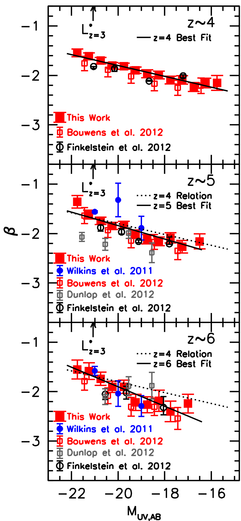
Figure 1.— Biweight-mean observed $\beta$’s for our $z\sim 4$ (upper panel), $z\sim 5$ (middle panel), and $z\sim 6$ (lower panel) galaxy samples as a function of the rest-frame $UV$ luminosity $M_{UV}$ (see also Table 2 for the binned measurements). These samples take advantage of the deeper ACS+WFC3/IR observations over the XDF and also the wider-area CANDELS-North observations, in addition to the CANDELS-South, ERS, and HUDF-Ps observations that Bouwens et al. (2012) utilized. For context, the $\beta$ vs. $M_{UV}$ relations derived by Bouwens et al. (2012), Wilkins et al. (2011), Dunlop et al. (2012), and Finkelstein et al. (2012) are also shown. The median $\beta$’s we quote for Finkelstein et al. (2012) for the lowest luminosity $z\sim 4$ and $z\sim 5$ galaxies rely exclusively on their $\beta$ measurements from the HUDF. While Finkelstein et al. (2012) do not explicitly quote these median $\beta$’s in their paper, these median $\beta$’s can be extracted from the information provided and were previously presented in Figure 11 of Bouwens et al. (2012). The solid lines give the best-fit linear relationship to the mean $\beta$ vs. $M_{UV}$ relationship. The present determination of this relationship is in excellent agreement with those previously derived by Bouwens et al. (2012), albeit with a slight offset to the intercept consistent with the estimated systematic errors (§3.3).

3. Lower Redshift $\beta$ Results as a Baseline for Interpreting $z>6$ Results

3.1. $z\sim 4$-6 Samples: Source Selection and $\beta$ Measurements

Previously, Bouwens et al. (2012) made use of the substantial quantity of observations over the HUDF09, ERS, and CANDELS-South fields to conduct a thorough characterization of the $\beta$ distribution over a wide luminosity range for star-forming galaxies at $z\sim 4$, $z\sim 5$, and $z\sim 6$. The availability of even deeper near-IR observations over the HUDF region (provided by the XDF data set) and observations over the CANDELS-North field allow us to further refine this characterization. An improved measurement of the $\beta$ distribution for faint galaxies at $z\sim 4$-6 will also be useful for establishing the approximate evolution in $\beta$ versus redshift and therefore interpreting the $\beta$ results for faint galaxies at $z\sim 7$-8 (§3.5).

We select our $z\sim 4$-6 samples slightly differently for the deeper and shallower datasets. First, we consider the $z\sim 4$-6 sample selection for the shallower, wide-area datasets, i.e., the CANDELS-North, CANDELS-South, or ERS data sets. The selection criteria we utilize are identical to what we previously utilized in Bouwens et al. (2012). These criteria are

$$(B_{435}-V_{606}>1.1)\wedge(B_{435}-V_{606}>(V_{606}-z_{850})+1.1)$$

$$\wedge(V_{606}-z_{850}<1.6)$$

for our $z\sim 4$ sample,

$$[(V_{606}-i_{775}>0.9(i_{775}-z_{850})+1.5)\vee$$

$$(V_{606}-i_{775}>2))]\wedge$$

$$(V_{606}-i_{775}>1.2)\wedge(i_{775}-z_{850}<0.8)$$

for our $z\sim 5$ selection, and

$$(i_{775}-z_{850}>1.3)\wedge(z_{850}-J_{125}<0.9)$$

where $\wedge$ and $\vee$ represent the logical AND and OR symbols, respectively. Sources in our $z\sim 5$ selections must be detected at less than $2\sigma$ in the $B_{435}$-band observations. Similarly, we require that sources in our $z\sim 6$ selections be undetected at $2\sigma$ in the $B_{435}$-band observations and that the sources be either undetected in the $V_{606}$-band observations or have a $V_{606}-z_{850}$ color redder than 2.8 (identical to the criteria utilized by Bouwens et al. 2006 in selecting $z\sim 6$ sources). Sources are required to be detected at $>$5.5$\sigma$ in the $\chi^{2}$ image we generated from the $Y_{105}J_{125}H_{160}$ imaging observations (or $Y_{098}J_{125}H_{160}$ imaging observations for our ERS samples).

Table 2The biweight mean, median, and inverse-variance-weighted mean $\beta$ for $z\sim 4$-8 galaxies, as a function of $UV$ luminosity $M_{UV}$

			Inverse-Variance
$<M_{UV,AB}>$	Biweight Mean $\beta$	Median $\beta$	Weighted Mean $\beta$	# of Sources
z$\,\sim\,$4 (§3.2)
$-$21.75	$-$1.54$\pm$0.07$\pm$0.06	$-$1.49${}_{-0.10}^{+0.08}$$\pm$0.06	$-$1.42$\pm$0.05$\pm$0.06	54
$-$21.25	$-$1.61$\pm$0.04$\pm$0.06	$-$1.61${}_{-0.05}^{+0.04}$$\pm$0.06	$-$1.52$\pm$0.03$\pm$0.06	141
$-$20.75	$-$1.70$\pm$0.03$\pm$0.06	$-$1.70${}_{-0.02}^{+0.07}$$\pm$0.06	$-$1.57$\pm$0.02$\pm$0.06	285
$-$20.25	$-$1.80$\pm$0.02$\pm$0.06	$-$1.81${}_{-0.03}^{+0.04}$$\pm$0.06	$-$1.71$\pm$0.02$\pm$0.06	457
$-$19.75	$-$1.81$\pm$0.03$\pm$0.06	$-$1.81${}_{-0.03}^{+0.04}$$\pm$0.06	$-$1.74$\pm$0.02$\pm$0.06	552
$-$19.25	$-$1.90$\pm$0.02$\pm$0.06	$-$1.88${}_{-0.02}^{+0.03}$$\pm$0.06	$-$1.85$\pm$0.02$\pm$0.06	586
$-$18.75	$-$1.97$\pm$0.06$\pm$0.06	$-$1.96${}_{-0.06}^{+0.05}$$\pm$0.06	$-$1.90$\pm$0.05$\pm$0.06	57
$-$18.25	$-$1.99$\pm$0.06$\pm$0.06	$-$1.98${}_{-0.09}^{+0.07}$$\pm$0.06	$-$1.97$\pm$0.05$\pm$0.06	70
$-$17.75	$-$2.09$\pm$0.08$\pm$0.06	$-$2.00${}_{-0.12}^{+0.06}$$\pm$0.06	$-$1.92$\pm$0.05$\pm$0.06	94
$-$17.25	$-$2.09$\pm$0.07$\pm$0.06	$-$2.07${}_{-0.08}^{+0.03}$$\pm$0.06	$-$2.04$\pm$0.06$\pm$0.06	69
$-$16.75	$-$2.23$\pm$0.10$\pm$0.06	$-$2.25${}_{-0.11}^{+0.07}$$\pm$0.06	$-$2.10$\pm$0.07$\pm$0.06	86
$-$16.25	$-$2.15$\pm$0.12$\pm$0.06	$-$2.19${}_{-0.10}^{+0.12}$$\pm$0.06	$-$1.94$\pm$0.08$\pm$0.06	96
$-$15.75	$-$2.15$\pm$0.12$\pm$0.06	$-$2.16${}_{-0.07}^{+0.12}$$\pm$0.06	$-$1.95$\pm$0.14$\pm$0.06	53
z$\,\sim\,$5 (§3.2)
$-$21.75	$-$1.36$\pm$0.48$\pm$0.06	$-$1.14${}_{-0.28}^{+0.61}$$\pm$0.06	$-$0.72$\pm$0.11$\pm$0.06	12
$-$21.25	$-$1.62$\pm$0.11$\pm$0.06	$-$1.55${}_{-0.11}^{+0.13}$$\pm$0.06	$-$1.44$\pm$0.07$\pm$0.06	35
$-$20.75	$-$1.74$\pm$0.05$\pm$0.06	$-$1.77${}_{-0.03}^{+0.07}$$\pm$0.06	$-$1.61$\pm$0.04$\pm$0.06	83
$-$20.25	$-$1.85$\pm$0.05$\pm$0.06	$-$1.88${}_{-0.02}^{+0.06}$$\pm$0.06	$-$1.75$\pm$0.04$\pm$0.06	134
$-$19.75	$-$1.82$\pm$0.04$\pm$0.06	$-$1.82${}_{-0.05}^{+0.05}$$\pm$0.06	$-$1.82$\pm$0.04$\pm$0.06	150
$-$19.25	$-$2.01$\pm$0.07$\pm$0.06	$-$2.00${}_{-0.04}^{+0.10}$$\pm$0.06	$-$1.99$\pm$0.06$\pm$0.06	72
$-$18.75	$-$2.12$\pm$0.10$\pm$0.06	$-$2.15${}_{-0.05}^{+0.12}$$\pm$0.06	$-$2.08$\pm$0.07$\pm$0.06	38
$-$18.25	$-$2.16$\pm$0.09$\pm$0.06	$-$2.19${}_{-0.10}^{+0.12}$$\pm$0.06	$-$2.08$\pm$0.07$\pm$0.06	58
$-$17.75	$-$2.09$\pm$0.10$\pm$0.06	$-$2.02${}_{-0.14}^{+0.07}$$\pm$0.06	$-$2.02$\pm$0.09$\pm$0.06	38
$-$17.25	$-$2.27$\pm$0.14$\pm$0.06	$-$2.26${}_{-0.12}^{+0.09}$$\pm$0.06	$-$2.33$\pm$0.11$\pm$0.06	31
$-$16.50	$-$2.16$\pm$0.17$\pm$0.06	$-$2.20${}_{-0.15}^{+0.12}$$\pm$0.06	$-$2.34$\pm$0.14$\pm$0.06	26
z$\,\sim\,$6 (§3.2)
$-$21.75	$-$1.55$\pm$0.17$\pm$0.08	$-$1.53${}_{-0.25}^{+0.18}$$\pm$0.08	$-$1.59$\pm$0.17$\pm$0.08	6
$-$21.25	$-$1.58$\pm$0.10$\pm$0.08	$-$1.55${}_{-0.15}^{+0.09}$$\pm$0.08	$-$1.60$\pm$0.15$\pm$0.08	10
$-$20.75	$-$1.74$\pm$0.10$\pm$0.08	$-$1.73${}_{-0.12}^{+0.06}$$\pm$0.08	$-$1.71$\pm$0.11$\pm$0.08	23
$-$20.25	$-$1.90$\pm$0.09$\pm$0.08	$-$1.88${}_{-0.07}^{+0.09}$$\pm$0.08	$-$1.81$\pm$0.08$\pm$0.08	53
$-$19.75	$-$1.90$\pm$0.13$\pm$0.08	$-$1.93${}_{-0.06}^{+0.14}$$\pm$0.08	$-$1.91$\pm$0.11$\pm$0.08	37
$-$19.25	$-$2.22$\pm$0.18$\pm$0.08	$-$2.17${}_{-0.22}^{+0.15}$$\pm$0.08	$-$2.24$\pm$0.14$\pm$0.08	12
$-$18.75	$-$2.26$\pm$0.14$\pm$0.08	$-$2.23${}_{-0.10}^{+0.10}$$\pm$0.08	$-$2.19$\pm$0.13$\pm$0.08	17
$-$18.25	$-$2.19$\pm$0.22$\pm$0.08	$-$2.12${}_{-0.08}^{+0.44}$$\pm$0.08	$-$2.07$\pm$0.19$\pm$0.08	11
$-$17.75	$-$2.40$\pm$0.30$\pm$0.08	$-$2.45${}_{-0.27}^{+0.55}$$\pm$0.08	$-$2.28$\pm$0.18$\pm$0.08	17
$-$17.00	$-$2.24$\pm$0.20$\pm$0.08	$-$2.25${}_{-0.18}^{+0.17}$$\pm$0.08	$-$2.19$\pm$0.16$\pm$0.08	25
z$\,\sim\,$7 (§4.7)
$-$21.25	$-$1.75$\pm$0.18$\pm$0.13	$-$1.74${}_{-0.12}^{+0.14}$$\pm$0.13	$-$1.67$\pm$0.10$\pm$0.13	26
$-$19.95	$-$1.89$\pm$0.13$\pm$0.13	$-$1.88${}_{-0.08}^{+0.07}$$\pm$0.13	$-$1.86$\pm$0.08$\pm$0.13	102
$-$18.65	$-$2.30$\pm$0.18$\pm$0.13	$-$2.66${}_{-0.08}^{+0.20}$$\pm$0.13	$-$2.39$\pm$0.14$\pm$0.13	43
$-$17.35	$-$2.42$\pm$0.28$\pm$0.13	$-$2.15${}_{-0.21}^{+0.17}$$\pm$0.13	$-$2.39$\pm$0.39$\pm$0.13	13
z$\,\sim\,$8 (§6.2)
$-$19.95	$-$2.30$\pm$0.01$\pm$0.27	$-$2.30${}_{-0.01}^{+0.01}$$\pm$0.27	$-$2.30$\pm$0.54$\pm$0.27	2
$-$18.65	$-$1.41$\pm$0.60$\pm$0.27	$-$1.51${}_{-1.07}^{+0.14}$$\pm$0.27	$-$1.88$\pm$0.74$\pm$0.27	4
z$\,\sim\,$8.5 (§6.3)
$-$18.50	$-$2.06$\pm$0.51$\pm$0.27	$-$1.82${}_{-0.73}^{+0.73}$$\pm$0.27	$-$2.07$\pm$0.92$\pm$0.27	2

The catalogs we utilize, in applying the above criteria, were derived purely from the optical/ACS $B_{435}V_{606}i_{775}I_{814}z_{850}$ observations (PSF-matched to the $z_{850}$ band) where possible. This ensures that the color measurements we use to select our $z\sim 4$-6 samples have very high S/N.

Second, we consider source selection over our deepest data sets, i.e., XDF, HUDF09-1, and HUDF09-2. We have revised the criteria we utilize from our shallower data sets. This was necessary to ensure that source selection is entirely decoupled from the measurement of $\beta$, so that we can obtain an unbiased measurement of $\beta$ to the limit of our $z\sim 4$-6 XDF+HUDF09-Ps samples. A coupling of source selection with the measurement of $\beta$ was an issue with previous $z\sim 7$ samples (Bouwens et al. 2010: see Appendix B.2), and so we must take special care to avoid it here (see Dunlop et al. 2012; Bouwens et al. 2012).

The selection criteria we settled upon for our deeper fields are

$$(B_{435}-V_{606}>1.1)\wedge(V_{606}-Y_{105}<1.3)\wedge$$

$$(V_{606}-z_{850}<1.6)$$

for our $z\sim 4$ sample,

$$(V_{606}-i_{775}>1.2)\wedge(i_{775}-J_{125}<0.9)$$

for our $z\sim 5$ selection, and

$$(i_{775}-z_{850}>1.0)\wedge(z_{850}-J_{125}<0.5)$$

for our $z\sim 6$ selection. When applying color criteria involving only ACS observations, smaller-aperture color measurements (PSF-matched to the $z_{850}$-band data) were utilized on special 0.03^′′-reductions generated for the XDF, HUDF09-1, and HUDF09-2 data sets to ensure more optimal results.

Source selection and photometry for our $z\sim 4$, $z\sim 5$, and $z\sim 6$ samples is based on the square root of $\chi^{2}$ image (Szalay et al. 1999) constructed from the $V_{606}Y_{105}JH_{140}H_{160}$-band, $J_{125}JH_{140}$-band, and $J_{125}JH_{140}$-band images, respectively. The $Y_{105}$ or $H_{160}$ band images were not used in constructing the $\chi^{2}$ image for our $z\sim 5$ and $z\sim 6$ samples (or the $J_{125}$-band image for our $z\sim 4$ samples), given our use of these images to derive $\beta$. Sources are required to be detected at $5\sigma$ in the $\chi^{2}$ image to ensure that they are real.

Using the same simulations as provided in Appendix F, we verified that the above selection criteria resulted in very similar mean redshifts for our $z\sim 4$, $z\sim 5$, and $z\sim 6$ selections from the deep XDF+HUDF09-Ps data sets as for our shallower ERS+CANDELS selections since the respective selection criteria differed only slightly. The mean redshifts we found for $z\sim 5$ and $z\sim 6$ for both selections were identically equal to 5.0 and 5.9, respectively, while for our $z\sim 4$ selections, the mean redshifts were equal to 3.8 (for our ERS+CANDELS selections) and 4.0 (for our XDF+HUDF09-Ps selection).

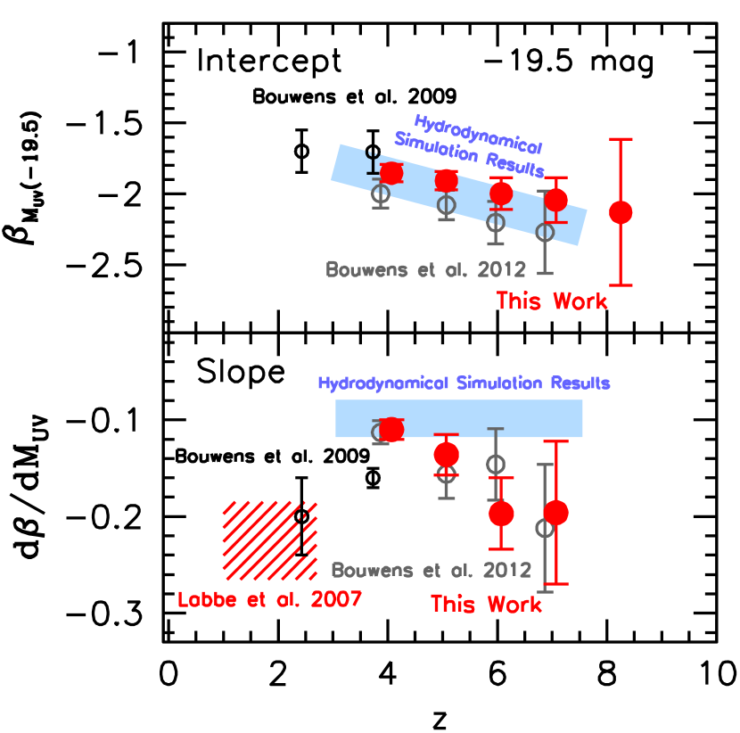
Figure 2.— Slope and Intercept of the $\beta$-$M_{UV}$ color-luminosity relationship for star-forming galaxies at various redshifts (see also Table 3). (Upper Panel) Intercept of the $\beta$-$M_{UV}$ color-luminosity relationship at a fixed $UV$ luminosity ($M_{UV}$) of $-19.5$ AB mag. The present determination is shown with the large red circles, while our earlier determinations at $z\sim 2.5$-4 and $z\sim 4$-6 (Bouwens et al. 2009; Bouwens et al. 2012) are shown with smaller open black circles and gray circles. The mean $\beta$ derived at fixed luminosity ($M_{UV,AB}=-19.5$) shows some reddening with cosmic time, but the evolution is not large. The derived trend is in remarkably good agreement with the predictions of the hydrodynamical simulations from Finlator et al. (2011: light blue shaded region). (Lower Panel) Slope of the $\beta$-$M_{UV}$ color-luminosity relationship. This relation is such that brighter galaxies exhibit redder $\beta$’s than fainter galaxies. The symbols are as in the upper panel. The slope to this relation at $z\sim 1.0$-2.7, as inferred by Labbé et al. 2007, is also shown with the red cross-hatched region (see Figure 7 from Bouwens et al. 2012). The slope of the $\beta$-$M_{UV}$ relation does not show statistically significant evolution with cosmic time (see also Bouwens et al. 2012).

The total number of sources that satisfied our $z\sim 4$, $z\sim 5$, and $z\sim 6$ criteria were 2925, 670, and 210, respectively. $\beta$’s are derived for individual sources in our $z\sim 4$, $z\sim 5$, and $z\sim 6$ samples using the same power-law fits ($f_{\lambda}\propto\lambda^{\beta}$) used for our $z\sim 7$ samples (see also Bouwens et al. 2012). For sources in the ERS, CANDELS-North, and CANDELS-South fields, $\beta$’s are then derived for $z\sim 4$, $z\sim 5$, and $z\sim 6$ galaxies from power-law fits to the photometry in the $i_{775}I_{814}z_{850}Y_{105}J_{125}$, $z_{850}Y_{105}J_{125}H_{160}$, and $Y_{105}J_{125}H_{160}$ bands, respectively. Where available (e.g., over the ERS field), use of the $Y_{098}$-band photometry was made. All the photometry used for the $\beta$ determinations are PSF-matched to the $H_{160}$ band. By selecting sources using photometry in smaller (and different) apertures than the photometry we use to derive $\beta$, we are able to ensure that our $\beta$ are much more immune to noise-driven systematic biases, such as the photometric error coupling bias discussed in Appendix B.1.2 of Bouwens et al. (2012).

For sources in the deeper XDF, HUDF09-1, and HUDF09-2 data sets, the flux measurements are made in the $i_{775}I_{814}z_{850}J_{125}$ bands for our $z\sim 4$ sample, in the $z_{850}Y_{105}H_{160}$ bands for our $z\sim 5$ sample, and in the $Y_{105}H_{160}$ bands for our $z\sim 6$ sample. We restrict our fits to these bands to ensure that there is no coupling between the selection of sources and the determination of $\beta$, therefore ensuring that noise-driven biases are identically zero. Similar to our procedure on our shallower data sets, all the photometry used for the $\beta$ determinations are performed from images PSF-matched to the $H_{160}$ band.

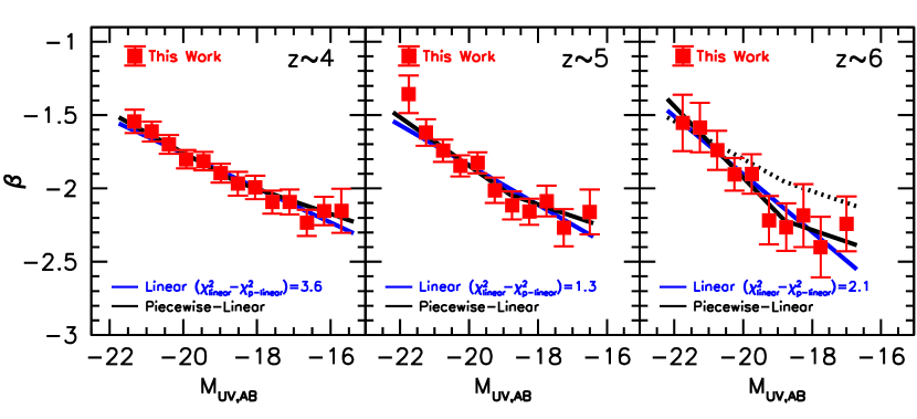
Figure 3.— Comparison of simple linear (blue lines) and piecewise-linear fits (black lines) to our $z\sim 4$ (left), $z\sim 5$ (center), $z\sim 6$ (right panels) $\beta$ vs. $M_{UV}$ results (see §3.4). Our piecewise-linear fits are made over two linear segments, with the slope of the faint piece fixed to $d\beta/dM_{UV}=-0.08$. For simplicity, we have kept the break luminosity fixed in our piecewise-linear models to the average best-fit break luminosity found at $z\sim 4$, $z\sim 5$, and $z\sim 6$, which is $-18.8\pm 0.2$ mag. The slope that we use faintward of the break luminosity $d\beta/dM_{UV}$ is taken to be equal the average best-fit slope we found for our $\beta$ results at $z\sim 4$, $z\sim 5$, and $z\sim 6$ (when allowing this slope to vary). The best-fit parameters we find for our piecewise-linear model are given in Table 4. The reduced $\chi^{2}$ values we compute with our piecewise-linear models provide a significantly better fit to the observed $\beta$ vs. $M_{UV}$ relationship than simple linear fits (96%, 75%, and 85% confidence at $z\sim 4$, $z\sim 5$, and $z\sim 6$, respectively). The present fit results suggest that the mean $\beta$’s for galaxies at very low luminosities, i.e., $M_{UV,AB}>-19$, show a weaker dependence on $UV$ luminosity than at higher luminosities. This result is strikingly similar to the $z\sim 4$ results of Oesch et al. (2013a) who also found that $\beta$ showed a steep dependence on the rest-frame optical luminosity for the most luminous galaxies and then a dramatic flattening to this relationship at lower luminosities. Comparing the best-fit results at $z\sim 4$ (dotted black line in right panel) with those at $z\sim 6$, we see clear evidence for evolution in the mean $\beta$’s for faint ($M_{UV,AB}>-18.8$) galaxies (see also Figure 4).

We bin galaxies as a function of their rest-frame $UV$ luminosity, as we did for our $z\sim 7$ samples. We take the $UV$ luminosity to be equal to the geometric mean of the magnitude measurements used to derive $\beta$ to minimize the effect of noise in introducing an artificial correlation between $\beta$ and $UV$ luminosity, as we did in Bouwens et al. (2009) and Bouwens et al. (2012). To ensure that our prescription for deriving the $UV$ luminosity did not substantially bias our $\beta$ results, we also examined the $\beta$ vs. $UV$ luminosity results defining the $UV$ luminosity in terms of the flux in bands used to select the sources, i.e., the $Y_{105}$-band flux for $z\sim 4$ sources and the $J_{125}$ or $J_{125}+JH_{140}$ flux for sources in our $z\sim 5$-6 samples. The results are briefly presented in Appendix E; we find no significant differences relative to our primary results.

In mapping out the mean $\beta$ versus $M_{UV}$ relationship, it is important to have a sufficient number of sources in each luminosity bin to determine the mean given the considerable scatter in the intrinsic $\beta$ distribution (Bouwens et al. 2009, 2012; Castellano et al. 2012; Rogers et al. 2014). We therefore rely on our CANDELS+ERS samples brightward of $-19$ mag and XDF/HUDF09-Ps samples faintward of these limits. Similar to the exercise shown in Figure 25 of Bouwens et al. (2012), we carefully compared the $\beta$’s derived from the deeper data sets with the shallower data sets to ensure that no large systematics are present between our data sets.

3.2. $\beta$ Results for $z\sim 4$-6 Samples

Our biweight mean $\beta$ results for our $z\sim 4$, $z\sim 5$, and $z\sim 6$ samples are presented in Figure 1 and Table 2. Very small ($\Delta\beta\sim 0.01$, $\Delta\beta\sim 0.02$, and $\Delta\beta\sim 0.01$) redward corrections were made to our biweight mean, median, and inverse-variance-weighted mean $\beta$ results at $z\sim 4$, $z\sim 5$, and $z\sim 6$, respectively, to correct for the fact that our color criteria are less efficient at selecting sources with intrinsically red $\beta$’s (see Appendix F). We also made a small ($\Delta\beta\sim 0.02$) blueward correction to $z\sim 5$ $\beta$ results from our wide-area ERS+CANDELS samples to correct for a slight coupling bias between our ERS+CANDELS $z\sim 5$ selections and the $\beta$ measurements we make in these data sets (see Appendix B.1.2 of Bouwens et al. 2012 for a description of the relevant simulations).

Current constraints on the mean $\beta$’s of galaxies extend to an unprecedented $-15.5$ mag at $z\sim 4$, $-16.5$ mag at $z\sim 5$, and $-17.0$ mag at $z\sim 6$ thanks to the superb depth of the optical+near-IR observations over our XDF data set. Median and inverse-variance-weighted mean $\beta$ are also provided for our $z\sim 4$-6 samples in Table 2, as a function of $UV$ luminosity. For context, the recent results of Bouwens et al. (2012), Wilkins et al. (2011), Dunlop et al. (2012), and Finkelstein et al. (2012) are also included in Figure 1.

Based on our $\beta$ results for our galaxy samples at $z\sim 4$, $z\sim 5$, and $z\sim 6$, we present the best-fit slope and intercept to the $\beta$ vs. $M_{UV}$ relationship in Figure 2 and Table 3. In Figure 2, we compare the observed trends with our new $\beta$ results at $z\sim 7$ (§4), the $\beta$ results at $z\sim 1$-6 from the literature (Labbé et al. 2007; Bouwens et al. 2009; Bouwens et al. 2012), and also with the hydrodynamical simulation results from Finlator et al. (2011). Encouragingly enough, almost identical trends are found between $\beta$ and $UV$ luminosity in large cosmological hydrodynamical simulations (e.g., Finlator et al. 2011).

The observed correlation of $\beta$ with luminosity is found to be even stronger when viewed at rest-frame optical wavelengths with Spitzer/IRAC (Oesch et al. 2013a). This is likely a manifestation of the well-known mass-metallicity relation (e.g., Tremonti et al. 2004; Erb et al. 2006a; Maiolino et al. 2008) in galaxies at $z\gtrsim 4$, with $UV$ luminosity roughly tracing with mass and $\beta$ tracing dust extinction and metallicity (Meurer et al. 1999; Bouwens et al. 2009; Bouwens et al. 2012).

Table 3The Best-Fit Slope and Intercept of $\beta$ - $M_{UV}$ color-luminosity relationship (see also Figure 2).

Sample	$<z>$	$\beta_{M_{UV}}=-19.5$	$d\beta/dM_{UV}$	Ref
$U_{300}$	2.5	$-1.70\pm 0.07\pm 0.15$	$-0.20\pm 0.04$	[1]
$B_{435}$	3.8	$-1.85\pm 0.01\pm 0.06$	$-0.11\pm 0.01$	[2]
$V_{606}$	5.0	$-1.91\pm 0.02\pm 0.06$	$-0.14\pm 0.02$	[2]
$i_{775}$	5.9	$-2.00\pm 0.05\pm 0.08$	$-0.20\pm 0.04$	[2]
$z_{850}$	7.0	$-2.05\pm 0.09\pm 0.13$	$-0.20\pm 0.07$	[2]
$Y_{105}$	8.0	$-2.13\pm 0.44\pm 0.27$	$-0.15$ (fixed)	[2]

Table 4The Best-Fit Slope and Intercept to $\beta$ - $M_{UV}$ color-luminosity relationship derived here using our piecewise-linear fits (see also Figure 3 and §3.4).

Sample	$<z>$	$\beta_{M_{UV}}=-18.8$	$d\beta/dM_{UV}$
$B_{435}$	3.8	$-1.95\pm 0.03\pm 0.06$	$-0.13\pm 0.02$
$V_{606}$	5.0	$-2.05\pm 0.05\pm 0.06$	$-0.17\pm 0.04$
$i_{775}$	5.9	$-2.22\pm 0.12\pm 0.08$	$-0.24\pm 0.07$

We also include our $z\sim 8$ results from §6, though we note that they are quite uncertain and do not provide a useful constraint. Consistent with our previous findings (Bouwens et al. 2009, 2012), we observe a similar slope to the $\beta$-$M_{UV}$ relationship at all redshifts under examination, with the most luminous galaxies being the reddest while the lowest luminosity galaxies are generally the bluest (as shown directly in Figure 1).

3.3. Comparison with Previous Results

As can be seen in Figure 1, the new $\beta$ determinations and those in the literature are broadly consistent (Wilkins et al. 2011; Bouwens et al. 2012; Finkelstein et al. 2012; Dunlop et al. 2012). The Dunlop et al. (2012) $z\sim 5$ $\beta$ determinations are clearly quite a bit bluer for the highest luminosity galaxies, but Dunlop et al. (2012) do not likely probe sufficient area with their study to include a statistically representative number of the reddest, high luminosity galaxies at $z\sim 5$.

The strong correlation we observe between $\beta$ and $UV$ luminosity is in excellent agreement with what was previously found in Bouwens et al. (2012: see also Bouwens et al. 2009), Wilkins et al. (2011) and Finkelstein et al. (2012: using their HUDF measurements to define the $\beta$ dependence to lower luminosities).

Figure 4.— The biweight mean $UV$-continuum slope $\beta$ observed for faint galaxies in our XDF + HUDF09-Ps $z\sim 4$, $z\sim 5$, $z\sim 6$, $z\sim 7$, and $z\sim 8$ samples (red solid circles). Only sources in the luminosity range $-19.0<M_{UV,AB}<-17.0$ are included in computing the means for the $z\sim 4$, $z\sim 5$, and $z\sim 6$ samples. For our $z\sim 7$ selection, sources in the somewhat more extended luminosity range $-19.3<M_{UV,AB}<-16.7$ are considered (to increase the signal-to-noise on our measurement somewhat). $1\sigma$ uncertainties on each of the determinations are also shown, for the statistical uncertainties alone (including hashes at the ends) and including the systematic uncertainties (not including hashes). The $z\sim 8$ results that are presented are based on an extrapolation of the $\beta$-$M_{UV}$ relationship that we determine (see Table 3). The blue open circles show our biweight mean $\beta$ determinations from the XDF data set alone. The expectations from hydrodynamical simulations (Finlator et al. 2011) are shown for comparison with the thick light-blue line. $\gtrsim$60% of the evolution in $\beta$ in the Finlator et al. (2011) simulations occurs due to changes in the dust extinction (Bouwens et al. 2012; Finkelstein et al. 2012).

Nevertheless, we do note a clear offset in the $\beta$ vs. $M_{UV}$ relationship relative to what we reported earlier in Bouwens et al. (2012). At fixed luminosity and redshift, the $\beta$’s we find are systematically redder by $\Delta\beta\sim 0.13$-0.19. While our new results are consistent with our older results given the large systematic uncertainties we quoted on the derive $\beta$’s (Bouwens et al. 2012), the present results do represent a modest shift in our best-fit $\beta$ determinations. In general, this shift brings our derived $\beta$ measurements into better agreement with other determinations in the literature (Figure 1).

The offset in the $\beta$ vs. $M_{UV}$ relationship arises from the systematically redder $\beta$’s ($\Delta\beta\sim 0.10$-0.15) we measure at all redshifts. As we explain in Appendix B.3, this occurred due to the empirical PSFs from Bouwens et al. (2012) not containing sufficient light on the wings. As a result, during the PSF-matching process, light in the bluer bands was not sufficiently smoothed to match the $H_{160}$-band PSF. This resulted in a systematic bias towards bluer $\beta$’s at all redshifts. Other potentially contributing factors are (1) the fact that the mean $\beta$’s we measure for bright galaxies in the CANDELS-North field are slightly redder ($\Delta\beta\sim 0.05$) in the mean than what we measure over the CANDELS-South and (2) the corrections that Bouwens et al. (2012) performed to remove the photometric error coupling bias appear to have been too large (although these corrections had a size of just $\Delta\beta\sim 0.025$ to $\Delta\beta\sim 0.05$). The latter issue is no longer a concern for the present analysis, since we have constructed our faint samples such that the photometric error coupling bias is identically zero (see §3.1 and §4.2).

3.4. Evidence for a Much Weaker Dependence of $\beta$ on $UV$ Luminosity for Faint $z\sim 4$-6 Galaxies?

The superb depth of the optical+near-IR observations and improved techniques allow us to study the $UV$ slopes $\beta$ of faint $z\geq 4$ galaxies at even lower luminosities than in previous work, reaching to $-15.5$ mag ($0.006L_{z=3}^{*}$) at $z\sim 4$, $-16.5$ mag ($0.014L_{z=3}^{*}$) at $z\sim 5$, and $-17.0$ mag ($0.025L_{z=3}^{*}$) at $z\sim 7$. Key questions for these faint galaxy samples include what is the mean $\beta$ and how does $\beta$ depend on $UV$ luminosity (and therefore likely mass).

In our previous work and in §3.2, we modeled the dependence of $\beta$ on $UV$ luminosity using a simple two-parameter linear relationship. Such a model was required to capture the clear trend in the mean $\beta$’s from very red values for the highest luminosity systems to very blue values at lower luminosities. As Figure 1 illustrates, a simple linear relation largely captures the observed trends in $\beta$ with $UV$ luminosity.

However, looking at the relationship between the observed $\beta$’s and $M_{UV}$ more closely, we can see clear evidence for deviations from such a simple linear relationship. In particular, brightward of $-19$ mag, the mean $\beta$’s show a strong dependence on the $UV$ luminosity, while faintward of $\sim-19$ mag, these $\beta$’s show almost no dependence on the luminosity. This is illustrated in Figure 3. Oesch et al. (2013a) have already observed a similar behavior in $\beta$ as a function of luminosity, but at rest-frame optical wavelengths.

Based on simple physical considerations, we might expect such a dependence of $\beta$ on $UV$ luminosity if the dust extinction in galaxies shows a significant correlation with the mass or the luminosity of galaxies, and indeed such has been shown (e.g., Figure 18 from Reddy et al. 2010 and Figure 5 from Pannella et al. 2009). For galaxies where the luminosities or dust extinction is large, modest changes in luminosity (or dust extinction) would have a large impact on $\beta$. For galaxies where the $UV$ luminosity or dust extinction is smaller, the impact would be much less. The theoretical predictions of Dayal et al. (2013) also suggest only a mild dependence of $\beta$ on luminosity in this regime, though at sufficiently low luminosities Dayal et al. (2013) predict somewhat bluer $\beta$’s (e.g., $\beta\sim-2.5$).

One way of attempting to model the observed $\beta$’s given this situation is to use a piecewise-linear model, where we allow for a different dependence on the $UV$ luminosity brightward of some break than faintward of this break. Utilizing such a four-parameter model (adding some break luminosity and slope faintward of the break to standard two-parameters linear fits), we recover $-19.0\pm 0.4$ mag, $-18.8\pm 0.2$ mag, and $-18.8\pm 0.8$ mag for the break luminosity at $z\sim 4$, $z\sim 5$ and $z\sim 6$, respectively, and find a best-fit $d\beta/dM_{UV}$ dependence of $-$0.08$\pm$0.03, $-$0.08$\pm$0.07, $-$0.02$\pm$0.17, respectively, faintward of this break luminosity. Almost identical break luminosities (i.e., $-19.3$ to $-18.8$) are found fitting only to our binned $\beta$ results from the XDF and HUDF09-Ps data sets, so the position of this break is not an artifact of some offset between the wide and deep field $\beta$’s and our only making use of wide-area samples brightward of $-19$ mag. It is remarkable how similar our results are for break luminosities and faint-end slopes at all redshifts, suggesting that the break luminosity we uncovered has a fundamental physical origin.

It is interesting to compare the reduced $\chi^{2}$’s we derive from these piecewise-linear fits with those obtained using simple fits to a line. For the piecewise-linear fits, we fix the break luminosity to $-18.8$ (the average break luminosity we find at $z\sim 4$, $z\sim 5$, and $z\sim 6$) and the $d\beta/dM_{UV}$ slope faintward of this luminosity to $-0.08$ (the average slope faintward of the break for our $z\sim 4$, $z\sim 5$, and $z\sim 6$ samples). This reduces the dimensionality from four ($\beta$ intercept, break luminosity, slope brightward of the luminosity break, slope faintward of the break) to two ($\beta$ intercept, slope brightward of the luminosity break). For this two-parameter piecewise linear model, we find best-fit $\chi^{2}$’s that are $\Delta\chi^{2}$ $=\,$3.6, 1.3, and 2.1 lower than the equivalent linear fits in representing our $z\sim 4$, $z\sim 5$, and $z\sim 6$ $\beta$ vs. $M_{UV}$ determinations, respectively. These two models for representing the observed $\beta$ vs. $M_{UV}$ relationship are shown in Figure 3. The best-fit parameters we find for our piecewise-linear model (with fixed faint-end slope and break luminosity) are provided in Table 4. Based on the differences in $\chi^{2}$ values for these two-parameter models, it is clear that our piecewise-linear model (with only a weak dependence on $UV$ luminosity faintward of $-19$ mag) provides a noticeably superior representation for the observed $\beta$ vs. $M_{UV}$ relationship at $z\sim 4$, $z\sim 5$ and $z\sim 6$ (96%, 75%, and 85% confidence, respectively).

3.5. Extrapolating $\beta$ Results from Faint Galaxies at $z\sim 4$-6 to Higher Redshifts

As Figure 1 illustrates, the mean $UV$-continuum slopes $\beta$ for $z\sim 4$, $z\sim 5$, and $z\sim 6$ galaxies are now quite well established on the basis of current observations and exhibit a similar dependence on $UV$ luminosity independent of redshift (see also Figure 2). This dependence on $UV$ luminosity is likely weaker faintward of $-19$ mag for galaxies at all redshifts under consideration here (Figure 3). The quality of the $z\sim 4$-6 constraints directly follows from the much larger sample sizes available at these redshifts, the substantial wavelength leverage available to constrain $\beta$ for individual sources, and the superb depth of data sets like the XDF.

The $z\sim 4$-6 $\beta$ results provide us with a solid baseline on which to establish expectations for the $\beta$ distribution at even higher redshifts. An important question from the previous sections regards the mean value of $\beta$ for lower-luminosity galaxies in the $z\sim 7$-8 universe. For our $z\sim 4$, $z\sim 5$, and $z\sim 6$ samples, we can set strong constraints on the mean $\beta$’s using existing observations. In Figure 4, we present the biweight mean $\beta$’s we derive as a function of redshift from $z\sim 4$, $z\sim 5$, and $z\sim 6$ XDF+HUDF09-Ps samples.

Only galaxies in the luminosity range $-19<M_{UV,AB}<-17$ are considered in these comparisons for our $z\sim 4$-6 samples. Also shown on Figure 4 are the expectations from the hydrodynamical simulations of Finlator et al. (2011). The best-fit trend we find at $z\gtrsim 4$ for the biweight mean $\beta$ for faint ($-19<M_{UV,AB}<-17$) galaxies is $-2.14\pm 0.06-(0.10\pm 0.06)(z-4.9)$. Here we include in our error budget both the statistical errors and our conservative systematic error estimates. Extrapolating the results from our $z\sim 4$-6 samples to $z>6$, we predict the mean $\beta$ for lower-luminosity galaxies at $z\sim 7$ and $z\sim 8$ to be $-2.35\pm 0.16$ and $-2.45\pm 0.23$, respectively (conservatively accounting for possible systematic errors on our $\beta$ determinations). The mean $\beta$’s we derive for faint $z\sim 7$-8 galaxies in §4 and §6 are in excellent agreement with these extrapolations.

Table 5Filters used to measure $\beta$ for $z\sim 7$ galaxies (approximate orbit totals in parentheses).

	Source Detection and Selection
	Color Redward of Break		Contributes to	$\beta$ Measurement
Field	Blue Anchor	Red Anchor	Detection Image	Blue Anchor	Central Anchor	Red Anchor
XDF	$Y_{105}$ (100)	$J_{125,1}$ (20)	$H_{160,1}$ (43)	$J_{125,2}$ (20)	$JH_{140}$ (30)	$H_{160,2}$ (42)
	$Y_{105}$ (100)	$J_{125,2}$ (20)	$H_{160,2}$ (42)	$J_{125,1}$ (20)	$JH_{140}$ (30)	$H_{160,1}$ (43)
HUDF09-1	$Y_{105}$ (8)	$J_{125,1}$ (6)	$H_{160,1}$ (7)	$J_{125,2}$ (6)	—	$H_{160,2}$ (6)
	$Y_{105}$ (8)	$J_{125,2}$ (6)	$H_{160,2}$ (7)	$J_{125,1}$ (6)	—	$H_{160,1}$ (7)
HUDF09-2	$Y_{105}$ (11)	$J_{125,1}$ (9)	$H_{160,1}$ (10)	$J_{125,2}$ (9)	—	$H_{160,2}$ (9)
	$Y_{105}$ (11)	$J_{125,2}$ (9)	$H_{160,2}$ (9)	$J_{125,1}$ (9)	—	$H_{160,1}$ (10)
CANDELS	$Y_{105}$ (3)	$J_{125,1}$ (2)	$H_{160,1}$ (2)	$J_{125,2}$ (2)	—	$H_{160,2}$ (2)
	$Y_{105}$ (3)	$J_{125,2}$ (2)	$H_{160,2}$ (2)	$J_{125,1}$ (2)	—	$H_{160,1}$ (2)
ERS	$Y_{098}$ (2)	$J_{125,1}$ (1)	$H_{160,1}$ (1)	$J_{125,2}$ (1)	—	$H_{160,2}$ (1)
	$Y_{098}$ (2)	$J_{125,2}$ (1)	$H_{160,2}$ (1)	$J_{125,1}$ (1)	—	$H_{160,1}$ (1)

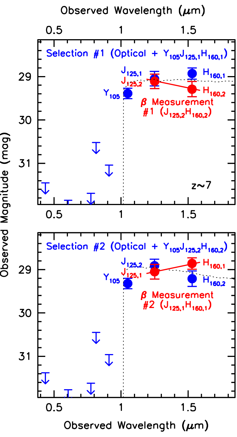
Figure 5.— (upper) An illustration of the information we use for selecting $z\sim 7$ sources from our fields and measuring $\beta$. The fluxes and $1\sigma$ uncertainties we derive for a $z\sim 7$ galaxy in the XDF. Two separate flux measurements are derived for this source at both $1.25\mu$m and $1.6\mu$m, from the two $\sim$50% splits of the $J_{125}$ and $H_{160}$-band exposures for this field (i.e., $J_{125,1}$, $J_{125,2}$, $H_{160,1}$, and $H_{160,2}$). Of importance for the selection (blue circles and $1\sigma$ upper limits) are the optical observations, $Y_{105}$, and half of the $J_{125}$ and $H_{160}$ band observations – which allow us to demonstrate that the selected sources are real, show a sharp Lyman break in the spectrum across the $z_{850}$ and $Y_{105}$ bands, show absolutely no flux blueward of the break (in the $B_{435}V_{606}i_{775}$ data), and exhibit a blue color redward of the break (using the flux in the $Y_{105}$ band and the first half of the $J_{125}$-band observations). Of importance for the measurement of $\beta$ are the measured fluxes (red circles) in the other half of the $J_{125}$ and $H_{160}$-band observations. By clearly separating source selection from the measurement of $\beta$, we can be sure that our $\beta$ measurements remain unbiased to faint magnitudes. (lower) To make full use of the available $J_{125}$ and $H_{160}$-band observations to maximize the accuracy of our $\beta$ measurements, we also consider a second selection of $z\sim 7$ galaxies over each of our fields, but utilizing the second half of the $J_{125}$ and $H_{160}$-band observations for the selection and the first half of the $J_{125}$ and $H_{160}$-band observations for the measurement of $\beta$. The photometry we obtain for sources is consistent with that from our first selection (upper panel), but is nonetheless slightly different (due to the impact of noise on the derived apertures).

4. $\beta$ Results for $z\sim 7$ Samples

A key part of the discussion regarding $\beta$ measurements has concerned the extent to which $\beta$ measurements may or may not be subject to biases. While this question is not new (e.g., see Meurer et al. 1999; Figure 4 from Bouwens et al. 2009), essentially all studies of $\beta$ at high redshift have fallen short in some regard in their handling of systematic errors.

We begin this section with a brief motivation and summary of our procedure for obtaining a measurement of the $\beta$ distribution for $z\sim 7$ galaxies, over a wide range in $UV$ luminosity while remaining free of systematic errors (we use the word “bias” here for simplicity). We use the phrase “noise-driven biases” to describe systematic biases that result from the impact of noise on two or more coupled quantities (such as when the same noise fluctuations can affect both source selection and the measurement of $\beta$). Then, we describe our selection and measurement procedures for $z\sim 7$ galaxies and give our results.

4.1. Why Noise-Driven Systematic Biases are A Particular Concern for $\beta$ Measurements at $z\sim 7$

While there are many potentially important biases for determinations of the mean $\beta$, one of the most prominent sources of bias that has received much discussion recently regards the interplay between redshift selection and $\beta$ measurement (see Appendix B.1.2 of Bouwens et al. 2012 or Dunlop et al. 2012). Sizeable biases in the measured $\beta$’s can occur, if the same information is used to select galaxies as is used to measure their $UV$-continuum slopes $\beta$. Since sources with bluer observed colors (redward of an apparent Lyman break) are more readily identified as $z\sim 7$ galaxies than sources with redder observed colors, one would be biased towards selecting sources which also have the bluest-apparent $\beta$, if the high-redshift selection is performed in the conventional way.

To overcome this bias, we must ensure that the information we have on sources relevant to their selection as $z\sim 7$ galaxies (detection significance, color redward of the break) is completely independent of that required to measure the $UV$-continuum slope $\beta$. Accomplishing this, however, requires that we be able to define two colors redward of the break that are entirely independent of each other. This appears to be challenging for $z\sim 7$ sources, due to the availability of only three different near-IR passbands with deep observations in the typical legacy field. For example, only three near-IR bands are available with deep WFC3/IR coverage in public surveys like CANDELS (Grogin et al. 2011; Koekemoer et al. 2011), the Early Release Science (ERS) program (Windhorst et al. 2011), or the HUDF09 program (Bouwens et al. 2011). This challenge has prompted researchers to correct for this bias based on simulations (Bouwens et al. 2012; Finkelstein et al. 2012) or to argue that observations in a fourth WFC3/IR band (e.g., F140W) may be required to obtain unbiased measurements of $\beta$ at $z\sim 7$ (Rogers et al. 2013; Dunlop et al. 2012). While this latter approach, with more bands has merit, very few data sets have deep observations in so many filters, and restricting $z\sim 7$ $\beta$ studies to those that do would restrict our ability to build up maximally-sized samples over a wide range of luminosity.

4.2. Bias-Free Procedure for Deriving $\beta$ at $z\sim 7$

Fortunately, we have a way forward that allows for essentially bias-free measurements of $\beta$ for $z\sim 7$ samples using just the available three-band WFC3/IR imaging in the many public HST fields. Observations in a fourth WFC3/IR band are not required to obtain bias-free results for $\beta$. The approach is simply to construct two independent, equal-depth reductions of both the $J_{125}$ and $H_{160}$-band data by splitting the full dataset on each field in half. Each dataset consists of dithered images that are reduced using our standard WFC3/IR pipeline (e.g., as in Bouwens et al. 2011). The result is two independent $J_{125}$ and $H_{160}$-band images of comparable depth covering the same field, but with independent noise properties.

We use the reduced image from the first half of the $J_{125}$/$H_{160}$-band data set to do the $z\sim 7$ selection, while the reduced image of the second half of the $J_{125}$/$H_{160}$-band data set is used for the $\beta$ measurements. We then reverse the roles of the $\sim$50% splits of the $J_{125}$/$H_{160}$-band data set, so that the first half is used for the $\beta$ measurements and the second half is used for the $z\sim 7$ selection. Figure 5 illustrates the algorithm. Putting together the $\beta$ measurements from the two different selections on each field, we can derive the mean $\beta$ with comparable S/N to what we would achieve, had we made use of the full (unsplit) $J_{125}$ and $H_{160}$ data sets to derive $\beta$. Previously, we introduced a less sophisticated version of this approach in §4.8 of Bouwens et al. (2012), but had only used this as a simple cross check on the Bouwens et al. (2012) $z\sim 7$ results for faint galaxies. Here we have systematically applied this procedure across all data sets under study (HUDF/XDF, HUDF09-1, HUDF09-2, CANDELS-North, CANDELS-South, ERS).

This more sophisticated procedure explicitly ensures (by construction) that our derived $\beta$’s are completely robust against the photometric error coupling bias described by Dunlop et al. (2012) and also by Bouwens et al. (2012: Appendix B.1.2). The photometric error coupling bias is the term Bouwens et al. (2012) used to describe the noise-driven systematic bias in $\beta$ that occurs when the same noise fluctuation can have an effect on both the selectability of a source and its measured $\beta$. More details regarding this procedure are given in §4.5.

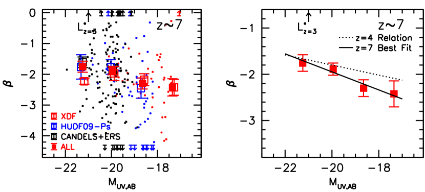
Figure 6.— (left) Measured $\beta$ of $z\sim 7$ galaxies in our XDF samples (red points), HUDF09-Ps samples (blue points), and ERS+CANDELS-S+CANDELS-North samples (black points). The points show sources at the average of the two $\beta$’s measured for an object if the same source is selected twice and at a source’s only $\beta$ determination if it is selected once. The large squares with $1\sigma$ error bars indicate the biweight mean $\beta$’s we measure in various $UV$ luminosity ($M_{UV}$) intervals from the XDF (red open squares), from the HUDF09-Ps (blue open squares), from the ERS+CANDELS-S+CANDELS-N (black open squares), and from our entire field set (red solid squares). The different determinations are slightly offset horizontally to improve the clarity of this figure. Error bars are derived from bootstrap resampling the $\beta$ results in each $UV$ luminosity interval. The biweight mean $\beta$’s that we derive from different data sets are generally in agreement to within their $1\sigma$ uncertainties, even at the detection limits of the shallowest ones. This suggests that our results are not substantially impacted by noise-driven systematic biases. These mean $\beta$’s are also presented in Table 2. (right) The mean $\beta$ we find in various $UV$ luminosity ($M_{UV}$) intervals (solid red squares). The solid black line indicates the best-fit linear relationship between $\beta$ and $UV$ luminosity ($M_{UV}$) for $z\sim 7$ galaxies, while the dotted line shows the relationship Bouwens et al. (2012) found for $z\sim 4$ star-forming galaxies. The relationship between $\beta$ and $UV$ luminosity exhibits a similar correlation at $z\sim 7$ as it exhibits at lower redshifts (see Figure 2).

4.3. Source Selection

Many different datasets are used for our selection of $z\sim 7$ galaxies to use in establishing $\beta$. As indicated in the previous section, we select $z\sim 7$ candidates from each of our data sets twice (see Table 5).

We base each of these selections on an independent photometric catalog we construct from each field. Object detection is performed on the basis of the square root of $\chi^{2}$ image generated from the $Y_{105}$, $J_{125}$, and $H_{160}$-band observations. For each catalog, we construct the $\chi^{2}$ image from the $\sim$50% $J_{125}$ and $H_{160}$-band stacks not utilized for the $\beta$ measurements. Photometry on the two $\sim$50% $J_{125}$-band stacks for a given field is carried out separately and kept completely separate throughout the selection and measurement process, as if the two stacks were flux measurements in different bands. An identical procedure is used for photometry on the two $\sim$50% stacks of the $H_{160}$-band observations. The reductions we use for our $z\sim 7$ $\beta$ determinations were done on a $0.06^{\prime\prime}$-pixel scale.

Redshift $z\sim 7$ galaxies are then selected from these catalogs using the same Lyman-break criteria we previously employed in Bouwens et al. (2012). For the XDF, HUDF09-Ps, and CANDELS fields (where we have $Y_{105}$-band data) the criteria we use are

$$(z_{850}-Y_{105}>0.7)\wedge(Y_{105}-J_{125}<0.8)\wedge$$

$$(z_{850}-Y_{105}>1.4(Y_{105}-J_{125})+0.42),$$

while for the ERS field the availability of only $Y_{098}$-band data lead us to use the criteria:

$$(z_{850}-J_{125}>0.9)\wedge~{}~{}~{}~{}~{}~{}~{}~{}~{}~{}~{}~{}$$

$$(z_{850}-J_{125}>0.4+1.1(Y_{098}-J_{125})).$$

When applying the above criteria, we set the fluxes of sources that are undetected to their $1\sigma$ upper limits. The $J_{125}$-band fluxes and images we utilize for these criteria are based on the $\sim$50% splits not utilized for the $\beta$ measurements (see Table 5). To ensure source reality, we require sources required to be detected at $5\sigma$, adding in quadrature the $Y_{105}$-band image with the 50% split of the $J_{125}$ and $H_{160}$-band exposures not used for the $\beta$ measurements. We also require sources are detected at $>4.3\sigma$ in the 50% splits of the $J_{125}$ and $H_{160}$-band exposures not used for the $\beta$ measurements. This is to ensure that the sources we use in deriving the mean $\beta$ have sufficient S/N that their $\beta$’s are well-defined (i.e., so the S/N of the F125W and F160W-band fluxes used to measure $\beta$ is not typically less than 1).

To minimize potential contamination from lower redshift interlopers, we require that sources in our selection show no detection ($<$2$\sigma$) in the $B_{435}$, $V_{606}$, or $i_{775}$ bands. To take advantage of the very deep $I_{814}$-band observations over the CANDELS fields (see e.g. Oesch et al. 2012 for a discussion), we require that sources be either undetected in the $I_{814}$-band in a given field ($<1\sigma$) or have a $I_{814}-Y_{105}$ band color $>$2 mag (or $I_{814}-Y_{098}>2$ mag for the ERS field).

Finally, we require the $\chi_{opt}^{2}$ statistic we construct for each source to be less than 3 for sources in the XDF, HUDF09-1, HUDF09-2, CANDELS, and ERS fields. The upper limits we set are similar but nonetheless slightly stronger in general than those adopted in Bouwens et al. (2011) and Bouwens et al. (2012). These limits allow us to select $z\gtrsim 7$ galaxies with minimal contamination ($\lesssim$10%).

As in Bouwens et al. (2011), we take the $\chi_{opt}^{2}$ statistic to be equal to $\Sigma_{i}SGN(f_{i})(f_{i}/\sigma_{i})^{2}$ where $f_{i}$ is the flux in band $i$, $\sigma_{i}$ is the flux error in band $i$, SGN($f_{i}$) is equal to 1 if $f_{i}>0$ and $-1$ if $f_{i}<0$, and where we consider the $B_{435}$, $V_{606}$, and $i_{775}$ bands in the sum. We apply the above $\chi^{2}$ criterion in three different apertures (0.18^′′-diameter apertures, small scalable apertures, and $0.35^{\prime\prime}$-diameter apertures) to ensure candidate $z\sim 7$ sources in our selection show no evidence for positive flux blueward of the break irrespective of morphology. We estimate that our contamination rates, while dependent on the field, are typically in the range $\sim$2% to 10% (see discussion in Bouwens et al. 2011 and Bouwens et al. 2014).

4.4. Methodology for Measuring $\beta$

In deriving $\beta$’s for our candidate sources, we use the same approach as in Bouwens et al. (2012: see also Castellano et al. 2012). Specifically, we fit the observed $J_{125}$-band and $H_{160}$-band fluxes to a power law $f_{\lambda}\propto\lambda^{\beta}$ to determine $\beta$. The effective wavelengths we use in performing the fit assume a flat $\beta\sim-2$ spectrum, and are 1243 nm, 1383 nm, 1532 nm for the $J_{125}$, $JH_{140}$, $H_{160}$. Given that the typical galaxy in our programs have $\beta$’s in the range $\beta\sim-1.5$ to $\beta\sim-2.5$, this is a somewhat better approximation than using the pivot wavelength $\lambda_{p}$ (Tokuanga & Vacca 2005) for this purpose. With the exception of the $z\sim 7$ sources over the HUDF – where fluxes are also available at $\sim$1.4$\mu$m from deep $JH_{140}$ data – only two flux measurements are used in this fit (i.e., $J_{125}$ and $H_{160}$). This approach therefore becomes equivalent to using the fitting formula

$$\beta=-2.0+4.39(J_{125}-H_{160}).$$ (1)

The 4.39 factor is 2% higher than the factor used in Bouwens et al. (2010) and 1% lower than advocated by Dunlop et al. (2012). The $J_{125}$-band fluxes that we use in these fits come from the $\sim$50% of the $J_{125}$-band observations not used in the selection of $z\sim 7$ candidates for a field (see §4.2 and Table 5).

In deriving $\beta$, we only make use of flux measurements which are clearly not affected by the IGM absorption or Ly$\alpha$ emission. Some studies (e.g., Finkelstein et al. 2012) have attempted to exploit the additional wavelength leverage provided by the $z_{850}$ and $Y_{105}$-band flux measurements to further improve their estimates of $\beta$. The difficulty with such approaches is their sensitivity to a number of potentially large (and unknown) systematics. Differences between the SED shapes or Ly$\alpha$ prevalence assumed versus that present in the real observations can have a significant impact on the results that cannot be readily quantified or appropriately corrected. This point is illustrated in Figure 12 of Rogers et al. (2013). Given this concern we do not make use of the $Y_{105}$-band flux for $z\sim 7$ candidates.

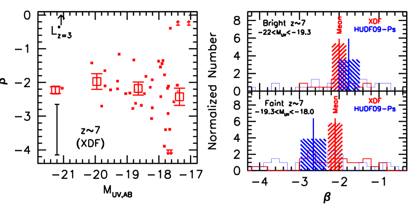
Figure 7.— (left panel) Measured $\beta$’s for $z\sim 7$ star-forming galaxy candidates in our XDF samples (small red squares). $1\sigma$ upper and lower limits are plotted for sources whose nominal $\beta$ measurements are redder than $-0.3$ or bluer than $-4.0$ (as one would expect for the lowest S/N sources in each data set). The error bar in the lower left-hand corner indicates the typical $1\sigma$ uncertainty on an individual $\beta$ determination in the luminosity range $-19.3<M_{UV,AB}<-18.0$. The large open red squares with $1\sigma$ error bars indicate the biweight mean $\beta$’s we measure in various $UV$ luminosity ($M_{UV}$) intervals from the XDF. As in previous studies (Labbé et al. 2007; Bouwens et al. 2009; Bouwens et al. 2010; Bouwens et al. 2012), our measurement of $\beta$ for galaxies in the XDF provide evidence that lower luminosity galaxies have bluer $\beta$’s. (upper right) The distribution of measured $UV$-continuum slopes $\beta$ for bright ($-22<M_{UV,AB}<-19.3$) $z\sim 7$ galaxies in the XDF (red histogram) and HUDF09-Ps (blue histogram) selections. While individual sources may appear as often as two times in each panel (due to our repeating our selection twice on each field), the number of sources in the two selections has been divided by two to give a realistic indication of the numbers of sources included in our $\beta$ estimates. The red vertical bar indicates the biweight mean $\beta$ for each luminosity subsample and the hashed region indicates the $1\sigma$ uncertainty. (lower right) Similar to the upper right panel, but for fainter ($-19.3<M_{UV,AB}<-18.0$) $z\sim 7$ sources over our fields. Clearly the fainter $z\sim 7$ sources have bluer $\beta$’s than the brighter sources.

4.5. Deriving a Bias-free Sample

As outlined in the introduction and at the beginning of this section, our procedure is to select sources from our fields twice, alternatively using the first and second half of the available $J_{125}$/$H_{160}$-band data in each field. Measurements of $\beta$ are made using the other half of the $J_{125}$/$H_{160}$-band observations not included in the $z\sim 7$ selection.

We systematically applied this procedure to all of the data sets and search fields considered in this study. The $\beta$’s we measure for candidate $z\sim 7$ galaxies in our fields are shown in Figure 6 as the blue, red, and black points.

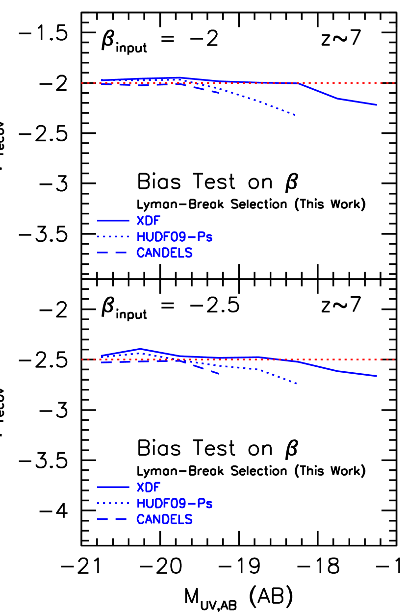
Figure 8.— The mean $\beta$’s we recover for a $z\sim 7$ galaxy population vs. the near-IR magnitude assuming an input $\beta$ of $-2$ (top) and $-2.5$ (bottom). Shown are the results for our $z\sim 7$ selections from the XDF (solid lines), the HUDF09-Ps fields (dotted lines), and the CANDELS-South/Deep region (dashed lines). The only source of bias in our recovered $\beta$’s is due to the fact that galaxies with bluer $\beta$’s are slightly easier to select than galaxies with redder $\beta$’s. This is the selection volume bias discussed in Appendix B.1.1 of Bouwens et al. (2012), and it affects both Lyman-Break (Bouwens et al. 2012; Wilkins et al. 2011) and photometric redshift selections (Dunlop et al. 2012; Finkelstein et al. 2012). Fortunately, the calculated selection volumes for our $z\sim 7$ samples from the XDF only exhibit a weak dependence on the input $\beta$’s, and therefore the expected bias is very small, i.e., $\Delta\beta\lesssim 0.03$ for galaxies with $UV$ luminosities brighter than $-18$ mag. Faintward of $-18$ mag, we expect a small bias in $\beta$ ($\sim$0.1-0.15). The other significant bias in $\beta$ is the photometric error coupling bias (described by Dunlop et al. (2012) and Bouwens et al. [2012: Appendix B.1.2]), but this bias is identically zero here, due to our using completely different information for selecting sources than is used for our $\beta$ measurements. While small, corrections for all biases shown here have been performed in the results we report.

In deriving the mean $\beta$ for $z\sim 7$ galaxies as a function of luminosity, we incorporate the $\beta$ measurements made for sources in each of our two $z\sim 7$ selections over each field. We can include up to two measurements of $\beta$ for the same source in our calculated mean, if this source makes it into both of our selections. Sources that are only selected as part of one of the two samples are counted once (and always such that $\beta$ used for the mean is derived based on a different $\sim$50% split of the $J_{125}$/$H_{160}$-band data set than was used in the selection of the source). Typically, we observe only a modest variation in the measured value of $\beta$ for a source between the two selections, as we illustrate in Appendix C for faint $z\sim 7$ sources from the XDF. As we show in Appendix D, deriving the mean $\beta$’s with this weighting naturally removes any significant systematic biases resulting from noise.

Sources are then binned as a function of their $M_{UV,AB}$ magnitude, and then the biweight mean (Beers et al. 1990) $\beta$ is calculated. In computing the biweight mean, we use the same procedure as in Bouwens et al. (2012), except that we also weight each data point according to the inverse variance. The inverse variance for each source accounts for the intrinsic $1\sigma$ scatter in $\beta$ (assumed to be 0.35, similar to what is observed for bright $z\sim 4$ and $z\sim 5$ galaxies: Bouwens et al. 2009, 2012; Castellano et al. 2012; Rogers et al. 2014) and the observational error in deriving $\beta$. For the purposes of computing the inverse variance weighting to apply to individual sources, the maximum error we allow on the flux of individual sources is 20% of the flux measurement. This is to minimize the impact that noise can have on the biweight mean results through the weighting scheme. For each luminosity bin, we also compute the median $\beta$ and inverse-variance-weighted mean $\beta$ to illustrate how the central value for $\beta$ can depend on the statistic used to quantify it.

Care is required regarding the $UV$ luminosity $M_{UV}$ we assign to individual sources in our samples. We derive the $UV$ luminosity $M_{UV}$ for individual sources from the geometric mean of the $J_{125}$ and $H_{160}$-band flux measurements made from the 50% stacks used in their selection. Since these flux measurements are completely independent of $J_{125}$ and $H_{160}$-band flux measurements made from the 50% stacks used in the measurement of $\beta$, we ensure that our luminosity determinations are completely independent of our $\beta$ measurements. While the current procedure differs from the procedure we had earlier used in Bouwens et al. (2012: there we derive $M_{UV}$ from the same $J_{125}$ and $H_{160}$ fluxes as we used to derive $\beta$), we have done so only because the current procedure is cleaner and robust against the small biases that arise in $\beta$ (i.e., $\Delta\beta\sim 0.1$-0.2) when the depth of the $J_{125}$ and $H_{160}$ band observations differ. Galaxies in our $z\sim 7$ selection were binned in 1.3-mag magnitude intervals to minimize the importance of the considerable scatter in the $\beta$ measurements in a given magnitude interval (see Figure 7).

Uncertainties on the median $\beta$’s are computed based on the observed dispersion in $\beta$ using a bootstrap resampling procedure. When combining the mean $\beta$ derived from data sets of significantly different depths, the results are weighted according to inverse square error – where this error includes both the intrinsic dispersion in $\beta$ (taken to be 0.35 similar to that found at lower redshifts) and the typical measurement error in $\beta$ added in quadrature, divided by the square root of the number of sources.

A small correction to the derived $\beta$’s is made to account for the effect of the intrinsic $\beta$ on the selectability of sources. The required correction is shown in Figure 8 and is typically just $\Delta\beta\lesssim$0.1 in size. The correction is derived from simulations we ran where we added sources to our search fields and then attempted to reselect the sources (see Appendix F here or Appendix B.1.1 of Bouwens et al. 2012 for a description of this small bias). Such a bias is unavoidable and must be corrected for in both Lyman-Break redshift selections (Bouwens et al. 2012; Wilkins et al. 2011) and photometric redshift selections (e.g., Dunlop et al. 2013; Finkelstein et al. 2012). While this bias has been frequently quantified in the context of Lyman-break selections (e.g., Bouwens et al. 2009; Wilkins et al. 2011), a similar quantification and illustration of this bias in the context of photometric redshift selections would be useful to see.

4.6. Estimated Systematic Uncertainties

There are a large number of small systematic uncertainties that can contribute to the overall error on the derived $\beta$’s for sources. These include uncertainties in the effective PSFs on the HST observations, errors in accurately registering the observations with each other, errors in deriving the PSF kernel to match the observations across multiple bands, uncertainties in the HST zeropoints, light from neighboring sources, and possible systematics in the subtration of the background. We estimate that the typical systematic errors in the measured colors for individual sources from each of these issues are not large (and not greater than $2\%$), and are likely to be around $1\%$, as we show for the PSF kernel matching in Appendix A. We therefore allow for total 3% systematic uncertainties on our measured colors.

A 3% systematic uncertainty in the measured colors translates into systematic uncertainties in our derived $\beta$’s of $\Delta\beta\sim 0.13$ at $z\sim 7$. For our samples at other redshifts, i.e., $z\sim 4$-5, $z\sim 5$, and $z\sim 8$ (see §3.2, §6.2, and §6.3), the equivalent systematic uncertainties are $\Delta\beta\sim 0.06$, $\Delta\beta\sim 0.08$, and $\Delta\beta\sim 0.27$, respectively.

4.7. Results

The results of our searches for $z\sim 7$ galaxies and measurements of the biweight mean $\beta$ across our many deep, wide-area fields are shown in Figure 6 for galaxies from the ERS+CANDELS-S+CANDELS-N fields alone (black open squares), from the HUDF09-Ps alone (red open squares), from the XDF alone (red open squares), and from the entire data set (solid red squares). Our biweight mean $\beta$ results are also presented in Table 2, along with the median and inverse-variance-weighted mean $\beta$’s we derive in the same magnitude intervals. Overall the results from the different data sets are in excellent agreement within the errors, even for our lowest luminosity $z\sim 7$ samples, where there has been much debate.

In particular, the availability of mean $\beta$ measurements over the HUDF09-Ps are quite important, since they provide us with valuable cross checks on results from the XDF data set. This emphasizes again the value of our development of an approach that eliminates systematic error when only three near-IR bands are available. Such cross checks would not be possible without this approach which is robust against noise-driven systematic biases. This capacity to cross check our results with faint galaxies from the HUDF09-Ps fields distinguishes the current analysis from that of Dunlop et al. (2013) who only examine the $\beta$ properties of faint galaxies in fields with deep F140W observations, i.e., the XDF.

The best-fit linear relationship between the mean $\beta$ and $UV$ luminosity is

$$\beta=(-2.05\pm 0.09\pm 0.13)+~{}~{}~{}~{}~{}~{}~{}~{}~{}~{}$$

$$~{}~{}~{}~{}~{}~{}~{}~{}~{}~{}(-0.20\pm 0.07)(M_{UV}+19.5)$$

and is indicated by the black line in Figure 6. The second set of errors here are systematic and assume a $\sim 0.03$ mag systematic uncertainty in the $J_{125}-H_{160}$ colors to be conservative. The biweight mean $\beta$ is clearly bluer for lower luminosity $z\sim 7$ galaxies than it is for more luminous galaxies, both for the XDF and the HUDF09-Ps data sets (Figure 7). These trends in $\beta$ as a function of $UV$ luminosity are essentially identical to those shown by Bouwens et al. (2012) for their $z\sim 4$-7 selections.

Finally, it is useful to look at what our new $z\sim 7$ results imply for the evolution of $\beta$ with redshift or cosmic time. As in §3.5, we will focus on the evolution of lower luminosity galaxies ($M_{UV,AB}>-19$) as seen in our deepest data sets, the XDF+HUDF09-Ps fields. However, instead of considering galaxies over the luminosity range $-19<M_{UV,AB}<-17$, we consider galaxies over a somewhat larger luminosity range $-19.3<M_{UV,AB}<-16.7$ to increase the signal-to-noise on this measurement somewhat.

The biweight $\beta$ for this luminosity interval is presented in Figure 4 and shown in relation to similar lower-redshift measurements. Is there evidence for an evolution in $\beta$ with redshift? If we combine our new $\beta$ results at $z\sim 7$ with our lower-redshift $\beta$ results at $z\sim 4$-6, we find a best-fit relation of $-2.14\pm 0.05-(0.10\pm 0.05)(z-4.9)$ (again adopting conservative systematic error estimates on our $\beta$ determinations). This argues for a slow but moderately significant reddening of $\beta$ with cosmic time. Evidence for such an evolution was previously presented by Stanway et al. (2005), Bouwens et al. (2006), Bouwens et al. (2009), Bouwens et al. (2012), and Finkelstein et al. (2012).

4.8. Cross-Checking Our $\beta$ Results Using Fixed-Aperture Color Measurements

To ensure that the results we obtained earlier in this section are as robust as possible, we repeated the above analysis, but using photometry on the $z\sim 7$ candidates with fixed $0.32^{\prime\prime}$-diameter apertures (after PSF-matching the data). One advantage of fixed-aperture photometry for the faintest sources is that it allows for a very consistent measurement of the colors in these sources (where there is no concern that the aperture may not be optimally defined due to the low S/N of the sources under examination). Using fixed-aperture photometry to define the colors (while retaining Kron-style photometry to estimate the total magnitudes for sources), we find a mean $\beta$ of $-$2.20$\pm$0.20 and $-$2.31$\pm$0.24 for galaxies in our faintest two magnitude bins $-19.3<M_{UV,AB}<-18.0$ and $-18.0<M_{UV,AB}<-16.7$, respectively. These results are quite consistent within the $1\sigma$ errors (the mean offset $\Delta\beta\sim 0.2$) to the mean $\beta$’s obtained using just the $JH_{125}$ and $H_{160}$ fluxes.

4.9. Cross-Checking Our Results Using a $JH_{140}$-band Flux Selection

For the sake of completeness, we also utilize a similar strategy for selecting $z\sim 7$ sources as that of Dunlop et al. (2013), taking special advantage of the $JH_{140}$ observations. Similar to our use of the 50% splits of the $J_{125}$/$H_{160}$-band observations, the deep $JH_{140}$-band data allow us to select $z\sim 7$ star-forming galaxies based on different information than is used to derive the $UV$-continuum slopes $\beta$. Such a procedure should ensure that the results will be robust against noise-driven systematic biases. The selection criteria we use for this $z\sim 7$ sample are analogous to the criteria for our primary selection, but use a $Y_{105}-JH_{140}<0.8$ color criterion (instead of a $Y_{105}-J_{125}<0.8$ color criterion). We also require sources to be detected at $5\sigma$ in the $JH_{140}$ band (small scalable apertures) to be included in our sample. $\beta$ is estimated using the measured $J_{125}$-band and $H_{160}$-band flux from the full XDF observations. There is no need to repeat the $z\sim 7$ selection twice (as for our primary selection), since the deep $JH_{140}$ observations provide us with a constraint on the color of the source redward of the break that is not used in the measurement of $\beta$. Based on the 26 sources that make it into this $z\sim 7$ selection, we find a biweight mean $\beta$ of $-2.61\pm 0.21$ and $-2.03\pm 0.49$ in the luminosity intervals $-19.3<M_{UV,AB}<-18.0$ and $-18.0<M_{UV,AB}<16.7$, respectively. These results are consistent with the results from our primary selection (having a mean offset $\Delta\beta\sim 0.2$).

Table 6Mean or Median $\beta$ determinations for Faint $z\sim 7$ Galaxies in the Approximate Luminosity Range $-19.3\lesssim M_{UV,AB}\lesssim-18$ from the Literature

	Mean or Median $\beta$
Reference	Uncorrected	Corrected/Final
This Work		$-2.30\pm 0.18\pm 0.13$
Dunlop et al. (2013)	$-2.23\pm 0.15$	$-2.36\pm 0.15$
Finkelstein et al. (2012)	$-2.68_{-0.24}^{+0.39}$	$-2.45_{-0.24}^{+0.39}$
Wilkins et al. (2011)		$-2.3\pm 0.2$
Bouwens et al. (2012)	$-2.68\pm 0.19$	$-2.46\pm 0.19\pm 0.13$
	$\pm 0.27$
Bouwens et al. (2010)	$-3.0\pm 0.2$	$-2.68\pm 0.24$
Simulations		$\sim-2.3$
Lensed $z\sim 6.2$ Galaxy		$-2.5\pm 0.06$

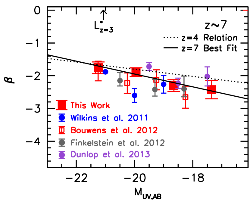
Figure 9.— Comparison of the mean $\beta$’s we find in various $UV$ luminosity ($M_{UV}$) intervals (solid red squares) with those from Wilkins et al. (2011: green circles), Bouwens et al. (2012: open red squares), and Finkelstein et al. (2012: gray circles). The solid black line indicates the best-fit linear relationship between $\beta$ and $UV$ luminosity ($M_{UV}$) for $z\sim 7$ galaxies, while the dotted line shows the relationship we derived for $z\sim 4$ star-forming galaxies (§3.2). Even with the systematic biases now known to exist in previous work (§5 and Appendix B), broad agreement is observed between the present $\beta$ determinations and earlier determinations in the literature.

5. Comparison with Previous Results

5.1. $z\sim 7$ Results: Basic Comparisons

In §4, we have made use of the ultra-deep XDF, HUDF09-Ps, ERS, CANDELS-North, and CANDELS-South observations to obtain the best available constraints on the value of the $UV$-continuum slope $\beta$ for galaxies at $z\sim 7$. The biweight mean $\beta$ we find for sources in our faintest $z\sim 7$ luminosity subsamples is $-2.30\pm 0.18\pm 0.13$. For our brightest $z\sim 7$ subsamples, we find a mean $\beta$ of $-1.75\pm 0.18\pm 0.13$.

Given the comprehensive nature of our analysis, large sample sizes, and essentially bias-free methodology, we would expect our results to be an excellent baseline for evaluating the many different determinations from the literature (Bouwens et al. 2012; Wilkins et al. 2011; Finkelstein et al. 2012; Dunlop et al. 2013). A comparison of the present results with other results in the literature is provided in Figure 9.

5.2. $z\sim 7$ Results: Ascertaining the Nature of the Tension between $\beta$ Results in the Literature

Small, but rather clear differences have existed between the $\beta$ results in the literature, particularly for the lowest luminosity galaxies at $z\sim 7$. This has made for quite a colorful debate, with various groups arguing strongly that the results of other groups may be subject to one or more biases (e.g., Dunlop et al. 2012; Bouwens et al. 2012; Finkelstein et al. 2012; Rogers et al. 2013).

In order to understand the nature of the differences between the many $\beta$ determinations, we have conducted a comprehensive set of comparisons with the large number of $\beta$ measurements already presented in the literature for specific $z\sim 7$ sources (Bouwens et al. 2010, 2012; Finkelstein et al. 2012; Dunlop et al. 2013). These comparisons are presented in great detail in Appendix B and in Figures 18-22 and are performed on an object-by-object basis. While the focus of these comparisons has been on the $\beta$ measurements for individual $z\sim 7$ galaxies, detailed comparisons between the $\beta$ measurements for $z\sim 4$, $z\sim 5$, and $z\sim 6$ galaxies have also been performed (based on the results in §3.2) to obtain the best possible perspective on the types of differences and systematic errors that can occur.

It is not particularly surprising given the debate in the literature on $z\sim 7$ $\beta$ results to observe modest differences in the measured $\beta$’s values for individual $z\sim 7$ sources. In general, the Dunlop et al. (2013) $\beta$ measurements are redder than those found in Finkelstein et al. (2012) which are redder in general than those found in Bouwens et al. (2012). Some differences between the measured $\beta$’s are also evident in the $z\sim 4$-6 results, but in general the differences are smaller.

What is striking in the comparisons (Figures 18-22) is that the observed offsets between the derived $\beta$’s are more dependent on the study making the measurement than on the luminosity or the S/N of the sources where the measurements are made. What this suggests is that the primary explanation for the tension that has existed between $\beta$ results in the literature are systematics in the measurements of the $J_{125}-H_{160}$ colors for individual sources. Given the relatively short lever arm in wavelength one has to establish $\beta$ from the $J_{125}$ and $H_{160}$ photometry, even $\sim$0.04 mag systematics in the measured $J_{125}-H_{160}$ colors are sufficient to explain the discrepancies between the different results in the literature, since such a systematic bias would translate into changes of $\sim 0.18$ in $\beta$.

This is illustrated in Figure 10 for three different measurements of $\beta$ at $z\sim 7$. In this example, while each of these measured $\beta$’s relies on a similar $J_{125}$-band flux measurement, slight differences in the $H_{160}$-band flux measurements are observed. For the sake of illustration, the $H_{160}$-band flux is increased and decreased by small amounts and an assessment of the impact on $\beta$ is made. While the first and third set of flux measurements only show very minor differences relative to the second set of flux measurements, the measured $\beta$’s for the first and third studies differ by $\Delta\beta\sim 0.35$, due to small ($\sim$3-5%) systematics in the measured colors.

If the systematic errors in the measured colors from competing studies are in different directions, we can reconcile all previous $\beta$ measurements for faint galaxies at $z\sim 7$. In particular and as we will show in §5.3-§5.4, we find that the $\beta$ measurements from Bouwens et al. (2012), and likely those from Bouwens et al. (2010), were too blue by $\Delta\beta\sim 0.22$ (see Appendix B.2-B.3) while those from Dunlop et al. (2013) are too red by $\Delta\beta\sim 0.11$-0.18. The Dunlop et al. (2013) bias depends on the size or luminosity of the source (see Figure 11, Appendix B.4, and Figure 25 from Appendix E). See also discussion in Table 6.

5.3. Systematic Biases due to Errors in the PSF

The extensive testing we describe in Appendix B provides strong evidence that systematics in the measured colors can successfully explain the moderately discrepant $\beta$ results obtained in the literature for faint ($-19\lesssim M_{UV,AB}\lesssim-18$) $z\sim 7$ candidates. Of particular relevance for the discussion are the bluer measurements of $\beta$ provided by Bouwens et al. (2012), i.e., $\beta=-2.68\pm 0.19\pm 0.28$ for lower-luminosity ($-18.75<M_{UV,AB}<-17.75$) $z\sim 7$ galaxies.

The tests in Appendix B.3 clearly indicate a $\sim 0.05$ mag bias in the measured $J_{125}-H_{160}$ colors from Bouwens et al. (2012). The source of this systematic error appears to occur as a result of the PSF-matching that Bouwens et al. (2012) perform. To investigate this issue in detail, we conducted detailed comparisons between the encircled energy distributions implied by the Bouwens et al. (2012) empirically-derived PSFs and standard determinations of these encircled-energy distributions (Dressel et al. 2012). We found that the $J_{125}$-band PSF from Bouwens et al. (2012) showed slightly more energy ($\sim$3%) at intermediate radii, i.e., $\sim 0.15$-$0.20$^′′, relative to the Dressel et al. (2012) encircled-energy distributions in the $J_{125}$ band. The wings of the empirically-derived $J_{125}$-band PSF also contained 2% less flux than in the wings of the $H_{160}$-band PSF (relative to what should have been the case given the Dressel et al. 2012 encircled-energy distributions). Together these effects would cause the measured $J_{125}$-band fluxes from Bouwens et al. (2012) to be systematically bright by $\sim$0.05 mag. This would result in $\beta$ determinations from Bouwens et al. (2012) that are too blue by $\Delta\beta\sim$0.22.

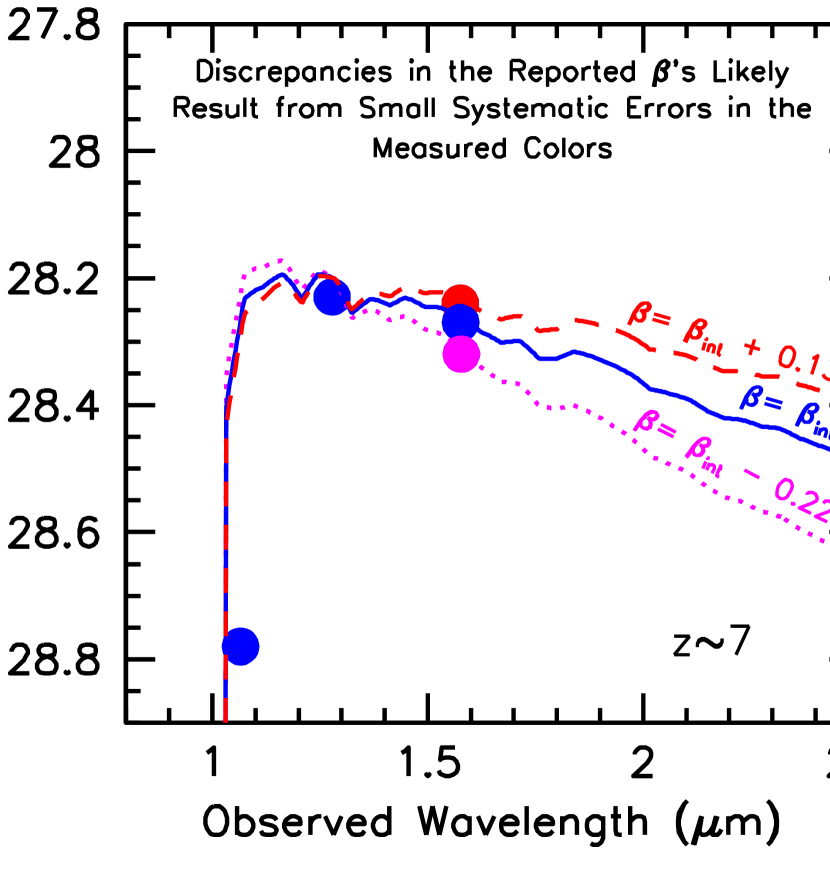
Figure 10.— Illustration of how small $\sim$0.03-0.05-mag systematic errors in the measured $J_{125}-H_{160}$ colors for $z\sim 7$ galaxies can result in large differences in the measured $\beta$’s (§5.2-5.4). Each of the measured $\beta$’s shown in this figure relies on a similar $J_{125}$-band flux measurement, but with slight differences in the $H_{160}$-band flux measurements in three “studies.” Compared to the first study, the second study measures a $H_{160}$-band flux 0.03 mag fainter than the first study, while the third study measures a $H_{160}$-band flux 0.08 mag fainter than the first. Both the first and third set of flux measurements only show very minor differences relative to the second set of flux measurements, yet the measured $\beta$’s for the first and third studies differ by $\Delta\beta\sim 0.35$, due to small ($\sim$3-5%) systematics in the measured colors. The change in $\beta$ from very small differences in colors is dramatic. Changes this large, especially if the systematic errors in the measured colors from competing studies are in different directions, can actually reconcile all previous $\beta$ measurements for faint galaxies at $z\sim 7$ (see the text in §5.2).

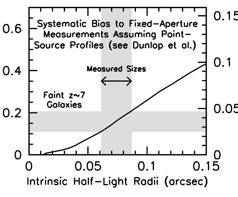
Figure 11.— Systematic bias in the estimated $UV$-continuum slopes $\beta$ (and $J_{125}-H_{160}$ color) of $z\sim 7$ galaxies one would expect as a function of the intrinsic half-light radii of sources, if one treats all $z\sim 7$ candidates as point sources and performs photometry in fixed filter-dependent apertures enclosing 70% of the light for a point source (e.g., Dunlop et al. 2013). For sources with $UV$ luminosities in the $-19.3\lesssim M_{UV,AB}\lesssim-18$ range, half-light radii estimates have ranged from 0.06^′′ to 0.09^′′ (Oesch et al. 2010; Ono et al. 2013). We find a half-light radius of 0.074$\pm$0.013^′′, by using galfit to fit a stack of the sources in this magnitude range. Based on these size estimates, we find that the above photometric procedure would result in a systematic bias of $\sim$0.03 to $\sim$0.04 mag to the red in the $J_{125}-H_{160}$ color and a bias of $\sim$0.11-0.18 in $\beta$ (see also Figure 25). Correcting the Dunlop et al. (2013) measurements for this bias, we can fully reconcile discrepancies between their measurements and our own (see §5.4, Appendix B.4.4, and Figure 16).

5.4. Biases Caused by Applying Point-Source Aperture Photometry to Sources with Non-Zero Size

The tests that we describe in Appendix B.4 also revealed small systematic biases in the photometry of Dunlop et al. (2013), particularly for the most luminous sources. We found that the magnitude of the bias was a function of source size. Source size does not have an impact on the accuracy of color measurements when performing photometry in identical apertures, after PSF-matching the observations, as was done by Bouwens et al. (2012) and Finkelstein et al. (2012). However, Dunlop et al. (2013) utilize a different approach for performing photometry, measuring the flux in fixed filter-dependent circular apertures that enclose 70% of the light for a point source. Dunlop et al. (2013) find that the 70% encloded flux occurred in 0.44^′′-diameter, 0.47^′′-diameter, and 0.50^′′-diameter circular apertures for the $J_{125}$, $JH_{140}$, and $H_{160}$ band observations, respectively. While this approach would provide accurate colors if faint $z\sim 7$ galaxies were point sources, small systematics will be present in the $J_{125}-H_{160}$ color measurements since $z\sim 7$ galaxies are spatially extended. The effect of assuming point sources instead of using the actual profiles leads to a surprisingly significant bias.

This bias occurs because non-zero sizes of sources result in a larger percentage of the light being pushed to larger radii, relative to the expectations for a point source. We can estimate the size of this bias by stacking galaxies from our own $z\sim 7$ samples and then deriving the encircled energy distribution. For stacks of the galaxies from different luminosity subsamples in our XDF data set, we found 11-14% more flux in 0.50^′′-diameter apertures than in 0.44^′′-diameter apertures, with the largest excesses being present for the most extended sources. This compares with just $\sim$8% more light in the larger aperture for stars. We found essentially identical results in all WFC3/IR bands, indicating a likely 3-6% systematic error in the $J_{125}-H_{160}$ colors performing the color measurement in this way. While small, this is sufficient to have a noticeable effect on $\beta$. We repeated these tests on the Koekemoer et al. (2013) HUDF12 reductions and found essentially identical results.

An alternative approach to deriving the color bias is by fitting the $z\sim 7$ stack to a model profile, measuring the half-light radii, and then computing the bias one would expect from that half-light radius. Let us focus on sources with UV luminosities in the $-19.3\lesssim M_{UV,AB}\lesssim-18$ range. Using galfit (Peng et al. 2002) to fit the stacked profile (assuming an exponential profile), we find a half-light radius of $0.074\pm 0.013^{\prime\prime}$. Both the mean half-light radius and error on this measurement were made by repeating this measurement in all four WFC3/IR bands and computing the mean and variance (the smallest size measurement was in the $Y_{105}$ band). Oesch et al. (2010) and Ono et al. (2013) find similar half-light radii, i.e., 0.06^′′ to 0.09^′′.

We computed the implied encircled energy distribution for a galaxy with this scale length by first creating a model profile with the same scale length, convolving it with the $J_{125}$ and $H_{160}$ band PSFs, and then computing the fraction of the total flux inside a $0.44^{\prime\prime}$-diameter aperture in the $J_{125}$ band and $0.50^{\prime\prime}$-diameter aperture in the $H_{160}$ band. Then, by comparing these fractions to the expected fraction (i.e., 70%) for a point source, we estimated the likely bias in the Dunlop et al. (2013) $J_{125}-H_{160}$ color measurements. Using this procedure, we concluded that there would be a 0.03 mag redward bias in the $J_{125}-H_{160}$ colors for $M_{UV,AB}\sim-18.6$ galaxies. This would be equivalent to a $\Delta\beta$ $\sim$0.13 bias in $\beta$. The expected biases for $z\sim 7$ galaxies with other half-light radii are presented in Figure 11. We would expect the most substantial biases to occur for the brightest (and typically largest) sources. The comparisons presented in Appendix B.4 and Figure 22 also show the trends expected based on these tests (and similarly for the simulations presented in Figure 25 from Appendix E).

5.5. Reconciling $\beta$ Results for Faint Sources at $z\sim 7$

In §5.3-5.4, we identified small systematic biases in the measured $\beta$’s derived by Bouwens et al. (2012) and Dunlop et al. (2013). These biases would cause the measured $\beta$’s from Bouwens et al. (2012) to be $\Delta\beta\sim 0.22$ too blue and the measured $\beta$’s of Dunlop et al. (2013) to be $\Delta\beta\sim 0.13$ too red. The comparisons we performed in Appendix B.1 show no statistically-significant offset between our current results and those of Finkelstein et al. (2012), though there are concerns that the Finkelstein et al. (2012) $\beta$ determinations could be affected by the use of broadband fluxes affected by Ly$\alpha$ emission (e.g., see Figure 12 from Rogers et al. 2013).

Correcting the $\beta$ results of the Bouwens et al. (2012) and Dunlop et al. (2013) for the biases identified above, we can approximately reconcile all the results in the literature on $\beta$ for faint $z\sim 7$ galaxies. Our suggested revisions to published measurements are presented in Table 6 for galaxies in the luminosity range $-19\lesssim M_{UV,AB}\lesssim-18$ which has been the focus of recent debate. The corrected results extend over the range $\beta\sim-2.5$ to $\beta\sim-2.3$. One can see that the results are all consistent with each other within the $1\sigma$ statistical errors of each study.

It is worthwhile noting that this range in $\beta$, i.e., $-2.3$ to $-2.5$, also includes the $\beta=-2.5\pm 0.06$ measurement recently obtained for one highly-magnified, lower-luminosity $z\sim 6.2$ galaxy found in the CLASH program. The existence of this source clearly demonstrates that some lower-luminosity galaxies in the redshift range $z\sim 6$-8 do have $\beta$’s as blue as $-2.5$. Also found within this range is the median $\beta=-2.3$ measurement from Jiang et al. (2013) for their sample of $z\sim 6.6$ LAEs (although the intrinsic luminosities of the Jiang et al. 2013 LAE sample are clearly larger, one would expect a Ly$\alpha$-emitting population to be bluer on average than the typical luminous galaxy: Stark et al. 2010).

Based on these comparisons, we can also understand why the mean $\beta$ for faint sources measured in Bouwens et al. (2010) differ from those given here or from others in the literature. The shift from a $\beta$ of $\sim-3.0$ to the $\sim-2.4$ (the mean $\beta$ we measure for $z\sim 7$ galaxies from the HUDF using the same binning scheme) resulted from three effects: (1) a $\sim$0.05 mag systematic error in the measured $J_{125}-H_{160}$ color to the blue (resulting in a $\Delta\beta\sim 0.2$ systematic bias), (2) a $\Delta\beta\sim 0.1$ noise-driven systematic bias (see Appendix B.2), and (3) statistical noise in the measurements due to the limited depth of the early WFC3/IR observational data.

5.6. Other Considerations In Comparing $\beta$ Results

In addition to the detailed issues just discussed, other effects can be important in comparing the central values for $\beta$. For example, whether one uses a mean or median to define the center of the $\beta$ distribution needs to be considered, given that the mean values for $\beta$ are typically $\Delta\beta\sim 0.1$ redder than the median values, due to the tail in the $\beta$ distribution to redder values (e.g., compare the biweight means, medians, and inverse-variance-weighted means reported in Table 2). The biweight mean is our preferred measure.

Finally, the value of $\beta$ one derives can also show some dependence ($\Delta\beta\sim 0.2$) on the precise filter set or wavelength range one uses to estimate $\beta$. This is due to the fact that the $UV$ continuum in star-forming galaxies is almost certainly not a precise power law. The inset to Figure 27 provides a direct illustration on how significant such effects can be (and how these effects even depend on the precise star formation history one assumes for individual galaxies). See also Figure 2 from Rogers et al. (2013) who noted that $\Delta\beta$ differences as large as 0.2 in the measured values for $\beta$ depending on how one made the measurement.

The point here is that $\beta$ results, particularly at the highest redshifts where the available leverage in wavelength is small, can be extraordinarily sensitive to small systematics in the photometry and model dependencies in one’s analysis technique.

5.7. Summary

In summary, by conducting a comprehensive set of comparisons with the source-by-source $\beta$ measurements from previous studies, we have succeeded in identifying a number of small but important systematic errors in previous measurements of $\beta$ at $z\sim 7$. We find that the $\beta$ measurements from Bouwens et al. (2012) were too blue by $\Delta\beta\sim 0.22$. The $\beta$ measurements of Dunlop et al. (2013), by contrast, are too red by $\Delta\beta\sim 0.11$-0.18 in the luminosity interval $-19<M_{UV,AB}<-18$. The $\beta$ results of Dunlop et al. (2013) likely show larger biases brightward of $-19$ and smaller biases faintward of $-18$. While no statistically significant systematic errors were identified in the $z\sim 7$ $\beta$ measurements from Finkelstein et al. (2012), their results are nonetheless susceptible to small measurement biases due to their using flux information contaminated by Ly$\alpha$ emission (e.g., see Rogers et al. 2013). After accounting for these systematic errors, we are able to successfully reconcile all previous results for $\beta$ at $z\sim 7$.

6. $\beta$ Results for $z\sim 8$-8.5 Samples

The availability of very deep $JH_{140}$ observations over the HUDF allows for the possibility of establishing the mean value of the $UV$-continuum slope $\beta$ to $z\sim 8$ and even $z\sim 8.5$. These new $\beta$ determinations should provide us with additional leverage for constraining the evolution of the $UV$-continuum slope $\beta$ to early times.

6.1. Methodology for $z\sim 8$ Sample

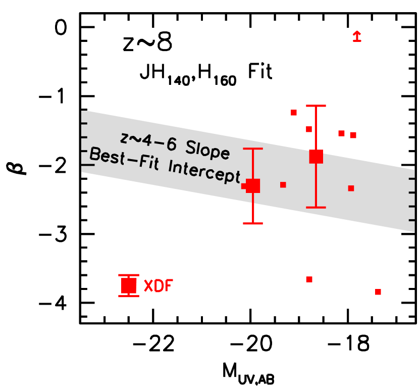
Figure 12.— (left) Measured $\beta$’s versus the rest-frame $UV$ luminosity $M_{UV}$ for galaxies in our $z\sim 8$ sample from the XDF. The $\beta$’s we present here are based on the $JH_{140}-H_{160}$ colors of $z\sim 8$ sources in our samples. Sources which yield a $\beta$ in the range of this figure are shown as the small red squares, while the one source with derived $\beta$’s beyond the vertical bounds of this plot are shown as a lower limit. The large red squares give the weighted-mean $\beta$’s observed in various bins of $UV$ luminosity. Despite the small amount of wavelength leverage available using $JH_{140}$ and $H_{160}$-band photometry, the $JH_{140}-H_{160}$ color allows for a clean measurement of $\beta$ in $z\sim 8$ sources. It is not possible to obtain an entirely clean measurement of $\beta$ for $z>8$ galaxies, if one includes the $J_{125}$-band flux in estimating $\beta$ (see Figure 27). The gray-shaded band shows the $1\sigma$ range allowed for a fit to the $\beta$-$M_{UV}$ relation fixing the slope of this relation to the average value ($-0.13$) found by Bouwens et al. (2012) for $z\sim 4$-6 galaxies.

Our $z\sim 8$ selection criteria are as follows:

$$(Y_{105}-J_{125}>0.8)\wedge(J_{125}-H_{160}<0.5)$$

We constructed these criteria to be complementary to those used to select sources in our $z\sim 7$ sample, so these criteria are useful in selecting galaxies with redshifts just higher than those selected by our $z\sim 7$ criteria. Sources must also by necessity be undetected at $<2\sigma$ in each optical/ACS band. Finally, we require the computed $\chi^{2}$ statistic for the sources (computed from their $B_{435}V_{606}i_{775}I_{814}z_{850}$ fluxes) not be greater than 3 in any of the three apertures we use ($0.18^{\prime\prime}$-diameter aperture, scaled aperture, $0.35^{\prime\prime}$-diameter aperture).

Our primary method for deriving $UV$-continuum slopes for $z\sim 8$ galaxies is based on a power-law fit to the $JH_{140}$ and $H_{160}$ band fluxes. Given that we have only two constraints on the power law slope using fluxes in these bands, this approach is functionally equivalent to using a fitting formula

$$\beta=-2.0+8.98(JH_{140}-H_{160}).$$ (2)

The coefficients in this fitting formula are derived assuming galaxies have a $\beta=-2$ spectrum. Given that Ly$\alpha$ emission or the Lyman break only begin to enter the $JH_{140}$ band at $z\gtrsim 9$, the $JH_{140}-H_{160}$ color should allow for a totally clean measurement of the spectral slope $\beta$ in $z\sim 8$ sources.

The challenge with this approach is the very small effective wavelength difference between the $JH_{140}$ and $H_{160}$ filters. This makes the derived $\beta$’s extremely sensitive to any uncertainties or systematics in the measured $JH_{140}-H_{160}$ colors. Minimizing the systematics is therefore essential. For this reason, care was taken not only in PSF-matching the observations (Appendix A), but in testing the accuracy of the $JH_{140}-H_{160}$ color measurements. The most relevant test here was comparing the $UV$-continuum slopes $\beta$ we derived based on the $JH_{140}-H_{160}$ colors for $z\sim 7$ galaxies with $UV$-continuum slopes $\beta$ derived based on the $J_{125}$, $JH_{140}$, and $H_{160}$ photometry. A median difference of $\Delta\beta\sim 0.05$ was found between the two sets of $\beta$’s, with sources with the $JH_{140}$+$H_{160}$-derived $\beta$’s being slightly redder overall. Since such differences are well within the expected statistical uncertainties, this test strongly suggested that our $JH_{140}-H_{160}$ colors did not suffer from large systematic biases.

One alternate approach for deriving the $UV$-continuum slopes $\beta$ at $z\sim 8$ involves leveraging the available $J_{125}$, $H_{160}$, and $JH_{140}$ (where available) photometry for sources. Such an approach has previously been utilized by Dunlop et al. (2013). The primary advantage of using such an approach is the much greater leverage in wavelength one has taking advantage of the $J_{125}$-band photometry. $J_{125}$-band observations are also more widely available over legacy fields (e.g., CANDELS and HUDF09-2) than are $JH_{140}$-band observations. This approach, unfortunately, suffers from one major systematic drawback. The measured $\beta$’s can be subject to large redward biases, e.g., $\Delta\beta\sim 1$, if the galaxies one is examining have redshifts in excess of $z\gtrsim 8$. The large biases result from the effect of the IGM on the $J_{125}$-band flux. Figure 27 from Appendix G illustrates how large such biases can be. While these large biases may seem straightforward to avoid, uncertainties in the photometric redshifts of individual sources make it challenging to determine the precise correction that should be applied to the $J_{125}$-band fluxes of individual sources.

Because of these biases and the significant assumptions required to correct for them, no use of the $J_{125}$-band fluxes is made in quantifying $\beta$ for our baseline $z\sim 8$ study. For completeness, however, we consider such an approach in Appendix G.

6.2. $\beta$ Results for $z\sim 8$ Sample

The $\beta$ measurements we obtain for individual galaxies in our $z\sim 8$ samples are presented in Figure 12. Also shown are the biweight mean $\beta$’s for the $z\sim 8$ galaxies in specific bins in $UV$ luminosity. The results for the median $\beta$’s are similar, albeit slightly redder in the $M_{UV}=-18.5$ bin. We determine the linear relationship which best fits the mean $\beta$’s we find at a given $M_{UV}$ luminosity. Due to the large uncertainties on the binned $\beta$ determinations, no attempt is made to determine the slope of the $\beta$ vs. $M_{UV}$ relationship at $z\sim 8$. We simply assume that the slope of this relationship at $z\sim 8$ is the same as the average slope we find for this relationship at $z\sim 4$-6, i.e., $-0.15$ (e.g., Table 3). The binned $\beta$’s and coefficients to the best-fit $\beta$ vs. $M_{UV}$ relationship are presented in Table 2 and 3.

The inverse-variance-weighted mean $\beta$ we measure for lower-luminosity ($\sim-18$ mag) $z\sim 8$ galaxies is $-$1.88$\pm$0.74$\pm$0.27 using only the $JH_{140}$+$H_{160}$-band flux information. In Appendix G, using the flux information in the $J_{125}$+$JH_{140}$+$H_{160}$ bands (after correcting for the impact of the IGM), we find $-2.39\pm 0.35\pm 0.13$ for faint $z\sim 8$ galaxies in this same magnitude interval. The current measurements are consistent with the $\beta=-2.03_{-0.38}^{+0.46}$ and $\beta=-1.88_{-0.56}^{+1.03}$ measurements obtained by Finkelstein et al. (2012) for $z\sim 8$ galaxies found over a similar range of luminosities, though the errors are so large in both data sets that consistency does not indicate robust agreement. The $\beta=-1.9\pm 0.3$ measurements from Dunlop et al. (2013) are also consistent with the $\beta$’s we derived here. However, for the Dunlop et al. (2013) study, a slight revision to the $z\sim 8$ $\beta$ results is required to correct for the slight bias in $\beta$ due to non-zero sizes of $z\sim 8$ sources (e.g., see Figure 11, §5.4, and Appendix B.4) and to correct for the effect of the IGM on the $J_{125}$-band fluxes of $z\sim 8$ galaxies in their samples (see Figure 27 and Appendix G). Correcting for both effects results in a revision of their mean $\beta$ measurement at $z\sim 8$ to $\beta\sim-2.1\pm 0.3$.

Regardless of the approach and dataset the current $z\sim 8$ derivations of $\beta$ are all highly uncertain and do not add particularly strong constraints because of the small sample sizes, sensitivity to photometric uncertainties because of the limited filter separation, and systematic biases. The most useful constraints in the reionization epoch are still to be found at $z\sim 7$.

6.3. $\beta$ Results for a Small $z\sim 8.5$ Sample

Finally, it is possible to try to take advantage of the small number of $z\sim 8.5$-9 candidates that have recently been identified in the literature (Zheng et al. 2012; Bouwens et al. 2013; Ellis et al. 2013; Oesch et al. 2013b) to see what constraints can be set on $\beta$ for galaxies in this redshift range.

Measuring $\beta$ for galaxies at $z\sim 8.5$ and higher is extremely challenging at present. There are a number of reasons for this: (1) the small number and extreme faintness of most $z\sim 9$ candidates, (2) the short lever arm in wavelength to constrain $\beta$, and (3) the rather significant effect the IGM would have on the observed fluxes in the $JH_{140}$-band, if any of the candidates had redshifts in excess of $z\sim 9$. This final effect is particularly important, since even a 10% lower flux in the $JH_{140}$-band due to absorption from the IGM (expected for sources at $z\sim 9.3$) would bias the measured $\beta$’s by the large factor $\Delta\beta\sim 0.9$. To successfully correct for this bias would require accurate constraints on the redshifts for individual sources. Unfortunately, almost every $z\sim 9$ candidate known has redshift uncertainties of $\sigma(z)\gtrsim 0.7$, so even corrections for the average source would not be particularly effective at eliminating this bias.

Due to the very large random and potential systematic uncertainties in estimates of $\beta$ at $z\sim 9$, it is perhaps best if we only consider those $z\sim 8.5$ candidates which are the brightest and photometrically well-constrained. Given that the majority of the $z\sim 9$ candidates in the Oesch et al. (2013b) and Ellis et al. (2013) samples have a S/N of $\sim$3-4 in individual bands, this leaves us with just two $z\sim 9$ galaxy candidates that we can examine where our $\beta$ measurements would be likely clean, i.e., XDFyj-38135540 and XDFyj-39478076 from Oesch et al. (2013b). Unfortunately, all three lensed candidate $z\sim 9$ galaxies from the CLASH program (Postman et al. 2012), i.e., MACS1149-JD ($z\sim 9.7$), MACSJ1115-JD1 ($z\sim 9.2$), and MACSJ1720-JD1 ($z\sim 9.0$: Zheng et al. 2012; Bouwens et al. 2013) do not qualify since their estimated redshifts are quite likely in excess of $z\sim 9$ (particularly MACS1149-JD), and therefore even their $JH_{140}$-band fluxes are substantially affected by IGM absorption.

For these two sources, we estimate $\beta$ using the $JH_{140}-H_{160}$ color using the same formula $\beta=8.98(JH_{140}-H_{160})-2$ we presented in §6.2 for $z\sim 8$ sources in our samples. Based on these two $z\sim 8.5$ sources, we derive an inverse-variance-weighted mean $\beta$ of $\sim-2.1\pm 0.9$. The mean $\beta$ is $-1.8$. Given the large uncertainties, this determination is consistent with our $z\sim 7$ and $z\sim 8$ determinations.

Previously, Dunlop et al. (2013) have presented an approximate measurement of the mean $\beta$ for galaxies at $z\sim 9$ based on a small number of sources from the XDF. While the present measurement is, of course, consistent with the Dunlop et al. (2013) estimate, the present estimate of the mean $\beta$ at $z\sim 8.5$ is more reliable, though it is not particularly meaningful given the uncertainties. First of all, Dunlop et al. (2013) have included a large number of galaxies with photometric redshifts consistent with being at $z\sim 9$. Including these sources is dangerous, since as we emphasized earlier any candidate with a redshift in excess of $z\sim 9$ would be strongly biased (e.g., $\Delta\beta\gtrsim 1$) to redder $\beta$ values (see e.g. Figure 27). It is therefore concerning that the $z\sim 9$ sample of Dunlop et al. (2013) includes one and possibly two $z\sim 9$ candidates generally agreed to be at $z>9$ (Ellis et al. 2013; Oesch et al. 2013b). This will result in a clear redward bias.

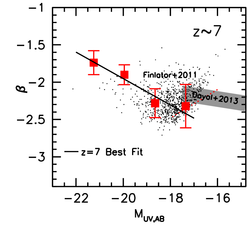
Figure 13.— A comparison of the mean $UV$-continuum slopes $\beta$ vs. $UV$ luminosity relationship found here for our $z\sim 7$ sample (red solid squares) with that predicted in the Finlator et al. (2011) hydrodynamical simulations (black points). The dotted red line shows where incompleteness becomes important for the results from the simulations. The mean $\beta$ expected in the $UV$ luminosity range $-19<M_{UV,AB}<-18$ by the simulations is $\sim-2.3$. Also shown on this plot are the predicted trends at $M_{UV}>-18$ from the simulations of Dayal et al. (2013: gray shaded region).

Second, as Oesch et al. (2013b) have demonstrated, the $z\sim 9$ sample used by Dunlop et al. (2013: see also Ellis et al. 2013) includes a source HUDF12-4106-7304 whose flux is substantially boosted (i.e., factor of $\sim$2) by a diffraction spike from a bright nearby galaxy (Figure 9 from Oesch et al. 2013b). Not only does this cast considerable doubt on the reality of this source (now only $2.8\sigma$ significance), but it would bias its photometry as well.

For the above reasons, we consider the current measurement of the mean $\beta$ at $z\sim 8.5$ to be the highest redshift, reliable estimate of $\beta$ at present (although given the large uncertainties on this measurement it is not really meaningful at present).

7. Discussion and Physical Implications

In this present analysis, we have made use of the extremely deep WFC3/IR observations over the XDF, HUDF09-Ps, CANDELS-North, CANDELS-South, and ERS fields to establish the distribution of $UV$-continuum slopes $\beta$ for $z\sim 4$-8 galaxies while ensuring that the systematic errors are minimized.

As in our previous study, we found strong evidence for a correlation between $\beta$ and $UV$ luminosity for star-forming galaxies at $z\sim 4$, $z\sim 5$, $z\sim 6$, and $z\sim 7$, with higher luminosity galaxies being redder and lower luminosity galaxies being bluer at all redshifts. The existence of such a relationship is likely largely driven by changes in the mean metallicity or dust extinction of galaxies as galaxies grow in stellar mass and $UV$ luminosity (Bouwens et al. 2009; Bouwens et al. 2012; Finkelstein et al. 2012). The slope of the $\beta$ vs. $UV$ luminosity relationship appears to be roughly constant as a function of redshift or cosmic time (e.g., see Figure 2).

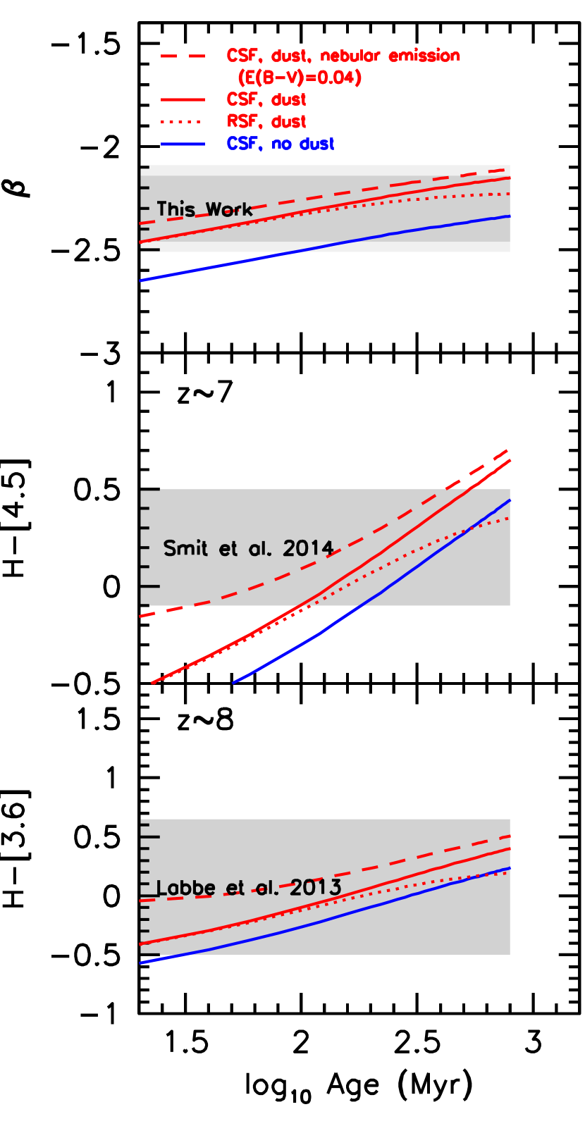
Figure 14.— (upper) Predicted $UV$-continuum slope $\beta$ for a constant star formation model versus age. Shown are the predictions assuming no dust extinction (blue line) and for a $E(B-V)=0.04$ model (red line). Model tracks are shown from zero age to the age of the universe at $z\sim 7$. 0.5 $Z_{\odot}$ metallicity is assumed, similar but slightly higher than the predictions for faint galaxies at high redshift (Finlator et al. 2011; Dayal & Ferrara 2011; Wise et al. 2012). The dark shaded gray region shows the 68% confidence interval on the mean value for $\beta$ observed in faint ($-19.3\lesssim M_{UV,AB}\lesssim-18.0$) $z\sim 7$ galaxies. Also shown are the predictions for an exponentially-increasing star formation history (red dotted line) with $\tau=5\times 10^{8}$ years and including nebular-continuum emission (red dashed line: see Oesch et al. 2013a). (middle) Predicted $H_{160}-[4.5]$ colors for the same constant star formation models as shown in the upper panel. The 68% confidence interval on the average $H_{160}-[4.5]$ color of $z\sim 7$, $M_{UV}\sim-20$ galaxies from the CLASH program (Smit et al. 2014) is indicated by the shaded region. (lower) Predicted $H_{160}-[3.6]$ colors for the same constant star formation models as shown in the upper panel. The 68% confidence interval on the average $H_{160}-[3.6]$ color of $z\sim 8$, $M_{UV}\sim-19$ galaxies from the HUDF09 fields (Labbé et al. 2013) is indicated by the shaded region. The mean $\beta$’s and $H_{160}-IRAC$ colors we derive here for lower luminosity $z\sim 7$ galaxies are broadly consistent with stellar population ages from 50 Myr to 600-800 Myr (age of the universe at $z=7$-8) and dust extinction from $E(B-V)=0.0$ to $E(B-V)\sim 0.06$.

The primary focus of this study was to establish reliable and bias-free measures of $\beta$ for $z\sim 7$ galaxies at very low luminosities. To support this goal, we also leveraged the deepest-ever optical+near-IR HST observations to establish the mean $UV$ slope $\beta$ for faint galaxies in four other redshift intervals $z\sim 4$, $z\sim 5$, $z\sim 6$, and $z\sim 8$ to determine the trend with redshift. Mean $\beta$’s of $-2.03\pm 0.03\pm 0.06$, $-2.14\pm 0.06\pm 0.06$, $-2.24\pm 0.11\pm 0.08$, and $-2.30\pm 0.18\pm 0.13$ are found for faint galaxy selections at $z\sim 4$, $z\sim 5$, $z\sim 6$, and $z\sim 7$ galaxies, respectively. The mean $UV$ slopes of the faint galaxies at $z\sim 8$ and $z\sim 8.5$ are consistent with the values found above, but are too uncertain to play a role in any discussion of the trends.

Similar to the previous results presented in Bouwens et al. (2012), these results are consistent with the mean $UV$-continuum slope $\beta$ of galaxies only evolving gradually as a function of cosmic time, if one examines galaxies at the same $UV$ luminosity or stellar mass at all epochs. Figure 4 provides a good illustration of the observed trends.

The $UV$ slopes of the faint galaxies we find in $z\sim 8$ and $z\sim 8.5$ selections are consistent with the blue values found above, but are nonetheless quite uncertain. Consistent with these trends, the faintest galaxies at $z\sim 7$ show evidence for exhibiting somewhat bluer $\beta$’s, i.e., $\beta\sim-2.3$-2.4 at $z\sim 7$-8. This is evident for our results from the XDF and HUDF09-Ps fields and for our $-19.3<M_{UV,AB}<-18.0$ and $-18.0<M_{UV,AB}<-16.7$ subsamples from those fields.

At lower luminosities, our mean $\beta$ results at $z\sim 7$ are in excellent agreement with the results from cosmological hydrodynamical simulations, such as those performed in Finlator et al. (2011), as shown in Figure 13. The agreement is less easy to discern in the faintest luminosity bin, due to incompleteness in the simulation results at low masses. However, in the luminosity bin $-19.3<M_{UV,AB}<-18.0$, the mean $\beta$ from the simulations is $\sim-$2.33, consistent with the mean $\beta$ we report $-2.30\pm 0.18\pm 0.13$. Also shown on this diagram are the results from Dayal et al. (2013) for very faint $M_{UV,AB}>-18$ galaxies at $z\sim 7$ and again the agreement is excellent.

What do the present results imply for the stellar populations of faint $z\sim 7$-8 galaxies? In Figure 14, we include a figure showing the predicted $UV$-continuum slope $\beta$ for galaxies as a function of the stellar population age assuming a constant rate of star formation. The results are shown for both the case with no dust extinction ($E(B-V)=0.0$) and a small amount of dust extinction ($E(B-V)=0.04$). Dust extinction is implemented using the Calzetti et al. (2000) prescription. The metallicity of galaxies is assumed to be 0.5 $Z_{\odot}$, which is similar but slightly higher than the expectations of simulations (Davé et al. 2006; Finlator et al. 2011).

Comparing the mean $\beta$’s we derive for the faintest galaxies at $z\sim 7$ with the model predictions, the observed $\beta$’s are suggestive of a dust extinction that is not substantially higher than $E(B-V)=0.06$. No significant constraints can be set on the mean age of the stellar population. On the basis of a redder derived $\beta$, Dunlop et al. (2013) favored a model with slightly higher dust extinction than what we prefer here (equivalent to $E(B-V)\sim 0.05$).

We can also potentially gain insight into the stellar populations of $z\sim 7$-8 galaxies by comparing against the observed rest-frame $UV$ to optical colors of $z\sim 7$ and $z\sim 8$ galaxies. This requires we make use of flux measurements with IRAC to constrain the rest-frame optical fluxes. This is somewhat challenging due to the strong emission lines in these sources that contaminate the observed IRAC fluxes (e.g., Schaerer & de Barros 2009; de Barros & Schaerer 2014; González et al. 2012, 2014; Stark et al. 2013; Labbé et al. 2013). Fortunately, there are specific redshift windows where one can obtain relatively clean measurements of the rest-frame optical flux (e.g., Stark et al. 2013). Smit et al. (2014) exploited one such redshift window $z\sim 6.6$-7.0 to obtain a constraint on the $H_{160}-[4.5]$ color for moderately faint ($\sim-20.0$ mag) $z\sim 7$ galaxies (albeit slightly brighter than we consider here). Meanwhile, Labbé et al. (2013) exploited another such redshift window $z\gtrsim 7.1$ to obtain a relatively clean constraint on the $H_{160}-[3.6]$ color for faint $H_{160,AB}\sim 28$ galaxies.

The observational constraints are shown in the middle and lowest panels of Figure 14 and can be compared with the results from stellar population models. No strong constraints on the age of the stellar population can be set. Ages from $\sim$50 Myr to 800 Myr (age of the universe) are formally allowed, though the real upper limit is set by the onset of the earliest significant star formation in the universe (which is currently thought to occur at ages around 150-200 Myr after the Big Bang). For stellar population ages of $\sim$200 Myr, the joint constraints on $\beta$ and $UV$-to-optical colors suggest a non-zero dust extinction in these sources, with a best-fit value of $E(B-V)\sim 0.02$. Unfortunately, the available IRAC observations are simply not deep enough at present to set strong constraints on UV-to-optical colors of $z\sim 7$-8 galaxies and hence their stellar population models. Dunlop et al. (2013) also drew somewhat similar conclusions to these, despite modest differences in their preferred values for $\beta$ (see also the simulation results from Wilkins et al. 2013).

As in our previous study (e.g., Bouwens et al. 2012), the present results provide no significant evidence for exotic or unusual stellar populations, consistent with the results from many recent studies (Finkelstein et al. 2010, 2012; Wilkins et al. 2011; Dunlop et al. 2012).

Table 7Systematic Biases that have likely affected previous studies of $\beta$ at $z\sim 7$.

	Systematic	Magnitude of
	(potential &	Bias
Paper	demonstrated)	($\Delta\beta$)
Bouwens et al. 2010	Photometric Error	$-$0.1
	Coupling Bias
	PSF-Matching Bias	$-$0.22
Finkelstein et al. 2010	Photometric Error	$-$0.5(?)
	Coupling Bias
	Selection Volume Bias	Uncorrected
Wilkins et al. 2011	Photometric Error	Uncorrected
	Coupling Bias
Dunlop et al. 2012	Photometric Error	Uncorrected
	Coupling Bias
	Selection Volume Bias	Uncorrected
Bouwens et al. 2012	PSF-Matching Bias	$-$0.22
Finkelstein et al. 2012	Ly$\alpha$ contamination	Uncorrected
	Bias
	Selection Volume Bias	Uncorrected
Dunlop et al. 2013	Non-Zero Size Bias	$+$0.13
	Selection Volume Bias	Uncorrected

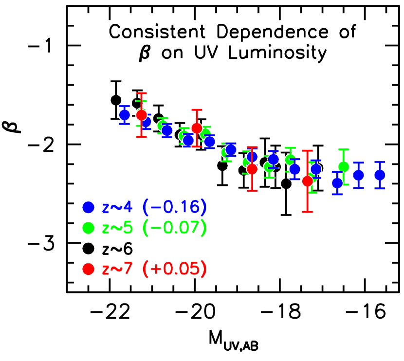
Figure 15.— Biweight mean $UV$ continuum slope $\beta$ derived versus $UV$ luminosity for our $z\sim 4$, $z\sim 5$, $z\sim 6$, and $z\sim 7$ galaxy samples (see §3.2 and §4.7). Slight offsets to the $\beta$ results from our $z\sim 4$, $z\sim 5$, and $z\sim 7$ samples have been applied, i.e., $\Delta\beta\sim-0.16$, $\Delta\beta\sim-0.07$, $\Delta\beta\sim 0.05$, to better illustrate the consistent dependence on luminosity. Only a small amount of evolution in the $\beta$ vs. $M_{UV}$ relationship is observed as a function of redshift. It is clear that $\beta$ shows a consistent dependence on $UV$ luminosity at all redshifts, with a clear trend to bluer colors at lower luminosities. The dependence of $\beta$ on luminosity becomes weaker at the lowest luminosities (see Figure 3 and §3.4).

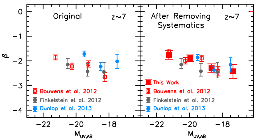
Figure 16.— Mean $\beta$ as a function of $UV$ luminosity, before correction for the systematic biases we identified in this study (left) and after correction (right). The two prominent biases that we have identified in the $z\sim 7$ $\beta$ measurements are a $\Delta\beta\sim 0.22$ blueward bias in the Bouwens et al. (2012) measurements (see Appendix B.3) and $\Delta\beta\sim 0.13$ redward bias in the Dunlop et al. (2013) measurements (§5.4 and Appendix B.4). That Dunlop et al. (2013) suffer from a $\Delta\beta\gtrsim 0.13$ bias in their $\beta$ measurements can be demonstrated using the measured sizes for faint $z\sim 7$ galaxies (see Figure 11) and from detailed object-by-object comparisons with the $\beta$ results from Finkelstein et al. (2012) and the present study (see Figure 22). After correcting for these systematic biases, we are able to reconcile all $z\sim 7$ $\beta$ results in the literature (see also §5.3-5.5 and Tables 6 and 7).

8. Summary

In this paper, we have utilized the deepest-ever set of ACS and WFC3/IR observations over the HUDF/XDF as well as the very deep ACS and WFC3/IR observations over the HUDF09-Ps to establish the mean $UV$-continuum slope $\beta$’s for galaxies at $z\sim 7$, giving particular attention to the issue of systematic errors that have plagued $\beta$ measurements for the last few years. We have also made use of the wide-area WFC3/IR observations over the CANDELS-South and CANDELS-North fields to better quantify the $\beta$ distribution over a wide range of luminosity. We expanded our comprehensive $z\sim 7$ study by using the same data sets to extend $\beta$ measurements at $z\sim 4$, $z\sim 5$, and $z\sim 6$ to fainter limits and larger samples, and also by carrying out a careful analysis at $z\sim 8$ and $z\sim 8.5$.

The present $z\sim 7$ analysis is an improvement on the recent analysis of Dunlop et al. (2013) in that we are able to make full use of the faintest sources in the HUDF09-Ps fields to map out the $\beta$ distribution at $z\sim 7$ to very low luminosities. We also make full use of the CANDELS observations to obtain the best available constraints on the mean $\beta$ for $z\sim 7$ galaxies at bright $UV$ luminosities.

We are able to provide for a more comprehensive analysis of the available observations to establish the mean $\beta$’s for lower-luminosity $z\sim 7$ galaxies by taking advantage of a new technique we have developed in this paper (§4.2: Appendix D). This technique is useful in that it allows us to establish the $UV$-continuum slope $\beta$ distribution for $z\sim 7$ galaxies in a way that is completely robust against systematic biases using the existing WFC3/IR observations over legacy fields. Such biases can arise due to a coupling between the noise affecting the measurement of $\beta$ and that affecting source selection (Dunlop et al. 2012; Bouwens et al. 2012). This is particularly an issue for $z\sim 7$ samples with near-IR coverage in only three bands (typically $Y_{105}J_{125}H_{160}$), given the difficulty in forming two independent colors from three bands, where one color is required for our LBG selections and a separate color is required for the measurement of $\beta$.

Fortunately, this issue can be solved, by splitting observations in the reddest two filters (here the $J_{125}$ and $H_{160}$ bands) into two subsets and using one half of the observations for source selection and the other half of the observations for the measurement of $\beta$. By repeating the source selection and $\beta$ measurement a second time swapping the splits, one can take advantage of the total information content in the $J_{125}$ and $H_{160}$-band imaging data to measure $\beta$. The primary value of this approach is that we do not require observations in a fourth WFC3/IR filter (i.e., F140W) to obtain accurate or robust measurements of $\beta$ to lower luminosities, although it is obviously valuable to have observations in a fourth WFC3/IR band where possible. Only a small fraction of HST legacy fields, i.e., the HUDF and CLASH, have deep data in four near-IR bands.

We also have taken advantage of the very deep WFC3/IR observations over the XDF to refine our measurements of the mean $\beta$’s for the lowest luminosity $z\sim 4$-6 galaxies. Our new measurements provide us with our best constraints on the mean $UV$-continuum $\beta$ slopes for faint galaxies at high redshift and how these $\beta$’s change as a function of cosmic time. These measurements represent an improvement on those given in Bouwens et al. (2012) and are provided in Table 2 and 3. The additional bright sources over CANDELS-North allow us to further refine our determination of $\beta$ for the rarer, brighter sources. A complete set of the $z\sim 4$-8 sources and $\beta$ measurements used in this study is provided in Tables 8 and 9, along with the photometry used to derive $\beta$.

As a cross check on our results and to obtain the best possible perspective from which to minimize systematic errors, we have compared the present $\beta$ measurements against a comprehensive set of previous $\beta$ determinations from the literature (Bouwens et al. 2010; Bouwens et al. 2012; Finkelstein et al. 2012; Dunlop et al. 2013). This has provided us with an unparalleled view on how systematic errors have affected previous $\beta$ determinations in the literature. Appendix B discusses these comparisons in great detail (see also Figures 18-22 and §5.3-§5.5).

Here are our findings:

• The XDF and HUDF09-Ps datasets allow us to significantly improve the $\beta$ measurements for faint galaxies at $z\sim 4$, $z\sim 5$, and $z\sim 6$. The deeper WFC3/IR observations also allow for modest improvements in our measurements of the $UV$-continuum slopes $\beta$ for a faint subsample ($-19<M_{UV,AB}<-17$) of galaxies at $z\sim 4$, $z\sim 5$, and $z\sim 6$ (§3.5). The mean $\beta$ we measure for faint galaxies at $z\sim 4$, $z\sim 5$, and $z\sim 6$ is $-2.03\pm 0.03\pm 0.06$ (random and systematic errors), $-2.14\pm 0.06\pm 0.06$, and $-2.24\pm 0.11\pm 0.08$, respectively.

• The dependence of $\beta$ on $UV$ luminosity becomes flatter faintward of $M_{UV,AB}\sim-19$. The deeper WFC3/IR and ACS observations over the XDF also allow us to probe the dependence of the mean $\beta$ on $UV$ luminosity at very low luminosities (§3.4). Our study takes advantage of the faintest-ever probe of the $\beta$ at $z\sim 4$ ($-15.5$ mag: $\sim$0.006 $L_{z=3}^{*}$), $z\sim 5$ ($-16.5$ mag: $\sim$0.014 $L_{z=3}^{*}$), and $z\sim 6$ ($-17.0$ mag: $\sim$0.025 $L_{z=3}^{*}$). The mean $\beta$ of galaxies shows a substantially weaker dependence on $UV$ luminosity faintward of $\sim-19$ mag than it does brightward of this luminosity. A similar change in the dependence of $\beta$ on luminosity was previously found by Oesch et al. (2013a) in terms of the rest-frame optical luminosities of $z\sim 4$ galaxies. The large changes in $\beta$ at high luminosities is likely due to the changes in the dust content and the dust-mass correlation (Reddy et al. 2010; Pannella et al. 2009). Making use of a new two-parameter fitting formula, where $\beta$ shows a steep linear dependence on $M_{UV}$ brightward of $-19$ mag and a fixed shallow dependence on $M_{UV}$ ($d\beta/dM_{UV}=-0.08$) faintward of $-19$ mag, we obtain significantly improved fits to the $\beta$ vs. $M_{UV}$ results (96%, 75%, and 85% confidence for the $z\sim 4$, $z\sim 5$, $z\sim 6$ results, respectively).

• We have derived robust estimates of $\beta$ at $z\sim 7$ to low luminosities. The mean $\beta$ we derive for galaxies at $z\sim 7$ from the XDF is $-2.30\pm 0.18\pm 0.13$ and $-$2.42$\pm$0.28$\pm$0.13 over the luminosity range $-19.3<M_{UV,AB}<-18.0$ and $-18.0<M_{UV,AB}<-16.7$, respectively (§4.7). The first set of uncertainties are random and second set are systematic. We tabulate the results using three different measures, biweight means, median, and inverse-variance-weighted means (see Table 2), but use the biweight mean because of the stability of the results. We also obtain similar results using simple aperture photometry (0.32^′′-diameter apertures) to derive the $J_{125}$, $JH_{140}$, $H_{160}$ fluxes (§4.8) and binning our $z\sim 7$ samples as a function of the $JH_{140}$-band magnitude (§4.9).

• We have reconciled the $\beta$ measurements in different studies by determining their systematic biases. Through detailed object-by-object comparisons between the measured $\beta$’s from many different studies (Bouwens et al. 2010; Bouwens et al. 2012; Finkelstein et al. 2012; Dunlop et al. 2013), we have succeeded in reconciling the many different $\beta$ determinations in the literature for faint galaxies at $z\sim 7$ (§5; Figure 16). See also §5.2-§5.5 and Table 6. A large part of the differences can be explained as a result of systematic errors in the measurement of the $J_{125}-H_{160}$ colors (see Table 7). The primary explanation is due to a blueward bias ($\sim$0.05 mag) in the measured $J_{125}-H_{160}$ colors of Bouwens et al. (2012). This bias resulted from small systematics in the empirical $J_{125}$ and $H_{160}$-band PSFs used to PSF-match the observations (§5.3). Another part of the explanation also appears to be due to the $J_{125}-H_{160}$ colors of Dunlop et al. (2013) being too red (by $\sim$0.03-0.04 mag), due to their treating $z\sim 7$ galaxies as point sources when faint $z\sim 7$ galaxies actually have small, but non-zero half-light radii (see Figure 11, §5.4, Appendix B.4, and Figure 25 from Appendix E: Oesch et al. 2010; Ono et al. 2013). While we find no statistically significant difference between the Finkelstein et al. (2012) $z\sim 7$ $\beta$ results and the present results (Figure 18), the use of flux measurements affected by Ly$\alpha$ emission could bias their derived $\beta$ determinations to bluer values (Rogers et al. 2013). $\beta$ results at $z\sim 7$ are extraordinarily sensitive to small systematics in the photometry due to the limited leverage in wavelength to constrain $\beta$ (Figure 10). The biases that have affected or can affect prior papers are identified in Table 7.

• There is a clear correlation between $\beta$ and $UV$ luminosity at $z\sim 7$. Similar to previous work (Bouwens et al. 2009, 2010, 2012; Wilkins et al. 2011; Labbé et al. 2007; Finkelstein et al. 2012), we find strong evidence for a correlation between $\beta$ and $UV$ luminosity for $z\sim 7$ galaxies (99.7% confidence), in the sense that brighter galaxies are redder and fainter galaxies are bluer. The apparent slope to this relation we determine at $z\sim 7$ is $-0.20\pm 0.07$ and is similar to what we find at lower redshifts (see Figure 2 and Table 3). This relationship is remarkably similar for all four of our lowest redshift samples $z\sim 4$, $z\sim 5$, $z\sim 6$, and $z\sim 7$ (Figure 15).

• For galaxies of a given luminosity, $\beta$ becomes bluer, as the redshift increases. Comparing the mean $\beta$’s measured at $z\sim 4$ through $z\sim 8$, we can assess the evolution in the $\beta$ vs. $M_{UV}$ relationship as a function of cosmic time. We find evidence for a small but clear evolution in $\beta$ as a function of redshift at fixed $UV$ luminosity. The change in $\beta$ per unit redshift we find is $-0.10\pm 0.05$ (conservatively accounting for possible systematic errors). This is similar to that found in the Bouwens et al. (2012) and Finkelstein et al. (2012) studies and also to what is predicted in the hydrodynamical simulations of Finlator et al. (2011). Extrapolating the trend in the mean $\beta$ seen from $z\sim 4$ to $z\sim 6$ to $z\sim 7$ and $z\sim 8$ suggests mean $\beta$’s of $-2.35\pm 0.16$ and $-2.45\pm 0.23$, respectively. These expectations are consistent with the mean $\beta$’s we derive for faint galaxies at these redshifts.

• We measure the mean $\beta$ at $z\sim 8$, but the uncertainty is large. The inverse-variance-weighted mean $\beta$ we find at $z\sim 8$ using just the $JH_{140}$ and $H_{160}$-band photometry is $-$1.88$\pm$0.74$\pm$0.27 for galaxies in the luminosity range $-19.3<M_{UV,AB}<-18.0$ (§6.2). Alternatively, we can attempt to derive $\beta$ for $z\sim 8$ galaxies using their observed $J_{125}$, $JH_{140}$, and $H_{160}$-band fluxes, but we emphasize that in this case a correction to the $J_{125}$-band fluxes must be performed to account for absorption by both the IGM and the Ly$\alpha$ damping wing (see Figure 27 and Appendix G). Using this alternate approach, we derive an inverse-variance-weighted $\beta$ of $-2.39\pm 0.36\pm 0.13$ over the same luminosity interval (Appendix G.2).

• We examine the mean $\beta$ at $z\sim 8.5$, but find that current data sets are inadequate for useful measurements. Taking advantage of the availability of the new ultra-deep $JH_{140}$ and $H_{160}$ observations over the XDF, we explore the value of the $UV$-continuum slope $\beta$ at $z>8$ (§6.3). Because of the sensitivity of $\beta$ measurements at $z\sim 9$ to any attenuation of the $JH_{140}$-band flux by the IGM (which would occur if the redshift of any source was greater than 9), we restrict our sample to the two brightest $z\sim 8.5$ galaxies from Oesch et al. (2013b). The inverse-variance-weighted mean and simple mean $\beta$ we find for our $z\sim 8.5$ sample is $-2.1\pm 0.9$ and $\sim-1.8$, respectively. Given our focus on the highest signal-to-noise $z\sim 8.5$ sources, this represents the most reliable measurement of the mean $\beta$ for $z>8$ galaxies to date. Nevertheless, the current uncertainties are too large for this measurement to be especially useful.

• The observed $\beta$’s at $z\sim 7$ are in excellent agreement with cosmological hydrodynamical simulations by Finlator et al. (2011). The mean $\beta$’s we derive here for lower luminosity $z\sim 7$-8 galaxies suggest low (but non-zero) $E(B-V)\sim 0.02$-0.03 dust extinction assuming stellar population ages of $\sim$200 Myr and 0.5 $Z_{\odot}$ metallicity (see §7). See also Dunlop et al. 2013 who favor non-zero dust extinction (albeit slightly higher than we prefer here). For stellar population ages $\sim$200 Myr and this dust content, the implied $H_{160}-[4.5]$ and $H_{160}-[3.6]$ colors for $z\sim 7$ galaxies and $z\sim 8$ galaxies, respectively, are in good agreement with current constraints on the $UV$-optical colors (Smit et al. 2014; Labbé et al. 2013: see §7 and Figure 14). The measured $\beta$’s are also in excellent agreement with the expectations from the hydrodynamical simulations by Finlator et al. (2011: see Figure 13).

The availability of even deeper observations over the HUDF/XDF and an improved methodology to maximally leverage deep HST observations from other fields like the two HUDF09-Ps fields, have allowed us to obtain the best available constraints on the $UV$-continuum slopes $\beta$ of faint galaxies at $z\sim 7$-8 and also at $z\sim 4$-6. Together with improved constraints on the rest-frame $UV$-to-optical colors of $z\sim 7$-8 galaxies (Labbé et al. 2013; Smit et al. 2014), the deeper HST observations and improved analysis techniques (focusing on minimizing systematic errors) allow us to place valuable constraints on the stellar populations of faint galaxies in the early universe.

In the future, we can expect improvements in our determinations of the $UV$-continuum slope $\beta$ distribution and mean $\beta$’s from the HST Frontier Fields Initiative (Lotz et al. 2014).^, The Frontier Fields initiative will provide very deep ($\sim$29 AB mag) ACS+WFC3/IR observations over both strong lensing clusters and blank fields. This program will be very useful for increasing the overall numbers for the $UV$-continuum slope $\beta$ distribution at $z\sim 7$-8. Particularly important will be the small number of highly magnified, faint $z\sim 7$-9 galaxies that will be imaged to great depths in these fields. These sources will provide the best available constraints on the $\beta$’s of faint galaxies during the reionization epoch.

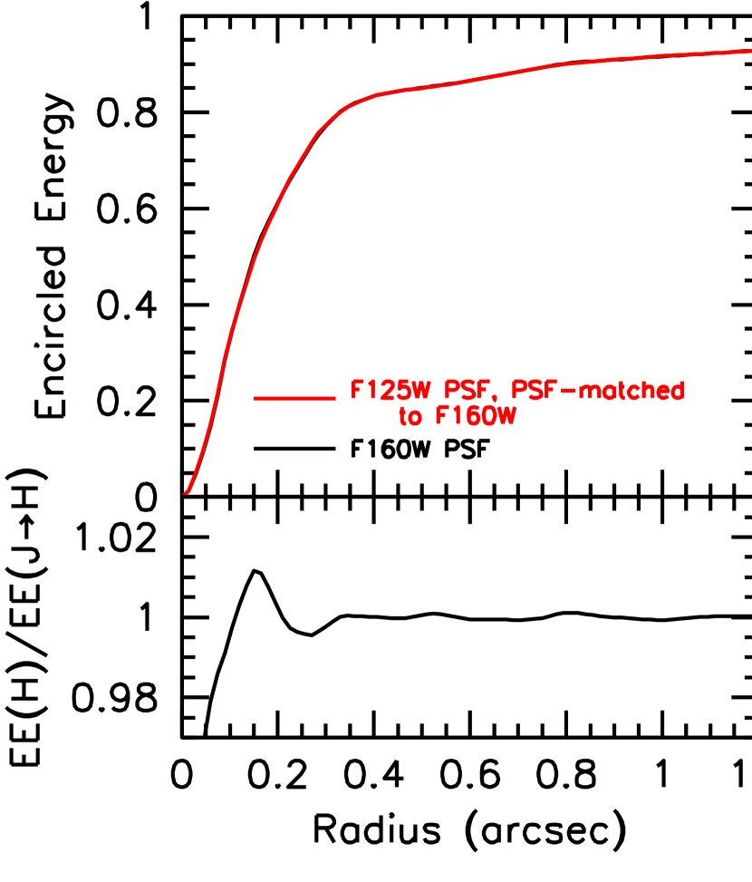
Figure 17.— (upper) Encircled-energy distribution for our $H_{160}$-band PSF (red line) and the $J_{125}$-band PSF (after PSF-matching to our $H_{160}$-band data: black line). (lower) Ratio between the encircled-energy distributions for the $H_{160}$-band PSF and our $J_{125}$-band PSF, after PSF-matching to the $H_{160}$-band data. The PSFs were matched so that the effective encircled-energy distributions would be identical in the two bands to $\lesssim 1.2$%. As a result, we would expect any systematic errors in our $\beta$ measurements to be smaller than $\Delta\beta\sim 0.05$ though we quote systematic errors of $\Delta\beta\sim\pm 0.13$ (3% accuracy on the colors) to be conservative.

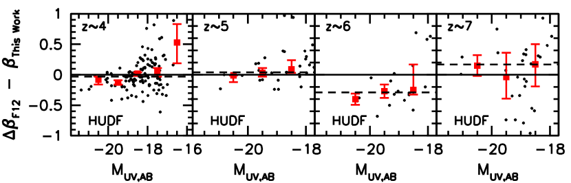
Figure 18.— Object-by-object differences (small black points) between the $\beta$’s we measure in this work with those measured in Finkelstein et al. (2012: F12) versus $UV$ luminosity ($M_{UV}$) for sources in our $z\sim 4$, $z\sim 5$, $z\sim 6$, and $z\sim 7$ samples from the XDF data set. When comparing against the Finkelstein et al. (2012) $\beta$ results, we have corrected their raw $\beta$ measurements (Table 3 of their work) for the $\Delta\beta\sim 0.23$ blueward bias in the faintest $z\sim 7$ galaxies they reported. The large red squares show the median differences in the measured $\beta$ for a bright subsample ($-21.5<M_{UV,AB}<-20$), an intermediate-magnitude subsample ($-20<M_{UV,AB}<-19$), and a fainter subsample ($-19<M_{UV,AB}<-18$). The dashed line gives the median difference in the measured $\beta$ for all sources in common between this work and that of Finkelstein et al. (2012). Good agreement is observed overall. Nevertheless, the $\beta$’s that Finkelstein et al. (2012) derive for the brightest $z\sim 4$ galaxies from the HUDF are slightly bluer (i.e., $\Delta\beta\sim 0.1$) than found here. Finkelstein et al. (2012) also measure slightly bluer $\beta$’s (i.e., $\Delta\beta\sim 0.2$) for $z\sim 6$ sources than we measure here. A similar offset in the $\beta$’s is apparent in comparing the $z\sim 6$ $\beta$ results from the ERS+CANDELS fields.

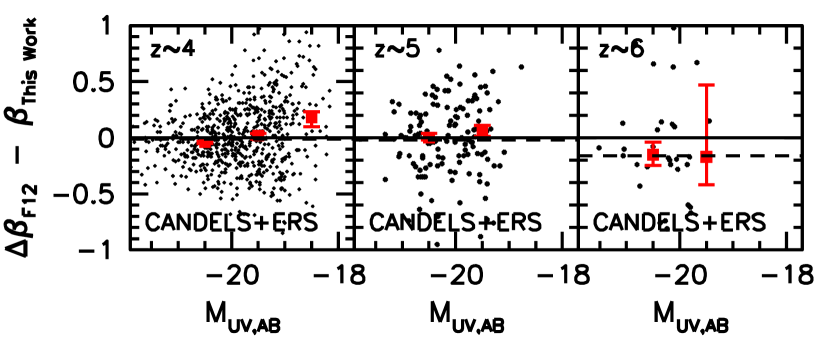
Figure 19.— Object-by-object differences (small black points) between the $\beta$’s we measure in this work with those measured in Finkelstein et al. (2012: F12) versus $UV$ luminosity ($M_{UV}$) for sources in our $z\sim 4$, $z\sim 5$, and $z\sim 6$ samples from the CANDELS-South and ERS data sets. The large red squares show the median differences in the measured $\beta$ for a bright subsample ($-21.5<M_{UV,AB}<-20$), an intermediate-magnitude subsample ($-20<M_{UV,AB}<-19$), and a fainter subsample ($-19<M_{UV,AB}<-18$). The dashed line gives the median difference in the measured $\beta$ for all sources in common between this work and that of Finkelstein et al. (2012). While the Finkelstein et al. (2012) results are in good agreement overall with our results, the derived $\beta$’s for the faintest sources in the CANDELS-South and ERS field from Finkelstein et al. (2012) are offset to redder values, by $\Delta\beta\sim 0.2$. As is discussed extensively in §4.7 of Bouwens et al. (2012), this likely occurs due to a coupling between the derived $\beta$’s for the faintest sources in the CANDELS-South field and the derived $UV$ luminosity of these sources.

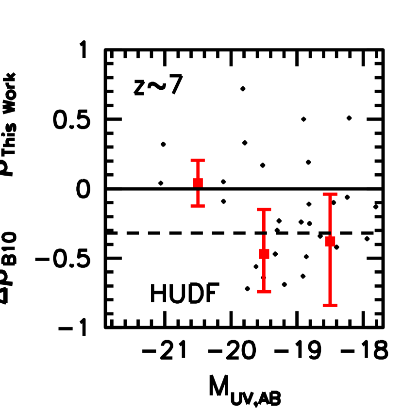
Figure 20.— Object-by-object differences (small black points) between the $\beta$’s we measure in this work and those measured in Bouwens et al. (2010: B10) versus $UV$ luminosity ($M_{UV}$) for sources in our $z\sim 7$ sample from the XDF data set. The results for $z\sim 7$ sources from our XDF data set can be shown (represented here as the small points) as often as twice, due to our selecting $z\sim 7$ sources on our fields twice (see §4.2). The large red squares show the median differences in the measured $\beta$ for a bright subsample ($-21.5<M_{UV,AB}<-20$), an intermediate-magnitude subsample ($-20<M_{UV,AB}<-19$), and a fainter subsample ($-19<M_{UV,AB}<-18$). The dashed line gives the median difference in the measured $\beta$ for all sources in common between this work and that of Bouwens et al. (2010). Differences between the present $\beta$ measurements and those of Bouwens et al. (2010) can be most easily explained as a result of a $\Delta\beta\sim 0.2$ systematic bias in the Bouwens et al. (2010) measurements (see Appendix B.2).

Appendix A A. Procedure to Obtain Accurate PSF-Matched Observations

Measurements of the $UV$-continuum slopes $\beta$ of galaxies are extremely sensitive to the color measurements. Even $\sim$0.05 mag errors in the measured colors result in $\Delta\beta\sim 0.12$-0.2 errors in the derived $\beta$’s (depending on how much leverage is available in wavelength). Accurate color measurements are therefore absolutely essential.

Great care has been taken in deriving accurate PSFs for each bandpass under study and in PSF-matching the multi-band observations. During the PSF-matching process, we explicitly verified that the encircled energy distribution for point sources in our observations were a good match to those from the $H_{160}$-band, after convolution by our PSF-matching kernel. Any residual systematics in the photometry of our PSF-matched observations should be no larger than 1.2%. Figure 17 illustrates the general quality of these results, comparing the encircled energy distribution for our $H_{160}$ PSF and that for our $J_{125}$ PSF, after PSF-matching the observations to the $H_{160}$ band. As is evident from the figure, the results are accurate to $\lesssim 1.2$%. Similar quality results are obtained in the PSF-matching the observations in the other passbands.

The real errors in the color measurements may be even larger than 1.2%, given that the HST zeropoints themselves are also uncertain (typically on the $\sim$1% level) as well as potential uncertainties in the amount of foreground extinction from our Galaxy. Considering all sources of error, we conservatively quote an uncertainty of 3% on our absolute color measurements (see §4.6). This translates into systematic uncertainties in our derived $\beta$’s of $\Delta\beta\lesssim 0.06$, $\Delta\beta\lesssim 0.08$, $\Delta\beta\lesssim 0.13$, and $\Delta\beta\lesssim 0.27$ at $z\sim 4$-5, $z\sim 6$, $z\sim 7$, and $z\sim 8$-8.5, respectively.

Appendix B B. Comparisons with Previous $\beta$ Measurements

To provide us with the broadest possible perspective on how our current $\beta$ measurements compare with previous published measurements, we conducted a comprehensive set of source-by-source comparisons with previous work. Not only did this provide us with an unparalleled view on how systematics could have affected previous studies, including our own, but it also provided us with valuable cross-checks on our results as we were putting together our samples and measurements.

B.1. B.1 Comparisons with the $\beta$ Measurements of Finkelstein et al. 2012

Independent of our own work on the $UV$-continuum slopes (Bouwens et al. 2009, 2010, 2012), the most comprehensive compilation of $\beta$ measurements in the literature has been provided by Finkelstein et al. (2012) for photometric-redshift-selected galaxy samples at $z\sim 4$, $z\sim 5$, $z\sim 6$, $z\sim 7$, and $z\sim 8$. Finkelstein et al. (2012) derived these $\beta$ measurements for these samples by fitting their photometry to model SEDs and then marginalizing over the results.

Figure 18 compares the $\beta$ measurements of Finkelstein et al. (2012) with those from the present work for sources from the XDF. For these comparisons, small corrections to the raw $\beta$ values provided by Finkelstein et al. (2012) consistent with the biases Finkelstein et al. (2012) estimate, the most significant of which is a $\Delta\beta\sim 0.23$ redward correction to the $\beta$ measurements for faint ($M_{UV,AB}\gtrsim-19$) $z\sim 7$ galaxies. A similar comparison is made for $\beta$ measurements from the CANDELS-South and ERS fields in Figure 19. The large solid squares show the median differences between the $\beta$ measurements from Finkelstein et al. (2012) and those obtained here.

The median $\beta$’s measured by Finkelstein et al. (2012) are $0.03_{-0.02}^{+0.02}$ bluer, $0.04_{-0.02}^{+0.07}$ redder, $0.29_{-0.13}^{+0.06}$ bluer, and $0.17_{-0.12}^{+0.08}$ redder for their $z\sim 4$, $z\sim 5$, $z\sim 6$, and $z\sim 7$ HUDF selections, respectively, than what we measure here. The median $\beta$’s derived by Finkelstein et al. (2012) for sources from the CANDELS-South and ERS fields are $0.01_{-0.02}^{+0.01}$ bluer, $0.02_{-0.03}^{+0.03}$ redder, and $0.16_{-0.13}^{+0.04}$ bluer at $z\sim 4$, $z\sim 5$, and $z\sim 6$, respectively, than the values we derive here.

Overall, the Finkelstein et al. (2012) $\beta$ results are in broad agreement with our own results, with a few noteworthy differences. At $z\sim 6$, the Finkelstein et al. (2012) $\beta$ measurements appear to be systematically bluer than our measurements on average, by $\Delta\beta\sim 0.2$. One possible cause for this difference is due to the effect of Ly$\alpha$ emission in boosting the broadband flux measurements at the position of the Lyman break. Since Finkelstein et al. (2012) use the flux information in all HST passbands in deriving $\beta$, it is possible this could shift their measured $\beta$’s to bluer values. Finkelstein et al. (2012) explicitly consider this type of effect in their paper and attempt to determine the impact it would have on their results. Finkelstein et al. (2012) report differences as large as $\Delta\beta\sim 0.25$ between the two approaches. The simulations shown by Rogers et al. (2013) also suggest that similar biases (i.e., $\Delta\beta\sim 0.25$-0.5) could be present in the Finkelstein et al. (2013) results due to Ly$\alpha$ emission.

The only other noteworthy difference we find is between the Finkelstein et al. (2012) $\beta$ results at $z\sim 4$ and our $\beta$ results. In particular, Finkelstein et al. (2012) measure bluer $\beta$’s for the brightest $z\sim 4$ sources than we measure and redder $\beta$’s for the faintest $z\sim 4$ sources. The effect is evident both in the results for the HUDF/XDF data set and from CANDELS-South and ERS data sets. The origin of this difference is not clear. However, since we find no median difference between the $\beta$’s we measure for the same $z\sim 4$ galaxies based on the XDF and the CANDELS-South data sets, we believe that it is unlikely to arise from our own measurements. By contrast, the median $\beta$’s that Finkelstein et al. (2012) derive for the faintest $z\sim 4$ sources from the CANDELS-South field and the HUDF differ by $\Delta\beta\gtrsim 0.2$ (disagreeing at $\sim 3\sigma$ significance).

One partial explanation for this offset is discussed in §4.7 of Bouwens et al. (2012: see also Finkelstein et al. 2012). We might expect small biases in the Finkelstein et al. (2012) $\beta$ vs. $M_{UV}$ results due to the fact that Finkelstein et al. (2012) determine the $UV$ luminosity of sources at approximately the same rest-frame wavelength as the blue end of the wavelength baseline they use to derive $\beta$. This effectively introduces a coupling between $M_{UV}$ and $\beta$, so that noise scatters sources either (1) to lower luminosities and redder $\beta$’s or (2) to higher luminosities and bluer $\beta$’s.

B.2. B.2 Comparisons with the $\beta$ Measurements of Bouwens et al. 2010

Much of the debate regarding the $UV$-continuum slopes $\beta$ of faint $z\sim 7$ galaxies has centered around the early measurements made by Bouwens et al. (2010), which were very blue, i.e., $\beta\sim-3$ (see also Finkelstein et al. 2010). These very blue measurements contrast with the $\beta$’s of $-2.30\pm 0.18$ we measure in this same general luminosity range $-19.3<M_{UV,AB}<-18.0$ from the XDF+HUDF09-Ps fields.

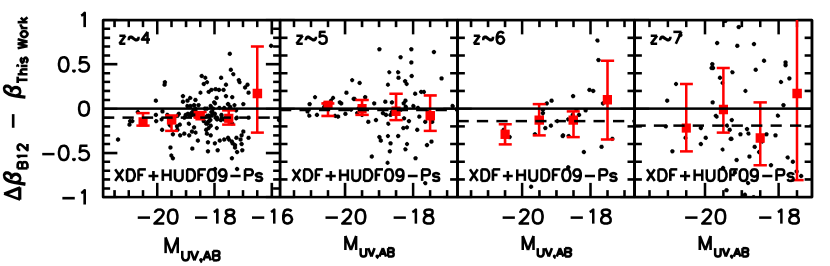
Figure 21.— Object-by-object differences (small black points) between the $\beta$’s we measure in this work with those measured in Bouwens et al. (2012: B12) versus $UV$ luminosity ($M_{UV}$) for sources in our $z\sim 4$, $z\sim 5$, $z\sim 6$, and $z\sim 7$ samples from the XDF data set. The large red squares show the median differences in the measured $\beta$ for a bright subsample ($-21.5<M_{UV,AB}<-20$), an intermediate-magnitude subsample ($-20<M_{UV,AB}<-19$), and a fainter subsample ($-19<M_{UV,AB}<-18$). The dashed line gives the median difference in the measured $\beta$ for all sources in common between this work and that of Bouwens et al. (2012). The sources considered here from Table 8 from Bouwens et al. (2012) were corrected for the relevant biases estimated in that study. The most important correction was a $\Delta\beta\sim 0.2$ redward offset to the $\beta$’s measured for the faintest $z\sim 7$ sources by Bouwens et al. (2012). In general, our current $\beta$ measurements are in good agreement with the Bouwens et al. (2012) measurements. However, we note a systematic bias in the Bouwens et al. (2012) $\beta$’s to bluer values. The size of this effect is $\Delta\beta\sim 0.1$, $\sim$0.0, $\sim$0.14, and $\sim$0.2 for $z\sim 4$, $z\sim 5$, $z\sim 6$, $z\sim 7$ sources. For the faintest galaxies in the Bouwens et al. (2012) $z\sim 7$ samples, the median $\beta$ may show a slightly larger offset relative to the present values. However, the difference is not statistically significant.

Why do the current results differ so significantly from the previous results? One factor is that Bouwens et al. (2010) required that sources in their $z\sim 7$ selection be detected at 5.5$\sigma$ in the $J_{125}$ band (Dunlop et al. 2012; Rogers et al. 2013). As a result, Bouwens et al. (2010) preferentially selected those $z\sim 7$ candidates which were brighter in the $J_{125}$ band (which can arise both as a result of the intrinsic color variations in galaxies and due to noise), causing the $J_{125}-H_{160}$ colors of their $z\sim 7$ candidates to be biased.

It is possible (at least approximately) to quantify the size of this bias by requiring that all sources in the $z\sim 7$, $-19<M_{UV,AB}<-18$ selection of Bouwens et al. (2010) also be detected at $5.5\sigma$ significance in the $H_{160}$-band, to mirror similar criteria applied in the $J_{125}$ band. As expected, the mean $\beta$ we measure for this $-19<M_{UV,AB}<-18$ subsample becomes somewhat redder as a result of imposing this additional criterion. However the change in the mean $\beta$ is only $\Delta\beta\sim 0.1$, i.e., from $\beta\sim-3$ to $\beta\sim-2.9$. This is somewhat surprising, since we might have expected to derive a somewhat larger bias in $\beta$ drawing on the Rogers et al. (2013) simulations albeit smaller in size than the bias predicted in Figure 6 of Rogers et al. (2013).

If noise-driven systematic biases were not the dominant explanation for differences with our current $\beta$ measurements, what is the explanation? Comparing the current $\beta$ measurements with those from Bouwens et al. (2010) on a source-by-source basis (Figure 20), we find some evidence for there being a systematic offset $\Delta\beta\sim 0.2$ offset between the $\beta$ measurements made in Bouwens et al. (2010) and those made here. Sources in both the two lowest-luminosity intervals show exactly the same offset in the median $\beta$ relative to the current measurements. Since we find essentially the same offset between the measured $\beta$’s from Bouwens et al. (2012) and the current study (Appendix B.2), this suggests the dominant bias in the reported $\beta$’s from Bouwens et al. (2010) may have been a systematic color measurement bias (see Figure 10) and that the role of noise-driven biases in producing the blue $\beta$’s may have been smaller.

Correcting for both effects gives us a mean $\beta$ of $\sim-2.68$, similar to the mean $\beta$ (i.e., $-2.18\pm 0.19$) we measure for sources in the luminosity interval $-19.3<M_{UV,AB}<-18$ from the current XDF data set.

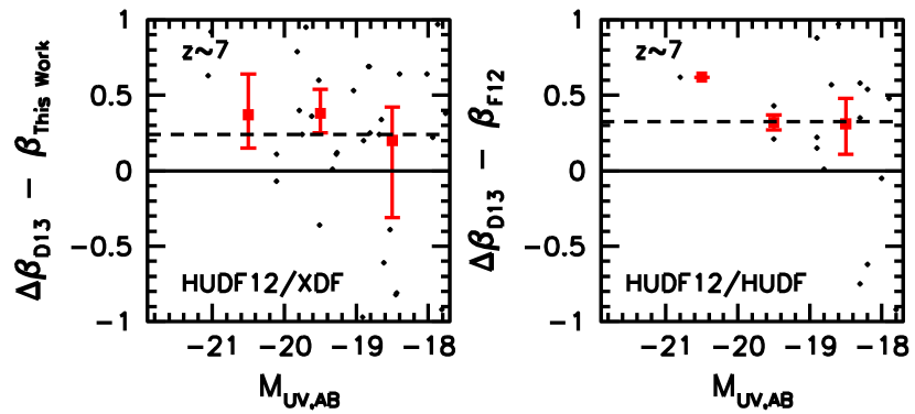
Figure 22.— (left) Object-object differences (small black points) between the $\beta$’s we measure in this work and those measured in Dunlop et al. (2013: D13) versus $UV$ luminosity ($M_{UV}$) for sources in our $z\sim 7$ sample from the HUDF12/XDF data set. The large red squares show the median differences in the measured $\beta$ for a bright subsample ($-21.5<M_{UV,AB}<-20$), an intermediate-magnitude subsample ($-20<M_{UV,AB}<-19$), and a fainter subsample ($-19<M_{UV,AB}<-18$). The dashed line gives the median difference in the measured $\beta$ for all sources in common between this work and Dunlop et al. (2013). Interestingly enough, the largest offsets between the $\beta$’s we derive and as derived by Dunlop et al. (2012) are for the brightest sources. The offsets for fainter sources are smaller. One would expect such a trend, if the Dunlop et al. (2013) $\beta$’s are biased redward in proportion to the size of the sources (see also Figure 11, §5.4, and Appendix D.4). (right) Similar to the left panel, except comparing the $\beta$’s measured by Finkelstein et al. (2012) with those measured in Dunlop et al. (2013) versus the $UV$ luminosity as determined by Finkelstein et al. (2012). $\Delta\beta\sim 0.23$ corrections to the individual $\beta$ measurements for the faintest sources in the Finkelstein et al. (2012) $z\sim 7$ sample were made to account the photometric error coupling bias that Finkelstein et al. (2012) estimated. Comparison of the Dunlop et al. (2013) results with those from Finkelstein et al. (2012) provide independent support for our general conclusion that the Dunlop et al. (2013) $\beta$ measurements are systematically biased to redder values (see also Figure 11).

B.3. B.3 Comparisons with the $\beta$ Measurements of Bouwens et al. 2012

The most comprehensive study of the $\beta$ distribution for $z\sim 4$-7 galaxies to date is that of Bouwens et al. (2012). Here we compare the present $\beta$ measurements we obtain for specific $z\sim 4$-7 galaxies in our XDF+HUDF09-Ps and ERS+CANDELS selections with those from Bouwens et al. (2012). This should allow us to determine very precisely the extent to which the $\beta$ measurements from Bouwens et al. (2012) exhibit any systematic offsets relative to those given here.

The object-by-object comparisons are shown in Figure 21 for sources in our XDF, HUDF09-Ps, ERS, and CANDELS selections. For these comparisons, small corrections to the raw $\beta$ values provided in Table 8 of Bouwens et al. (2012) are made. The most significant of these is a $\Delta\beta\sim 0.2$ redward correction to the $\beta$ measurements for faint ($M_{UV,AB}>-19$) $z\sim 7$ galaxies that Bouwens et al. (2012) found necessary to remove a noise-driven systematic bias (see §4.1).

While in general we find broad agreement between the $\beta$ measurements from our two studies, we note the presence of systematic offsets in the measured $\beta$’s. Compared to the present $\beta$ measurements for galaxies in our $z\sim 4$, $z\sim 5$, $z\sim 6$, and $z\sim 7$ samples over the XDF and HUDF09-Ps fields, those from Bouwens et al. (2012) are $\Delta\beta\sim 0.10_{-0.01}^{+0.02}$, 0.01${}_{-0.03}^{+0.03}$, 0.08${}_{-0.03}^{+0.08}$, and 0.19${}_{-0.14}^{+0.07}$ bluer, respectively, in the median than those derived in the present study. Comparing the Bouwens et al. (2012) $\beta$ results from CANDELS-South and the ERS field with those from the present work, we found that the median $\beta$’s derived by Bouwens et al. (2012) are $0.05\pm 0.01$ bluer, $0.10\pm 0.01$ bluer, $0.09_{-0.01}^{+0.03}$ bluer, $0.30_{-0.20}^{+0.06}$ bluer (in the median) at $z\sim 4$, $z\sim 5$, $z\sim 6$, and $z\sim 7$ than what we derive here.

While the above differences are consistent with the systematic uncertainties quoted by Bouwens et al. (2012) for their $\beta$ measurements, we do note a general shift in our measured $\beta$ values to redder values overall. The difference is most likely due to the Bouwens et al. (2012) PSFs not containing sufficient light in the wings due to their basing their PSFs on only a small sample of faint stars over the HUDF (for simplicity). If the PSFs for all passbands contained exactly the same amount of light in their wings, this would not significantly bias the Bouwens et al. (2012) results. However, given that the wings of the redder bandpasses contain more light than for the bluer passbands, this caused Bouwens et al. (2012) to measure colors which were systematically too blue. As a result, the $\beta$’s that Bouwens et al. (2012) derived are mildly bluer than measured here.

There was one additional potential bias regarding the Bouwens et al. (2012) study that was discussed by Dunlop et al. (2013) and developed further in Rogers et al. (2013). Rogers et al. (2013) show that the Bouwens et al. (2012) $\beta$ analysis would be biased blueward if Bouwens et al. (2012) had binned their selections as a function of the $J_{125}$-band magnitude in evaluating trends in $\beta$. However, this was not done by Bouwens et al. (2012), so it is unclear why Rogers et al. (2013) frame this as being potentially problematic for the Bouwens et al. (2012) study.

B.4. B.4 Comparisons with the $\beta$ Measurements of Dunlop et al. 2013

Finally, we consider the recent $\beta$ measurements obtained by Dunlop et al. (2013) for $z\sim 7$ galaxies in the HUDF12/XDF. The individual measurements of $\beta$ were obtained from Table A1 of their study.

B.4.1 B.4.1 Source-By-Source Comparisons

A comparison of the Dunlop et al. (2013) $\beta$ measurements with our own $\beta$ determinations is shown in Figure 22. Based on the plotted galaxies, we find a median offset of 0.24${}_{-0.06}^{+0.18}$ in the value of $\beta$, with the Dunlop et al. (2013) $\beta$’s being redder than those derived here. Such an offset in $\beta$ corresponds to a $\sim$0.06${}_{-0.02}^{+0.04}$ mag offset in the median $J_{125}-H_{160}$ color. A similar conclusion can be drawn comparing the Dunlop et al. (2013) results with those from Finkelstein et al. (2012: right panel of Figure 22).

B.4.2 B.4.2 Effect of the WFC3/IR Reductions on the $\beta$ Measurements

To investigate the origin of this offset, we first explored whether it could originate from the WFC3/IR reductions we were utilizing. We therefore downloaded the publicly available reductions the HUDF12 team made available to the community (Koekemoer et al. 2013), aligned this data set with our own, and then resampled these reductions onto the same grid as our own reductions of the HUDF12/HUDF09 WFC3/IR data set. We derived the effective PSF for the resampled Koekemoer et al. (2013) reductions, remeasured the fluxes for the sources using the same apertures, and rederived $\beta$ for all the sources in our $z\sim 7$ and $z\sim 8$ samples. The median $J_{125}-H_{160}$ colors we derive from the Koekemoer et al. (2013) reductions for $z\sim 7$ sources from our selections differ by just $\sim$0.01 mag (in the median) from those derived from our own reductions of the same data set. This suggests that the reductions themselves are not the source of the observed differences.

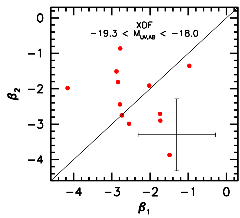
Figure 23.— A comparison of the two different $UV$-continuum slopes $\beta$ estimated for the same $-18.0<M_{UV,AB}<-19.3$ $z\sim 7$ candidates in the XDF (solid red circles). The $\beta$ on the horizontal axis ($\beta_{1}$) is estimated from the second $\sim$50% of the $J_{125}$ and $H_{160}$-band observations. The $\beta$ on the vertical axis ($\beta_{2}$) is estimated from the first 50% of the $J_{125}$ and $H_{160}$-band observations. Each of the two $z\sim 7$ selections contained one source that was not present in the other selection. A $1\sigma$ representative error bar is also shown. The difference between the two $\beta$ measurements are consistent with what one would expect from the uncertainties in the $J_{125}$ and $H_{160}$-band fluxes.

B.4.3 B.4.3 Effect of the Photometric Procedure of the $\beta$ Measurements

Next, we investigated whether the differences might originate from our procedures for performing photometry. We therefore measured $J_{125}-H_{160}$ colors for sources in our own $z\sim 7$-8 selection using the Dunlop et al. (2013) methodology for performing photometry. Dunlop et al. (2013) measure the $J_{125}$, $JH_{140}$, and $H_{160}$ fluxes for sources in 0.44^′′-diameter, 0.47^′′-diameter, and 0.50^′′-diameter circular apertures (with no PSF correction). Dunlop et al. (2013) have chosen these apertures for their photometry since these apertures enclose 70% of the light in the $J_{125}$, $JH_{140}$, and $H_{160}$-band images for point sources. [By comparison, we measure the fluxes of sources in identical Kron apertures, after PSF-correcting the HST observations to match the $H_{160}$-band observations.]

To investigate whether differences between the two photometric procedures could be the source of the differences between the reported $\beta$’s, we performed photometry on $z\sim 7$ sources in our selection using both procedures. Overall, we found similar $J_{125}-H_{160}$ colors using the two photometric procedures, but did nevertheless note a $\sim$0.03 mag median offset between the measured $J_{125}-H_{160}$ colors for sources in the luminosity range $-19<M_{UV,AB}<-18$.

B.4.4 B.4.4 Effect of Source Size on the Derived Color

Why would there be such differences between the measured colors? One potential explanation is that such differences could occur if the candidate $z\sim 7$ galaxies were not perfect point sources (as assumed by Dunlop et al. 2013) and in fact showed some spatial extension.

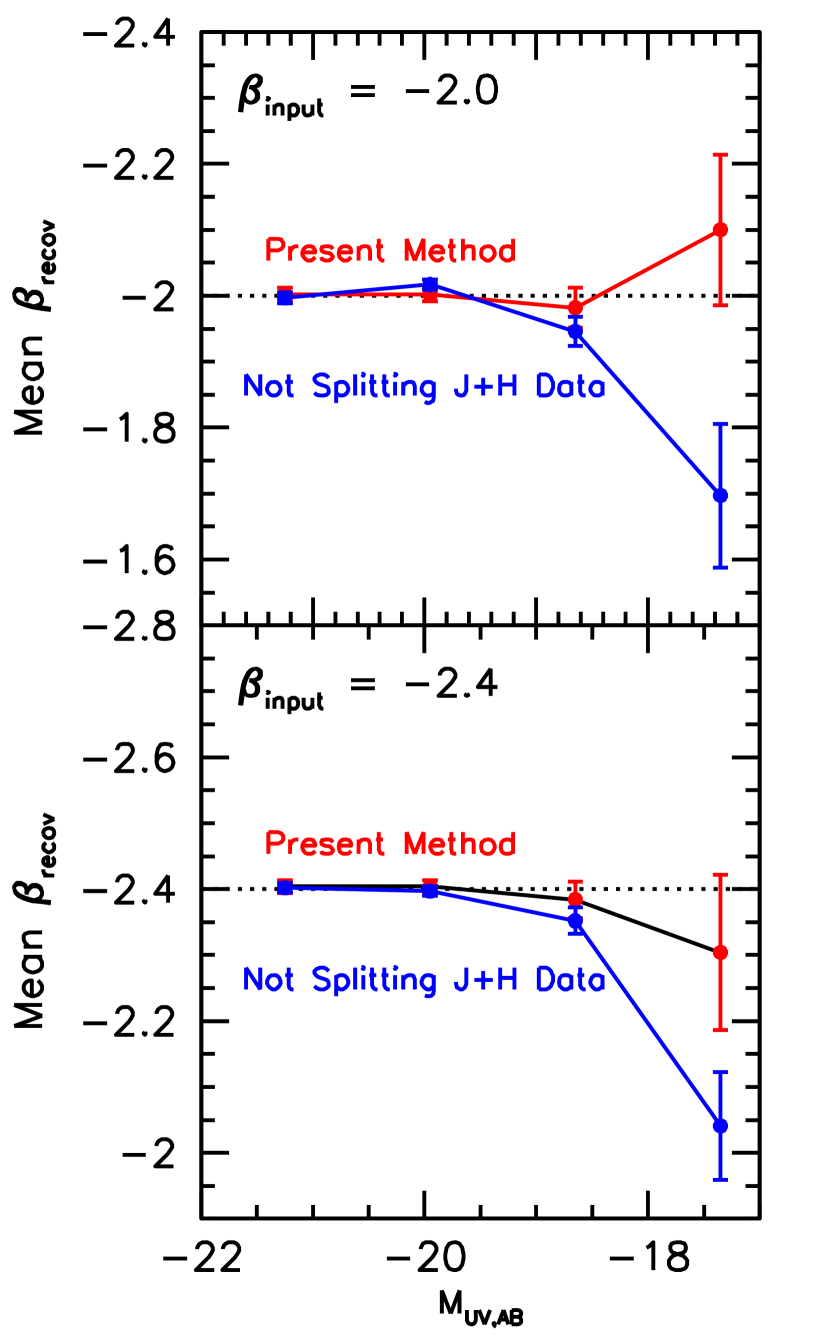
Figure 24.— The biweight mean $\beta$’s (red circles with $1\sigma$ errors) we recover versus $UV$ luminosity $M_{UV,AB}$ using a mock XDF data set and our proposed algorithm of splitting the $J_{125}$ and $H_{160}$-band exposures into two equal subsets and alternatively using one half of the observations to select sources and the other half to measure $\beta$. The error bars are derived from bootstrap resampling our results. The upper and lower panels show results assuming an input $\beta$ of $-2$ and $-2.4$, respectively, for all sources. Also shown (blue circles) are the biweight mean $\beta$’s adopting a procedure where the $J_{125}$ and $H_{160}$ data are not split into two equal subsets so as to separate the measurement of $\beta$ from the source selection process and the determination of $UV$ luminosity. In deriving these results, we used full end-to-end simulations, from the generation of images for mock galaxies and the selection of sources to the measurement of $\beta$. All of the mean $\beta$’s we derive from the simulations for our preferred algorithm (red circles) are within $1\sigma$ of the input values, strongly suggesting our final results should be free of significant systematic errors. This is in contrast to results for a procedure (blue circles) where the $J_{125}$ and $H_{160}$ data are not split into two equal subsets to separate the measurement of $\beta$ from source selection or the determination of the $UV$ luminosity.

To explore the effect the non-zero sizes of $z\sim 7$ galaxies have on the $J_{125}$ and $H_{160}$ band photometry, we stacked the $Y_{105}$, $J_{125}$, $JH_{140}$, and $H_{160}$-band images for all of the sources in the lower luminosity ($-19.3<M_{UV,AB}<-18$) $z\sim 7$ sample. We then constructed the encircled-energy distributions for this stacked source in the same way as we constructed this encircled-energy distribution for the five isolated stars we identified on the image. We find that the ratio of light in $0.50^{\prime\prime}$-diameter apertures to $0.44^{\prime\prime}$-diameter apertures is consistently $\sim$3% higher for faint ($-19.3<M_{UV,AB}<-18$) galaxies than it is for stars, independent of whether we consider stacks of the sources in the $Y_{105}$, $J_{125}$, $JH_{140}$, or $H_{160}$ bands.

Fitting for the half-light radius with galfit (Peng et al. 2002), we find a size of $0.074^{\prime\prime}$$\pm$0.013^′′, similar to the half-light radius (i.e., $\sim$0.06^′′ to 0.07^′′) measured by Ono et al. (2013). We checked that this size roughly reproduces the 3% differential excess observed for faint galaxies relative to stars. Computing the encircled energy distribution expected for sources with this radial profile and comparing with the results for sources with zero size, we calculate that sources with this half-light radius would be subject to a $\sim 0.03$ to 0.04 mag bias in their measured $J_{125}-H_{160}$ colors using the Dunlop et al. (2013) photometric scheme. Such a color bias would translate into a $\sim 0.13$-0.18 bias in $\beta$. Different source sizes, of course, translate into different expected biases in $\beta$. In Figure 11 from §5.4, we show how the bias in the $J_{125}-H_{160}$ colors and $\beta$ depends on the average half-light radii of sources under consideration (see also Figure 25 from Appendix E).

In addition, for $z\sim 7$ galaxies in the vicinity of other bright galaxies, it is also possible that the color measurements could be biased by light from neighboring sources. The wider 0.5^′′-diameter apertures (used for the $H_{160}$-band photometry) would include proportionally more light from neighboring sources than narrower $0.44^{\prime\prime}$-diameter apertures (used for the $J_{125}$-band photometry). While we would expect this effect to be small for typical sources, the systematic differences between different studies are on the 3-4% level and so even these types of effects could play a role.

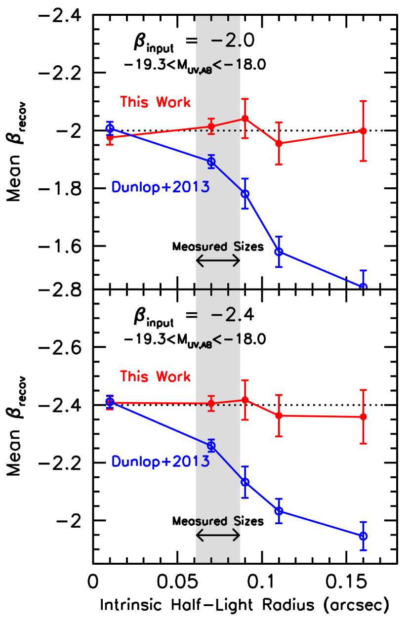
Figure 25.— The biweight mean $\beta$’s we recover (from full end-to-end simulations) versus the half-light radius of sources (solid red circles with $1\sigma$ errors) using our proposed algorithm on a mock XDF data. Also shown are the mean $\beta$’s we find using the photometric procedure of Dunlop et al. (2013: open blue circles with $1\sigma$ errors). The upper and lower panels show results assuming an input $\beta$ of $-2$ and $-2.4$, respectively, for all sources. The error bars are derived from bootstrap resampling our simulation results. While the mean $\beta$’s we derive are not significantly biased even in the case of large $z\sim 7$ galaxies, the mean $\beta$ one would derive using the photometric procedure that Dunlop et al. (2013) apply is biased towards redder $\beta$’s for large $z\sim 7$ galaxies (by $\Delta\beta\sim 0.5$). Since the faintest sources at $z\sim 7$ are nevertheless quite small, i.e., $r_{hl}=0.074\pm 0.013^{\prime\prime}$ (shaded grey region: see §5.4 and Appendix B.4), the actual bias in $\beta$ for faint $z\sim 7$ galaxies is modest but non-zero ($\Delta\beta\sim 0.13$ bias for faint $z\sim 7$ galaxies).

Appendix C C. Differences between the $\beta$ Measurements We Obtain using Two Independent Splits of the Observations

In this paper, we have presented an algorithm to obtain $\beta$ measurements for $z\sim 7$ samples in a way that is robust against noise-driven biases. We accomplish this by splitting our $J_{125}$ and $H_{160}$-band observations into two independent subsets and using one half of the observations for selecting individual sources and the other half for measuring $\beta$. The role of the two 50% splits of the data is then reversed.

While we were able to demonstrate that our procedure indeed allows to measure the mean $\beta$ for faint galaxy samples in a way that is robust against noise-driven biases (Appendix D), an important question is how such a procedure performs in practice for faint sources in real data sets. An example of this performance is illustrated in Figure 23 for faint $-19.3<M_{UV,AB}<-18.0$ galaxies from the XDF. Sources which are selected from both halves of the data set are shown at the horizontal and vertical values corresponding to their measured $\beta$ determinations in the first and second selections on each data set, respectively. Sources not selected in the first or second halves of the data set are plotted at zero on the vertical or horizontal axis, respectively.

From this figure, it is clear that for the luminosity interval chosen noise plays almost no role in moving individual $z\sim 7$ galaxies inside or outside of our $z\sim 7$ selection window. Essentially all $z\sim 7$ candidates are present in both selections. Moreover, the measured $\beta$’s from the two selections typically differ by less than $\Delta\beta\sim 0.8$. While these differences are modest, larger differences between the two selections are expected near the flux limit of the XDF data set.

Appendix D D. Realistic End-to-End Simulations Demonstrating that Our New Algorithm is Robust Against Noise-Driven Biases

In the main text of this paper, we have described a new algorithm for measuring $\beta$ for $z\sim 7$ galaxies that is robust against noise-driven biases. This approach is valuable in cases where data are available in only three near-infrared filters, since this would normally lead to systematic errors from the crosstalk between color information needed for redshift determination and that needed to determine $\beta$. We demonstrate here the effectiveness of this approach using realistic end-to-end simulations.

We assume that all galaxies have exactly the same intrinsic SED – which we take to be a perfect power-law spectrum with $\beta=-2$. We assume there are an equal number of galaxies at ten discrete redshifts, $z=6.2$, $z=6.4$, …, $z=7.6$, and at five apparent magnitudes in the $H_{160}$ band $H_{160,AB}=27.5$, $H_{160,AB}=28$, $H_{160,AB}=28.5$, $H_{160,AB}=29.0$, and $H_{160,AB}=29.5$ (before adding noise). We include the effect of opacity from the neutral hydrogen forest following the Madau (1995) prescription, with no transmittance at redshifts higher than $z=6$.

Based on this intrinsic SED and opacity model, we calculate the flux of sources in the $z_{850}$, $Y_{105}$, $J_{125}$, and $H_{160}$ bands. We then simulated 11 different images of each model galaxy, including one image each for the $B_{435}V_{606}i_{775}I_{814}z_{850}Y_{105}JH_{140}$ bands and two equal-depth images for the $J_{125}$ and $H_{160}$ bands. We assume that the half-light radius distribution of galaxies is equally divided between galaxies with 0.01^′′, 0.06^′′, 0.11^′′, and 0.16^′′ radii. Axial ratios for sources were assumed to be uniformly distributed between 1.0 and 1.5. Simulated sources were then convolved with our derived PSFs in the different passbands (§2.2 and Appendix A) and noise added to match that present in the XDF data set. 100 galaxies were included per arcmin² on the simulated images.

We then selected and measured $\beta$ for individual sources using exactly the same procedure as we applied on the XDF data set itself (and other data sets in this study: see §4.3). The biweight mean $\beta$’s we derive assuming an input $\beta$ of $-2$ and $-2.4$ is shown in Figure 24, and it is clear that our procedure works very well in recovering the input $\beta$’s. The procedure we use to derive the biweight mean $\beta$ is the same, as what we use on the observations themselves. $3\times$10⁴ sources are used in these simulations.

We also present our recovered biweight mean $\beta$’s using a simpler procedure where the $J_{125}$ and $H_{160}$ band data are not split into two equal pieces. In this case, the same $J_{125}$ and $H_{160}$-band flux measurements are used for source selection, the measurement of $\beta$, and the determination of the $UV$ luminosity. Whereas our preferred algorithm shows a bias consistent with zero, this alternate algorithm (i.e. using the same $J_{125}$ and $H_{160}$-band flux measurements for all three processses which is the most direct approach) shows a small but clear bias.

Appendix E E. The Sensitivity of the Derived $\beta$’s to Source Size Using the Present Approach and the Dunlop et al. (2013) Photometric Procedure

As we emphasized in §5.4, the $\beta$’s one derives for $z\sim 7$ galaxies can be biased by the sizes of $z\sim 7$ galaxies and the assumptions one’s photometric procedure makes about these sizes. Since we ensure that our observations are PSF-matched before we perform our photometry, we would not expect our measured $\beta$’s to be affected by the size of $z\sim 7$ galaxies. By contrast, Dunlop et al. (2013) derive colors for sources in apertures containing 70% of the light for point sources (0.44^′′-diameter apertures in the $J_{125}$ band, 0.47^′′-diameter apertures in the $JH_{140}$ band, and 0.50^′′-diameter apertures in the $H_{160}$ band). Adopting the latter approach can result in biased measurements of the $J_{125}-H_{160}$ colors if $z\sim 7$ galaxies are not in fact point sources.

We can use the same set of simulations as we used in the previous section to test the dependence of the robustness of our $\beta$ measurements on the size of sources. We will also use these same simulations to test the dependence of the $\beta$ measurements on source size, if we adopt the Dunlop et al. (2013) photometric procedure. We focus on the results in the magnitude interval $-19.3<M_{UV,AB}<-18.0$, since this has been the focus of the controversy.

In upper and lower panels of Figure 25, we show how the mean $\beta$ we measure depends on the half-light radius of sources, assuming an input $\beta$ of $-2$ and $-2.4$ in the simulations. In both cases, we are able to recover the mean $\beta$’s to which the quoted uncertainties over the full range of source sizes $0.01^{\prime\prime}$ to $0.16^{\prime\prime}$. On the same figure, we also plot the mean $\beta$’s we derive using the Dunlop et al. (2013) photometric procedure, again as a function of the size of $z\sim 7$ galaxies input into the simulations. Again, while the Dunlop et al. (2013) photometric procedure is successful at recovering $\beta$ quite accurately for small ($\sim$0.01^′′) sources, we find a redward bias in the measured $\beta$ as the size of the source increases. For sources with half-light radii of $\sim$0.15^′′, we find that that the derived $\beta$’s are too red by $\Delta\beta\sim 0.5$. Our results here are in contrast to those from Dunlop et al. (2013), who conclude based on the end-to-end testing they run that there is no bias in the $\beta$’s they measure for $z\sim 7$ galaxies. The conclusion of Dunlop et al. (2013) is incorrect because they model faint $z\sim 7$ galaxies as point sources in their simulations, and as shown here and by Ono et al. (2013), this is not an accurate assumption to make.

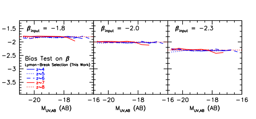
Figure 26.— Estimated mean $\beta$ we would recover as a function of the $UV$ luminosity of sources due to the fact that galaxies with intrinsically bluer $\beta$’s are more selectable than galaxies with redder $\beta$’s (see Appendix F). The input $\beta$ distribution for these simulations is assumed to have a mean value of $\beta=-1.8$ (left), $\beta=-2.0$ (center), and $\beta=-2.3$ (right), with a $1\sigma$ scatter of 0.35. Similar simulations were performed in Appendix B.1.1 of Bouwens et al. (2012). Shown are the results for our $z\sim 4$, $z\sim 5$, $z\sim 6$, $z\sim 7$, and $z\sim 8$ selections over the XDF data set. The typical bias in $\beta$ is $\Delta\beta\lesssim 0.05$ for our selection criteria.

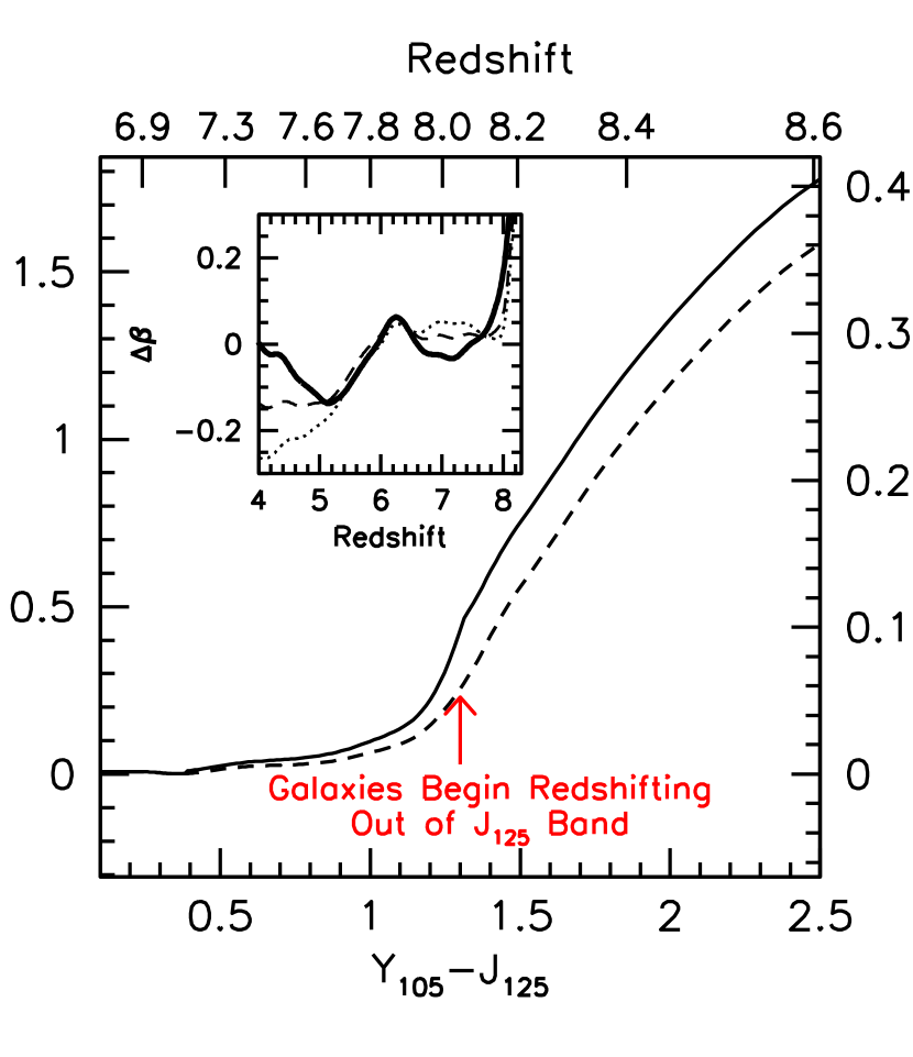
Figure 27.— Estimated correction (solid line) that must be made to the observed spectral slopes for $z\sim 8$ galaxies inferred from the $J_{125}-H_{160}$ colors. The correction is relative to the intrinsic $\beta$ for the model SED under consideration, which is calculated from the 1270Å to 2600Å wavelength range traditionally used to define $\beta$ (Calzetti et al. 1994). The required correction to $\beta$ is a function of the redshift of a galaxy, which can be approximately computed based on the $Y_{105}-J_{125}$ color. Corrections are necessary to account for two effects: (1) the redshifting of galaxies out of the $J_{125}$-band at $z\gtrsim 8.1$ (resulting in substantially redder $J_{125}-H_{160}$ colors), (2) the impact of the Ly$\alpha$ damping wing on the observed colors, and (3) the somewhat redder shape of the SED blueward of 1350Å. The net results of the three effects is that, if uncorrected, galaxies would appear to have redder $UV$-continuum slopes $\beta$ at $z\sim 8$ than at $z\sim 7$, even if there is no evolution. The Ly$\alpha$ damping wing is computed assuming a $10^{21}$ cm² neutral hydrogen column and a $x_{e}=0.2$ neutral fraction in the IGM. The dashed line shows the correction not accounting for the Ly$\alpha$ damping wing. The figure inset shows how the correction depends on the precise shape of the SED for a star-forming galaxy and is shown over a larger range in redshift. The dashed, dotted, and thick solid curves give the corrections assuming (1) a $10^{8}$ year constant star formation model, (2) a 10-Myr constant star formation model, and (3) an $80$-Myr constant star formation model followed by 20-Myr with no star formation. The correction to $\beta$ that we utilize is the average of models (1) and (3). Dunlop et al. (2013) do not discuss correcting the $\beta$’s they derive at $z\sim 8$ for the effect of the IGM on the $J_{125}$-band fluxes. While this effect will not have a huge impact on the derived $\beta$’s from Dunlop et al. (2013), we do estimate a redward bias of $\Delta\beta\sim 0.1$ using the redshift distribution that Dunlop et al. (2013) provide for their $z\sim 8$ sample.

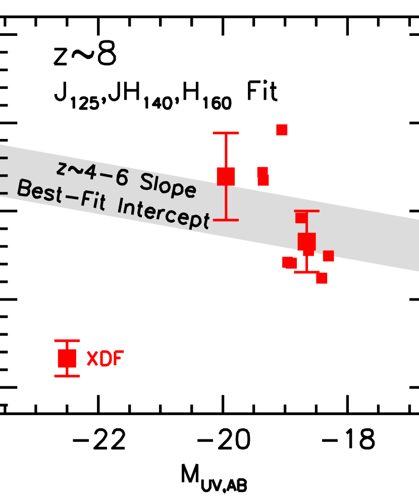
Figure 28.— Measured $\beta$’s (small red squares) versus the rest-frame $UV$ luminosity $M_{UV}$ for galaxies in our XDF sample of $z\sim 8$ galaxy candidates (see Appendix G.2). The $\beta$’s we derive for sources here are based on a power-law fit to the $J_{125}$, $JH_{140}$, and $H_{160}$ photometry, in contrast to Figure 12 where we present our results for our XDF sample based on a power-law fit to the $JH_{140}$ and $H_{160}$ photometry. The large red squares represent the inverse-variance-weighted mean $\beta$’s and $1\sigma$ uncertainties, in various 1.3-mag bins of $UV$ luminosity. The gray-shaded band shows the $1\sigma$ range allowed for a fit to the $\beta$-$M_{UV}$ relation fixing the slope of this relation to the average value ($-0.13$) found by Bouwens et al. (2012) for $z\sim 4$-6 galaxies.

Appendix F F. Computing the “Selection Volume Bias”: Bias Related to the Intrinsic Selectability of Sources

All photometric criteria used to identify high-redshift galaxies, whether it be a traditional Lyman-Break selection or a simple photometric redshift approach, are much more effective in the selection of sources with bluer spectral slopes than in the selection of sources with redder slopes. As a result, the bluest galaxies at high redshifts will be overrepresented in high-redshift samples relative to the reddest galaxies (proportionally speaking), resulting in a biased measurement of the mean $\beta$ in high-redshift samples, if one does not control for these effects.

In general, the bias in the $\beta$ one derives will be quite large, if the information one uses to derive $\beta$ is not independent of the information one uses to select sources. In this situation, noise can drive both the selection of sources and the measurement of $\beta$, resulting in potentially large biases in $\beta$. Such a scenario is extensively discussed by Bouwens et al. (2012) and Dunlop et al. (2012) and has been called the photometric error coupling bias by Bouwens et al. (2012: see Appendix B.1.2 from that work).

As a result of such concerns, great care has been taken here to ensure that the $\beta$ measurements reported here are entirely decoupled from the selection process (and for the definition of the photometric apertures) for the faintest sources in all of our high redshift samples. This ensures, by construction, that the photometric error coupling bias is identically zero.

However, one can still arrive at a biased measurement of the mean $\beta$, even if one measures their mean $\beta$ using independent information from what one uses to select high-redshift sources. This is as a result of the fact that sources with intrinsically bluer colors are selected more efficiently than those with redder colors.

To compute the size of this bias for our $\beta$ results, we added artificial sources to the real observations over a wide range in $\beta$ (i.e., $\beta=-4$ to $\beta=2$), $UV$ luminosity, and redshift. To simulate the spatial profiles of individual sources we added to the real data, we made use of similar-luminosity $z\sim 4$ galaxies from the XDF data set and artificially redshifted them using our “cloning” machinery (Bouwens et al. 1998; Bouwens et al. 2003) to a range of redshifts over the selection window of our high-redshift samples, scaling their physical sizes as $(1+z)^{-1}$ to match the observed scalings (e.g., Bouwens et al. 2006; Oesch et al. 2010; Mosleh et al. 2012). After adding the sources to the real data, we then attempted to reselect the sources using the same procedure as we apply to the real observations, and we computed the selection efficiency of galaxies as a function of their $UV$ luminosity and their intrinsic $\beta$.

Then, using the selection efficiency results from the above simulations and assuming that the inherent $\beta$’s for $z\sim 4$-8 galaxies is normally distributed with some mean value and a standard deviation $\sigma_{\beta}\sim 0.35$ (consistent with that derived by Bouwens et al. 2009; Bouwens et al. 2012; Castellano et al. 2012), we have calculated the bias in $\beta$. The results are shown in Figure 26. In general, the bias we expect in $\beta$ is not especially large, $\Delta\beta\lesssim 0.05$, and should not appreciably bias the results for all three input $\beta$’s we have considered, i.e., $\beta\sim-1.8$, $\beta\sim-2.0$, and $\beta\sim-2.3$. While the computed bias could be quite a bit larger if the intrinsic $\beta$ distribution were larger, recent results by Rogers et al. (2014) not only confirm that the intrinsic width of the $\beta$ distribution is $\sim$0.35, but provide evidence that the width of this distribution is even narrower for lower luminosity sources. This strongly suggests that any biases resulting from differences in the intrinsic selectability of sources should be small, i.e., $\Delta\beta\lesssim 0.05$. Similar simulations were previously presented in Appendix B.1.1 of Bouwens et al. (2012).

Appendix G G. $\beta$ Determinations for $z\sim 8$ Galaxies by Fitting to the Measured $J_{125}+JH_{140}+H_{160}$ Fluxes

G.1. G.1 General Procedure

Our primary method for deriving $\beta$ at $z\sim 8$ only makes use of the flux measurements in the $JH_{140}$ and $H_{160}$ bands. The advantage of this approach is that for both bands, the full wavelength coverage lies firmly in the $UV$-continuum and redward of the Lyman break, and therefore the $JH_{140}-H_{160}$ color provides a reliable measurement of the $UV$ slope $\beta$. One significant drawback, however, in restricting ourselves to the use of these bands in deriving $\beta$ is the limited leverage in wavelength the two bands provide for determining $\beta$, resulting in much larger statistical uncertainties in the derived $\beta$’s.

Fortunately, one can consider making use of the observed $J_{125}$-band flux to gain additional leverage for constraining the $UV$-continuum slope $\beta$. The challenge with including $J_{125}$-band flux measurements in the fits is that both Ly$\alpha$ and the Lyman break begin to enter the $J_{125}$ band at $z\gtrsim 8.1$ (see Figure 27). This can significantly bias the measured $\beta$’s for individual $z\sim 8$ sources if this effect is not corrected for. The Lyman break would make $z\sim 8$ galaxies too faint in the $J_{125}$-band relative to the baseline continuum values, while Ly$\alpha$ emission would make the $J_{125}$-band fluxes too bright. While one might imagine that this issue would be isolated to only those sources with redshift estimates in excess of 8.0, the redshift of each source in our $z\sim 8$ sample is uncertain and so could potentially be in excess of 8 (and therefore be biased by this issue, if not corrected). Corrections for IGM absorption can also be somewhat model dependent. It is because of these challenges that we opted not to use this as our primary approach.

In order to overcome these issues and still make use of the observed $J_{125}$-band fluxes to derive $\beta$, it is clear that a correction to the $J_{125}$-band fluxes of $z\sim 8$ sources is required. Here we estimate the approximate effect the Lyman-break has on the $J_{125}$-band flux based on the redshifts we infer for sources using their measured $Y_{105}-J_{125}$ colors. Three different SED templates are considered in correcting the $J_{125}$-band fluxes for $z\sim 8$ galaxies in our samples: the first assuming constant star formation for 100 Myr, the second assuming constant star formation for 10 Myr, and the third assuming constant star formation for $80$ Myr followed by 20 Myr with no star formation. Different star formation histories were explored to see what effect the shape of the $UV$-continuum has on the derived $UV$-continuum slopes. SED templates were derived for each of these star-formation histories using the Bruzual & Charlot (2003) spectral synthesis code and 0.2 $Z_{\odot}$ metallicities. From the inset of Figure 27, it is clear that the unknown star-formation histories for individual sources could have a modest effect on the results. The $\beta$ corrections we adopt are taken to be an average of the results for the first and third model star-formation histories.

The observed $J_{125}$-band fluxes for $z\sim 8$ galaxies are also attenuated somewhat due to damped absorption from neutral hydrogen gas in the galaxy and likely an increasingly neutral IGM. Assuming a neutral hydrogen column of $\sim$1$\times$10²¹ cm^-2 in individual galaxies, we estimate that the Ly$\alpha$ damping wing could attenuate the $J_{125}$-band flux seen from individual sources by $\sim$2-3%. We also account for some absorption from neutral hydrogen in the IGM (Miralda-Escude 1998), assuming a neutral fraction $x_{e}$ of 0.2 at $z\sim 8$ (Bouwens et al. 2012; Kuhlen & Faucher-Giguere 2012; Robertson et al. 2013). The observed $J_{125}$-band fluxes are corrected for this effect based on the redshifts we infer for sources from their $Y_{105}-J_{125}$ colors.

Accounting for the effect of Ly$\alpha$ emission on the observed $J_{125}$-band fluxes would also be useful. However, spectroscopic follow-up of current $z\sim 7$-8 samples (e.g., Ono et al. 2012; Schenker et al. 2012; Pentericci et al. 2011; Caruana et al. 2012) seems to suggest that Ly$\alpha$ emission is quite rare in these sources (likely due to an increasingly neutral medium). Therefore, we would not expect Ly$\alpha$ emission to have a large effect on the observed colors. If this is not the case for all sources, this could bias the measurements.

This second approach to deriving $\beta$ for $z\sim 8$ galaxies is very similar to one recently utilized by Dunlop et al. (2013) in examining the spectral slopes of $z\sim 8$ galaxies over the HUDF12. However, Dunlop et al. (2013) appear to have made no correction to the $J_{125}$-band fluxes used in their fits, since this issue is not discussed in their paper. Using the redshift distribution Dunlop et al. (2013) estimate for their $z\sim 8$ sample (Appendix A of Dunlop et al. 2013), we estimate that the bias in $\beta$ will be $\sim 0.1$ to the red. While this bias is likely not huge (and here we assume that the contribution from Ly$\alpha$ emission is not substantial), it will cause the $\beta$’s inferred by Dunlop et al. (2013) to be slightly redder than what we find in §6.2 (at least for the $z\sim 8$ $\beta$’s they derive from the $J_{125}-H_{160}$ colors).

G.2. G.2 Results for $z\sim 8$ Sample

In this section, we apply the approach we describe in the previous section to the three deepest HST fields to derive the mean $\beta$ for faint $z\sim 8$ galaxies. For consistency with our primary $\beta$ determinations for $z\sim 8$ galaxies in §6, we use the same criteria for selecting $z\sim 8$ galaxies as given in §6.1. There we derived the mean $\beta$ based on a small $z\sim 8$ sample from the XDF data set using a power-law fit to the $JH_{140}$ and $H_{160}$-band fluxes.

Similar to the strategy we employ on our $z\sim 7$ samples, we split the $J_{125}$-band observations into two equal subsets and alternatively select and measure $\beta$ on each half of the data. This is to ensure that our results are not biased due to a coupling between the $J_{125}$-band flux used to derive $\beta$ and that used to select the sources. Given the sensitivity of our results to having accurate $Y_{105}-J_{125}$ colors for candidates in our $z\sim 8$ (see Figure 27), we restrict our analysis to only those sources from the XDF data set in determining the mean $UV$-continuuum slopes $\beta$.

We plot the observed $\beta$’s for individual sources in Figure 28 as a function of their measured luminosities. Subdividing our $z\sim 8$ sample by $UV$ luminosity, we derive the inverse-variance-weighted mean $\beta$’s for sources in each luminosity bin. The results are then presented in Figure 28 as the large blue squares. The inverse-variance-weighted mean $\beta$ in the luminosity interval $-19.3<M_{UV,AB}<-18.0$ is $-2.39\pm 0.35\pm 0.13$. This determination is quite consistent with the $\beta$ for derive for $z\sim 8$ in a similar luminosity interval in §6.2, i.e., $-$1.88$\pm$0.74$\pm$0.27. While it might seem surprising that our determination using the full $J_{125}+JH_{140}+H_{160}$ flux information is bluer than the determination from §6.2 given what was argued about the impact of the IGM on the $J_{125}$ flux for $z\gtrsim 8$ sources, we emphasize that the $z\sim 8$ $\beta$’s we derive in this section are based on $J_{125}$-band fluxes corrected for the impact of the IGM.

Finally, we fit the $\beta$ vs. $M_{UV}$ relationship to a line, fixing the slope of this relationship to the average slope found for $z\sim 4$-6 galaxies by Bouwens et al. (2012), i.e., $-0.15$. The best-fit intercept for this relationship at $M_{UV}$ luminosity of $-19.5$ mag is $-2.01\pm 0.28\pm 0.13$. This value is in excellent agreement with that given in §6.2.

Appendix H H. Complete Set of $\beta$ and $M_{UV}$ Measurements for Our $z\sim 4$-8 Samples

To facilitate comparisons with the present results (and in the interests of transparency), we provide a complete list of the sources in our $z\sim 4$, $z\sim 5$, $\sim 6$, $z\sim 7$, and $z\sim 8$ samples in Table 8. This table includes the coordinates of the sources as well as their derived $\beta$’s and $UV$ luminosities ($M_{UV}$). A complete set of the flux measurements used to derive $\beta$ for these sources is provided in Table 9.

Table 8A complete list of the UV-continuum slopes $\beta$ we measure for sources in our $z\sim 4$, $z\sim 5$, $z\sim 6$, $z\sim 7$, and $z\sim 8$ samples

Source ID	R.A.	Declination	$M_{UV,AB}$	$\beta$	$<z>$	Data Set
XDF-23876748271	03:32:38.76	$-$27:48:27.11	$-$19.54	0.00$\pm$0.14	4	1
XDF-23848748246	03:32:38.49	$-$27:48:24.64	$-$16.54	$-$3.00$\pm$1.42	4	1
XDF-23848748214	03:32:38.49	$-$27:48:21.44	$-$17.92	$-$1.82$\pm$0.22	4	1
XDF-23842748186	03:32:38.42	$-$27:48:18.69	$-$16.45	$-$2.40$\pm$0.55	4	1
XDF-23796748182	03:32:37.96	$-$27:48:18.22	$-$16.00	0.36$\pm$1.32	4	1
XDF-23766748168	03:32:37.66	$-$27:48:16.88	$-$17.24	$-$2.08$\pm$0.35	4	1
XDF-23800748165	03:32:38.00	$-$27:48:16.51	$-$19.14	$-$1.16$\pm$0.13	4	1
XDF-23884748189	03:32:38.84	$-$27:48:18.97	$-$20.24	$-$0.95$\pm$0.12	4	1
XDF-23859748162	03:32:38.60	$-$27:48:16.23	$-$18.06	$-$2.01$\pm$0.23	4	1
XDF-23836748145	03:32:38.37	$-$27:48:14.51	$-$15.84	$-$3.07$\pm$1.96	4	1

Table 9Complete set of flux measurements used to derive $\beta$ for our $z\sim 4$, $z\sim 5$, $z\sim 6$, $z\sim 7$, and $z\sim 8$ samples

	Measured Flux (100 pJy)
Source ID	$i_{775}$	$I_{814}$	$z_{850}$	$Y_{098}$	$Y_{105}$	$J_{125}$	$JH_{140}$	$H_{160}$
XDF-23876748271	760$\pm$24	827$\pm$66	871$\pm$40	—	—	1862$\pm$42	—	—
XDF-23848748246	62$\pm$15	$-$28$\pm$42	13$\pm$25	—	—	40$\pm$26	—	—
XDF-23848748214	211$\pm$11	198$\pm$32	235$\pm$19	—	—	216$\pm$18	—	—
XDF-23842748186	60$\pm$9	29$\pm$24	61$\pm$15	—	—	48$\pm$13	—	—
XDF-23796748182	11$\pm$10	26$\pm$26	27$\pm$16	—	—	52$\pm$17	—	—
XDF-23766748168	112$\pm$11	133$\pm$30	99$\pm$19	—	—	111$\pm$18	—	—
XDF-23800748165	578$\pm$11	594$\pm$32	698$\pm$19	—	—	823$\pm$18	—	—
XDF-23884748189	1545$\pm$12	1550$\pm$34	1866$\pm$21	—	—	2430$\pm$19	—	—
XDF-23859748162	247$\pm$15	213$\pm$42	286$\pm$26	—	—	259$\pm$23	—	—
XDF-23836748145	25$\pm$9	17$\pm$24	24$\pm$14	—	—	7$\pm$13	—	—

References

- Alavi et al. (2014) Alavi, A., Siana, B., Richard, J., et al. 2014, ApJ, 780, 143
- Beckwith et al. (2006) Beckwith, S. V. W., et al. 2006, AJ, 132, 1729
- Beers et al. (1990) Beers, T. C., Flynn, K., & Gebhardt, K. 1990, AJ, 100, 32
- Bouwens, Broadhurst and Silk (1998) Bouwens, R., Broadhurst, T. and Silk, J. 1998, ApJ, 506, 557
- Bouwens et al. (2003) Bouwens, R., Broadhurst, T., & Illingworth, G. 2003, ApJ, 593, 640
- Bouwens et al. (2006) Bouwens, R.J., Illingworth, G.D., Blakeslee, J.P., & Franx, M. 2006, ApJ, 653, 53
- Bouwens et al. (2007) Bouwens, R. J., Illingworth, G. D., Franx, M., & Ford, H. 2007, ApJ, 670, 928
- Bouwens et al. (2009) Bouwens, R. J., et al. 2009, ApJ, 705, 936
- Bouwens et al. (2010) Bouwens, R. J., Illingworth, G. D., Oesch, P. A., et al. 2010, ApJ, 709, L133
- Bouwens et al. (2011) Bouwens, R. J., Illingworth, G. D., Oesch, P. A., et al. 2011, ApJ, 737, 90
- Bouwens et al. (2012) Bouwens, R. J., Illingworth, G. D., Oesch, P. A., et al. 2012, ApJ, 754, 83
- Bouwens et al. (2012) Bouwens, R. J., Illingworth, G. D., Oesch, P. A., et al. 2012a, ApJ, 752, L5
- Bouwens et al. (2013) Bouwens, R., Bradley, L., Zitrin, A., et al. 2013, ApJ, submitted, arXiv:1211.2230
- Bouwens et al. (2014) Bouwens, R. J., Illingworth, G. D., Oesch, P. A., et al. 2014, arXiv:1403.4295
- Bromm & Larson (2004) Bromm, V., & Larson, R. B. 2004, ARA&A, 42, 79
- Bruzual & Charlot (2003) Bruzual, G., & Charlot, S. 2003, MNRAS, 344, 1000
- Bunker et al. (2010) Bunker, A. J., Wilkins, S., Ellis, R. S., et al. 2010, MNRAS, 409, 855
- Calzetti et al. (1994) Calzetti, D., Kinney, A. L., & Storchi-Bergmann, T. 1994, ApJ, 429, 582
- Calzetti et al. (2000) Calzetti, D., Armus, L., Bohlin, R. C., Kinney, A. L., Koornneef, J., & Storchi-Bergmann, T. 2000, ApJ, 533, 682
- Caruana et al. (2012) Caruana, J., Bunker, A. J., Wilkins, S. M., et al. 2012, MNRAS, 427, 3055
- Castellano et al. (2012) Castellano, M., Fontana, A., Grazian, A., et al. 2012, A&A, 540, A39
- Davé et al. (2006) Davé, R., Finlator, K., & Oppenheimer, B. D. 2006, MNRAS, 370, 273
- Dayal & Ferrara (2012) Dayal, P., & Ferrara, A. 2012, MNRAS, 2461
- Dayal et al. (2013) Dayal, P., Libeskind, N. I., & Dunlop, J. S. 2013, MNRAS, 1089
- de Barros et al. (2014) de Barros, S., Schaerer, D., & Stark, D. P. 2014, A&A, 563, A81
- Dressel et al. (2012) Dressel, L., et al. 2012. “Wide Field Camera 3 Instrument Handbook, Version 5.0” (Baltimore: STScI)
- Dunlop et al. (2012) Dunlop, J. S., McLure, R. J., Robertson, B. E., et al. 2012a, MNRAS, 420, 901
- Dunlop et al. (2013) Dunlop, J. S., Rogers, A. B., McLure, R. J., et al. 2013, MNRAS, 432, 3520
- Ellis et al. (2013) Ellis, R. S., McLure, R. J., Dunlop, J. S., et al. 2013, ApJ, 763, L7
- Erb et al. (2006) Erb, D. K., Shapley, A. E., Pettini, M., Steidel, C. C., Reddy, N. A., & Adelberger, K. L. 2006a, ApJ, 644, 813
- Finkelstein et al. (2010) Finkelstein, S. L., Papovich, C., Giavalisco, M., Reddy, N. A., Ferguson, H. C., Koekemoer, A. M., & Dickinson, M. 2010, ApJ, 719, 1250
- Finkelstein et al. (2012) Finkelstein, S. L., Papovich, C., Salmon, B., et al. 2012, ApJ, 756, 164
- Finlator et al. (2011) Finlator, K., Oppenheimer, B. D., & Davé, R. 2011, MNRAS, 410, 1703
- Giavalisco et al. (2004) Giavalisco, M., Ferguson, H. C., Koekemoer, A. M., et al. 2004, ApJ, 600, L93
- González et al. (2011) González, V., Labbé, I., Bouwens, R. J., et al. 2011, ApJ, 735, L34
- González et al. (2012) González, V., Bouwens, R. J., Labbé, I., et al. 2012, ApJ, 755, 148
- González et al. (2014) González, V., Bouwens, R., Illingworth, G., et al. 2014, ApJ, 781, 34
- Grogin et al. (2011) Grogin, N. A., Kocevski, D. D., Faber, S. M., et al. 2011, ApJS, 197, 35
- Illingworth et al. (2013) Illingworth, G. D., Magee, D., Oesch, P. A., et al. 2013, ApJS, 209, 6
- Jaacks et al. (2012) Jaacks, J., Nagamine, K., & Choi, J. H. 2012, MNRAS, 427, 403
- Jiang et al. (2013) Jiang, L., Egami, E., Mechtley, M., et al. 2013, ApJ, 772, 99
- Kimble et al. (2008) Kimble, R. A., MacKenty, J. W., O’Connell, R. W., & Townsend, J. A. 2008, Proc. SPIE, 7010
- Koekemoer et al. (2003) Koekemoer, A. M., Fruchter, A. S., Hook, R. N., & Hack, W. 2003, HST Calibration Workshop : Hubble after the Installation of the ACS and the NICMOS Cooling System, 337
- Koekemoer et al. (2011) Koekemoer, A. M., Faber, S. M., Ferguson, H. C., et al. 2011, ApJS, 197, 36
- Koekemoer et al. (2013) Koekemoer, A. M., Ellis, R. S., McLure, R. J., et al. 2013, ApJS, 209, 3
- Kron (1980) Kron, R. G. 1980, ApJS, 43, 305
- Kuhlen & Faucher-Giguère (2012) Kuhlen, M., & Faucher-Giguère, C.-A. 2012, MNRAS, 423, 862
- Labbé et al. (2007) Labbé, I., et al. 2007, ApJ, 665, 944
- Labbé et al. (2010) Labbé, I., et al. 2010, ApJ, 716, L103
- Labbé et al. (2013) Labbé, I., Oesch, P. A., Bouwens, R. J., et al. 2013, ApJ, 777, L19
- Lee et al. (2012) Lee, K.-S., Ferguson, H. C., Wiklind, T., et al. 2012, ApJ, 752, 66
- Lotz et al. (2014) Lotz, J., Mountain, M., Grogin, N. A., et al. 2014, American Astronomical Society Meeting Abstracts, 223, #254.01
- Madau (1995) Madau, P. 1995, ApJ, 441, 18
- Maiolino et al. (2004) Maiolino, R., Schneider, R., Oliva, E., Bianchi, S., Ferrara, A., Mannucci, F., Pedani, M., & Roca Sogorb, M. 2004, Nature, 431, 533
- Maiolino et al. (2008) Maiolino, R., et al. 2008, A&A, 488, 463
- Meurer et al. (1999) Meurer, G. R., Heckman, T. M., & Calzetti, D. 1999, ApJ, 521, 64
- Miralda-Escude (1998) Miralda-Escude, J. 1998, ApJ, 501, 15
- Monna et al. (2014) Monna, A., Seitz, S., Greisel, N., et al. 2014, MNRAS, 438, 1417
- Mosleh et al. (2012) Mosleh, M., Williams, R. J., Franx, M., et al. 2012, ApJ, 756, L12
- Oesch et al. (2012) Oesch, P. A., Bouwens, R. J., Illingworth, G. D., et al. 2012, ApJ, 759, 135
- Oesch et al. (2013) Oesch, P. A., Labbé, I., Bouwens, R. J., et al. 2013a, ApJ, 772, 136
- Oesch et al. (2013) Oesch, P. A., Bouwens, R. J., Illingworth, G. D., et al. 2013b, ApJ, 773, 75
- Oke & Gunn (1983) Oke, J. B., & Gunn, J. E. 1983, ApJ, 266, 713
- Ono et al. (2012) Ono, Y., Ouchi, M., Mobasher, B., et al. 2012, ApJ, 744, 83
- Ono et al. (2013) Ono, Y., Ouchi, M., Curtis-Lake, E., et al. 2013, ApJ, 777, 155
- Pannella et al. (2009) Pannella, M., Carilli, C. L., Daddi, E., et al. 2009, ApJ, 698, L116
- Papovich et al. (2004) Papovich, C., et al. 2004, ApJ, 600, L111
- Peng et al. (2002) Peng, C. Y., Ho, L. C., Impey, C. D., & Rix, H.-W. 2002, AJ, 124, 266
- Pentericci et al. (2011) Pentericci, L., Fontana, A., Vanzella, E., et al. 2011, ApJ, 743, 132
- Postman et al. (2012) Postman, M., Coe, D., Benítez, N., et al. 2012, ApJS, 199, 25
- Reddy et al. (2010) Reddy, N. A., Erb, D. K., Pettini, M., Steidel, C. C., & Shapley, A. E. 2010, ApJ, 712, 1070
- Robertson et al. (2010) Robertson, B. E., Ellis, R. S., Dunlop, J. S., McLure, R. J., & Stark, D. P. 2010, Nature, 468, 49
- Rogers et al. (2013) Rogers, A. B., McLure, R. J., & Dunlop, J. S. 2013, MNRAS, 429, 2456
- Rogers et al. (2014) Rogers, A. B., McLure, R. J., Dunlop, J. S., et al. 2014, MNRAS, 440, 3714
- Schlafly & Finkbeiner (2011) Schlafly, E. F., & Finkbeiner, D. P. 2011, ApJ, 737, 103
- Schaerer & de Barros (2009) Schaerer, D., & de Barros, S. 2009, A&A, 502, 423
- Schenker et al. (2012) Schenker, M. A., Stark, D. P., Ellis, R. S., et al. 2012, ApJ, 744, 179
- Skelton et al. (2014) Skelton, R. E., Whitaker, K. E., Momcheva, I. G., et al. 2014, arXiv:1403.3689
- Smit et al. (2014) Smit, R., Bouwens, R. J., Labbé, I., et al. 2014, ApJ, 784, 58
- Stanway et al. (2005) Stanway, E. R., McMahon, R. G., & Bunker, A. J. 2005, MNRAS, 359, 1184
- Stark et al. (2009) Stark, D. P., Ellis, R. S., Bunker, A., et al. 2009, ApJ, 697, 1493
- Stark et al. (2010) Stark, D. P., Ellis, R. S., Chiu, K., Ouchi, M., & Bunker, A. 2010, MNRAS, 408, 1628
- Stark et al. (2013) Stark, D. P., Schenker, M. A., Ellis, R., et al. 2013, ApJ, 763, 129
- Steidel et al. (1999) Steidel, C. C., Adelberger, K. L., Giavalisco, M., Dickinson, M. and Pettini, M. 1999, ApJ, 519, 1
- Szalay et al. (1999) Szalay, A. S., Connolly, A. J., & Szokoly, G. P. 1999, AJ, 117, 68
- Tremonti et al. (2004) Tremonti, C. A., et al. 2004, ApJ, 613, 898
- Tokunaga & Vacca (2005) Tokunaga, A. T., & Vacca, W. D. 2005, PASP, 117, 1459
- van Dokkum et al. (2013) van Dokkum, P., Brammer, G., Momcheva, I., et al. 2013, arXiv:1305.2140
- Vanzella et al. (2014) Vanzella, E., Fontana, A., Zitrin, A., et al. 2014, ApJ, 783, L12
- Wilkins et al. (2011) Wilkins, S. M., Bunker, A. J., Stanway, E., Lorenzoni, S., & Caruana, J. 2011, MNRAS, 417, 717
- Wilkins et al. (2013) Wilkins, S. M., Bunker, A., Coulton, W., et al. 2013, MNRAS, 430, 2885
- Windhorst et al. (2011) Windhorst, R. A., Cohen, S. H., Hathi, N. P., et al. 2011, ApJS, 193, 27
- Wise et al. (2012) Wise, J. H., Turk, M. J., Norman, M. L., & Abel, T. 2012, ApJ, 745, 50
- Zheng et al. (2012) Zheng, W., Postman, M., Zitrin, A., et al. 2012, Nature, 489, 406 (Z12)
- Zitrin et al. (2012) Zitrin, A., Moustakas, J., Bradley, L., et al. 2012, ApJ, 747, L9