Berry phases, current lattices, and suppression of phase transitions in a lattice gauge theory of quantum antiferromagnets

Abstract

We consider a lattice model of two complex scalar matter fields $z_{a},a=1,2$ under a ${\mathbb{CP}^{1}}$-constraint $\left|z_{1}\right|^{2}+\left|z_{2}\right|^{2}=1$, minimally coupled to a compact gauge field, with an additional Berry phase term. This model has been the origin of a large body of works addressing novel paradigms for quantum criticality, in particular “spin-quark” (spinon) deconfinement in $S=1/2$ quantum antiferromagnets. We map the model exactly to a link-current model, which permits the use of classical worm algorithms to study the model in large-scale Monte Carlo simulations on lattices of size $L^{3}$, up to $L=512$. We show that the addition of a Berry phase term to the lattice ${\mathbb{CP}^{1}}$-model completely suppresses the phase transition in the $\mathrm{O}(3)$ universality class of the ${\mathbb{CP}^{1}}$-model, such that the original spin-system described by the compact gauge theory is always in the ordered phase. The link-current formulation of the model is useful in identifying the mechanism by which the phase transition from an ordered to a disordered state is suppressed.

I Introduction

Models of several complex scalar matter fields minimally coupled to compact and non-compact gauge fields, have been intensively studied in condensed matter physics over the last decade.Bernevig et al. (2004); Senthil et al. (2004a, b); Motrunich and Vishwanath (2004); Kuklov et al. (2006); Smiseth et al. (2005); Kragset et al. (2006); Motrunich and Vishwanath (2008); Kuklov et al. (2008); Dahl et al. (2008); Bonderson et al. (2011); Herland et al. (2012) The main motivation for this has been that these models appear to find their realization in quite disparate condensed matter systems. Examples are low-dimensional quantum spin system emerging as effective low-energy descriptions of insulating phases of Mott-Hubbard insulators,Senthil et al. (2004a, b) multicomponent superconductors and superfluids, Kuklov et al. (2006); Smiseth et al. (2005); Kragset et al. (2006); Motrunich and Vishwanath (2008); Kuklov et al. (2008); Dahl et al. (2008); Bonderson et al. (2011); Herland et al. (2012) and plasma analogs of the norms of non-Abelian fractional quantum Hall states.Bonderson et al. (2011); Herland et al. (2012) Of particular interest has been the issue of whether or not such theories feature phase-transitions which are unconventional in the sense of being difficult to describe within a Landau-Wilson-Ginzburg paradigm of phase transitions.Senthil et al. (2004a, b); Kuklov et al. (2006); Kragset et al. (2006) The notion of deconfined quantum criticality,Senthil et al. (2004a, b) whereby a phase transition takes place by deconfinement of basic building blocks (spinons) for various ordering fields, rather than through the standard mechanism of spontaneous symmetry breaking, has been central in this context.

A key step in many of the investigations of $T=0$ phase transitions in quantum spin models is to rewrite the spin-operator in terms of two complex scalar matter fields $z_{ja},a=1,2$, namely $\boldsymbol{\mathbf{S}}_{j}=S\boldsymbol{\mathbf{n}}_{j}$, where $S$ is the length of the spin and $\boldsymbol{\mathbf{n}}_{j}$ is a unit vector living on the $2$-sphere, given by

$$\boldsymbol{\mathbf{n}}_{j}=z^{*}_{ja}\boldsymbol{\mathbf{\sigma}}_{ab}z_{j\beta}.$$ (1)

The local constraint $\left|\boldsymbol{\mathbf{n}}_{j}\right|=1$ translates into the ${\mathbb{CP}^{1}}$-constraint $\left|z_{j1}\right|^{2}+\left|z_{j2}\right|^{2}=1$. The above “spinon”-representation of the spin-operator immediately introduces a gauge-symmetry in the problem, since $\boldsymbol{\mathbf{S}}_{j}$ is invariant under the local transformation $z_{ja}\to z_{ja}\,\mathrm{e}^{\mathrm{i}\phi_{j}}$. The associated $\mathrm{U}(1)$ gauge field is compact, defined modulo $2\uppi$. Based on the above, one arrives at the following gauge-theory action of a quantum spin system on a bipartite latticeSachdev (2004, 1999)

$$\mathcal{S}=\frac{1}{g}\sum_{\langle i,j\rangle}\boldsymbol{\mathbf{n}}_{i}\cdot\boldsymbol{\mathbf{n}}_{j}+\mathrm{i}2S\sum_{j}\eta_{j}\mathcal{A}_{j\tau}.$$ (2)

Here, $1/g$ is a measure of the nearest neighbor spin-coupling in the problem, $\eta_{j}=\pm 1$ is a staggering factor whose sign depends on which sublattice the spin is located. The second term is the Berry-phase term that one obtains in a functional integral formulation, where $\mathcal{A}_{j\tau}$ is a local portion of the closed curve enclosing the areas subtended by a fluctuating quantum spin as the system evolves in imaginary time from $\tau=0$ to $\tau=\beta$, where $\beta$ is the inverse temperature. We will consider the system in the limit $\beta\to\infty$. The local portion of the curve is taken between neighboring sites in the imaginary time direction, once this direction has been discretized. Note that both $\boldsymbol{\mathbf{n}}_{i}$ and $\mathcal{A}_{j\tau}$ depend on the spinon fields $z_{j\alpha}$, something that makes calculations quite awkward. A reformulation of the model such that it is expressed in terms of the spinon fields and an independently fluctuating gauge field was proposed in Ref. Sachdev and Jalabert, 1990, and it is this version of the model we will consider in the present paper. It is essentially a lattice ${\mathbb{CP}^{1}}$-model augmented by a term mimicking the imaginary Berry-phase term in Eq. 2. This term will have a decisive influence on the phase transition of the model.

II The Model and mapping

The model we will consider in this paper is given by Sachdev (2004, 1999)

$$\mathcal{Z}=\prod_{j\mu}\int_{0}^{2\uppi}\frac{\mathop{\mathrm{\mathstrut d}}\nolimits\!A_{j\mu}}{2\uppi}\prod_{ja}\int\mathop{\mathrm{\mathstrut d}}\nolimits\!z_{ja}\mathop{\mathrm{\mathstrut d}}\nolimits\!z_{ja}^{*}\\ \exp\left[g^{-1}\sum_{ja\mu}\left(z_{ja}^{*}\,\mathrm{e}^{-\mathrm{i}A_{j\mu}}z_{j+\mu,a}+\text{c.c.}\right)+\mathrm{i}2S\sum_{j}\eta_{j}A_{j\tau}\right],$$ (3)

with the local ${\mathbb{CP}^{1}}$-constraint

$$\left|z_{j1}\right|^{2}+\left|z_{j2}\right|^{2}=1\quad\forall j.$$ (4)

The lattice is cubic, and we use $\mu\in\set{x,y,\tau}$ as a (positive) direction index, as well as a unit vector in that direction. The meaning should be clear from the context. The scalar matter fields $z_{ja}$ live on the lattice sites, while $A_{j\mu}$ is a $z$-independent $\mathrm{U}(1)$ gauge field living on the links $(j,j+\mu)$. $\eta_{j}$ is a Neel staggering factor being $+1(-1)$ on spatial sublattice A(B). The first term of the action resembles that of a lattice ${\mathbb{CP}^{1}}$-model, while the second is an additional Berry-phase term. The connection between Eqs. 2 and 3 is given in Sachdev, 2004, 1999.

Note the absence of any Maxwell-like term in the above model. Several previous treatments of the problem have added a Maxwell-term, either compact or non-compact, to the action. The rationale for doing this is that integrating out the Fourier-components of the matter field at large momenta (short-distance physics), must yield a term involving only the gauge-field. Since the term needs to be gauge-invariant, a non-compact or compact Maxwell term is often written down. We will refrain from this in the present paper, since there appears no Mawell-like term of the gauge-field in the basic action Eq. 2, and therefore not in Eq. 3. Moreover, the Monte Carlo procedure integrates out the short-distance physics of the matter-field in the problem, so if a Maxwell-like term is generated dynamically Sachdev and Jalabert (1990), it will be implicitly included in the description. We emphasize that the conclusions we draw in this paper are based on simulations of the model Eq. 3 with the constraint Eq. 4. It may be that a gauge-theory formulation of a more general microscopic spin model than Eq. 2 model will feature different results, see also comments below.

Due to the imaginary Berry-phase term, direct simulation of this model is technically difficult. However, a major advance on the problem can be made by mapping it exactly onto a real-valued link-current (LC) model, which in turn can be efficiently dealt with using a worm algorithm Prokof’ev and Svistunov (2001). Details of this mapping is given in Appendix A. The mapping also obviates the need that arises of introducing, by hand, a Maxwell-term in order to regularize the functional integrations in a direct representation. The result reads

$$\mathcal{Z}=\sum_{\set{J}}\prod_{ja\kappa}\frac{g^{-J_{ja\kappa}}}{J_{ja\kappa}!}\prod_{j}\frac{\mathcal{N}_{j1}!\mathcal{N}_{j2}!}{\left(\mathcal{N}_{j1}+\mathcal{N}_{j2}+1\right)!},$$ (5)

with the constraints

$$\sum_{\kappa}I_{ja\kappa}=0,$$ (6)

$$I_{j1x}+I_{j2x}=0,$$ (7)

$$I_{j1y}+I_{j2y}=0,$$ (8)

$$I_{j1\tau}+I_{j2\tau}+2S\eta_{j}=0,$$ (9)

where

$$I_{ja\kappa}\equiv J_{ja\kappa}-J_{j+\kappa,a,-\kappa}=-I_{j+\kappa,a,-\kappa}\in\mathbb{Z}.$$ (10)

Moreover, $J_{ja\kappa}\in\mathbb{N}_{0}$ denotes the non-negative integer current of component $a$ on the link going from lattice site $j$ to a neighboring lattice site $j+\kappa$, with $\kappa\in\set{\pm x,\pm y,\pm\tau}$. Note that, contrary to the $I$-current, the $J$-current going in the opposite direction on the $(j,j+\kappa)$-link is another degree of freedom; generally $J_{ja\kappa}\neq J_{j+\kappa,a,-\kappa}$. Finally, we have introduced $\mathcal{N}_{ja}=\sum_{\kappa}J_{ja\kappa}$ and the notation $\set{J}$ for the set of all possible, permissible current field configurations. In our simulations, we set $S=1/2$.

It will turn out that the term $2S\eta_{j}$ on the left hand side of Eq. 9 will play a crucial role in the following. If we view the quantities $I_{j\alpha\tau}$ as currents in the imaginary-time direction on the space-time lattice, the case $\eta_{j}=0$ corresponds to the case where there is no imposed background current lattice in the $\tau$-direction. The phase transition of the model then proceeds via a current-loop blowout in the background of zero current lattice, and will be discussed in detail below. This transition has a well-known analogy, namely the phase-transition from a superconductor to a normal metal via a vortex-loop blowout in a type-II superconductor in zero magnetic field. However, as soon as $\eta_{j}\neq 0$, i.e. when a Berry-phase staggering factor is introduced, the situation is drastically altered. Now, there is a background current-lattice imposed on the system in the $\tau$-direction. This, it will turn out, suffices to destroy the phase transition in much the same way as a vortex-loop blowout transition may be suppressed by the presence of a vortex-lattice in a type-II superconductor, see Sections III and V for a more detailed discussion.

It is also worth noting how different the loop-current model given above, starting from Eq. 3, is compared to what we would find were we to add a Maxwell-term right from the start in Eq. 3. In the latter case, there would be no constraints Eqs. 7, 8 and 9. Instead, these constraints would be replaced by long-range interactions between current-segments living on the links of the space-time lattice Herland et al. (2012). A loop-model formulation of the ${\mathbb{CP}^{1}}$-model (i.e. with no Berry-phase term) has previously been provided in Ref. Wolff, 2010.

The observable we choose to study is the winding number in the $\mu$-direction, given by

$$W_{\mu}\equiv\frac{1}{L_{\mu}}\sum_{j}I_{j1\mu}=-\frac{1}{L_{\mu}}\sum_{j}I_{j2\mu},$$ (11)

where $L_{\mu}$ is the system size in the $\mu$ direction. The winding number of the LC model is related to the gauge invariant phase stiffness of the original model, Eq. 3, which in term of the link-currents is given by

$$\varUpsilon_{\mu}=\left.\frac{1}{L_{\mu}}\frac{\mathop{\mathrm{\mathstrut d}}\nolimits^{2}\!\ln\mathcal{Z}^{\prime}}{\mathop{\mathrm{\mathstrut d}}\nolimits\!\delta_{\mu}^{2}}\right|_{\delta_{\mu}=0}=\frac{1}{L_{\mu}}\left\langle W_{\mu}^{2}\right\rangle.$$ (12)

Here, the primed $\mathcal{Z}$ indicates that we have introduced a gauge invariant phase twist $(\theta_{j1},\theta_{j2})\to(\theta_{j1},\theta_{j2})+(\boldsymbol{\mathbf{\delta}}\cdot\boldsymbol{\mathbf{r}}(j),-\boldsymbol{\mathbf{\delta}}\cdot\boldsymbol{\mathbf{r}}(j))$ in the phases of $z_{ja}\sim\,\mathrm{e}^{\mathrm{i}\theta_{ja}}$. $\boldsymbol{\mathbf{r}}(j)$ is the coordinate vector $\boldsymbol{\mathbf{r}}$ at lattice site $j$, and $\delta_{\mu}$ is the $\mu$ component of $\boldsymbol{\mathbf{\delta}}$. We expect the stiffness to scale as $\varUpsilon_{\mu}\sim L_{\mu}^{2-d}=L_{\mu}^{-1}$ at criticality, while $\varUpsilon_{\mu}\sim\mathcal{O}(1)$ in the ordered phase.Sandvik (2010) Hence we have that $\left\langle W_{\mu}^{2}\right\rangle=\mathcal{O}(1)$ at criticality, and we can use the scale invariant crossing point of $\left\langle W_{\mu}^{2}\right\rangle$-curves to determine the critical point, if there indeed is one.

In the simulations, we have chosen $L_{x}=L_{y}=L_{\tau}=L$ and computed the average of the winding number in the $x$ and $y$ direction,

$$W_{xy}^{2}\equiv\frac{1}{2}\left(W_{x}^{2}+W_{y}^{2}\right).$$ (13)

This suffices to investigate spatial spin-ordering, which is the relevant component of the winding number when considering the competition between Neel order and the emergence of a valence bond solid.

III Simulation Technique

Link-current models can be efficiently simulated using worm algorithms.Prokof’ev and Svistunov (2009) The most efficient worm algorithms at the moment are, to our knowledge, the geometrical worm algorithms.Alet and Sørensen (2003a, b) However, the great number of local degrees of freedom (24) when moving the worm through the lattice of the LC model, together with the lattice site coupling factors $\mathcal{N}_{ja}$, renders a geometrical approach too memory-demanding. Hence, a “classical” worm algorithm Prokof’ev and Svistunov (2001) was chosen.

The non-negativity of the $J$-currents means that extra care must be taken when the head of the “worm” is updated. To fulfill “Kirchhoff’s law”, Eq. 6, the $I_{ja\kappa}$-current is updated with +1 if the new site is in the positive lattice direction, and -1 if the new site is in the negative lattice direction. This requirement can be met in two ways for each component. Namely, one can either have $J_{ja\kappa}\leftarrow J_{ja\kappa}\pm 1$, or $J_{j+\kappa,a,-\kappa}\leftarrow J_{j+\kappa,a,-\kappa}\mp 1$. The two possibilities are chosen with equal probability at each proposed move, with the extra constraint that only the $J\leftarrow J+1$ update can be chosen if $J=0$. This constraint does not alter the probability distribution of the updates of the two matter-field components, as the situation is symmetric with respect to $a=1\leftrightarrow 2$.

If we disregard the staggering factor $\eta_{j}$ for a moment, the effect of Eqs. 7, 8 and 9 is basically that both components share the same “worm”, and are updated at the same time, but with opposite signs. In total, we may therefore have 4 possible $J$-current update “routes” when moving the head of the worm to a neighboring site.

The fixed staggering field $\eta$ can easily be dealt with if we treat it as a background staggering current field, as illustrated in Fig. 1d. If we initialize the $J$-current field such that (for instance) $I_{A1\tau}=-1$ and $I_{B1\tau}=1$ and $I=0$ for all other currents, we can treat worm moves in all directions in the same way, as explained above, and Eq. 9 will still be fulfilled when the worm forms a closed loop. Thus, one way of viewing the effect of the Berry-phase term in the link-current representation, is that the link-currents $I_{ja\tau}$, which fluctuate in a vacuum in the standard ${\mathbb{CP}^{1}}$-model, instead fluctuate in the background of a current lattice when the Berry-phase is introduced. This has some resemblance to the vortex-loop blowout that drives the superfluid-normal fluid phase transition, or the superconductor-normal metal phase transition in a type-II superconductor. The standard ${\mathbb{CP}^{1}}$-model corresponds roughly to the absence of rotation or magnetic field in the superfluid or superconductor, respectively, while the presence of the Berry-phase term corresponds to the presence of rotation or magnetic field, see Appendix A for details.

(a) $f=0$.

(b) $f=1/4$.

(c) $f=1/2$.

(d) LC.

Figure 1: Some background current field examples for a $L=4$ lattice. Dark and light cylinders represent $I_{\tau}=1$ and $I_{\tau}=-1$, respectively.

By using the identity $\exp\ln x=x$ on the summand of Eq. 5, it is easy to see that the LC model can be written on a form resembling a partition function of the canonical ensemble, with an analogous inverse temperature $\beta=\ln g$. Doing this has made it possible to use standard Ferrenberg-Swendsen multi-histogram reweighting Ferrenberg and Swendsen (1989) to improve our numerical data.

Pseudorandom numbers were generated by the Mersenne-Twister algorithm.Matsumoto and Nishimura (1998) Errors were determined using the jackknife method.

IV Berry-phase suppression of the phase transition in the LC model

We claim that in the presence of the Berry-phase term in Eq. 3, there is no phase transition in the LC model, and that it is the staggering field $\eta$ which is responsible for this. We show this by starting with the ${\mathbb{CP}^{1}}$ lattice model (i.e. the LC model without the Berry-phase term), which has a phase transition,Takashima et al. (2005) (see also Appendix C) and gradually increase a background current field in the $\tau$ direction. We show that even a weak background field destroys the phase transition, and this happens regardless of whether the background field is staggered or not.

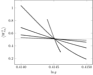
$\left\langle W_{xy}^{2}\right\rangle$-curves for the ${\mathbb{CP}^{1}}$-model are shown in Fig. 2 for system sizes $L=16,32,64,128,256$. All the curves intersect at approximately the same point, $(\ln g_{\text{c}},\left\langle W_{xy}^{2}\right\rangle)\approx(0.4145,0.511)$ – as expected from finite size scaling (FSS) for a phase transition. The phase transition is verified in Fig. 3, where the phase stiffness $\left\langle W_{xy}^{2}\right\rangle L^{-1}$ is shown to go to a finite value for a coupling less than the critical coupling $\ln g_{\text{c}}$ and to zero for a coupling greater than $\ln g_{\text{c}}$.

Figure 2: Finite size scaling for $\left\langle W_{xy}^{2}\right\rangle$-curves for the ${\mathbb{CP}^{1}}$-model. $L=16,32,64,128,256$. The horizontal line at $\left\langle W_{xy}^{2}\right\rangle=0.511$ indicates the (approximate) size independent crossing point.

Figure 3: Finite size scaling for the phase stiffness $\left\langle W_{xy}^{2}\right\rangle L^{-1}$ for the ${\mathbb{CP}^{1}}$-model, showing the behavior on each side of the critical point $\ln g_{\text{c}}\approx 0.4145$. Error bars are smaller than symbol sizes. Lines are guides to the eye.

A background field is introduced by initializing a fraction $f$ of the lattice with a nonzero current $I_{j1\tau}=1$, i.e. $f=L^{-1}\sum_{j}I_{j1\tau}$. See Fig. 1. If such a field (with $f>0$) is included in the model, the situation changes dramatically. Let $\left\langle W_{xy,f}^{2}\right\rangle$ denote $\left\langle W_{xy}^{2}\right\rangle$ in this case. Figure 5 shows $\left\langle W_{xy,f}^{2}\right\rangle$-curves for $f=1/64$ and $f=1/16$, which is to be compared with Fig. 2. The curves shift to the right as the system size is increased, with no signs of converging even for large systems; there are no size-independent crossing points.

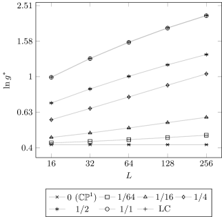
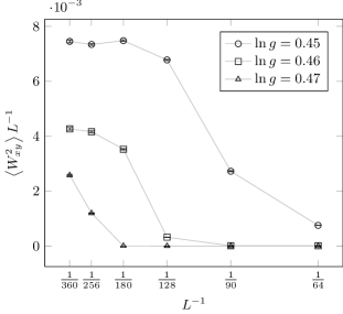
The divergence of the $\left\langle W_{xy,f}^{2}\right\rangle$-curves becomes clearer if we define a pseudocritical (finite-size critical) coupling $\ln g^{*}_{f}$ by choosing the value of $\left\langle W_{xy,f}^{2}\right\rangle(\ln g^{*}_{f})=0.511\approx\left\langle W_{xy,0}^{2}\right\rangle(\ln g_{\text{c}})$ for all $f$, and plot $\ln g^{*}_{f}$ as a function of system size. This is shown in Fig. 4 for system sizes $L=16,\ldots,256$ and several $f$-values up to 1 (maximal uniform background current field), in addition to the result for the LC model (maximally staggered background current field). It is seen from Fig. 4 that $\ln g^{*}_{f}$ increases monotonically with $L$ for all values of $f$, and more so for larger values of $f$ than for small values of $f$. The increase in $\ln g^{*}_{f}$ is clearly seen also for $f=1/64$, which is the smallest value we have considered. The range of values that $\ln g^{*}_{f}$ display in a given interval of $L$-values, increases with $f$. For $\ln g^{*}_{f}$ to take on values spanning a decade for $f=1/64$ would require enormous system sizes, beyond the capability of present-day computers. For $f=1$, the case relevant for quantum antiferromagnets on a bipartite lattice, it is seen from Fig. 4 that the range of values is much larger in the interval $L\in[16,\ldots,256]$.

Figure 4: Log-log plot of $\ln g^{*}_{f}$ as a function of system size $L$ for $f=0,\ldots,1$ as well as the LC model. The LC curve lies slightly above the $f=1$-curve. Error bars are smaller than symbol sizes. Lines are guides to the eye.

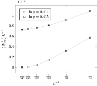
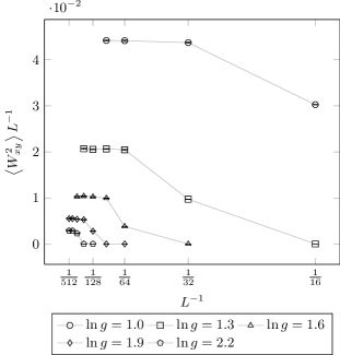
In analogy with Fig. 3, Fig. 6 shows the phase stiffness scaling for the $f=1/64$-model at three selected couplings. The stiffness always approaches a finite value for $f>0$, indicating that there is no phase transition in the thermodynamic limit. In particular, this holds for $f=1$. For this case, we have explicitly shown that the behavior is essentially the same, regardless of whether $\eta_{j}$ is staggered or not. 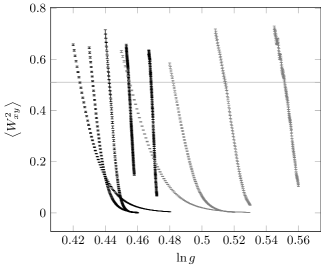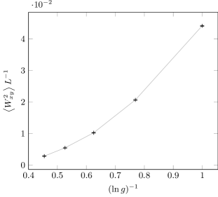Phase stiffness curves for the LC model are shown in Fig. 7, while the stiffness as a function of $(\ln g)^{-1}$ is plotted in Fig. 8. Data for larger $\ln g$ (smaller $(\ln g)^{-1}$) values are hard to obtain given the system sizes that are required, but we find it reasonable to assert, based on the extensive computations presented here, that $\left\langle W_{xy}^{2}\right\rangle L^{-1}>0$ for $(\ln g)^{-1}>0$. Note in particular how differently the curves in Fig. 7 behave from those in Fig. 3.

Figure 5: Finite size scaling for $\left\langle W_{xy,f}^{2}\right\rangle$-curves for the $f=1/64$-model (black) and the $f=1/16$-model (gray). $L=16,32,64,128,256$ for $f=1/64$ and $L=16,32,64,128$ for $f=1/16$. The horizontal line at $\left\langle W_{xy}^{2}\right\rangle=0.511$ indicates the (approximate) size independent crossing point value of the ${\mathbb{CP}^{1}}$-model ($f=0$).

Figure 6: Finite size scaling for the phase stiffness $\left\langle W_{xy,f}^{2}\right\rangle L^{-1}$ for the $f=1/64$-model at different couplings. Error bars are smaller than symbol size. Lines are guides to the eye.

Figure 7: Finite size scaling of $\left\langle W_{xy}^{2}\right\rangle L^{-1}$-curves for the LC model ($f=1$ with staggered background field) for some $\ln g$ values. $L\in\set{16,32,64,90,128,180,256,360,512}$. Lines are guides to the eye.

Figure 8: $\left\langle W_{xy}^{2}\right\rangle L^{-1}$ as a function of $(\ln g)^{-1}$ for the biggest system sizes simulated at the given $\ln g$ (which is assumed to be close to the value in the thermodynamic limit). $L=90$ for $(\ln g)^{-1}=1^{-1}=1$, $L=180$ for $(\ln g)^{-1}=1.3^{-1}\approx 0.77$, $L=256$ for $(\ln g)^{-1}=1.6^{-1}\approx 0.63$, and $L=512$ for $(\ln g)^{-1}=1.9^{-1}\approx 0.53$ and $(\ln g)^{-1}=2.2^{-1}\approx 0.45$. See Fig. 7. Lines are guides to the eye.

We conclude that for $f=0$, we obtain the phase-transition of the standard lattice ${\mathbb{CP}^{1}}$-model. In Appendix C, we show that the critical exponents we obtain are consistent with those of the $2+1$-dimensional $\mathrm{O}(3)$-model. For any nonzero value of $f$, the pseudocritical coupling appears to drift with system size, eventually appearing to diverge.

V Discussion

Finally, we briefly summarize how to understand the suppression of the phase transition in the model defined by Eq. 3. The effect originates with the Berry-phase term in the action and how it appears in the LC-model, see Eq. 9. As noted above, in the link-current representation, the effect of the Berry-phase may be viewed as the introduction of a background staggered current lattice on top of which the statistically fluctuating link-currents are imposed, Eq. 9. The ordered phase of the quantum magnet is characterized by a non-zero winding number Eq. 12.

A background current lattice of the form introduced by the Berry-phase facilitates the blow-out of closed current loops across the system at all coupling constants in the thermodynamic limit. The current lattice forms a template on which small closed current loops can connect across the system to form closed current loops with a linear extent scaling with the system size. This effectively represents a current-loop blowout, which is equivalent to ordering the original spin-system. The picture is identical to the (dual) picture of type-II superconductor in a magnetic field. At zero field, there is a genuine phase transition from an ordered to a disordered state driven by the proliferation of vortex loops. In a finite magnetic field, the situation is altered, and the field-induced vortex lattice forms a template on which small vortex-loops can connect across the system to effectively form large closed loops, thus (potentially) disordering the system.

The situation where the currents loops effectively are blown out, even at couplings where only small closed current loops would exist in a zero background current-lattice, renders the system permanently ordered, thus suppressing the phase-transition. An alternative way of viewing it more directly in the spinon-gauge field description, is that the Berry phase term suppresses instanton configurations in the compact gauge-field, equivalently suppresses hedgehog-configurations in the action. The same result obtains also in the easy-plane limit where the ${\mathbb{CP}^{1}}$-constraint $\left|z_{1}\right|^{2}+\left|z_{2}\right|^{2}=1$ is replaced by individually constant matter-field amplitudes. In that case, the instantons that are suppressed correspond to the suppression of skyrmion-antiskyrmion configurations.

Appendix A Exact link-current mapping of the model, Eq. 3.

We start out with a symmetrized form of the partition function,

$$\mathcal{Z}=\prod_{j\mu}\int_{0}^{2\uppi}\frac{\mathop{\mathrm{\mathstrut d}}\nolimits\!A_{j\mu}}{2\uppi}\prod_{ja}\int\mathop{\mathrm{\mathstrut d}}\nolimits\!z_{ja}\mathop{\mathrm{\mathstrut d}}\nolimits\!z_{ja}^{*}\\ \exp\left[(2g)^{-1}\sum_{ja\kappa}\left(z_{ja}^{*}\,\mathrm{e}^{-\mathrm{i}A_{j\kappa}}z_{j+\mu,a}+\text{c.c.}\right)+\mathrm{i}2S\sum_{j}\eta_{j}A_{j\tau}\right],$$ (14)

which is obtained from Eq. 3 by using that

$$A_{j-\mu,\mu}=-A_{j,-\mu}.$$ (15)

Writing the complex scalar fields on polar form,

$$z_{ja}=\rho_{ja}\,\mathrm{e}^{\mathrm{i}\theta_{ja}},$$ (16)

$$\int\mathop{\mathrm{\mathstrut d}}\nolimits\!z_{ja}\mathop{\mathrm{\mathstrut d}}\nolimits\!z_{ja}^{*}=\int_{0}^{2\uppi}\mathop{\mathrm{\mathstrut d}}\nolimits\!\theta_{ja}\int_{0}^{\infty}\mathop{\mathrm{\mathstrut d}}\nolimits\!\rho_{ja}\ \rho_{ja},$$ (17)

the constraint Eq. 4 reads

$${\rho_{j1}}^{2}+{\rho_{j2}}^{2}=1\quad\forall j.$$ (18)

We note that Eq. 18 describes the unit circle arc in the first quadrant of the $\rho_{j1}\rho_{j2}$-plane (since $\rho_{ja}\geq 0$). We may therefore introduce a new field $\phi\in[0,\pi/2)$, given by

$$(\rho_{j1},\rho_{j2})=(\cos\phi_{j},\sin\phi_{j}),$$ (19)

such that

$$\left.\int_{0}^{\infty}\int_{0}^{\infty}\mathop{\mathrm{\mathstrut d}}\nolimits\!\rho_{j1}\mathop{\mathrm{\mathstrut d}}\nolimits\!\rho_{j2}\ \rho_{j1}\rho_{j2}\right|_{{\rho_{j1}}^{2}+{\rho_{j2}}^{2}=1}\\ =\int_{0}^{\frac{\uppi}{2}}\mathop{\mathrm{\mathstrut d}}\nolimits\!\phi_{j}\ \cos\phi_{j}\sin\phi_{j}.$$ (20)

The partition function Eq. 14, with the constraint Eq. 4 incorporated, can therefore be written

$$\mathcal{Z}=\prod_{j\mu}\int_{0}^{2\uppi}\frac{\mathop{\mathrm{\mathstrut d}}\nolimits\!A_{j\mu}}{2\uppi}\prod_{ja}\int_{0}^{2\uppi}\mathop{\mathrm{\mathstrut d}}\nolimits\!\theta_{ja}\prod_{j}\int_{0}^{\frac{\uppi}{2}}\mathop{\mathrm{\mathstrut d}}\nolimits\!\phi_{j}\\ \cos\phi_{j}\sin\phi_{j}\exp\left(\mathcal{S}_{g}+\mathrm{i}2S\sum_{j}\eta_{j}A_{j\tau}\right),$$ (21)

where

$$\mathcal{S}_{g}=(2g)^{-1}\sum_{j\kappa}\Big{[}\cos\phi_{j}\cos\phi_{j+\kappa}\left(\,\mathrm{e}^{\mathrm{i}(\theta_{j+\kappa,1}-\theta_{j1}-A_{j\kappa})}+\text{c.c.}\right)\\ \sin\phi_{j}\sin\phi_{j+\kappa}\left(\,\mathrm{e}^{\mathrm{i}(\theta_{j+\kappa,2}-\theta_{j2}-A_{j\kappa})}+\text{c.c.}\right)\Big{]}.$$ (22)

Next, we split $\exp\mathcal{S}_{g}$ into its individual exponential factors, and Taylor expand each of them:

$$\begin{split}\exp\mathcal{S}_{g}=&\prod_{j\kappa}\sum_{\begin{subarray}{c}k_{j1\kappa}=0\\ l_{j1\kappa}=0\end{subarray}}^{\infty}\sum_{\begin{subarray}{c}k_{j2\kappa}=0\\ l_{j2\kappa}=0\end{subarray}}^{\infty}\\ \Bigg{[}&\frac{\left((2g)^{-1}\cos\phi_{j}\cos\phi_{j+\kappa}\right)^{k_{j1\kappa}+l_{j1\kappa}}}{k_{j1\kappa}!l_{j1\kappa}!}\\ &\frac{\left((2g)^{-1}\sin\phi_{j}\sin\phi_{j+\kappa}\right)^{k_{j2\kappa}+l_{j2\kappa}}}{k_{j2\kappa}!l_{j2\kappa}!}\\ &\,\mathrm{e}^{\mathrm{i}(k_{j1\kappa}-l_{j1\kappa})\left(\theta_{j+\kappa,1}-\theta_{j1}-A_{j\kappa}\right)}\\ &\,\mathrm{e}^{\mathrm{i}(k_{j2\kappa}-l_{j2\kappa})\left(\theta_{j+\kappa,2}-\theta_{j2}-A_{j\kappa}\right)}\Bigg{]}.\end{split}$$ (23)

Here $k_{ja\kappa}$ and $l_{ja\kappa}$ may be seen as Taylor expansion index fields.

Inserting Eq. 23 into Eq. 21 and rearranging (and relabelling) the terms, the partition function reads

$$\begin{split}\mathcal{Z}=&\sum_{\set{k,l}}\prod_{j\mu}\int_{0}^{2\uppi}\frac{\mathop{\mathrm{\mathstrut d}}\nolimits\!A_{j\mu}}{2\uppi}\prod_{ja}\int_{0}^{2\uppi}\mathop{\mathrm{\mathstrut d}}\nolimits\!\theta_{ja}\prod_{j}\int_{0}^{\frac{\uppi}{2}}\mathop{\mathrm{\mathstrut d}}\nolimits\!\phi_{j}\\ &\prod_{ja\kappa}\,\mathrm{e}^{\mathrm{i}\theta_{ja}\left(k_{ja\kappa}-l_{ja\kappa}-k_{j+\kappa,a,-\kappa}+l_{j+\kappa,a,-\kappa}\right)}\\ &\prod_{j}\,\mathrm{e}^{\mathrm{i}2S\eta_{j}A_{j\tau}}\prod_{ja\kappa}\,\mathrm{e}^{\mathrm{i}(k_{ja\kappa}-l_{ja\kappa})A_{j\kappa}}\\ &\prod_{j\kappa}\cos^{(k_{j1\kappa}+l_{j1\kappa}+k_{j+\kappa,1,-\kappa}+l_{j+\kappa,1,-\kappa})+1}\phi_{j}\\ &\prod_{j\kappa}\sin^{(k_{j2\kappa}+l_{j2\kappa}+k_{j+\kappa,2,-\kappa}+l_{j+\kappa,2,-\kappa})+1}\phi_{j}\\ &\prod_{ja\kappa}\frac{(2g)^{-(k_{ja\kappa}+l_{ja\kappa})}}{k_{ja\kappa}!l_{ja\kappa}!}.\end{split}$$ (24)

$\set{k,l}$ denotes the set of all possible Taylor expansion index field configurations.

It is convenient to introduce (what will turn out to be) the non-negative bond subcurrents

$$J_{ja\kappa}\equiv k_{ja\kappa}+l_{j+\kappa,a,-\kappa}\in\mathbb{N}_{0},$$ (25)

as well as the total bond currents

$$\quad I_{ja\kappa}\equiv J_{ja\kappa}-J_{j+\kappa,a,-\kappa}\in\mathbb{Z},$$ (26)

and the factor

$$\mathcal{N}_{ja} \equiv\frac{1}{2}\sum_{\kappa}k_{ja\kappa}+l_{ja\kappa}+k_{j+\kappa,a,-\kappa}+l_{j+\kappa,a,-\kappa}$$

$$=\frac{1}{2}\sum_{\kappa}J_{ja\kappa}+J_{j+\kappa,a,-\kappa}.$$ (27)

Using these definitions, as well as Eq. 15 and some more rearranging of terms, the partition function, Eq. 24, can be written on the form

$$\begin{split}\mathcal{Z}=&\sum_{\set{k,l}}\prod_{j\mu}\int_{0}^{2\uppi}\frac{\mathop{\mathrm{\mathstrut d}}\nolimits\!A_{j\mu}}{2\uppi}\prod_{ja}\int_{0}^{2\uppi}\mathop{\mathrm{\mathstrut d}}\nolimits\!\theta_{ja}\prod_{j}\int_{0}^{\frac{\uppi}{2}}\mathop{\mathrm{\mathstrut d}}\nolimits\!\phi_{j}\\ &\prod_{ja}\,\mathrm{e}^{\mathrm{i}\theta_{ja}\sum_{\kappa}I_{ja\kappa}}\\ &\prod_{j}\,\mathrm{e}^{\mathrm{i}\left(2S\eta_{j}A_{j\tau}+\sum_{\mu}(I_{j1\mu}+I_{j2\mu})A_{j\mu}\right)}\\ &\prod_{j}\cos^{2\mathcal{N}_{j1}+1}\phi_{j}\sin^{2\mathcal{N}_{j2}+1}\phi_{j}\\ &\prod_{ja\kappa}\frac{(2g)^{-J_{ja\kappa}}}{k_{ja\kappa}!l_{ja\kappa}!}.\end{split}$$ (28)

Note that the summation goes over positive directions only in the gauge field factor.

The partition function is now on a form where the integrals are decoupled and may be performed easily.

The integration of the $\theta$-field in Eq. 28 gives just a Kronecker delta (up to an irrelevant scaling factor) at each lattice site. Hence, we obtain the total bond-current conservation constraint, or “Kirchhoff’s law”,

$$\sum_{\kappa}I_{ja\kappa}=0,\quad\forall j,a.$$ (29)

Note also that this, by the definition Eq. 26, implies that Eq. 27 may be simplified to

$$\mathcal{N}_{ja}=\sum_{\kappa}J_{ja\kappa}\in\mathcal{N}_{0}.$$ (30)

In the same way as for the $\theta$-integration, the gauge-field integration gives Kronecker deltas, leading to the coupling of the components,

$$\begin{gathered}I_{j1x}+I_{j2x}=0,\\ I_{j1y}+I_{j2y}=0,\\ I_{j1\tau}+I_{j2\tau}+2S\eta_{j}=0.\end{gathered}$$ (31)

The $\phi$-field is integrated out by

$$\int_{0}^{\frac{\uppi}{2}}\mathop{\mathrm{\mathstrut d}}\nolimits\!\phi_{j}\cos^{2\mathcal{N}_{j1}+1}\phi_{j}\sin^{2\mathcal{N}_{j2}+1}\phi_{j}\\ =\frac{\mathcal{N}_{j1}!\mathcal{N}_{j2}!}{2\left(\mathcal{N}_{j1}+\mathcal{N}_{j2}+1\right)!},$$ (32)

where we have used the identity

$$\int_{0}^{\frac{\uppi}{2}}\cos^{m}x\sin^{n}x\mathop{\mathrm{\mathstrut d}}\nolimits\!x\\ =\frac{\Gamma\left(\frac{m+1}{2}\right)\Gamma\left(\frac{n+1}{2}\right)}{2\Gamma\left(\frac{m+n+2}{2}\right)},\quad m,n>0.$$ (33)

We will ignore the physically irrelevant multiplicative factor of $2$ in the denominator of Eq. 32 in the final expression for the partition function.

The last factor we have to deal with is

$$\sum_{\set{k,l}}\prod_{ja\kappa}\frac{(2g)^{-J_{ja\kappa}}}{k_{ja\kappa}!l_{ja\kappa}!}.$$ (34)

We have included the sum over all possible $k,l$ field configurations, as we want to change Eq. 34 to a sum over all possible $J$-current field configurations, $\set{J}$, instead. (There is no problem with this, as all the other terms in the partition function and the constraints are – as we have seen – exclusively $J$ dependent.) Using the definition of the positive bond currents, Eq. 25, as well as some standard combinatorial results, we may rewrite Eq. 34 as

$$\sum_{\set{k,l}}\prod_{ja\kappa}\frac{(2g)^{-J_{ja\kappa}}}{k_{ja\kappa}!l_{ja\kappa}!} =\sum_{\set{J}}\prod_{ja\kappa}\sum_{k_{ja\kappa}=0}^{J_{ja\kappa}}\frac{(2g)^{-J_{ja\kappa}}}{k_{ja\kappa}!(J_{ja\kappa}-k_{ja\kappa})!}$$

$$=\sum_{\set{J}}\prod_{ja\kappa}\frac{(2g)^{-J_{ja\kappa}}}{J_{ja\kappa}!}\sum_{k_{ja\kappa}=0}^{J_{ja\kappa}}\binom{J_{ja\kappa}}{k_{ja\kappa}}$$

$$=\sum_{\set{J}}\prod_{ja\kappa}\frac{(2g)^{-J_{ja\kappa}}}{J_{ja\kappa}!}2^{J_{ja\kappa}}$$

$$=\sum_{\set{J}}\prod_{ja\kappa}\frac{g^{-J_{ja\kappa}}}{J_{ja\kappa}!}$$ (35)

Collecting all of the above gives the desired results Eqs. 5, 6, 7, 8 and 9.

Appendix B Link-current representation of the model with basic representation of the Berry-phase

The basic form of the Berry-phase contribution to the action is given by Read and Sachdev (1990)

$$\mathcal{S}_{\text{B}}=2S\sum_{ia}\eta_{i}\int_{0}^{\beta}z_{a}^{*}(\boldsymbol{\mathbf{r}}_{i},\tau)\frac{\mathop{\mathrm{\mathstrut d}}\nolimits\!z_{a}(\boldsymbol{\mathbf{r}}_{i},\tau)}{\mathop{\mathrm{\mathstrut d}}\nolimits\!\tau}\mathop{\mathrm{\mathstrut d}}\nolimits\!\tau,$$ (36)

which, when discretizing imaginary time and ignoring irrelevant constants, may be written

$$\begin{split}\mathcal{S}_{\text{B}}&=2S\sum_{ja}\eta_{j}z_{ja\tau}^{*}z_{j+\tau,a\tau}\\ &=2S\sum_{j}\eta_{j}\Bigl{(}\cos\phi_{j}\cos\phi_{j+\tau}\,\mathrm{e}^{\mathrm{i}(\theta_{j+\tau,1}-\theta_{j1})}\\ &\hphantom{{}=2S\sum_{j}\eta_{j}\Bigl{(}}+\sin\phi_{j}\sin\phi_{j+\tau}\,\mathrm{e}^{\mathrm{i}(\theta_{j+\tau,2}-\theta_{j2})}\Bigr{)},\end{split}$$ (37)

in the $\beta\to\infty$ limit. We have introduced the fields $\theta$ and $\phi$ defined in Eqs. 16 and 19. Note that Eq. 37 may not be symmetrized.

Replacing the Berry-phase term of partition function (21), $\mathrm{i}2S\sum_{j}\eta_{j}A_{j\tau}$, with Eq. 37, the link-current mapping may proceed in the same way as in Appendix A. The details of how to approximate the form of the Berry phase given in Eq. 37 to the form of the Berry phase given in Eq. 3, is provided in Chapter 13 of Ref. Sachdev, 1999.

Taylor expanding $\exp\mathcal{S}_{\text{B}}$ gives an additional expansion index field $m_{ja}\in\mathbb{N}_{0}$ coupling in the $\tau$ direction, so the partition function equivalent to Eq. 28 reads

$$\begin{split}\mathcal{Z}=&\sum_{\set{k,l,m}}\prod_{j\mu}\int_{0}^{2\uppi}\frac{\mathop{\mathrm{\mathstrut d}}\nolimits\!A_{j\mu}}{2\uppi}\prod_{ja}\int_{0}^{2\uppi}\mathop{\mathrm{\mathstrut d}}\nolimits\!\theta_{ja}\prod_{j}\int_{0}^{\frac{\uppi}{2}}\mathop{\mathrm{\mathstrut d}}\nolimits\!\phi_{j}\\ &\prod_{ja}\,\mathrm{e}^{\mathrm{i}\theta_{ja}\left(m_{j-\tau,a}-m_{j,a}+\sum_{\kappa}I_{ja\kappa}\right)}\\ &\prod_{j}\,\mathrm{e}^{\mathrm{i}\sum_{\mu}(I_{j1\mu}+I_{j2\mu})A_{j\mu}}\\ &\prod_{j}\cos^{2\mathcal{N}_{j1}+1+m_{j1}+m_{j-\tau,1}}\phi_{j}\sin^{2\mathcal{N}_{j2}+1+m_{j2}+m_{j-\tau,2}}\phi_{j}\\ &\prod_{ja\kappa}\frac{(2g)^{-J_{ja\kappa}}}{k_{ja\kappa}!l_{ja\kappa}!}\prod_{ja}\frac{(2S\eta_{j})^{m_{ja}}}{m_{ja}!}.\end{split}$$ (38)

The field integrals can be done as before, leading to the new constraints

$$m_{j-\tau,a}-m_{j,a}+\sum_{\kappa}I_{ja\kappa}=0,$$ (39)

$$I_{j1\mu}+I_{j2\mu}=0.$$ (40)

Using Eq. 35 (which is independent of the $m$-field, and thus still valid) and Eq. 33, we are left with the partition function

$$\mathcal{Z}=\sum_{\set{J,m}}\prod_{ja}\frac{(2S\eta_{j})^{m_{ja}}}{m_{ja}!}\prod_{ja\kappa}\frac{g^{-J_{ja\kappa}}}{J_{ja\kappa}!}\\ \prod_{j}\frac{\prod_{a}\Gamma\left(\mathcal{N}_{ja}+1+\frac{1}{2}(m_{ja}+m_{j-\tau,a})\right)}{\Gamma\left(\sum_{a}\mathcal{N}_{ja}+1+\frac{1}{2}(m_{ja}+m_{j-\tau,a})\right)},$$ (41)

which should be compared to Eq. 5. The main problem with this formulation is that a sign problem arises from the factors $\eta_{j}^{m_{ja}}=\pm 1$, rendering the model hard to deal with in Monte Carlo simulations.

Appendix C Critical exponents for the ${\mathbb{CP}^{1}}$-model

If we define the global magnetization $\boldsymbol{\mathbf{m}}\equiv N^{-1}\sum_{j}\boldsymbol{\mathbf{n}}_{j},\quad N\equiv L^{3}$, and use the definition of $\boldsymbol{\mathbf{n}}_{j}$ in terms of Pauli matrices and the $z$-fields, Eq. 1, we end up with the relation

$$\left\langle m_{x}^{2}+m_{y}^{2}\right\rangle=\frac{2}{N}\sum_{j}h(j),$$ (42)

where

$$h(i-j)\equiv\left\langle z_{i1}z_{j1}^{*}z_{i2}^{*}z_{j2}+\text{c.c.}\right\rangle.$$ (43)

Now, for the ${\mathbb{CP}^{1}}$-model, we have

$$\left\langle z_{i^{\prime}1}z_{j^{\prime}1}^{*}z_{i^{\prime}2}^{*}z_{j^{\prime}2}\right\rangle=\mathcal{Z}_{{\mathbb{CP}^{1}}}^{-1}\mathcal{W}_{i^{\prime}j^{\prime}},$$ (44)

where

$$\mathcal{W}_{i^{\prime}j^{\prime}}=\prod_{j\mu}\int_{0}^{2\uppi}\frac{\mathop{\mathrm{\mathstrut d}}\nolimits\!A_{j\mu}}{2\uppi}\prod_{ja}\int\mathop{\mathrm{\mathstrut d}}\nolimits\!z_{ja}\mathop{\mathrm{\mathstrut d}}\nolimits\!z_{ja}^{*}z_{i^{\prime}1}z_{j^{\prime}1}^{*}z_{i^{\prime}2}^{*}z_{j^{\prime}2}\\ \exp\left[g^{-1}\sum_{ja\mu}\left(z_{ja}^{*}\,\mathrm{e}^{-\mathrm{i}A_{j\mu}}z_{j+\mu,a}+\text{c.c.}\right)\right],$$ (45)

with the usual ${\mathbb{CP}^{1}}$-constraint Eq. 4. In the link-current formalism, Eq. 45 becomes (using the procedures of Appendix A)

$$\mathcal{W}_{i^{\prime}j^{\prime}}=\sum_{\set{J}}\prod_{ja\kappa}\frac{g^{-J_{ja\kappa}}}{J_{ja\kappa}!}\prod_{j\neq i^{\prime},j^{\prime}}\left[\frac{\mathcal{N}_{j1}!\mathcal{N}_{j2}!}{\left(\mathcal{N}_{j1}+\mathcal{N}_{j2}+1\right)!}\right]Q_{i^{\prime}j^{\prime}},$$ (46)

$$Q_{i^{\prime}j^{\prime}}=\left\{\begin{aligned} &\frac{\left(\mathcal{N}_{i^{\prime}1}+1\right)!\left(\mathcal{N}_{i^{\prime}2}+1\right)!}{\left(\mathcal{N}_{i^{\prime}1}+\mathcal{N}_{i^{\prime}2}+3\right)!},\quad i^{\prime}=j^{\prime}\\ &\frac{\prod_{a}\Gamma\left(\mathcal{N}_{i^{\prime}a}+\frac{3}{2}\right)\Gamma\left(\mathcal{N}_{j^{\prime}a}+\frac{3}{2}\right)}{\left(\mathcal{N}_{i^{\prime}1}+\mathcal{N}_{i^{\prime}2}+2\right)!\left(\mathcal{N}_{j^{\prime}1}+\mathcal{N}_{j^{\prime}2}+2\right)!},\quad i^{\prime}\neq j^{\prime},\end{aligned}\right.$$ (47)

with the constraints

$$I_{j1\mu}+I_{j2\mu}=0,$$ (48)

$$\sum_{\kappa}I_{j1\kappa}=\left\{\begin{aligned} -1,&\quad j=i^{\prime}\\ 1,&\quad j=j^{\prime}\\ 0,&\quad j\neq i^{\prime},j^{\prime}\end{aligned}\right.$$ (49)

We get $\mathcal{W}_{i^{\prime},j^{\prime}}^{*}$ by interchanging $i^{\prime}\leftrightarrow j^{\prime}$ in the last constraint.

Equation 49 means that $h(i-j)$ must be sampled for a field configuration where all current loops/worms but one are closed. The open worm has its head(tail) at lattice site $i$ and tail(head) at $j$. Since the worm is already following the probability distribution given by the partition function $\mathcal{Z}_{{\mathbb{CP}^{1}}}$, the weight associated with this “background” distribution must be divided out before we can sample $h$ properly. Hence, to sample $\left\langle m_{xy}^{2}\right\rangle\equiv\left\langle m_{x}^{2}+m_{y}^{2}\right\rangle/2$, we store

$$M^{2}\leftarrow M^{2}+\left\{\begin{aligned} &\frac{\left(\mathcal{N}_{i1}+1\right)\left(\mathcal{N}_{i2}+1\right)}{\left(\mathcal{N}_{i1}+\mathcal{N}_{i2}+2\right)\left(\mathcal{N}_{i1}+\mathcal{N}_{i2}+3\right)},\quad i-j=0\\ &\frac{1}{\left(\mathcal{N}_{i1}+\mathcal{N}_{i2}+2\right)\left(\mathcal{N}_{j1}+\mathcal{N}_{j2}+2\right)}\\ &\times\prod_{a}\frac{\Gamma\left(\mathcal{N}_{ia}+\frac{3}{2}\right)\Gamma\left(\mathcal{N}_{ja}+\frac{3}{2}\right)}{\mathcal{N}_{ia}!\mathcal{N}_{ja}!},\quad i-j\neq 0\end{aligned}\right.$$ (50)

at each Monte Carlo step, along with

$$Z\leftarrow Z+1$$ (51)

each time the worm closes ($i=j$). The unbiased Monte Carlo estimator $\left\langle m_{xy}^{2}\right\rangle_{\text{MC}}$ is then given by

$$\left\langle m_{xy}^{2}\right\rangle_{\text{MC}}=\frac{M^{2}}{NZ}$$ (52)

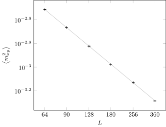
From FSS, we expect $\left\langle m_{xy}^{2}\right\rangle\sim L^{-\frac{2\beta}{\nu}}$ at criticality. We find $\beta/\nu=$0.513(4)$$ in an FSS analysis for system sizes up to $L=360$, see Fig. 9. This is in reasonable agreement with the $\mathrm{O}(3)$ universality class result of Ref. Campostrini et al., 2002, $\beta/\nu=$0.5187(6)$$.

Figure 9: log-log plot of the finite size scaling of $\left\langle m_{xy}^{2}\right\rangle$ for the ${\mathbb{CP}^{1}}$-model at $\ln g=$0.414\,504$\approx\ln g_{\text{c}}$ (markers), plotted together with a scaling curve $\sim L^{-2\times 0.513}$ (light gray).