Indications of a sub-linear and non-universal Kennicutt-Schmidt relationship

Abstract

We estimate the parameters of the Kennicutt-Schmidt (KS) relationship, linking the star formation rate ($\Sigma_{\rm SFR}$) to the molecular gas surface density ($\Sigma_{\rm mol}$), in the STING sample of nearby disk galaxies using a hierarchical Bayesian method. This method rigorously treats measurement uncertainties, and provides accurate parameter estimates for both individual galaxies and the entire population. Assuming standard conversion factors to estimate $\Sigma_{\rm SFR}$ and $\Sigma_{\rm mol}$ from the observations, we find that the KS parameters vary between galaxies, indicating that no universal relationship holds for all galaxies. The KS slope of the whole population is 0.76, with the $2\sigma$ range extending from 0.58 to 0.94. These results imply that the molecular gas depletion time is not constant, but varies from galaxy to galaxy, and increases with the molecular gas surface density. Therefore, other galactic properties besides just $\Sigma_{\rm mol}$ affect $\Sigma_{\rm SFR}$, such as the gas fraction or stellar mass. The non-universality of the KS relationship indicates that a comprehensive theory of star formation must take into account additional physical processes that may vary from galaxy to galaxy.

1 Introduction

As stars form in molecular gas, quantifying the relationship between the star formation rate $\Sigma_{\rm SFR}$ and molecular gas surface density $\Sigma_{\rm mol}$ is a prerequisite for understanding star formation in the interstellar medium (ISM). Most observational studies indicate a power-law dependency

$$\Sigma_{\rm SFR}=a\Sigma_{\rm mol}^{N},$$ (1)

which is often called the “Kennicutt-Schmidt” (KS) relationship (Schmidt, 1959; Kennicutt, 1989). The slope $N$ is a critical parameter of various proposed theories of star formation (see e.g. Mac Low & Klessen, 2004; McKee & Ostriker, 2007; Kennicutt & Evans, 2012, and references therein). Consequently, over the last few decades, many observational investigations have focused on estimating the parameters $a$ and $N$ (e.g. Kennicutt, 1989, 1998; Rownd & Young, 1999; Wong & Blitz, 2002; Kennicutt et al., 2007; Bigiel et al., 2008, 2011; Leroy et al., 2008; Schruba et al., 2011).

The index $N$, often referred to as the KS slope, provides information about the molecular gas depletion time $\tau_{\rm dep}^{\rm CO}$, or its inverse, the star formation efficiency over a free-fall time. The first systematic extra-galactic studies by Kennicutt (1989, 1998) estimated $N$$\sim$1.5, considering both atomic and molecular gas, suggesting that the depletion time (efficiency) decreases (increases) with higher total gas densities. More recently, analyses of resolved observations in the HERACLES (Leroy et al., 2009) and STING (Rahman et al., 2012, hereafter R12) samples have proposed a linear KS relationship (i.e. $N$=1) for the population, often interpreted as a consequence of constant gas depletion times (efficiency), with $\tau_{\rm dep}^{\rm CO}$$\sim$2 Gyr. These and other studies also clearly demonstrate, however, that the large scatter in the observed trends is indicative that a single KS relationship cannot fully describe the $\Sigma_{\rm SFR}$- $\Sigma_{\rm mol}$ relationship (Bigiel et al., 2008; Schruba et al., 2011; Saintonge et al., 2011; Leroy et al., 2013, R12). Shetty et al. (2013), hereafter SKB13, by performing an analysis on seven of the HERACLES galaxies using robust Bayesian statistical methods, reaffirm that the KS index is not constant from galaxy-to-galaxy, but in addition find that a sub-linear relationship better describes the data for some individual galaxies such as M51. This suggests, therefore, that $\tau_{\rm dep}^{\rm CO}$ increases at higher $\Sigma_{\rm mol}$ for these galaxies.

In SKB13, we demonstrated that hierarchical statistical modeling provides significantly more accurate parameter estimates than traditional least-squares fitting methods, which is often applied non-hierarchically to data from all galaxies. Moreover, Bayesian methods allow for a rigorous treatment of measurement uncertainties (Gelman et al., 2004; Kelly, 2007; Kruschke, 2011). One question that emerges from the SKB13 analysis is whether other observational efforts that infer a linear or super-linear KS relationship are simply a consequence of the chosen statistical method, or an intrinsic relationship accurately manifested by the data.

In this work, we employ the hierarchical Bayesian method described in SKB13 to estimate the KS parameters from the STING observational survey (Rahman et al., 2011, hereafter R11, and R12). Compared to the Bigiel et al. (2008) HERACLES sub-sample, the STING sample contains nearly twice as many galaxies (13 compared to 7). In the next section we briefly describe the STING survey. In Section 3 we review the hierarchical Bayesian fitting method. Section 4 presents the results of the fit on the STING data. After a discussion in Section 5, we conclude with a summary in Section 6.

2 Observations

We estimate the parameters of the KS relationship using the observational data from the Survey Toward Infrared-Bright Nearby Galaxies (STING; R11, R12). Following SKB13 we denote ${\hat{\Sigma}_{\rm SFR}}$ or ${\hat{\Sigma}_{\rm mol}}$ as the measured values, and $\Sigma_{\rm SFR}$ or $\Sigma_{\rm mol}$ as the true values of the relevant parameters. The STING dataset contains CARMA CO ($J=1-0$) observations of nearby disk galaxies, which indirectly provide estimates of ${\hat{\Sigma}_{\rm mol}}$. The (FWHM) resolution varies from 3″ to 5″. The Spitzer (MIPS) 24 µm images of these galaxies provides estimates of ${\hat{\Sigma}_{\rm SFR}}$, which have $\sim$6″ resolution. As described in R11, we use the Nyquist sampled maps regrided to the same 1 kpc pixel scale. Though the MIPS point spread function (PSF) is not a simple Gaussian, for many of the galaxies the native resolution corresponds to substantially less than 1 kpc. The appropriate convolution thereby minimizes the influence of the non-Gaussian features of the PSF. Further, we have investigated how a more accurate convolution kernel (Aniano et al., 2011) could affect our results. Though the KS slopes for some galaxies increase by $\sim$0.1-0.3, the conclusions reported in the next section are not significantly affected. In our study, as in R12, we only consider regions where $\Sigma_{\rm mol}$ $\geq$ 20 M_⊙ pc^-2, where the signal to noise is high. For these data, the relative uncertainties of the measured CO intensities range from $\sim 10-20\%$.

The first two columns of Table 1 lists the galaxies and the number of measurements in the STING sample. We refer the reader to R11 and R12 for a more thorough description of the observations and data reduction.

3 Modelling Method

The hierarchical Bayesian method we employ here is described in SKB13, where we also demonstrated its accuracy and advantage over traditional least squares methods, such as the bisector. Here we only provide a brief description, and refer to SKB13 for the details of the method.

Our goal is to estimate the KS parameters of each individual galaxy, as well as the mean value of the population (group). Fitting a single model to combined data may conceal intrinsic variations between individuals (see also Gelman & Hill, 2007). Assessing the KS parameters from observations of many regions (or beams) within a number of galaxies is precisely a problem for which hierarchical methods can provide robust solutions.

Furthermore, hierarchical Bayesian methods allow for a rigorous treatment of measurement uncertainties. For example, the ${\hat{\Sigma}_{\rm SFR}}$ and ${\hat{\Sigma}_{\rm mol}}$ may not be accurate due to noise and possible errors in the assumed conversion factors. By performing Markov Chain Monte Carlo simulations (MCMC), the analysis explores the true value of $\Sigma_{\rm SFR}$ and $\Sigma_{\rm mol}$ given the measurement ${\hat{\Sigma}_{\rm SFR}}$ and ${\hat{\Sigma}_{\rm mol}}$ and their uncertainties.

After a large number of MCMC steps, the outcome of the Bayesian analysis, or the posterior, is a probability distribution function (PDF) for each unknown parameter, including those defining the KS relationship. Therefore, the posterior provides PDFs of plausible values for the parameters, thoroughly accounting for the uncertainties in the measurements or any other quantity, such as the conversion factors, required in the modelling.

4 Results

4.1 The KS relationship of the STING galaxies

The quantities ${\hat{\Sigma}_{\rm SFR}}$ and ${\hat{\Sigma}_{\rm mol}}$ are not measured directly. Instead, we follow the conventional practice and infer these quantities from CO and IR observations using fixed conversion factors. The $X_{\rm CO}$ factor directly provides ${\hat{\Sigma}_{\rm mol}}$ from the CO observations, and we use the standard Galactic value, $X_{\rm CO}$ = $2\times 10^{20}$ cm^-2 K^-1 km^-1 s, converted to M_⊙ pc^-2 units, including a factor of 1.4 to account for the contribution from He (see Bolatto et al., 2013, and references therein). We have confirmed that allowing $X_{\rm CO}$ to vary freely within a suitable range (e.g. Shetty et al., 2011a, b) does not change our results. To compute the star formation rate from the 24 µm fluxes, we utilize the conversion factor described by Calzetti et al. (2007): SFR(M_⊙ yr^-1) = 1.27$\times 10^{−38}[\nu$L₂₄(erg s⁻¹)]^0.8850.

The model requires suitable estimates of the uncertainties. As the largest sources of error are likely the conversion factors, we choose uncertainties of 25% and 50% for ${\hat{\Sigma}_{\rm mol}}$ and ${\hat{\Sigma}_{\rm SFR}}$, respectively. These are possibly larger than the true uncertainties, but we prefer to be conservative in our error estimates.

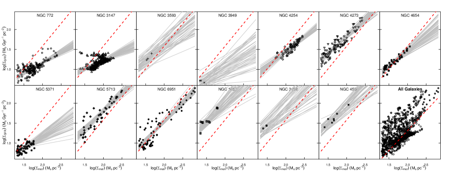
Figure 1: Star formation rates and surface densities of 13 STING galaxies. Black symbols show the data, and gray lines show 50 random draws from the posterior. For reference, (red) dashed lines shows the bisector fit with $N$=1.1 to all data (shown together in last panel).

Figure 1 shows ${\hat{\Sigma}_{\rm SFR}}$ and ${\hat{\Sigma}_{\rm mol}}$ for thirteen galaxies, as well as the ensemble in the last panel. The gray lines are fifty random draws from the posterior, depicting representative results of the hierarchical Bayesian fit. For comparison, the red dashed line is the (non-hierarchical) bisector result $N=1.1$ on all datapoints (shown in the last panel). Clearly, for many galaxies the linear bisector result cannot reproduce the $\Sigma_{\rm SFR}$ - $\Sigma_{\rm mol}$ trend. For the galaxies with the largest deviations from the bisector, such as NGC 772, NGC 3147, and NGC 4254, the data strongly evinces a sub-linear KS relationship.

Table 1 shows the Bayesian parameter estimates of the KS relationship (with $A=\log a$) for all individuals and the population. Columns 3 - 7 present the KS parameter estimates for each individual galaxy, including the $2\sigma$ extent and the scatter $\sigma_{\rm scat}$ about the regression. The last row indicates the parameter estimates for the population. For five of the thirteen galaxies, the data is inconsistent with a linear KS relationship at the $2\sigma$ level. Further, the mean slope of the ensemble is estimated to be between 0.58 and 0.94, favoring a sub-linear KS relationship with 95% confidence. Similar to the results from SKB13, there is significant galaxy-to-galaxy variation, indicating that no single KS relationship provides an accurate fit for all galaxies.

Since the posterior contains PDFs for the unknown parameters for each individual, we can take differences in $N$ to ascertain whether the galaxies have similar KS relationships. For NGC 0772 and NGC 4273, for instance, this PDF contains no values close to zero, revealing that these galaxies have different KS relationships.

We can also estimate, generically, how many galaxies would have sub-linear KS slopes. Though we have find that five individual galaxies from the STING sample have sub-linear slopes at 95% confidence, the total number of galaxies with sub-linear slopes predicted by the posterior may different. At the end of the MCMC analysis, we can evaluate the PDF of the number of galaxies with sub-linear slopes. The Bayesian results indicate that at 95% confidence at least 9 galaxies will have sub-linear KS relationships.

4.2 The molecular gas depletion time of STING galaxies

The gas depletion time is defined as

$$\tau_{\rm dep}^{\rm CO}=\Sigma_{\rm mol}/\Sigma_{\rm SFR},$$ (2)

where we include “CO” in the superscript to emphasize that $\tau_{\rm dep}^{\rm CO}$ corresponds to the depletion time of the gas traced by CO.

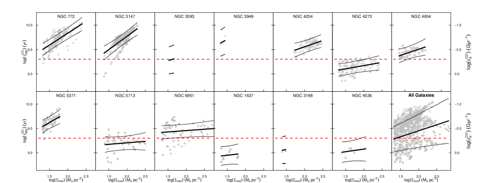
Figure 2: Depletion time $\tau_{\rm dep}^{\rm CO}$ and surface density of STING Galaxies. Points indicate the directly measured values. Solid line is the median of the Bayesian estimate, and thin lines mark the $2\sigma$ interval. The red dashed line indicates $\tau_{\rm dep}^{\rm CO}$=2 Gyr. The efficiency per free fall time ($\epsilon_{\rm ff}^{CO}$) is marked on the right ordinate.

Figure 2 shows $\tau_{\rm dep}^{\rm CO}$ using the measured values of ${\hat{\Sigma}_{\rm SFR}}$ and ${\hat{\Sigma}_{\rm mol}}$ in Equation 2 directly, as well as the Bayesian fit with the $2\sigma$ uncertainty range. The Bayesian model predictions for each galaxy at four values of $\Sigma_{\rm mol}$=50, 100, 150, and 200 M_⊙ pc^-2 are provided in Table 1.

As with the KS relationship itself in Figure 1, there is no single $\tau_{\rm dep}^{\rm CO}$ that holds for all galaxies. Further, for those galaxies with a strongly sub-linear relationship, $\tau_{\rm dep}^{\rm CO}$ clearly increases with increasing gas surface density.

For instance, for NGC 772 where the median $N$=0.51, the median $\tau_{\rm dep}^{\rm CO}$ varies from  $\buildrel<\over{\sim}$ 5 Gyr at $\Sigma_{\rm mol}$=50 M_⊙ pc^-2, to  $\buildrel>\over{\sim}$ 9 Gyr at $\Sigma_{\rm mol}$=200 M_⊙ pc^-2. Altogether, a constant value of $\tau_{\rm dep}^{\rm CO}$=2 Gyr can be ruled out at 95% for all $\Sigma_{\rm mol}$$\geq$ 50 M_⊙ pc^-2 for this galaxy. Note that some galaxies are consistent with a constant depletion time. NGC 5713, for example, has $\tau_{\rm dep}^{\rm CO}$$\approx$2$\pm$1 Gyr.

5 Caveats

There are a number of caveats and assumptions that enter our analysis. Missing flux intrinsic to interferometric observations, uncertainties other than random uncorrelated errors, and variable conversion factors are all likely to affect any parameter estimates.

As noted by R11, large scale diffuse emission may not be detected by interferometers. Single-dish observations are needed for recovering this component (e.g. Helfer et al., 2003). This diffuse emission will certainly have an impact on any estimated KS relationship, as it will tend to increase the flux more in the low density regime, steepening the estimated slope. For the one galaxy for which we do have single dish data, NGC 4254, the impact of correcting for missing flux results in a slope increase of less than 0.1. Fully accounting for large scale emission may therefore impact the KS parameter estimates. In our analysis we have attempted to minimize the effect of diffuse emission by only considering CO bright regions (with $\Sigma_{\rm mol}$ $\geq$ 20 M_⊙ pc^-2). In principle, for completeness single-dish observations would be required.

In the hierarchical modelling, we have only considered random statistical uncertainties. However, we have been very conservative and have adopted rather “wide” priors. They are larger than the noise estimates for the CO and IR fluxes. This implicitly accounts for unknown sources of errors. For example, there are gain and noise uncertainties, which we have not treated separately. As these errors are probably uncorrelated, using a single prior for the overall uncertainty likely does not unduly affect the results. However, two possible sources of correlated uncertainties are the conversion factors from the observed intensities to $\Sigma_{\rm SFR}$ and $\Sigma_{\rm mol}$. In our analysis, if (some fraction of) the uncertainties are assigned to the conversion factors, then they are uncorrelated. However, as discussed in SKB13 these factors may correlated, and in principle hierarchical models are very well suited for investigating such correlations. We note that we have explored the possibility of correlations between the $X_{\rm CO}$ and the conversion between 24 µm and $\Sigma_{\rm SFR}$, but the current STING dataset does not provide any strong statistical evidence favoring correlated conversion factors. Future efforts with larger datasets and a more detailed treatment of individual contributions to the overall uncertainties may further reveal such correlations and their impact on the KS relationship.

Finally, we stress again that we have followed conventional practice and employed standard conversion factors. As such we are essentially modelling the correlations between the CO and 24 µm intensities. Note that though we have employed a non-linear relationship between $\Sigma_{\rm SFR}$ and the 24 µm intensities, the KS slope estimates are only marginally affected (by $\sim 0.1$) when we employ a linear conversion. Our analysis of the STING dataset indicates that to 95%, the the mean KS index of the ensemble is consistent with a sub-linear KS relationship when assuming commonly-used conversion factors, with significant variation between galaxies. Again, future efforts assessing the possibility of variable conversion factors will further shed light on the intrinsic relationship between $\Sigma_{\rm mol}$ and $\Sigma_{\rm SFR}$.

6 Summary & Discussion

We have applied a hierarchical Bayesian fitting method to the STING sample of nearby galaxies at 1 kpc scales for estimating the KS parameters. Our main results are as follows:

1) The KS parameters vary from galaxy to galaxy. The median slope estimate ranges from as low as 0.43 (NGC 3147) to as high as 0.95 (NGC 6951). The range in slopes of the STING sample is consistent with that found from the SKB13 analysis of a sub-sample of 7 galaxies from the HERACLES survey (Bigiel et al., 2008).

2) The mean value of the KS slope is sub-linear, with the median of the PDF falling at 0.76. Further, the data for 5 galaxies yields N$<$1 with 95% confidence, although considering the effects of missing single-dish data and the 24 um PSF it is possible that 3 of these galaxies can include $N$=1 within the 95% confidence boundary.

3) For galaxies with sub-linear relationship, assuming no dramatic changes to the conversion factors with environment would imply an increasing $\tau_{\rm dep}^{\rm CO}$ at higher $\Sigma_{\rm mol}$. As the KS slope is not constant, the value of $\tau_{\rm dep}^{\rm CO}$ at a given $\Sigma_{\rm mol}$ also varies depending on the galaxy. For instance, for $\Sigma_{\rm mol}$=100 M_⊙ pc^-2, $\tau_{\rm dep}^{\rm CO}$ varies from  $\buildrel<\over{\sim}$ 1 to  $\buildrel>\over{\sim}$ 9 Gyr. Equivalently, the star formation efficiency per free-fall time decreases with increasing CO luminosity.

These results stand in contrast with the idea of a linear relationship between $\Sigma_{\rm SFR}$ and $\Sigma_{\rm mol}$, or quantities commonly used as indicators for SFR and H₂. There are two primary reasons for the discrepancy. As we discussed in SKB13, by pooling all data together intrinsic variations between galaxies may be veiled, with the outcome being dominated by those galaxies with the tightest KS relationship, and with the largest number of datapoints. Second, the bisector is a statistical measure that is difficult to interpret, because a slope of unity can result from different scenarios, including those without any correlation between the predictor and response (see also Isobe et al., 1990). These results also suggest that no single $\tau_{\rm dep}^{\rm CO}$ (e.g. of around 2 Gyr) can accurately describe the star formation timescale of all galaxies, confirming recent results by Leroy et al. (2013) indicating large range in $\tau_{\rm dep}^{\rm CO}$ spanning over 0.3 dex. Their analysis indicates that the different gas depletion times relate to the variation in the metallicity and dust-to-gas ratio.

A sub-linear KS relationship is especially evident for NGC 772, NGC 3147, NGC 4254, and NGC 5371 (Fig. 1). Accordingly, these galaxies have the highest $\tau_{\rm dep}^{\rm CO}$, which clearly increases with $\Sigma_{\rm mol}$ (Fig. 2). A thorough investigation of other physical properties of these galaxies may reveal the underlying causes for a sub-linear KS relationship, and lead to a more robust understanding about the variations in the star formation properties between galaxies.

The significant variation in the KS parameters between galaxies indicates that $\Sigma_{\rm SFR}$ depends on other physical properties besides just $\Sigma_{\rm mol}$. For instance, the relative effects of the gas fractions, magnetic fields, metallicity, and/or stellar mass may have stronger influence on the $\Sigma_{\rm SFR}$ than $\Sigma_{\rm mol}$. In fact, Shi et al. (2011) demonstrate a tighter correlation between $\Sigma_{\rm SFR}$ with the stellar mass, compared to $\Sigma_{\rm mol}$. Leroy et al. (2013) also find strong evidence that the KS relationship varies between galaxies as well as between the galactic centers and outer disk regions. Taken these results together, $\Sigma_{\rm SFR}$ needs to be assessed in the context of other physical properties besides just $\Sigma_{\rm mol}$.

The result of a mean sub-linear KS relationship may simply suggest that on average, CO is not a direct tracer of star formation activity (e.g. Gao & Solomon, 2004). One possible interpretation is that CO is abundant away from star forming cores (e.g. Glover & Clark, 2012). Similarly, the increasing $\tau_{\rm dep}^{\rm CO}$ with $\Sigma_{\rm mol}$ may be due to the presence of excited CO in the diffuse or non-star-forming ISM (e.g. Liszt et al., 2010; Pety et al., 2013). For instance, towards the centers of galaxies the ISM conditions may be conducive for CO formation, as the higher overall ambient densities may lead to effective CO self-shielding (e.g. Sandstrom et al., 2012). Star formation, on the other hand, may require even higher densities, so that there may not be a one-to-one correlation between CO emission and star formation.

This interpretation, however, depends on all the other assumptions that enter the modeling. An important one that requires further investigation is that CO and IR linearly trace $\Sigma_{\rm mol}$ and $\Sigma_{\rm SFR}$. In fact, other efforts deducing a super-linear KS relationship assume that some fraction of the 24 µm emission may be due to a population of older stars (Kennicutt et al., 2007; Liu et al., 2011). Moreover, towards the dense nuclear regions of galaxies, IR emission may be optically thick, requiring further modification to the IR-to-SFR conversion (Hayward et al., 2011). With larger datasets, it will be possible to assess the conversion factors in various environments, which may lead to additional constraints on the KS relationship.

Accurate theoretical models of star formation should be able to describe the variations in the KS parameters we find here, likely due to numerous environmental conditions. Analysis of multi-wavelength observations will be needed to fully assess such models. Hierarchical models are suitable for handling the multi-wavelength datasets to sample the multi-dimensional parameter space germane to such complex models. With additional datasets, and with expanded hierarchical models, we can investigate the relationship between the star formation rate and other physical properties of the ISM, possibly leading to further insights into the physical drivers of the KS relationship.

Table 1. Bayesian estimated parameters for the STING galaxies
Subject # Datapoints $A$ $2\sigma_{A}$ $N$ $2\sigma_{N}$ $\sigma_{\rm scat}$ $\tau_{\rm dep}^{\rm CO}$($\Sigma_{\rm mol}$=50)¹ $\tau_{\rm dep}^{\rm CO}$($\Sigma_{\rm mol}$=100)¹ $\tau_{\rm dep}^{\rm CO}$($\Sigma_{\rm mol}$=150)¹ $\tau_{\rm dep}^{\rm CO}$($\Sigma_{\rm mol}$=200)¹ 1. NGC 772 217 0.14070 [$-$0.09, 0.37] 0.51 [0.38, 0.64] 0.05 3.8, 4.9, 6.3 5.3, 6.9, 8.9 6.3, 8.4, 11.1 7.1, 9.6, 13.0 2. NGC 3147 298 0.36924 [0.17, 0.64] 0.43 [0.28, 0.53] 0.05 3.1, 4.0, 5.1 4.6, 6.0, 7.5 5.8, 7.5, 9.7 6.8, 8.9, 11.6 3. NGC 3593 3 0.06693 [$-$0.48, 0.61] 0.77 [0.43, 1.12] 0.06 1.0, 2.1, 4.3 1.1, 2.4, 5.5 1.1, 2.7, 6.6 1.1, 2.8, 7.5 4. NGC 3949 3 0.09412 [$-$0.61, 0.40] 0.59 [0.23, 0.96] 0.06 2.8, 6.2, 13.4 3.1, 8.1, 21.0 3.2, 9.6, 27.4 3.5, 10.8, 34.6 5. NGC 4254 79 0.02614 [$-$0.42, 0.44] 0.74 [0.52, 0.92] 0.06 2.1, 3.0, 4.2 2.7, 3.6, 4.8 3.0, 4.0, 5.3 3.2, 4.3, 5.8 6. NGC 4273 103 0.09421 [$-$0.16, 0.28] 0.87 [0.76, 1.02] 0.06 1.1, 1.5, 1.8 1.1, 1.6, 2.0 1.1, 1.6, 2.1 1.2, 1.6, 2.2 7. NGC 4654 53 0.07223 [$-$0.44, 0.26] 0.77 [0.57, 1.00] 0.06 2.1, 2.9, 3.9 2.4, 3.4, 4.8 2.4, 3.7, 5.5 2.5, 3.9, 6.2 8. NGC 5371 65 0.03740 [$-$0.36, 0.42] 0.56 [0.31, 0.82] 0.06 3.8, 5.1, 7.0 4.6, 6.9, 10.4 5.0, 8.2, 13.6 5.4, 9.4, 16.4 9. NGC 5713 44 0.09586 [$-$0.41, 0.22] 0.95 [0.78, 1.11] 0.06 1.1, 1.5, 2.2 1.1, 1.6, 2.2 1.2, 1.6, 2.3 1.1, 1.7, 2.4 10. NGC 6951 72 0.34957 [$-$0.56, 0.13] 0.95 [0.83, 1.06] 0.06 2.0, 2.7, 3.8 2.1, 2.9, 3.9 2.1, 2.9, 4.1 2.1, 3.0, 4.1 11. NGC 1637 10 0.13771 [$-$0.43, 0.63] 0.94 [0.63, 1.30] 0.06 0.6, 0.9, 1.5 0.5, 1.0, 1.7 0.5, 1.0, 1.9 0.5, 1.0, 2.1 12. NGC 3198 3 0.13795 [$-$0.38, 0.66] 0.86 [0.50, 1.23] 0.06 0.6, 1.2, 2.7 0.5, 1.4, 3.4 0.5, 1.5, 4.0 0.5, 1.5, 4.7 13. NGC 4536 7 0.15383 [$-$0.37, 0.68] 0.88 [0.57, 1.20] 0.06 0.7, 1.1, 1.9 0.7, 1.2, 2.2 0.6, 1.4, 2.5 0.6, 1.3, 2.7 Group Parameters 957 0.04 [$-$0.20, 0.27] 0.76 [0.58, 0.94] 0.06 1.1, 2.4, 4.9 1.3, 2.8, 6.5 1.3, 3.1, 7.6 1.3, 3.3, 8.4

References

- Aniano et al. (2011) Aniano G., Draine B. T., Gordon K. D., Sandstrom K., 2011, PASP, 123, 1218
- Bigiel et al. (2008) Bigiel F., Leroy A., Walter F., Brinks E., de Blok W. J. G., Madore B., Thornley M. D., 2008, AJ, 136, 2846
- Bigiel et al. (2011) Bigiel F. et al., 2011, ApJL, 730, L13
- Bolatto et al. (2013) Bolatto A. D., Wolfire M., Leroy A. K., 2013, ArXiv e-prints
- Calzetti et al. (2007) Calzetti D. et al., 2007, ApJ, 666, 870
- Gao & Solomon (2004) Gao Y., Solomon P. M., 2004, ApJ, 606, 271
- Gelman et al. (2004) Gelman A., Carlin J. B., Stern H. S., Rubin D. B., 2004, Bayesian Data Analysis: Second Edition. Chapman & Hall
- Gelman & Hill (2007) Gelman A., Hill J., 2007, Data Analysis Using Regression and Multilevel/Hierarchical Modeling. Cambridge University Press
- Glover & Clark (2012) Glover S. C. O., Clark P. C., 2012, MNRAS, 426, 377
- Hayward et al. (2011) Hayward C. C., Kereš D., Jonsson P., Narayanan D., Cox T. J., Hernquist L., 2011, ApJ, 743, 159
- Helfer et al. (2003) Helfer T. T., Thornley M. D., Regan M. W., Wong T., Sheth K., Vogel S. N., Blitz L., Bock D. C.-J., 2003, ApJS, 145, 259
- Isobe et al. (1990) Isobe T., Feigelson E. D., Akritas M. G., Babu G. J., 1990, ApJ, 364, 104
- Kelly (2007) Kelly B. C., 2007, ApJ, 665, 1489
- Kennicutt & Evans (2012) Kennicutt R. C., Evans N. J., 2012, ARA&A, 50, 531
- Kennicutt (1989) Kennicutt, Jr. R. C., 1989, ApJ, 344, 685
- Kennicutt (1998) Kennicutt, Jr. R. C., 1998, ApJ, 498, 541
- Kennicutt et al. (2007) Kennicutt, Jr. R. C. et al., 2007, ApJ, 671, 333
- Kruschke (2011) Kruschke J. K., 2011, Doing Bayesian Data Analysis. Elsevier Inc.
- Leroy et al. (2009) Leroy A. K. et al., 2009, AJ, 137, 4670
- Leroy et al. (2008) Leroy A. K., Walter F., Brinks E., Bigiel F., de Blok W. J. G., Madore B., Thornley M. D., 2008, AJ, 136, 2782
- Leroy et al. (2013) Leroy A. K. et al., 2013, ArXiv e-prints 1301.2328
- Liszt et al. (2010) Liszt H. S., Pety J., Lucas R., 2010, A&A, 518, A45+
- Liu et al. (2011) Liu G., Koda J., Calzetti D., Fukuhara M., Momose R., 2011, ApJ, 735, 63
- Mac Low & Klessen (2004) Mac Low M., Klessen R. S., 2004, Reviews of Modern Physics, 76, 125
- McKee & Ostriker (2007) McKee C. F., Ostriker E. C., 2007, ARA&A, 45, 565
- Pety et al. (2013) Pety J. et al., 2013, ArXiv:1304.1396
- Rahman et al. (2011) Rahman N. et al., 2011, ApJ, 730, 72
- Rahman et al. (2012) Rahman N. et al., 2012, ApJ, 745, 183
- Rownd & Young (1999) Rownd B. K., Young J. S., 1999, AJ, 118, 670
- Saintonge et al. (2011) Saintonge A. et al., 2011, MNRAS, 415, 61
- Sandstrom et al. (2012) Sandstrom K. M. et al., 2012, ArXiv e-prints
- Schmidt (1959) Schmidt M., 1959, ApJ, 129, 243
- Schruba et al. (2011) Schruba A. et al., 2011, AJ, 142, 37
- Shetty et al. (2011a) Shetty R., Glover S. C., Dullemond C. P., Klessen R. S., 2011a, MNRAS, 412, 1686
- Shetty et al. (2011b) Shetty R., Glover S. C., Dullemond C. P., Ostriker E. C., Harris A. I., Klessen R. S., 2011b, MNRAS, 415, 3253
- Shetty et al. (2013) Shetty R., Kelly B. C., Bigiel F., 2013, MNRAS, 430, 288
- Shi et al. (2011) Shi Y., Helou G., Yan L., Armus L., Wu Y., Papovich C., Stierwalt S., 2011, ApJ, 733, 87
- Wong & Blitz (2002) Wong T., Blitz L., 2002, ApJ, 569, 157