Cyclic Period-3 Window in Antiferromagnetic … Cyclic Period-3 Window in Antiferromagnetic Potts and Ising Models on Recursive Lattices N. S. Ananikian, L. N. Ananikyan, L. A. Chakhmakhchyan Ananikian

Cyclic Period-3 Window in Antiferromagnetic Potts and Ising Models on Recursive Lattices

Abstract

The magnetic properties of the antiferromagnetic Potts model with two-site interaction and the antiferromagnetic Ising model with three-site interaction on recursive lattices have been studied. A cyclic period-3 window has been revealed by the recurrence relation method in the antiferromagnetic $Q$-state Potts model on the Bethe lattice (at $Q<2$) and in the antiferromagnetic Ising model with three-site interaction on the Husimi cactus. The Lyapunov exponents have been calculated, modulated phases and a chaotic regime in the cyclic period-3 window have been found for one-dimensional rational mappings determined the properties of these systems.

05.50.+q, 05.45.-a, 02.30.Oz

The Potts and Ising models played an important role in the theories of phase transitions and critical phenomena [1, 2]. Since the Potts model is not solved exactly in the general case (solutions have not been found for dimensions $d>2$ and for nonzero magnetic field), various approximations are used. In particular, the Bethe-Peierls approximation reduces the study of the system dynamics to analysis of the behavior of rational mappings obtained by the recurrence relation method [3]. This method can also be applied to the generalized Bethe lattice (Husimi cactus) [4], to describe frustrated antiferromagnetic systems with multisite interaction. Such models simulate the properties of the magnetization of solid ${}^{3}\mathrm{He}$ [5]. At the same time, this dynamic approach can also be applied to study gauge systems described by both multidimensional and one-dimensional mappings [6]. In our case, recurrence relations describing the models in the presence of antiferromagnetic pairing of the lattice sites exhibit a quite complex behavior including the doubling cascade, chaos, and cyclic window with period $p=3,5,6,...$. Such windows were revealed and studied both theoretically and experimentally in a number of other systems of applied interest [7]. The Lyapunov exponent can be considered as an order parameter for determining the geometric and dynamical properties of the attractor of such systems [8].

The aim of this work is to analyze the cyclic period-3 window for rational mappings describing the antiferromagnetic $Q$-state Potts model on the Bethe lattice ($Q<2$) and the antiferromagnetic Ising model with three-site interaction on the Husimi cactus (tree). This window is represented by the laminar phase with an incorporated chaotic behavior. The transition from the chaotic regime to the period-3 regime occurring through tangent bifurcation (type-I intermittency) [9], as well as subsequence doubling of the period through the type-II intermittency (doubling bifurcation), is considered.

In the presence of external magnetic field, the $Q$-state Potts model on the Bethe lattice [1] is specified by the Hamiltonian

$${\mathcal{H}}=-J\sum_{(i,j)}\delta({{\sigma_{i},\sigma_{j}}})-H\sum_{i}\delta({{\sigma_{i},Q}}),$$ (1)

where $\sigma_{i}=1,2,...,Q$, $\delta(x,y)$ is the Kronecker delta; the first and second sums are taken over all of the edges and sites of the lattice, respectively; and $J>0$ corresponds to antiferromagnetic pairing. The partition function and magnetization at the central site can be represented as

$$\mathcal{Z}=\sum_{\{{\sigma}\}}{e^{-\frac{\mathcal{H}}{k_{B}T}}},$$ (2)

$$M=\langle\delta(\sigma_{0},Q)\rangle=\mathcal{Z}^{-1}\sum_{\{\sigma\}}{\delta(\sigma_{0},Q)}e^{-\frac{\mathcal{H}}{k_{B}T}},$$ (3)

where $k_{B}$ is the Boltzmann constant (below, we set $k_{B}=1$). Cutting the Bethe lattice at the central site into $\gamma$ identical branches ($\gamma$ is the coordination number), we represent the partition function in the form

$$\mathcal{Z}=\sum_{\{{\sigma}_{0}\}}exp\{\frac{H}{T}\cdot\delta(\sigma_{0},Q)\}[g_{n}(\sigma_{0})]^{\gamma},$$ (4)

where $\sigma_{0}$ is the central spin and $g_{n}(\sigma_{0})$ is the contribution of each of the $\gamma$ identical branches. Following a known procedure described in [3, 5], we obtain

$$x_{n}=f_{1}(x_{n-1}),$$

$$f_{1}(x)=\frac{e^{\frac{H}{T}}+(e^{\frac{J}{T}}+Q-2)x^{\gamma-1}}{e^{\frac{H+J}{T}}+(Q-1)x^{\gamma-1}},$$ (5)

where $x_{n}=g_{n}(\sigma\neq Q)/g_{n}(\sigma=Q)$. The rational mapping given by Eq. (5) is known as the Potts-Bethe mapping. Taking into account Eq. (3), we obtain the following expression for the magnetization:

$$M_{n}=\langle\delta(\sigma_{0},Q)\rangle=\frac{e^{\frac{H}{T}}}{e^{\frac{H}{T}}+(Q-1)x_{n}^{\gamma}}.$$ (6)

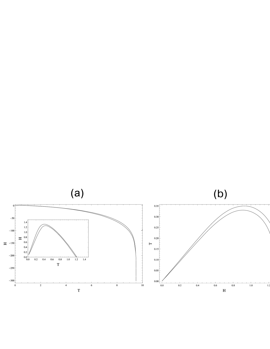
Figure 1: Fig. 1. Modulated period-3 phase for (a) the antiferromagnetic Potts model at $Q=1.1$, $J=1$, and $\gamma=3$ (inset shows the region $H>0$ at a magnified scale) and (b) the antiferromagnetic Ising model with three-site interaction at $J_{3}=-1$ and $\gamma=3$.

The antiferromagnetic Ising model with three-site interaction on the Husimi cactus in the presence of the external magnetic field [4] is specified by the Hamiltonian

$${\mathcal{H}}=-J_{3}\sum_{\bigtriangleup}\sigma_{i}\sigma_{j}\sigma_{k}-H\sum_{i}\sigma_{i},$$ (7)

where $\sigma_{i}=\pm 1$, the first sum is taken over all of the triangles, and second sum is calculated over all of the sites of the cactus, and $J_{3}<0$. In this case, the rational mapping and magnetization at the site of the central triangle are given by the expressions:

$$x_{n}=f_{2}(x_{n-1}),$$

$$f_{2}(x)=\frac{x^{2(\gamma-1)}e^{\frac{4H+2J_{3}}{T}}+2e^{\frac{2H}{T}}x^{\gamma-1}+e^{\frac{2J_{3}}{T}}}{2x^{\gamma-1}e^{\frac{2H+2J_{3}}{T}}+e^{\frac{4H}{T}}x^{2(\gamma-1)}+1},$$ (8)

$$M_{n}=\langle\sigma_{0}\rangle=\frac{e^{\frac{2H}{T}}x_{n}^{\gamma}-1}{e^{\frac{2H}{T}}x_{n}^{\gamma}+1},$$ (9)

where $x_{n}=j_{n}(\sigma_{0}=+1)/j_{n}(\sigma_{0}=-1)$ ($j_{n}$ is the contribution from each of $\gamma$ identical branches after cutting in the central triangle).

Thus, the $Q$-state Potts model on the Bethe lattice and the antiferromagnetic Ising model with three-site interaction on the Husimi cactus can be considered as nonlinear dynamical systems described by rational mappings. It is of interest to analyze the dependence of these rational mappings on both parameter $T$ (temperature) and parameter $H$ (external field) at a fixed coupling constant ($J$ or $J_{3}$), coordination number $\gamma$, and the number of states $Q$. The bifurcation points of the mappings correspond to the phase transition points with a change in symmetry.

We study the transition from the chaotic regime to the cyclic period-3 regime through tangent bifurcation [9]. Certain values of the temperature $T$ and magnetic field $H$ specify a curve separating the chaotic and period-3 regimes (the mapping in the latter regime has three stable stationary points). In this curve, tangent bifurcation occurs under the condition

$$\left\{\begin{array}[]{ll}f_{i}^{(3)}(x)=x&\\ (f_{i}^{(3)}(x))^{\prime}=1,(i=1,2),&\end{array}\right.$$ (12)

where $f^{(3)}(x)=f(f(f(x)))$. Subsequent bifurcations, responsible for the appearance of a stable cycle with a period of $3\times 2^{n}$ ($n=2,3,...$), correspond to the doubling of the period. For this reason, the next doubling bifurcation point can be found from the condition

$$\left\{\begin{array}[]{ll}f_{i}^{(3)}(x)=x&\\ (f_{i}^{(3)}(x))^{\prime}=-1,(i=1,2).&\end{array}\right.$$ (15)

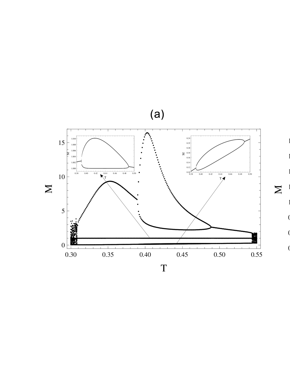
Figure 2: Fig. 2. Magnetization in the cyclic period-3 window for the Potts model at $Q=1.1$, $J=1$, and $\gamma=3$ (a) versus the temperature for $H=1.24$ (inset shows the details of the modulated period-six phase) and (b) versus the magnetic field for $T=1$.

The region bounded by curves found from conditions (12) and (15) corresponds to the modulated period-3 phase 3M0 (i.e., ${\bf 3}\times 2^{\bf 0}=3$) of the Potts model on the Bethe lattice at $i=1$ and the antiferromagnetic Ising model with three-site interaction on the Husimi cactus at $i=2$ (see Fig. 1). As is seen in the inset in Fig. 1a, the temperature dependencies of the mapping $f_{1}(x)$ and, hence, magnetization $M$ in the region $H\geq 0.1$ (curves specified by Eqs. (12) and (15) intersect at $H=0.1$), have interesting properties. When an $H=const$ line intersects only the upper curve (corresponding to Eq. (10) with $i=1$), the boundaries of the cyclic window are strictly distinguished (tangent bifurcation occurs at both edges). This window is represented only by the 3M0 phase (a stable period-3 cycle). As the fixed field decreases, when an $H=const$ line intersects both the upper curve (corresponding to Eq. (12) with $i=1$) and the lower curve (corresponding to Eq. (15) with $i=1$), a cycle with a period of $3\times 2^{1}=6$ appears, which corresponds to the modulated phase 3M1 ${\bf 3}\times 2^{\bf 1}=6$) with a period of 6 (see Fig. 2a). The phase transition between the 3M0 and 3M1 phases, accompanied by a change in symmetry, occurs at the bifurcation points. With a further decrease in the field, new bubbles corresponding to modulated phases with larger periods will appear on bifurcation diagrams. Finally, the chaotic regime, which is localized inside the cyclic period-3 window, will be reached. At the same time, when the magnetization is considered as a function of the temperature $T$ at a fixed value $H<0.1$ or as a function of the magnetic field $H$ at any fixed temperature, tangent bifurcation occurs only at one edge of the cyclic window [10]. A crisis [11, 12], i.e., the collision of the chaotic attractor with the independent unstable stationary point with a period of 3, occurs at the other edge (see Fig. 2b). In this case, modulated phases with a period of $3\times 2^{n}$ are not localized inside the window (similarity with logistic mapping).

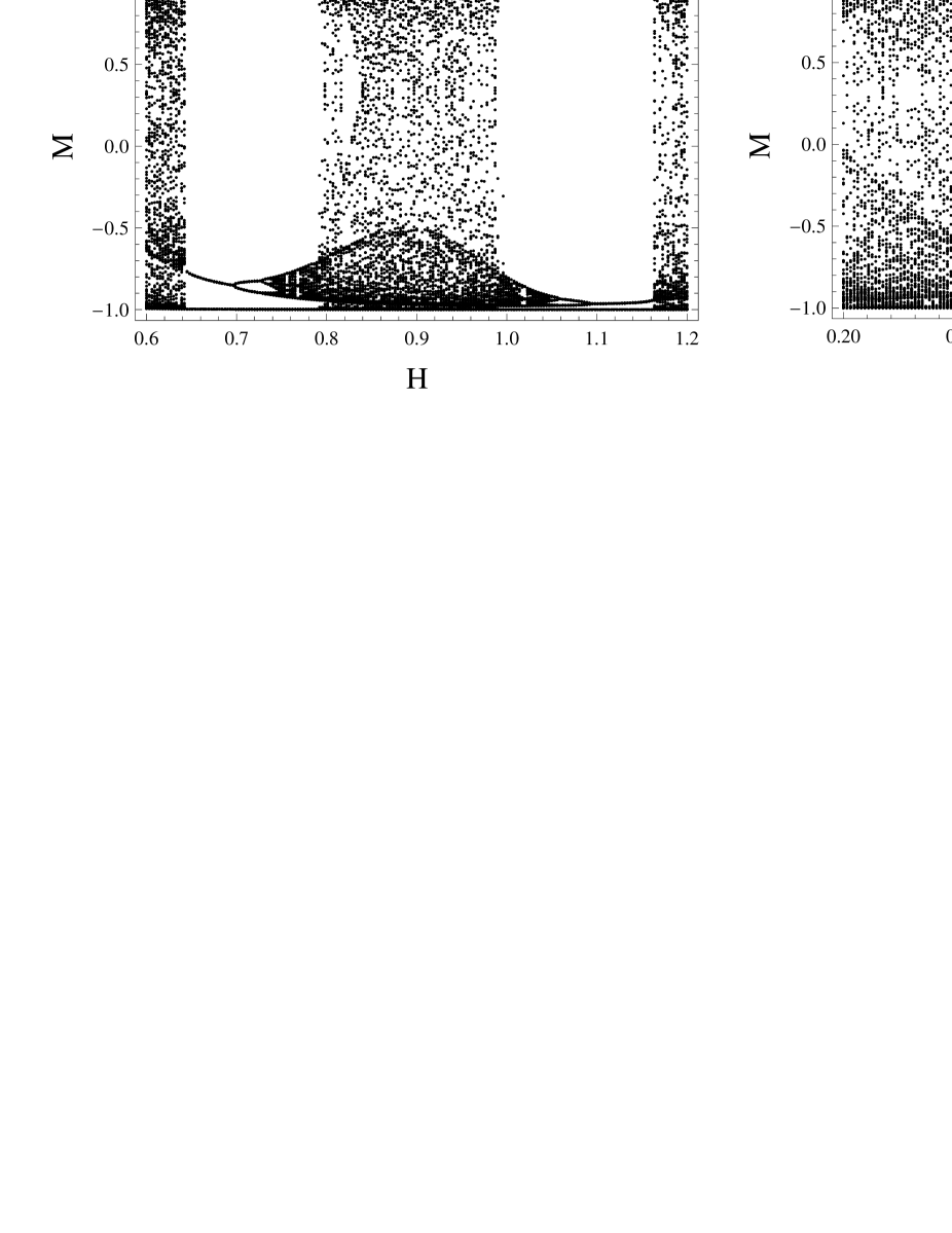
Figure 3: Fig. 3. Magnetization in the cyclic period-3 window for the antiferromagnetic Ising model with three-site interaction at $J_{3}=1$ and $\gamma=3$ (a) versus the magnetic field for $T=0.3$ and (b) versus the temperature for $H=0.5$.

The comparison of the picture described above with the behavior of the mapping $f_{2}(x)$ (therefore, the magnetization in the antiferromagnetic Ising model with three-site interaction) indicates that tangent bifurcation occurs at both edges of the window, when the temperature is fixed ($T=const$) and the external field is varied (see Fig. 1b). If a $T=const$ line intersects only the curve corresponding to Eq. (12) with $i=2$, the window is represented only by the 3M0 phase. When a $T=const$ line intersects the curve corresponding to Eq. (15) with $i=2$, there is also the 3M1 phase (in the form of a new bubble), transition to which occurs through doubling bifurcation (a phase transition with a change in symmetry). With a further decrease in the temperature, chaos is reached (as in the Potts model at $H=const$) inside the window (see Fig. 3a). This picture (localization of $3\times 2^{n}$ phases inside the cyclic period-3 window) for the rational mappings given by Eqs. (5) and (8), which describe statistical spin systems, was also observed in the three-dimensional (polynomial) Rossler system [12, 13].

At the same time, as is shown in Fig. 3b, the transition between chaos and the 3MO phase through tangent bifurcation in the antiferromagnetic Ising model with three-site interaction at a fixed field $H$ occurs only at one edge of the window. At the other edge of the window, an abrupt change in the chaotic attractor occurs due to crisis (as in the Potts model at a fixed temperature $T$). Thus, bifurcation properties in the cyclic period-3 window in the antiferromagnetic Potts model on the Bethe lattice in the dependence of the temperature $T$ at magnetic fields $H$ higher than those at the intersection point of the curves specified by Eqs. (12) and (15) ($H=0.1$ at $Q=1.1$) are similar to the respective properties of the Ising antiferromagnetic model with three-particle interaction on the Husimi cactus in the dependence of the magnetic field $H$ (see Fig. 1b and inset in Fig. 1a). However, there is a certain interval $H\in[1.276;1.375]$, where the ground state of the Ising antiferromagnetic model with three-particle interaction is the period-3 phase 3M0 (see Fig. 1b).

Concluding the discussion of the phase structure of the period-3 window, we consider the Lyapunov exponent $\lambda(x)$ as an order parameter. As is known, $\lambda(x)$ characterizes the degree of the exponential divergence of two neighboring points induced by the mapping $x_{n+1}=f(x_{n})$. The exact formula for $\lambda(x)$ has the form

$$\lambda{(x)}=\lim_{n\rightarrow\infty}{\frac{1}{n}}\ln\left|\frac{df^{(n)}(x)}{dx}\right|.$$ (16)

The Lyapunov exponent is negative in the periodic regime, positive in the chaotic regime, and zero at the bifurcation points. Figures 4a and 4b show the magnetic field and temperature dependencies of the Lyapunov exponents for $f_{1}(x)$ and $f_{2}(x)$, respectively, for the same remaining parameters as in Figs. 2a and 3b, respectively. According to Fig. 4, $\lambda(x)=-\infty$ at certain parameters $T$ and $H$. These points correspond to the superstable cycles [14],which are located in the region of the particular modulated phase. Therefore, the construction (both analytical and numerical) of the superstable cycle of the order $n$ will make it possible to determine the regions of $T$ and $H$ where the modulated phase of a period of $n$ exists. This problem will be considered in future works.

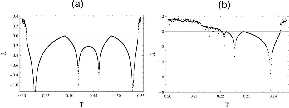
Figure 4: Fig. 4. Temperature dependence of the Lyapunov exponent in the cyclic period-3 window for (a) the Potts model at $Q=1.1$, $J=1$, $\gamma=3$, and $H=1.24$ and (b) the antiferromagnetic Ising model with three-site interaction at $J_{3}=1$, $\gamma=3$, and $H=0.5$.

Our calculations also show that the Feigenbaum constants $\alpha$ and $\delta$ for the doubling of the period [15] of the mappings $f_{1}(x)$ and $f_{2}(x)$ converge to the known universal values $\delta=4,6692...$ and $\alpha=2,5029...$, respectively. Convergence in the period-3 window (doubling of the period in the form $3\times 2^{n}$) is slower than that in the case of the doubling of the period in the form $1\times 2^{n}$. It is interesting that the universality of the Feigenbaum constants can also be used for the approximate construction of the curves of phase transitions between different modulated phases [10].

In summary, a cyclic period-3 window has been studied in the antiferromagnetic Potts model on the Bethe lattice and in the antiferromagnetic Ising model with three-site interaction on the Husimi cactus. The Bethe lattice and its generalizations are approximations for the standard lattices (Bethe-Peierls approximation), which is much more accurate than the mean field approximation. For rational mappings, which describe real statistical models (the antiferromagnetic $Q$-state Potts model on the Bethe lattice and the antiferromagnetic Ising model with three-site interaction on the Husimi cactus), we have analyzed the mechanism of the transition from the chaotic regime to the cyclic period-3 window through tangent bifurcation followed by the doubling cascade $3\times 2^{n}$ ($n=2,3,...$). The period-3 modulated phase of both models has been presented on the phase diagram. The Lyapunov exponents in the period-3 window have been calculated.

This work was supported by the Armenian National Foundation of Science and Advanced Technologies, project no. ECSP-09-08 SASP, and the Armenian National Science and Education Fund, project no. PS-2497.

References

- [1] R. J. Baxter, Exactly Solved Models in Statistical Mechanics (Academic Press, New York, 1982; Mir, Moscow, 1985); F. Y. Wu, Rev. Mod. Phys. 54, 235 (1982); N. S. Ananikyan and A. Z. Akheyan, Sov. Phys. JETP 80, 105 (1995).
- [2] R. F. S. Andrade and D. Cason, Phys. Rev. B81, 014204 (2010); T. Iharagi, A. Gendiar, H. Ueda et al., J. Phys. Soc. Jpn. 79, 104001 (2010).
- [3] J. L. Monroe, J. Stat. Phys. 65, 255 (1991); J. Phys. A29, 5421 (1996); N. S. Ananikyan, N. Sh. Izmailyan, and R. R. Shcherbakov, JETP Lett. 59, 71 (1994); N. S. Anankian, R. R. Lusiniants, and K. A. Oganissyan, JETP Lett. 61, 496 (1995).
- [4] R. A. Zara, M. Pretti, J. Chem. Phys. 127, 184902 (2007); M. Udagawa, H. Ishizuka and Y. Motome, Phys. Rev. Lett. 104, 226405 (2010); N. S. Ananikian, S. K. Dallakian, N. Sh. Izmailian et al., Fractals 5, 175 (1997).
- [5] T. R. Arakelyan, V. R. Ohanyan, L. N. Ananikyan, et al., Phys. Rev. B67, 024424 (2003); L. N. Ananikyan, Int. J. Mod. Phys. B21, 755 (2007); V. V. Hovhannisyan and N. S. Ananikian, Phys. Lett. A372, 3363 (2008).
- [6] D. V. Gal tsov and V. V. Dyadichev, JETP Lett. 77, 154 (2003); A. Y. Akheyan and N. S. Ananikian, J. Phys. A25, 3111 (1992); N. S. Ananikian, A. Z. Akheyan, and N. G. Ter-Arutyunyan-Savvidi, Teor. Mat. Fiz. 78, 281 (1989).
- [7] D. V. Vagin, O. P. Polyakov, J. Magn. Magn. Mater., 320, 3394 (2008); S. Ishii, M. -A. Sato, Neural Networks 10, 941 (1997); D. M. Maranhao, M. S. Baptista, J. C. Sartorelli et al., Phys. Rev. E77, 037202 (2008).
- [8] N. Ananikian, L. Ananikyan, R. Artuso et al., Phys. Lett. A374, 4084 (2010); C. Anteneodo, R. N. P. Maia, and R. O. Vallejos, Phys. Rev. E68, 036120 (2003); N. S. Ananikian, L .N. Ananikyan, R. Artuso et al., Physica D239, 1723 (2009).
- [9] P. Manneville, Y. Pomeau, Phys. Lett. A75, 1 (1979); Physica D1, 219 (1980); A. E. Hramov, A. A. Koronovskii, and M. K. Kurovskayaet, Phys. Rev. E76, 2 (2007); S. Chiriac, D. G. Dimitriu, and M. Sanduloviciu, Phys. Plasmas 14, 072309 (2007).
- [10] L. N. Ananikyan, N. S. Ananikian, and L. A. Chakhmakhchyan, Fractals 18, 371 (2010).
- [11] C. Grebogi, E. Ott, J. A. Yorke, Physica D7, 181 (1983).
- [12] S. Zambrano, I. P. Marino, and M. A. F Sanjuán, New J. Phys. 11, 023025 (2009).
- [13] A. P. Kuznetsov, N. V. Stankevich, and L. V. Tyuryukina, Tech. Phys. Lett. 34, 618 (2008).
- [14] J. Guckenheimer, G. Oster, and A. Ipaktchi, J. Math. Biol. 4, 101 (1977); W. B. Gordon, Math. Mag. 69, 118 (1996); M. H. Lee, J. Math. Phys. 50, 122702 (2009).
- [15] M. J. Feigenbaum, J. Stat. Phys. 19, 25 (1978); 21, 669 (1979); E. B. Vul, Ya. G. Sinai, K. M. Khanin, Usp. Mat. Nauk 39, 3 (1984).