Geometry of the shears mechanism in nuclei

Abstract

The geometry of the shears mechanism in nuclei is derived from the nuclear shell model. This is achieved by taking the limit of large angular momenta (classical limit) of shell-model matrix elements.

A central theme in the study of quantum many-body systems is the understanding of its elementary modes of excitation. Of particular interest is the competition between single-particle and collective degrees of freedom. In general, single-particle motion gives rise to irregular level sequences, associated with the unique properties of the individual particles. Collective motion generates more regular structures, a typical example being that of rotational bands which follow closely a $J(J+1)$ sequence, characteristic of a quantum rotor.

In atomic nuclei, the energy scales of these modes are somewhat comparable, leading to a rich and complex structure BM75 . ²⁰⁸Pb is considered a paradigm of a doubly-closed-shell nucleus with collective states based on an octupole phonon. Neighboring nuclei provided a wealth of important information for the shell model, on single-particle levels and residual interactions at the $Z=82$, $N=126$ shell closure, as well as on the role of particle-vibration coupling Hamamoto74 .

The observation in ¹⁹⁹Pb of a regular sequence of $\gamma$ rays resembling, at first look, a rotational band came as a surprise Baldsiefen92 ; Clark92 ; Clark00 ; Hubel05 . A closer inspection of the data established that these transitions were of magnetic character, in contrast to the quadrupole nature in the well-known nuclear rotors BM75 . The answer to this puzzle was provided by Frauendorf Frauendorf93 , who based on the Titled Axis Cranking Model proposed the so-called “shears mechanism”. He showed that for a weakly deformed system, there exist low-energy configurations in which neutrons and protons combine into stretched structures (“blades”) and the angular momentum is generated by the re-coupling of these blades, resembling the closing of a pair of shears. As discussed in Ref. Frauendorf01 , the breaking of the rotational symmetry in this case originates in an anisotropic distribution of nucleonic current loops (rather than electric charge), and thus it is usually referred as magnetic rotation. Further experiments not only confirmed this picture in the lead region, but also established the mechanism in other regions of the Segré chart, near doubly-magic closures.

While an interpretation in terms of the shears mechanism provides an appealing, intuitive picture of these nuclear states, the question remains whether this geometric character is borne out by microscopic calculations. In numerical shell-model calculations Frauendorf et al. Frauendorf96 showed that the shears picture is valid in the lead isotopes. A direct derivation of the geometry of the shears mechanism from the shell model has, however, to our knowledge never been given. Providing such a derivation is the purpose of the present Letter.

Let us assume that two nucleons of one type (say neutrons) occupy particle-like orbits $j_{1\nu}$ and $j_{2\nu}$, while two nucleons of the other type (protons) occupy hole-like orbits $j_{1\pi}^{-1}$ and $j_{1\pi}^{-1}$ note1 . The neutrons and protons are coupled to angular momenta $J_{\nu}$ and $J_{\pi}$, respectively, which are close to stretched, $J_{\rho}\approx j_{1\rho}+j_{2\rho}$ ($\rho=\nu,\pi$). The two-particle (2p) and two-hole (2h) states are represented as $|N\rangle=|j_{1\nu}j_{2\nu};J_{\nu}\rangle$ and $|P^{-1}\rangle=|j_{1\pi}^{-1}j_{2\pi}^{-1};J_{\pi}\rangle$, and we assume that the states are Pauli allowed, i.e., that $J_{\rho}$ is even if $j_{1\rho}=j_{2\rho}$. A shears band consists of the states $|NP^{-1};J\rangle$ where $J$ results from the coupling of $J_{\nu}$ and $J_{\pi}$.

We ask the following questions: How do the energies of the members of this band evolve as a function of $J$, and how does this evolution depends on the angular momenta of the single-particle orbits and the angular momenta of the blades? We answer these questions by adopting a shell-model hamiltonian of the generic form $H=H_{\nu}+H_{\pi}+V_{\nu\pi}$ and computing $\langle NP^{-1};J|H|NP^{-1};J\rangle$, which will be referred to as the (2p-2h) shears matrix element.

The shell-model hamiltonian is specified by the single-particle energies, the single-hole energies, the neutron-neutron and proton-proton (two-body) interaction matrix elements, and the neutron-proton (np) interaction matrix elements $V_{j_{\nu}j_{\pi}}^{R}\equiv\langle j_{\nu}j_{\pi};R|V_{\nu\pi}|j_{\nu}j_{\pi};R\rangle$. One finds that the energy contribution of $H_{\nu}$ and $H_{\pi}$ is constant for all members of the shears band and that any $J$ dependence originates from the np interaction $V_{\nu\pi}$. A multipole expansion of the latter interaction leads to the following expression for the shears matrix element:

$$\langle NP^{-1};J|V_{\nu\pi}|NP^{-1};J\rangle$$ (4)

$$= -{\cal P}\hat{J}_{\nu}\hat{J}_{\pi}\sum_{R}\hat{R}\,V_{j_{1\nu}j_{1\pi}}^{R}\left\{\begin{array}[]{cccccccc}\!\!j_{1\nu}\!\!\!\!&&\!\!J_{\nu}\!\!&&\!\!J_{\pi}\!\!&&\!\!j_{1\pi}\!\!\!\!&\\ &\!\!j_{2\nu}\!\!\!\!&&\!\!J\!\!&&\!\!j_{2\pi}\!\!\!\!&&\!\!R\!\!\\ \!\!j_{1\nu}\!\!\!\!&&\!\!J_{\nu}\!\!&&\!\!J_{\pi}\!\!&&\!\!j_{1\pi}\!\!\!\!&\end{array}\right\},$$

where $\hat{x}\equiv 2x+1$ and ${\cal P}\equiv{\cal P}_{\nu}{\cal P}_{\pi}$ with ${\cal P}_{\rho}$ an operator defined from ${\cal P}_{\rho}f(j_{1\rho},j_{2\rho})=f(j_{1\rho},j_{2\rho})+f(j_{2\rho},j_{1\rho})$ for any function $f$. The object in curly brackets is a 12$j$ symbol of the first kind, a quantity which is scalar under rotations and depends on twelve angular momenta. The result (4) is obtained by expressing the shears matrix element as a sum over four 6$j$ symbols, which can be related to a 12$j$ symbol, see Eq. (19.1) of Ref. Yutsis62 .

It is now a simple matter to introduce in the sum (4) values for the np interaction matrix elements and to derive the $J$ dependence of the shears matrix element. For any reasonable nuclear interaction and for $J_{\rho}\approx j_{1\rho}+j_{2\rho}$, it is found that the sum (4) has an approximate parabolic behavior around its minimum around $J^{2}\approx J_{\nu}^{2}+J_{\pi}^{2}$.

To understand better this numerical finding, the geometry of the expression (4) can be studied by taking the limit of large angular momenta in the recoupling coefficients. Such limits are known since the seminal study of Wigner on the classical limit of $3j$ and $6j$ symbols (see chapter 27 of Ref. Wigner59 ), subsequently refined by Ponzano and Regge Ponzano68 whose work was put on a mathematically solid footing by Schulten and Gordon Schulten75 . The classical limit of a $3j$ symbol is associated with the area of a (projected) triangle while that of a $6j$ symbol involves the volume of a tetrahedron, with the lengths of the sides determined by the angular momenta. Classical limits not only yield approximate expressions for (re)coupling coefficients but in addition provide an insight into their geometrical significance. The study of the classical limit of $3nj$ symbols with $n>2$ is still a topic of active research with ramifications in fields as diverse as quantum gravity and quantum computing (see, e.g. Refs. Anderson08 ; Anderson09 ; Haggard10 and references therein), well beyond the standard applications in, for example, atomic or nuclear physics.

Since at this moment only partial results are known for $9j$ (let alone $12j$) symbols, a classical limit of the expression (4) for arbitrary interactions is difficult to obtain. We consider instead the surface delta interaction (SDI) Brussaard77 , $V^{\rm SDI}(i,j)=-4\pi a^{\prime}_{T}\delta(\bar{r}_{i}-\bar{r}_{j})\delta(r_{i}-R)$, which is known to be a reasonable approximation to the nucleon-nucleon interaction note2 . The np matrix element $V_{j_{\nu}j_{\pi}}^{R}$ of the SDI is Brussaard77

$$-\frac{\hat{\jmath}_{\nu}\hat{\jmath}_{\pi}}{2}\left[a_{01}\left(\begin{array}[]{ccc}j_{\nu}&j_{\pi}&R\\ {\frac{1}{2}}&-{\frac{1}{2}}&0\end{array}\right)^{2}+a_{0}\left(\begin{array}[]{ccc}j_{\nu}&j_{\pi}&R\\ {\frac{1}{2}}&{\frac{1}{2}}&-1\end{array}\right)^{2}\right],$$ (5)

with $a_{01}=(a_{0}+a_{1})/2-(-)^{\ell_{\nu}+\ell_{\pi}+R}(a_{0}-a_{1})/2$ in terms of the strengths $a_{T}=a^{\prime}_{T}C(R_{0})$, where $C(R_{0})$ equals $R_{n_{\nu}\ell_{\nu}}^{4}(R_{0})R_{0}^{2}=R_{n_{\pi}\ell_{\pi}}^{4}(R_{0})R_{0}^{2}$.

When the SDI np matrix elements (5) are introduced in the shears matrix element (4), one encounters sums of the type

$$\sigma_{n}^{(\lambda)}\equiv(2J_{\nu}+1)(2J_{\pi}+1)\sum_{R}(-)^{\lambda R}(2R+1)\left(\begin{array}[]{ccc}j_{1\nu}&j_{1\pi}&R\\ {\frac{1}{2}}&n-{\frac{1}{2}}&-n\end{array}\right)^{2}\left\{\begin{array}[]{cccccccc}\!\!j_{1\nu}\!\!\!\!&&\!\!J_{\nu}\!\!&&\!\!J_{\pi}\!\!&&\!\!j_{1\pi}\!\!\!\!&\\ &\!\!j_{2\nu}\!\!\!\!&&\!\!J\!\!&&\!\!j_{2\pi}\!\!\!\!&&\!\!R\!\!\\ \!\!j_{1\nu}\!\!\!\!&&\!\!J_{\nu}\!\!&&\!\!J_{\pi}\!\!&&\!\!j_{1\pi}\!\!\!\!&\end{array}\right\},$$ (6)

for $(\lambda,n)=(0,0)$, (0,1) and (1,0). These reduce to simple expressions in the classical limit. For example, for $\lambda=0$, the sum can be exactly rewritten as

$$\sigma_{n}^{(0)}=(2J_{\nu}+1)(2J_{\pi}+1)\sum_{\stackrel{{\scriptstyle\scriptstyle m_{\nu}M_{\nu}}}{{m_{\pi}M_{\pi}}}}\left(\begin{array}[]{ccc}j_{1\nu}&j_{2\nu}&J_{\nu}\\ {\frac{1}{2}}&m_{\nu}&M_{\nu}\end{array}\right)^{2}\left(\begin{array}[]{ccc}j_{1\pi}&j_{2\pi}&J_{\pi}\\ -n+{\frac{1}{2}}&m_{\pi}&M_{\pi}\end{array}\right)^{2}\left(\begin{array}[]{ccc}J_{\nu}&J_{\pi}&J\\ M_{\nu}&M_{\pi}&m_{\nu}+m_{\pi}-n+1\end{array}\right)^{2}.$$ (7)

The classical approximation consists of replacing the last $3j$ symbol in Eq. (7) according to Wigner59

$$\left(\begin{array}[]{ccc}J_{\nu}&J_{\pi}&J\\ M_{\nu}&M_{\pi}&M\end{array}\right)^{2}\mapsto\left(4\pi A^{J_{\nu}J_{\pi}J}_{M_{\nu}M_{\pi}M}\right)^{-1},$$ (8)

where $A^{J_{\nu}J_{\pi}J}_{M_{\nu}M_{\pi}M}$ is related to the Caley determinant,

$$\left(A^{J_{\nu}J_{\pi}J}_{M_{\nu}M_{\pi}M}\right)^{2}=-\frac{1}{16}\left|\begin{array}[]{cccc}0&a_{J_{\nu}M_{\nu}}&a_{J_{\pi}M_{\pi}}&1\\ a_{J_{\nu}M_{\nu}}&0&a_{JM}&1\\ a_{J_{\pi}M_{\pi}}&a_{JM}&0&1\\ 1&1&1&0\end{array}\right|,$$ (9)

with $a_{JM}\equiv(J+{\frac{1}{2}})^{2}-M^{2}$. While the $3j$ symbol in Eq. (8) usually is a rapidly oscillating function of $M_{\nu}$ and $M_{\pi}$, its classical approximation is smooth. Many oscillations occur except when $J$ is close to its minimum or maximum value, $J=|J_{\nu}-J_{\pi}|$ or $J=J_{\nu}+J_{\pi}$, respectively. The approximation (8) in the sum (7), therefore, can be expected to be reasonable in most cases, in particular in the region of physics interest where $J^{2}\approx J_{\nu}^{2}+J_{\pi}^{2}$. Since $J_{\rho}\approx j_{1\rho}+j_{2\rho}$, a classical approximation cannot be made for the first two $3j$ symbols in Eq. (7). From the explicit expressions for the $3j$ symbols one can show that the sum over $M_{\nu}$ and $M_{\pi}$ can be restricted to the region around $M_{\nu}=M_{\pi}=0$. Since the classical approximation (8) is nearly constant for small values of $M_{\nu}$ and $M_{\pi}$, the classical limit for the $3j$ symbols with zero projections on the $z$ axis can be taken, to obtain

$$\sigma_{0}^{(0)}\approx\sigma_{1}^{(0)}\approx\frac{(2J_{\nu}+1)(2J_{\pi}+1)}{4\pi(2j_{1\nu}+1)(2j_{1\pi}+1)A},$$ (10)

where $A\equiv A^{J_{\nu}J_{\pi}J}_{000}$ is the area of a triangle with sides of lengths $J_{\nu}+{\frac{1}{2}}$, $J_{\pi}+{\frac{1}{2}}$, and $J+{\frac{1}{2}}$ note3 . We may alternatively express this sum in terms of the shears angle,

$$\theta_{\nu\pi}=\arccos\frac{J(J+1)-J_{\nu}(J_{\nu}+1)-J_{\pi}(J_{\pi}+1)}{2\sqrt{J_{\nu}(J_{\nu}+1)J_{\pi}(J_{\pi}+1)}},$$ (11)

leading to

$$\sigma_{0}^{(0)}\approx\sigma_{1}^{(0)}\approx\frac{2}{\pi(2j_{1\nu}+1)(2j_{1\pi}+1)\sin\theta_{\nu\pi}}.$$ (12)

A similar derivation yields the classical approximation

$$\sigma_{0}^{(1)}\approx-(-)^{j_{\nu}+j_{\pi}}\frac{2}{\pi(2j_{1\nu}+1)(2j_{1\pi}+1)\tan\theta_{\nu\pi}}.$$ (13)

Introducing the preceding approximations into the expression for the shears matrix element (4), we obtain

$$\langle NP^{-1};J|V_{\nu\pi}^{\rm SDI}|NP^{-1};J\rangle\approx\frac{s_{2}}{2\pi\sin\theta_{\nu\pi}}+\frac{t_{2}}{2\pi\tan\theta_{\nu\pi}},$$ (14)

where

$$s_{2}=4(3a_{0}+a_{1}),\qquad t_{2}=\varphi(a_{0}-a_{1}),$$

$$\varphi={\cal P}(-)^{\ell_{1\nu}+j_{1\nu}+\ell_{1\pi}+j_{1\pi}}.$$ (15)

The classical limit of the shears matrix element for the SDI does not depend on the individual single-particle angular momenta but only on the shears angle, which is defined by the angular momenta $J_{\nu}$ and $J_{\pi}$ of the blades and the total angular momentum $J$.

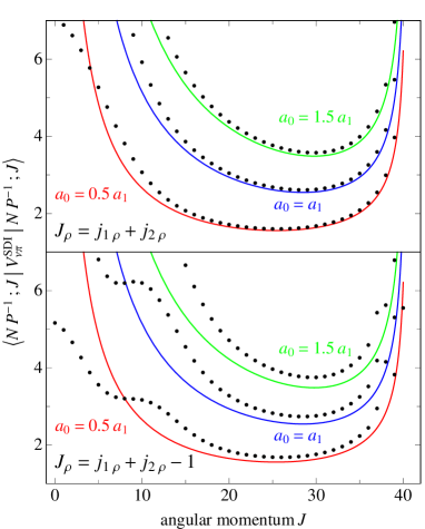
Figure 1: The exact expression (4) for the 2p-2h shears matrix element of the SDI (dots) compared with its classical approximation (14) (lines) for neutron and proton angular momenta $J_{\nu}=J_{\pi}=20$. The single-particle angular momenta are $j_{1\rho}=\frac{19}{2}$ and $j_{2\rho}=\frac{21}{2}$ (top), and $j_{1\rho}=j_{2\rho}=\frac{21}{2}$ (bottom). Results are shown for three choices of the ratio $a_{0}/a_{1}$. The matrix element is in units $a_{1}$.

In Fig. 1 the exact shears matrix elements of the SDI are compared with their classical approximation for the neutron and proton angular momenta of the blades $J_{\nu}=J_{\pi}=20$. The approximation is good for the stretched case, $J_{\rho}=j_{1\rho}+j_{2\rho}$, but deteriorates rapidly as $J_{\rho}$ diminishes. However, in the region of interest, where the two angular momenta $J_{\nu}$ and $J_{\pi}$ are close to orthogonal, $J^{2}\approx J_{\nu}^{2}+J_{\pi}^{2}$, the classical approximation is good, also for $J_{\rho}=j_{1\rho}+j_{2\rho}-1$, and the geometric picture underlying the shears mechanism remains valid.

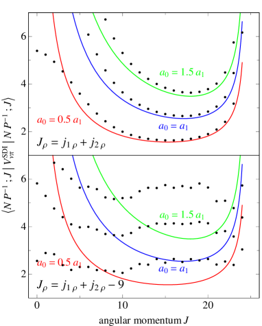
Figure 2: Same as Fig. 1 for neutron and proton angular momenta $J_{\nu}=J_{\pi}=12$ and single-particle angular momenta $j_{1\rho}=\frac{11}{2}$ and $j_{2\rho}=\frac{13}{2}$ (top), and $j_{1\rho}=j_{2\rho}=\frac{21}{2}$ (bottom).

This analysis also reveals the limits of the validity of this geometric picture, as is illustrated in Fig. 2 which shows the shears matrix element of the SDI for the neutron and proton angular momenta $J_{\nu}=J_{\pi}=12$. In one case these arise from aligned single-particle angular momenta ($j_{1\rho}=\frac{11}{2}$ and $j_{2\rho}=\frac{13}{2}$) and the classical approximation is seen to be reasonable. In the second case the single-particle angular momenta are larger ($j_{1\rho}=j_{2\rho}=\frac{21}{2}$) and they are not aligned ($J_{\rho}=j_{1\rho}+j_{2\rho}-9$), leading to a breakdown of the shears interpretation. The alignment of the particles in high-$j$ orbits, introduced here by hand, is in a more realistic shell-model calculation due to their interaction with particles in low-$j$ orbits Frauendorf96 .

The classical expression (14) is reminiscent of the interpretation of nuclear matrix elements in terms of the angle between the vectors of the single-particle angular momenta (see, e.g., Schiffer and True Schiffer76 ). In fact, it can be shown that the classical limit of the 1p-1h matrix element $\langle j_{\nu}j_{\pi}^{-1};J|V_{\nu\pi}^{\rm SDI}|j_{\nu}j_{\pi}^{-1};J\rangle$ leads to the same dependence on the angle $\theta_{\nu\pi}$ as in Eq. (14) but with coefficients $s_{1}$ and $t_{1}$ that depend differently on the strengths $a_{T}$ of the interaction.

The present results make contact with the semi-classical analysis Clark00 ; Hubel05 in terms of an interaction $V_{0}+V_{2}P_{2}(\cos\theta_{\nu\pi})$, assumed to exist between the blades of the shears bands. In line with the intuitive picture one has of the shears mechanism, this interaction necessarily implies a shears-band head with $\cos\theta_{\nu\pi}^{\rm 0}\approx 0$ or, alternatively, a minimum energy for $J^{2}\approx J_{\nu}^{2}+J_{\pi}^{2}$ when the angular momentum vectors $\bar{J}_{\nu}$ and $\bar{J}_{\pi}$ are orthogonal. Our analysis shows that this is not generally valid since a minimum energy is obtained from Eq. (14) for $\cos\theta_{\nu\pi}^{\rm 0}\approx-t_{2}/s_{2}=\varphi(a_{1}-a_{0})/4(3a_{0}+a_{1})$. Therefore, if the isoscalar and isovector interaction strengths are different, a minimum energy is found for a non-orthogonal configuration.

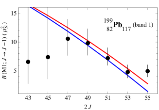
Figure 3: Experimental (points) and calculated (lines) $B$(M1) values for band 1 in ¹⁹⁹Pb as a function of twice the angular momentum $J$. The red line is the exact expression and the blue line is its classical limit (16).

Shears bands are characterized by strong M1 transitions that decrease with increasing angular momentum $J$. For a general configuration $|NP^{-1};J\rangle$, where $|N\rangle$ is an $m$-particle neutron and $|P^{-1}\rangle$ an $m^{\prime}$-hole proton configuration with angular momenta $J_{\nu}$ and $J_{\pi}$, respectively, standard recoupling techniques Talmi93 lead to the following classical expression for the $B$(M1) values:

$$B({\rm M1};J\rightarrow J-1)$$ (16)

$$\approx \frac{3}{4\pi}(g_{\nu}-g_{\pi})^{2}\frac{(2J_{\nu}+1)^{2}(2J_{\pi}+1)^{2}}{16J(2J+1)}\sin^{2}\theta_{\nu\pi},$$

where $g_{\nu}$ and $g_{\pi}$ are the $g$ factors of the neutron and proton configurations $|N\rangle$ and $|P^{-1}\rangle$, respectively. This expression can be tested in ¹⁹⁹Pb where lifetimes of some shears-band levels have been measured Neffgen95 . In particular, the states in band 1 with $\frac{43}{2}<J<\frac{55}{2}$ have the suggested Baldsiefen94 configuration $\nu(1i_{13/2}^{-3})_{33/2}\times\pi(1h_{9/2}1i_{13/2})_{11}$, from where the $g$ factors can be obtained, $g_{\nu}=-0.29~{}\mu_{\rm N}$ and $g_{\pi}=1.03~{}\mu_{\rm N}$. Application of Eq. (16) with $J_{\nu}=\frac{33}{2}$ and $J_{\pi}=11$ leads to the result shown in Fig. 3 (in blue), which is seen to be close to the exact result (in red). In the spin region $\frac{47}{2}\leq J\leq\frac{53}{2}$, where the above configuration is thought to apply, agreement is obtained.

The data on M1 transitions indicate that fixed neutron and proton configurations do not apply to an entire shears band but only to part of it. For this reason it will be difficult to use energy formulas like Eq. (14) with constant coefficients $s_{2}$ and $t_{2}$ for an entire band. The present analysis suggests however that, under certain conditions of angular-momentum alignment, the generic form of the expression (14) is approximately valid with coefficients $s_{i}$ and $t_{i}$ depending on the structure of the neutron and proton configurations that apply to certain ranges of the total angular momentum $J$. This problem is currently under study.

This work was partially supported (AOM) by the Director, Office of Science, Office of Nuclear Physics, of the U.S. Department of Energy under contract No. DE-AC02-05CH11231 and by FUSTIPEN (French-U.S. Theory Institute for Physics with Exotic Nuclei) under DOE grant No. DE-FG02-10ER41700.

References

- (1) A. Bohr and B.R. Mottelson, Nuclear Structure. II Nuclear Deformations (Benjamin, New York, 1975).
- (2) I. Hamamoto, Phys. Reports 10, 63 (1974).
- (3) G. Baldsiefen et al., Phys. Lett. B 275, 252 (1992).
- (4) R.M. Clark et al., Phys. Lett. B 275, 247 (1992).
- (5) R.M. Clark and A.O. Macchiavelli, Annual Rev. Nucl. Part. Sci. 50, 1 (2000).
- (6) H. Hubel, Progr. Part. Nucl. Phys. 54, 1 (2005).
- (7) S. Frauendorf, Nucl. Phys. A 557, 259c (1993).
- (8) S. Frauendorf, Rev. Mod. Phys. 73, 463 (2001).
- (9) S. Frauendorf, J. Reif, and G. Winter, Nucl. Phys. A 601, 41 (1996).
- (10) The notation is used as an abbreviation for the set of quantum numbers , , and of singe-particle levels in a central potential.
- (11) A.P. Yutsis, I.B. Levinson, and V.V. Vanagas, The Theory of Angular Momentum (Israel Program for Scientific Translations, Jerusalem, 1962).
- (12) E.P. Wigner, Group Theory and Its Application to the Quantum Mechanics of Atomic Spectra (Academic Press, New York, 1959).
- (13) G. Ponzano and T. Regge, Spectroscopy and Group Theoretical Methods in Physics (North-Holland, Amsterdam, 1968).
- (14) K. Schulten and R.G. Gordon, J. Math. Phys. 16, 1971 (1975).
- (15) R.W. Anderson, V. Aquilanti, and C. da Silva Ferreira, J. Chem. Phys. 129, 161101 (2008).
- (16) R.W. Anderson, V. Aquilanti, and A. Marzuoli, J. Phys. Chem. A 113, 15106 (2009).
- (17) H.M. Haggard and R.G. Littlejohn, Class. Quantum Grav. 27, 135010 (2010).
- (18) P.J. Brussaard and P.W.M. Glaudemans, Shell-Model Applications in Nuclear Spectroscopy (North-Holland, Amsterdam, 1977).
- (19) The modified SDI which includes an charge exchange and a constant term is a better approximation still Brussaard77 . It can be shown, however, that these extra terms do not affect the relative energies of the shears-band members.
- (20) In the original discussion of the classical limit of the symbol, chapter 27 of Ref. Wigner59 , is neglected with respect to the lengths of the angular-momentum vectors. It is added here, in line with subsequent discussions, e.g. Ref. Schulten75 .
- (21) J.P. Schiffer and W.W. True, Rev. Mod. Phys. 48, 191 (1976).
- (22) I. Talmi, Simple Models of Complex Nuclei. The Shell Model and the Interacting Boson Model (Harwood, Chur, 1993).
- (23) M. Neffgen et al., Nucl. Phys. A 595, 499 (1995).
- (24) G. Baldsiefen et al., Nucl. Phys. A 574, 521 (1994).