Alfvén Wave Collisions, The Fundamental Building Block of Plasma Turbulence IV: Laboratory Experiment

Abstract

Turbulence is a phenomenon found throughout space and astrophysical plasmas. It plays an important role in solar coronal heating, acceleration of the solar wind, and heating of the interstellar medium. Turbulence in these regimes is dominated by Alfvén waves. Most turbulence theories have been established using ideal plasma models, such as incompressible MHD. However, there has been no experimental evidence to support the use of such models for weakly to moderately collisional plasmas which are relevant to various space and astrophysical plasma environments. We present the first experiment to measure the nonlinear interaction between two counterpropagating Alfvén waves, which is the building block for astrophysical turbulence theories. We present here four distinct tests that demonstrate conclusively that we have indeed measured the daughter Alfvén wave generated nonlinearly by a collision between counterpropagating Alfvén waves.

I Introduction

Plasma turbulence is important for our understanding of the dynamics of various space and astrophysical plasma environments, including the heating of the interstellar medium, Spangler and Cordes (1998) acceleration of the solar wind,Verdini and Velli (2010); Bingham et al. (2010) solar coronal heating,Cranmar and van Ballegooijen (2003) transport of energy and mass into Earth’s magnetosphere,Lee, Johnson, and Ma (1994); Sundkvist et al. (2005) and heat transport in galaxy clusters.Peterson and Fabian (2006); Lazarian (2006) Although these seem to be strikingly different environments, the turbulence in these plasmas is dominated by Alfvén waves, which are low frequency, large length scale waves. This turbulent interaction arises when two counterpropagating Alfvén waves interact nonlinearly in the plasma medium. This nonlinear interaction, often referred to as a wave-wave collision, is the central component of astrophysical turbulence and is responsible for the turbulent cascade of energy from large to small scales.Schekochihin et al. (2009) In order to gain insight into this fundamental building block of astrophysical turbulence, experimental or observational measurements of the nonlinear interaction between two colliding Alfvén waves are essential.

Turbulent fluctuations in the solar wind Matthaeus and Goldstein (1982); Goldstein et al. (1995); Tu and Marsch (1995); Alexandrova et al. (2008); Sahraoui et al. (2009); Spangler, Savage, and Redfield (2011) and the interstellar medium Duffet-Smith and Readhead (1975); Rickett (1990); Gwinn, Bartel, and Cordes (1993); Scalo and Elmegreen (2004); Spangler, Savage, and Redfield (2010) have been measured for several decades. However, these measurements are mostly used to study the effect of turbulence on the plasma environment. Although characterization of the effects of turbulence on these environments is important, they do little to explain the physical mechanisms comprising the turbulence. More importantly, most of this data is limited by the fact that these are single-point measurements and, therefore, do not provide enough information about the 3-D structure of the turbulent fluctuations that leads to energy cascades from large to small scales.

In contrast to observations by spacecraft missions and telescopes, the controlled nature of laboratory experiments allows for more detailed measurements of the small-scale nonlinear interactions between Alfvén waves. In this paper, we provide detailed information about the experimental setup, experimental procedure, and data analysis of the first successful effort to confirm this nonlinear interaction, as outlined in Howes et al. (2012) In Sec. II, we briefly discuss the underlying theory. A more detailed theory can be found in the three companion papers by Howes and Nielson (2013), hereafter Paper I, Howes, Nielson, and Dorland (2013), hereafter Paper II, and Howes et al. (2013), hereafter Paper III. In Sec. III, we describe the experimental approach, with an emphasis on the two antennas used to produce the two counterpropagating Alfvén waves. In Sec. IV, we present an analysis of the experimental results, directly comparing the measured nonlinear signal to the predicted results from the theory.

II Alfvén wave turbulence theory

As shown in Paper I, the equations of incompressible MHD can be written in a symmetrized Elsässer form,(Elsasser, 1950)

$$\frac{\partial\mathbf{z}^{\pm}}{\partial t}\mp\mathbf{v}_{A}\cdot\nabla\mathbf{z}^{\pm}=-\mathbf{z}^{\mp}\cdot\nabla\mathbf{z}^{\pm}-\nabla P/\rho_{0},$$ (1)

$$\nabla\cdot\mathbf{z}^{\pm}=0$$ (2)

where the magnetic field is decomposed into equilibrium and fluctuating parts $\mathbf{B}=\mathbf{B}_{0}+\delta\mathbf{B}$, $\mathbf{v}_{A}=\mathbf{B}_{0}/\sqrt{4\pi\rho_{0}}$ is the Alfvén velocity due to the equilibrium field $\mathbf{B}_{0}=B_{0}\mbox{$\hat{\mathbf{z}}$}$, $P$ is total pressure (thermal plus magnetic), $\rho_{0}$ is mass density, and $\mathbf{z}^{\pm}(x,y,z,t)=\mathbf{u}\pm\delta\mathbf{B}/\sqrt{4\pi\rho_{0}}$ are the Elsässer fields given by the sum and difference of the velocity fluctuation $\mathbf{u}$, and the magnetic field fluctuation $\delta\mathbf{B}$ expressed in velocity units. This symmetrized Elsässer form of the incompressible MHD equations lends itself to a particularly simple physical interpretation. An Alfvén wave traveling down (up) the equilibrium magnetic field is represented by the Elsässer field $\mathbf{z}^{+}$ ($\mathbf{z}^{-}$). The second term on the left-hand side of Eq. (1) is the linear term representing the propagation of the Elsässer fields along the mean magnetic field at the Alfvén speed, the first term on the right-hand side is the nonlinear term representing the interaction between counterpropagating waves, and the second term on the right-hand side is a nonlinear term that ensures incompressibility.Montgomery (1982); Goldreich and Sridhar (1995); Howes and Nielson (2013)

As emphasized in Paper III, the mathematical properties of Eqs. (1) and (2) dictate that the fundamental building block of turbulence in an incompressible MHD plasma is the nonlinear interaction between perpendicularly polarized, counterpropagating Alfvén waves. Additionally, the strength of the nonlinear distortion of an Alfvén wave $\mathbf{z}^{+}$ traveling down the equilibrium magnetic field is controlled by the amplitude of the counterpropagating Alfvén wave $\mathbf{z}^{-}$ traveling up the magnetic field. Therefore, to measure the nonlinear energy transfer in an Alfvén wave collision, one need only launch a single Alfvén wave of large amplitude and then observe its effect on a counterpropagating Alfvén wave of smaller amplitude.

Instrumental limitations on the amplitude of Alfvén waves launched in the experiment lead to a situation in which the nonlinear terms on the right-hand side of Eq. (1) are small compared to the linear term on the left-hand side. Therefore, the experimental dynamics falls into the weakly nonlinear limit, and we can exploit the developments in the theory of weak MHD turbulenceIroshnikov (1963); Kraichnan (1965); Shebalin, Matthaeus, and Montgomery (1983); Sridhar and Goldreich (1994); Montgomery and Matthaeus (1995); Ng and Bhattacharjee (1996); Goldreich and Sridhar (1997); Galtier et al. (2000); Lithwick and Goldreich (2003) to optimize the experimental design, as discussed in detail in Paper III and briefly outlined in the remainder of this section.

Consider the case of the nonlinear interaction between two counterpropagating plane Alfvén waves with wavevectors $\mathbf{k}_{1}$ and $\mathbf{k}_{2}$ and amplitudes $\delta B_{1}$ and $\delta B_{2}$. We want to design an experiment that will lead to a measurable nonlinear energy transfer to a third daughter Alfvén wave with wavevector $\mathbf{k}_{3}$. As shown in Paper I, the application of perturbation theory to obtain an asymptotic solution for the nonlinearly generated daughter Alfvén wave demonstrates that resonant three-wave interactions generate a daughter mode with an amplitude proportional to $(\delta B_{1}\delta B_{2}/B_{0}^{2})$, whereas resonant four-wave interactions nonlinearly generate modes with amplitudes proportional to $(\delta B_{1}^{2}\delta B_{2}/B_{0}^{3})$ or $(\delta B_{1}\delta B_{2}^{2}/B_{0}^{3})$. Since instrumental limitations lead to Alfvén wave amplitudes that are always small compared to the equilibrium magnetic field, $\delta B_{1,2}\ll B_{0}$, it is desirable to design an experiment that will create a resonant three-wave interaction between the primary Alfvén waves.

The theory of weak MHD turbulence demonstrates that, when averaged over an integral number of wave periods, resonant three-wave interactions must satisfy the resonance conditionsShebalin, Matthaeus, and Montgomery (1983); Sridhar and Goldreich (1994); Galtier et al. (2000)

$$\mathbf{k}_{1}+\mathbf{k}_{2}=\mathbf{k}_{3}\quad\mbox{ and }\quad\omega_{1}+\omega_{2}=\omega_{3}.$$ (3)

Given the linear dispersion relation for Alfvén waves, $\omega=|k_{\parallel}|v_{A}$, the only nontrivial solution to both constraints in Eq. (3) therefore has either $k_{\parallel 1}=0$ or $k_{\parallel 2}=0$.Shebalin, Matthaeus, and Montgomery (1983) Thus, as highlighted in Paper III, to obtain a nonzero, resonant three-wave interaction between two counterpropagating Alfvén waves, it is necessary to design an experiment such that the interacting waveform of one of the Alfvén waves has a significant $k_{\parallel}=0$ component.Ng and Bhattacharjee (1996) This can be achieved if, over the length of the experiment in which the two counterpropagating Alfvén waves interact, the wavepacket of one of the Alfvén waves has a magnetic field perturbation is not symmetric about $\delta B_{\perp}=0$. In this case, the propagating Alfvén wavepacket contains a nonzero $k_{\parallel}=0$ component that leads to a resonant three-wave interaction.

In the experiment described here, a Loop antenna generates a low-frequency, large-amplitude Alfvén wave $\mathbf{z}^{-}$ traveling in the direction of the equilibrium magnetic field. This Alfvén wave nonlinearly distorts a higher frequency, smaller amplitude Alfvén wave $\mathbf{z}^{+}$ that is launched by an Arbitrary Spatial Waveform (ASW) antenna and travels opposite the direction of the equilibrium magnetic field. The design of the experiment achieves a significant $k_{\parallel}=0$ component to the large-amplitude Alfvén wave $\mathbf{z}^{-}$ by driving it with a sufficiently low frequency such that its parallel wavelength $\lambda_{\parallel}^{-}$ is longer than twice the physical distance $L$ over which the two counterpropagating Alfvén waves interact, $\lambda_{\parallel}^{-}>2L$. In this case, the length of the Loop antenna Alfvén wavepacket with which the ASW wave interacts contains a significant $k_{\parallel}=0$ component, leading to a nonzero resonant three-wave interaction that transfers energy from the ASW Alfvén wave to a daughter Alfvén wave with the same parallel wavenumber (and, thus, the same frequency) but with higher perpendicular wavenumber. In Paper III, this concept is demonstrated quantitatively, and the properties of the nonlinearly generated daughter Alfvén wave are enumerated.

In this paper, we present a detailed analysis of the experimental measurements to identify unequivocally the nonlinear daughter Alfvén wave through the verification of the following predicted properties:

1. The spatial location of the nonlinear daughter Alfvén wave should correspond to the position that can be predicted by the nonlinear term in Eq. (1).

2. The daughter Alfvén wave will have the same frequency as the ASW antenna wave signal, $f_{D}=f_{ASW}$.

3. The perpendicular wavevector of the daughter Alfvén wave is given by the vector sum of the perpendicular wavevectors of the ASW and Loop Alfvén waves, $\mathbf{k}_{\perp D}=\mathbf{k}_{\perp ASW}+\mathbf{k}_{\perp Loop}$.

4. The amplitude of the daughter Alfvén wave agrees with the prediction for a resonant three-wave interaction.

III Experiment

III.1 Experimental Setup

The experiment was conducted in the Large Plasma Device (LaPD) at the Basic Plasma Physics Research Facility at UCLA.Gekelman et al. (1991) The LaPD was designed specifically to study the Alfvén waves which are relevant to space and astrophysical plasma environments. Using an indirectly heated barium-oxide coated cathode, the LaPD produces a 16.5 m long, 40-70 cm diameter plasma column with a repitition rate of 1 Hz and a typical discharge lifetime of 10-15 ms. The experiment took place in an approximately 50% ionized Maggs, Carter, and Taylor (2007) hydrogen plasma. From a swept Langmuir probe, in conjunction with a microwave interferometer, the density in the measurement region was determined to be $n_{e}$ = $10^{12}$ cm^-3 and the electron temperature was $T_{e}=$ 5 eV. The background magnetic field was set to $B_{0}=$ 800 G, which yields an Alfvén speed of $v_{A}=1.75\times 10^{8}$ cm$/$s. From these parameters, the ion cyclotron frequency, $f_{ci}=eB_{0}/(2\pi m_{i})$, was determined to be 1.2 MHz and the ion sound Larmor radius, $\rho_{s}=\sqrt{T_{e}/m_{i}}/\Omega_{i}$, was 0.29 cm, where $\Omega_{i}$ is the angular ion cyclotron frequency. The ion temperature in the LaPD is typically on the order of $T_{i}=$ 1 eV, Palmer, Gekelman, and Vincena (2005) although it was not directly measured in this experiment. From these parameters, the Coulomb logarithm is ln$\Lambda\simeq 12$ and the electron-ion collison frequency is $\nu_{ei}=72^{-1/2}\pi^{-3/2}n_{i}e^{4}m_{e}^{-1/2}T_{e}^{-3/2}\epsilon_{0}^{-2}$ln$\Lambda\simeq 3$ MHz, so the conditions are moderately collisonal for the Alfvén waves of frequency $f$ generated in this experiment, $f<\nu_{ei}$.

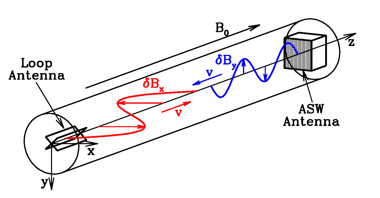
Figure 1: (Color online) Schematic of the experimental setup for the Alfvén wave turbulence experiment in the LaPD. The ASW antenna generates a small amplutude Alfvén wave (blue line) with a magnetic field polarized in the $\hat{\mathbf{y}}$ direction traveling down the mean magnetic field, $B_{0}$, and the Loop antenna generates a larger amplitude Alfvén wave (red line) with a magnetic field polarized in the $\hat{\mathbf{x}}$ direction traveling up the mean magnetic field. Howes et al. (2012)

The counterpropagating wave experiment requires two Alfvén wave antennas placed at either end of the plasma chamber, as shown in Fig. 1.Howes et al. (2012) The Iowa Arbitrary Spatial Waveform (ASW) antennaKletzing et al. (2010); Thuecks et al. (2009) was placed at $z$ = 15 m, where $z=0$ is at the cathode. This antenna, shown in Fig. 2, consists of a set of 48 vertical copper mesh grids of dimension 2.5 cm $\times$ 30.5 cm. Each element is driven by a separate amplifier which allows the current to be adjusted to a master signal with a multiplicative factor between -1 and 1. The plane of the mesh grid is oriented perpendicular to the axial magnetic field of the LaPD. By varying the amplitude of each grid element, we are able to create an arbitrary spatial waveform across the array in the $\hat{x}$ direction with effectively no variation in the $\hat{y}$ direction. Since Alfvén waves have $\delta B_{\parallel}=0$ and $\nabla\cdot\mathbf{B}=0$, then $\mathbf{k}_{\perp}\perp\delta\mathbf{B}_{\perp}$. Therefore, an Alfvén wave with a perpendicular wavevector $\mathbf{k}_{\perp}=k_{\perp}\hat{\mathbf{x}}$ has a perpendicular magnetic field fluctuation $\delta\mathbf{B}_{\perp}=\delta B_{\perp}\hat{\mathbf{y}}$ and, similarly, an Alfvén wave with a perpendicular wavevector $\mathbf{k}_{\perp}=k_{\perp}\hat{\mathbf{y}}$ has a perpendicular magnetic field fluctuation $\delta\mathbf{B}_{\perp}=\delta B_{\perp}\hat{\mathbf{x}}$ . For this experiment the ASW antenna generated an Alfvén wave (blue line in Fig. 1) with a sinusoidal waveform of frequency $f_{ASW}=$ 270 kHz or $\omega/\Omega_{i}\sim 0.22$, a parallel wavelength of $\lambda_{||_{ASW}}=6.5$ m, and a perpendicular wavevector of $k_{x}\rho_{s}\simeq\pm 0.18$, which propagates anti-parallel to the background magnetic field, $\mathbf{B}_{0}=B_{0}\hat{\mathbf{z}}$. Note that the ASW antenna will naturally produce both components of the perpendicular wave vector, $\pm k_{x}$.

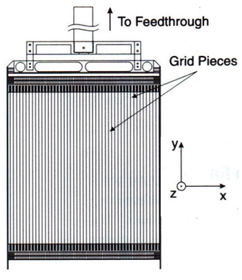
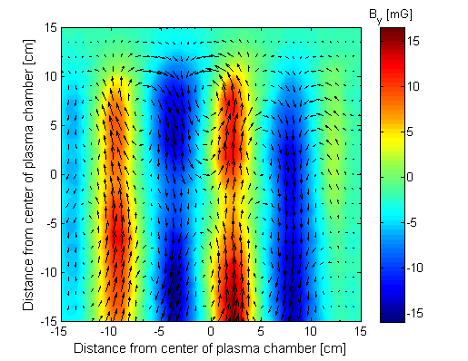
Figure 2: (Color online) Iowa ASW Antenna (a) diagram and (b) a colormap of the $\delta B_{y}$ component with vectors indicating the perpendicular component of the magnetic field measured in mG at $z=14$ m and $t$ = 8.3 ms after the beginning of the discharge.

The second antenna used in this experiment was the UCLA Loop antenna,Auerbach et al. (2011) which was placed at $z$ = 4.2 m. This antenna, shown in Fig. 3, consists of two overlapping rectangular loops of dimensions 21.5 cm $\times$ 29.5 cm, which are electrically isolated from each other. By orienting the loops perpendicular to each other and varying the relative phase of the driving signal on each loop, a large amplitude Alfvén wave can be produced with a magnetic field predominately in the $\hat{x}$ direction and a dominant perpendicular wavevecter in the $\hat{y}$ direction with $k_{y}\rho_{s}\simeq\pm 0.05$. For this experiment, the Loop antenna generated an Alfvén wave (red line in Fig. 1) with a sinusoidal waveform of frequency $f_{Loop}=$ 60 kHz, $\omega/\Omega_{i}\sim 0.05$, and a parallel wavelength of $\lambda_{||_{Loop}}=29.2$ m, which propagates parallel to $\mathbf{B}_{0}$ .

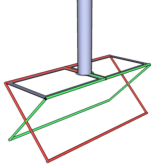
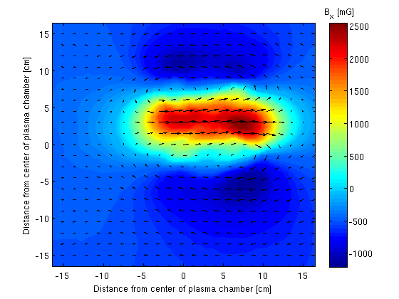
Figure 3: (Color online) UCLA Loop Antenna (a) diagram and (b) a colormap of the $\delta B_{x}$ component with vectors indicating the perpendicular component of the magnetic field measured in mG at $z=6.4$ m and $t$ = 8.2 ms after the beginning of the discharge. The offset in the data for the UCLA Loop antenna was due to a slight biasing issue with the Els$\ddot{\mbox{a}}$sser probes.

The perpedicular components of the magnetic field were measured using two Els$\ddot{\mbox{a}}$sser probes Drake et al. (2011) placed at $z$ = 6.4 m and $z$ = 14 m. These probes employ two B-dot coils constructed with forty 1.6 mm diameter loops of magnetic wire and oriented such that one is in the $\hat{x}$ plane and one is in the $\hat{y}$ plane. Measurements were performed over a 30 cm square region, centered on the machine axis, on a grid of locations separated by $\Delta$ = 0.75 cm. Using an ensemble of plasma discharges, time series with a sample frequency of 25 MHz (temporal resolution $\Delta t=0.04$ $\mu$s), data were collected at each of the spatial locations in turn with a specified starting time during the shot. Since the shot to shot variation in the LaPD is modest, averaging over 10 shots per spatial position for the ASW antenna Alfvén wave was sufficient to achieve a RMS noise level of $\sim$ 0.25 mG. The signal to noise is subsequently greatly enhanced by a spatial Fourier transform because we launch and detect waves that are nearly planar.

III.2 Experimental Procedure

The procedure for measuring the magnetic field fluctuations of the two counterpropagating waves follows. At $t$ = 8.0 ms, where $t$ = 0 s is at the start of the plasma discharge, the Loop antenna launches a wavepacket consisting of 30 wave periods which lasts for around 0.50 ms. At $t$ = 8.25 ms, the ASW antenna launches a wavepacket consisting of 20 wave periods (duration of 0.074 ms). Since the Loop antenna launches waves in both directions, that is towards the ASW antenna and towards the cathode, this time delay allows for ample time for the combined direct and reflected waves to reach a steady state before the ASW antenna launches its wave. Perpendicular magnetic field fluctuations are recorded before, during, and after the Loop antenna launches the large amplitude Alfvén wave. This procedure allows us to measure not only the entire interval when both antennas are turned on, but also the background noise in the plasma. This experiment was repeated five times with identical timings. Table 1 shows a summary of the five trials with the levels (max, half, and zero) indicating the amplitude of the magnetic field of each antenna.

Table 1: Summary of the five experimental trials.

Trial	ASW Amplitude	Loop Amplitude
1	maximum	maximum
2	maximum	zero
3	zero	maximum
4	maximum	half
5	half	maximum

The measured perpendicular magnetic field fluctuations produced by the ASW Alfvén waves in trial 2 and the Loop antenna waves in trial 3 are shown in Figs. 2 and 3, respectively. The colormaps in the figures include a linear interpolation to fill the locations in the plot between the actual measurements. Since the Els$\ddot{\mbox{a}}$sser probe employs a B-dot coil to measure the magnetic field, the measured signals are integrated in time in order to determine $\delta\mathbf{B_{\perp}}$. The colormaps show $\delta B_{y}(x,y,t)$ for the ASW antenna at $t=8.3$ ms and $\delta B_{x}(x,y,t)$ for the Loop antenna at $t=8.2$ ms. The vectors in each figure indicate the total vector $\delta\mathbf{B_{\perp}}$. The wave generated by ASW antenna has a typical amplitude of 30 mG in $\delta B_{y}(x,y,t)$ with almost no $\delta B_{x}(x,y,t)$ contribution, which indicates that the antenna produces a signal with a nearly pure $k_{x}$ perpendicular wavevector. On the other hand, the wave produced by the Loop antenna has a dominant $\delta B_{x}(x,y,t)$ component with a peak-to peak value of around 3500 mG and a small, but not insignifcant, $\delta B_{y}(x,y,t)$ component, $\sim$ 400 mG. The offset in the data for the UCLA Loop antenna is due to a slight biasing issue with the Els$\ddot{\mbox{a}}$sser probes.

IV Analysis of Experimental Measurements

One simple way of picturing the nonlinear interaction between the counterpropagating Alfvén waves in this experiment is as follows. The large-amplitude Loop antenna Alfvén wave generates a magnetic shear in the axial magnetic field which oscillates at the Loop antenna wave frequency, $f_{Loop}=60$ kHz. The nonlinear interaction is equivalent to the distortion of the ASW Alfvén wave as it propagates along this sheared magnetic field. The distorted ASW Alfvén wave is simply a linear combination of the initial ASW Alfvén wave and a nonlinearly generated daughter Alfvén wave. It is the primary goal of this experiment to measure and identify definitively this daughter Alfvén wave.

The daughter Alfvén wave measured at the Els$\ddot{\mbox{a}}$sser probe is generated by the nonlinear interaction that occurs only over the interaction region between the ASW antenna and the Els$\ddot{\mbox{a}}$sser probe, a length of $\Delta z=8.6$ m, see Fig. 2 in Paper III.Howes et al. (2013) Since $v_{A}=1.75\times 10^{8}$ cm/s, the time in which the two counterpropagating Alfvén waves may interact nonlinearly is $\Delta t=\Delta z/v_{A}=4.9\ \mu$s, less than $1/3$ the Loop antenna wave period, $T_{Loop}=16.7\ \mu$s. Over the time of the nonlinear interaction, the ASW Alfvén wave interacts with only a fraction of the wavelength of the Loop Alfvén wave. The resulting counterpropagating Alfvén wave signal experienced by the ASW Alfvén wave therefore has an effective $k_{\parallel}=0$ component as shown in Fig. 3 of Paper III. The nonlinear daughter wave generated by the $k_{\parallel}=0$ component of the Loop Alfvén wave and the ASW Alfvén wave is predicted theoretically to have the following properties:

1. The spatial location of the nonlinear daughter wave should correspond to the position that can be predicted by the nonlinear term in Els$\ddot{\mbox{a}}$sser form of the incompressible MHD equations.

2. The frequency band of the daughter wave will be the centered on the frequency of the ASW antenna wave signal, i.e. $f_{D}=f_{ASW}$, or $k_{\parallel_{D}}=k_{\parallel_{ASW}}$.

3. The nonlinear three-wave interaction should satisfy $\mathbf{k}_{\perp_{D}}=\mathbf{k}_{\perp_{ASW}}+\mathbf{k}_{\perp_{Loop}}$.

4. The amplitude of the nonlinear daughter wave should agree with theoretical predictions.

As discussed previously, the Els$\ddot{\mbox{a}}$sser probe employs a B-dot coil to measure the $\delta\dot{B}_{x}(x,y,t)$ and $\delta\dot{B}_{y}(x,y,t)$ of a fluctuating magnetic field. From the theory we predict that the daughter wave will have the same frequency as the Alfvén wave produced by the ASW antenna, $f_{ASW}=270$ kHz. Since the ASW antenna produces a wave almost exclusively in the $\hat{y}$ direction and $f_{ASW}$ falls between the third and fourth harmonic of the Loop antenna signal, the only signal measured on $\delta\dot{B}_{x}(x,y,t)$ component at $f_{ASW}$ should be the daughter wave signal. Therefore, we first subtract the $\delta\dot{B}_{x_{Loop}}$, data from trial 3, from the data in which both antennas are on and measured at $z=6.4$ m, trials 1, 4, or 5. This effectively eliminates the linear contribution from the large amplitude Alfvén wave produced by the Loop antenna. Next, we integrate this result to obtain $\delta B_{x_{D}}(x,y,t)$. From these results we select a time interval in which both waves are measured, 8.25 ms $\leq t\leq$ 8.32 ms, and Fourier transform this interval in time to obtain $\delta B_{x_{D}}(x,y,f)$. Since we expect the daughter wave to have a frequency corresponding to that of the ASW antenna, $f$ = 270 kHz, a bandpass filter is applied to this data to eliminate the frequencies below $f$ = 170 kHz and above $f$ = 370 kHz. Finally, the resulting data sequence is inverse Fourier transfromed back into the time domain, $\delta B_{x_{D}}(x,y,t)$. The results of this analysis are shown at $t$ = 8.30 ms in Fig. 4.

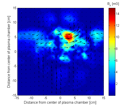
Figure 4: (Color online) Colormap of the $\delta B_{x}$ component of the daughter wave with vectors indicating the perpendicular component of the magnetic field at $t$ = 8.30 ms.

IV.1 Spatial Localization

We can use the nonlinear term in Eq. (1) to predict the position where the nonlinear daughter wave will appear in the experiment. This nonlinear term describing the distortion of the ASW Alfvén wave by the Loop Alfvén wave is given by $\mathbf{z}^{-}_{Loop}\cdot\nabla\mathbf{z}^{+}_{ASW}$. The eigenfunction for an Alfvén wave traveling up the magnetic field determines that $\mathbf{v}_{\perp}=-\delta\mathbf{B}_{\perp}/\sqrt{\mu_{0}\rho_{0}}$, so the Els$\ddot{\mbox{a}}$sser field for the Loop Alfvén wave can be expressed simply in terms of its magnetic perturbation $\mathbf{z}^{-}_{Loop}=-2\delta\mathbf{B}_{\perp Loop}/\sqrt{\mu_{0}\rho_{0}}$. Similarly, the eigenfunction for an Alfvén wave traveling down the magnetic field is given by $\mathbf{v}_{\perp}=\delta\mathbf{B}_{\perp}/\sqrt{\mu_{0}\rho_{0}}$, so that $\mathbf{z}^{+}_{ASW}=2\delta\mathbf{B}_{\perp ASW}/\sqrt{\mu_{0}\rho_{0}}$. Note that this eigenfunction is correct not only in the MHD limit of strong collisionality and large scales, $k\rho_{s}\ll 1$, but also in the limit appropriate for the LaPD experiment of moderate collisionality and large scales.Schekochihin et al. (2009); Howes and Nielson (2013); Howes, Nielson, and Dorland (2013); Howes et al. (2013)

Since the variation of the magnetic field of the ASW Alfvén wave is only in the $x$-direction, this nonlinear term simplifies to

$$\delta B_{xLoop}\frac{\partial\delta B_{yASW}}{\partial x},$$ (4)

where we have dropped constant factors. The daughter Alfvén wave is generated by this term,Note (1) which predicts that the magnetic field for the daughter Alfvén wave will be maximum at the spatial position where the Loop antenna’s magnetic field, $\delta B_{xLoop}$, is largest and the gradient of the ASW antenna’s magnetic field, $\partial/\partial x(\delta B_{yASW})$, is largest. We can employ the magnetic field patterns from the single-antenna runs, shown in Figs. 2 and 3, to compute this term to predict the position of the maximum amplitude of the nonlinearly generated daughter Alfvén wave, as shown in Fig. 5. The result of this very simple prediction agrees well with the measurement of the daughter wave, shown in Fig. 4, which has a maximum value of 14 mG at position $\delta B_{x}$ ($x$ = 3 cm, $y$ = 5 cm). This agreement corresponds to the first of our listed predictions for the properties of the daughter Alfvén wave generated by the nonlinear interaction between the two counterpropagating Alfvén waves launched in the experiment.

Figure 5: (Color online) Colormap of the predicted coupling between the Loop and ASW antennas. The dark spot at ($x$ = 3 cm, $y$ = 7 cm) indicates the position in the plane where the nonlinear effect is predicted to have the largest amplitude.

IV.2 Frequency selection

The second property predicted for the daughter wave is that the frequency of the daughter wave is the same as the frequency of the ASW antenna wave, $f_{D}=f_{ASW}$ or equivalently $k_{\parallel_{D}}=k_{\parallel_{ASW}}$. Since the ASW wave antenna has a magnetic field predominantly in the $\hat{y}$ direction, one way to distinguish the daughter wave from the ASW wave is to look at the $\delta B_{x}$ component of the waves in the frequency domain. Because the daughter wave is a nonlinear effect, the amplitude should vary as the product of the primary wave amplitudes, as shown by Eq. 36 in Paper I.Howes and Nielson (2013) Thus, if the amplitude of either antenna signal is reduced by half, the amplitude of the daughter wave should also be reduced by half. If the signal at 270 kHz was related to one of the primary waves, this would not occur. Thus by observing what occurs when the Loop and ASW antenna amplitudes are individually decreased by half, we can look for the presence of a nonlineraly generated daughter wave. In Fig. 6, we show the daughter wave signal (blue) at 270 kHz when both antennas are at full power and at position $\delta B_{x}$ ($x$ = 3 cm, $y$ = 5 cm, $f$), which is where the maximum of the nonlinear effect occurred as shown in Fig. 4. Fig. 6 also shows, at the same axial position, results for trial 4, when the Loop antenna signal is turned down to half power and the ASW antenna is kept at full power (red), and trial 5, when the ASW antenna is turned to half power and the Loop antenna is at full (green). These results clearly demonstrate that the daughter wave signal decreases by the same amount ($\sim$ 40%) when either of the antenna amplitudes is decreased. Note that when the two antennas are at full power, the antenna coupling into the plasma is starting to saturate, and thus the response is not perfectly linear.

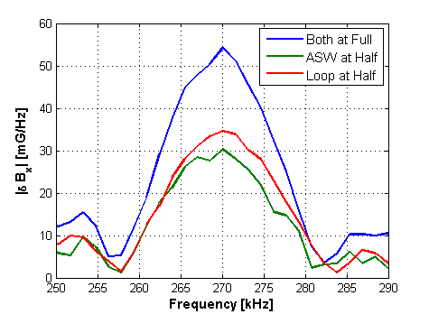
Figure 6: (Color online) Plot of the amplitude of the daughter wave in frequency where the maximum of the nonlinear signal occurs, $\delta B_{x}$ ($x$ = 3 cm, $y$ = 5 cm, $f$). We show the results for when both antennas are at full power (blue), the ASW antenna is at half power and the Loop antenna is at full power (green), and when the Loop antenna is at half and the ASW antenna is at full (red).

IV.3 Wave number selection

The third prediction for the daughter wave signal is that $\mathbf{k}_{\perp_{D}}=\mathbf{k}_{\perp_{ASW}}+\mathbf{k}_{\perp_{Loop}}$. To obtain the spatial Fourier transform in the perpendicular plane for each antenna signal and the daughter wave signal, we Fourier transform the data shown in Figs. 2, 3, and 4 in both the $\hat{x}$ and $\hat{y}$ directions, which yields $\delta\mathbf{B}_{x}(k_{x},k_{y},t)$ for the Loop antenna signal and $\delta\mathbf{B}_{y}(k_{x},k_{y},t)$ for the ASW antenna. We present these results in Fig. 7 at $t$ = 8.30 ms.Howes et al. (2012) In Fig. 7 (b) we show the two-dimensional Fourier transform of the Loop antenna data in Fig. 3, which shows that the the $\delta B_{x}$ component of the Loop antenna has a perpendicular wavevector of $k_{y}\rho_{s}=\pm 0.06$. Fig. 7 (c) shows the Fourier transform of the $\delta B_{y}(k_{x},k_{y},t)$ of the ASW antenna signal in Fig. 2, clearly indicating that the perpendicular wavevector for the $\delta B_{y}$ component of the ASW antenna is $k_{x}\rho_{s}=\pm 0.16$. This value is close to the expected value of $k_{x}\rho_{s}\simeq\pm 0.2$ (see Sec. III A). The small discrpency in these two values is because the density profile is not perfectly flat, which can produce a small shift in the $k_{\perp}$ of an Alfvén wave. The resulting daughter wave, $\delta B_{x}(k_{x},k_{y},t)$, is shown in Fig. 7 (a), which was taken from the Fourier transform of Fig. 4. We can clearly see that the daughter wave signal is a sum of the ASW and Loop antenna wavenumbers, $\mathbf{k}_{\perp_{D}}=+(\mathbf{k}_{\perp_{ASW}}\pm\mathbf{k}_{\perp_{Loop}})$ and $\mathbf{k}_{\perp_{D}}=-(\mathbf{k}_{\perp_{ASW}}\pm\mathbf{k}_{\perp_{Loop}})$. A diagram of the three wave interaction process is shown in panel (d). Here $\mathbf{k}_{1}$, in blue, indicates the perpendicular wavevector contributions of the $\delta B_{y}$ of the ASW antenna. $\mathbf{k}_{2}$, shown in red, is the perpendicular wavevector produced by the $\delta B_{x}$ of the Loop antenna. Note that both antennas produce a pair of wavevectors with $\pm\mathbf{k}_{1,2}$. The daughter wave should be a vector sum of the type, $\mathbf{k}_{3}=\mathbf{k}_{1}+\mathbf{k}_{2}$. The bullseyes indicate the predicted values for the daughter wave. These predictions align well with experimental results in panel (a).

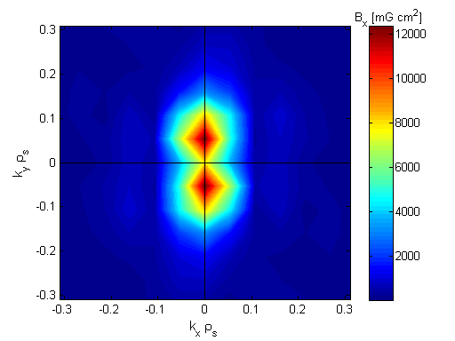
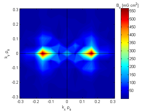
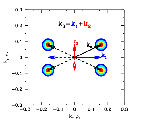
Figure 7: (Color online) Contour plots of the two-dimensional Fourier power spectrum of the (a) $\delta B_{x}$ component of the daughter signal, (b) the $\delta B_{x}$ component of the Loop signal, (c) the $\delta B_{y}$ component of the ASW antenna signal, and (d) is the diagram of the perpendicular wavevectors for the Loop antenna (red line) and the ASW antenna (blue line). The daughter wave should be a vector sum of the type, $\mathbf{k}_{3}=\mathbf{k}_{1}+\mathbf{k}_{2}$. The bullseyes indicate the predicted values for the daughter wave. Howes et al. (2012)

IV.4 Amplitude of Daughter wave

A final line of evidence that the signal measured in the experiment is the nonlinearly generated daughter Alfvén wave is to compare the measured magnitude of the signal to the theoretical prediction. An asymptotic solution for the nonlinear evolution of the interaction between counterpropagating Alfvén waves has been derived in Paper I Howes and Nielson (2013) of this series. The second-order nonlinear solution for two counterpropagating Alfvén waves with equal $k_{\perp}$ and $k_{\parallel}$ is given by Eq. 36 in Paper I. Therefore, we estimate that the nonlinear daughter wave in our case will have an amplitude

$$\frac{|\mathbf{B}_{\perp 2}|}{B_{0}}=\frac{z_{+}z_{-}}{16v_{A}^{2}}\frac{k_{\perp}}{k_{\parallel}}$$ (5)

Using the eigenfunction for an Alfvén wave, ${u_{\perp}}/{v_{A}}=\pm{B_{\perp}}/{B_{0}}$, the magnitude of the Els$\ddot{\mbox{a}}$sser variables $z^{\pm}$ are related to the magnetic field perturbation by $z_{\pm}/v_{A}=2{B}^{\pm}_{\perp}/B_{0}$.

We can therefore express the nonlinear daughter wave magnetic amplitude $\delta{B}_{\perp D}$ in terms of the loop wave amplitude $\delta{B}_{\perp L}$ and the ASW wave amplitude $\delta{B}_{\perp A}$,

$$\frac{\delta B_{\perp D}}{B_{0}}=\frac{1}{4}\frac{{\delta B}_{\perp L}}{B_{0}}\frac{{\delta B}_{\perp A}}{B_{0}}\frac{k_{\perp}}{k_{\parallel}}$$ (6)

The normalized amplitudes in this expression correspond to the amplitudes of the Fourier coefficients in Fig. 7, corresponding to $B_{\perp D}=16$ mG cm², $B_{\perp L}=12000$ mG cm², and $B_{\perp A}=550$ mG cm². These values must be normalized to an appropriate value of $B_{0}$, so we use the ratio of the maximum Loop antenna magnetic field magnitude from Fig. 3 divided by the axial magnetic field to estimate the normalized value for $B_{\perp L}/B_{0}=1.5\mbox{G}/800\mbox{ G}=1.9\times 10^{-3}$. Using this value, we can estimate the other normalized values as $B_{\perp A}/B_{0}=8.7\times 10^{-5}$ and $B_{\perp D}/B_{0}=2.5\times 10^{-6}$. To compute the ratio $k_{\perp}/k_{\parallel}$ for the ASW Alfvén wave, we take $\lambda_{\parallel}=v_{A}/f=1.75\times 10^{8}\mbox{ cm s}^{-1}/2.7\times 10^{5}\mbox{ Hz}=648$ cm, and $\lambda_{\perp}=10.16$ cm. This leads $k_{\perp}/k_{\parallel}=\lambda_{\parallel}/\lambda_{\perp}=64$.

Substituting these values into Eq. 36 of Paper I, we obtain a predicted normalized amplitude of $B_{\perp D}/B_{0}=2.6\times 10^{-6}$, in striking agreement with the measured normalized value of $B_{\perp D}/B_{0}=2.5\times 10^{-6}$. This calculation indicates that the amplitude of the nonlinearly generated wave agrees extremely well with the predictions from analytical theory.

V Conclusions

In this paper we present the first experimental verification of the properties of the nonlinear interaction between two counterpropagating Alfvén waves as derived from incompressible MHD. We have confirmed that the nonlinear interaction between the Loop antenna and the ASW antenna is well described by the nonlinear term in the Els$\ddot{\mbox{a}}$sser equation, Eq. (1). In this case, the maximum for the nonlinear signal will appear at the location where both the magnitude of the Loop antenna and the gradient of the ASW antenna are largest. This was clearly evident in the comparison of the measured spatial plot of the daughter wave, Fig. 4, and the colormap of the predicted location, Fig. 5. From Fig. 6, we saw that the daughter wave has a peak at the expected frequency of 270 kHz, which corresponds to the frequency of the ASW antenna wave signal. In Fig. 7, we observed that the perpendicular structure of the daughter wave is dominated by four wavevectors corresponding to $\mathbf{k}_{\perp_{D}}=\mathbf{k}_{\perp_{ASW}}+\mathbf{k}_{\perp_{Loop}}$. Since the measured daughter wave signal satisfies the theoretical predictions, we conclude that we have measured the nonlinear interaction between two counterpropagating Alfvén waves. This evidence supports the use of such idealized models, as discussed in Paper I,Howes and Nielson (2013) for weakly collisional plasmas which are relevant to various space and astrophysical plasma environments. It is important to note that this procedure, of subtracting the parent wave signals and bandpass filtering the data, is not required to see the nonlinear daughter wave signal since the three waves are in different locations in the $k$-plane and vector orientation of $\delta B_{\perp}$ in the plane is different. Although the parent Alfvén wave signals are much greater in magnitude then the daughter wave signals, the contributions of the parent waves to the daughter signal at the particular $k$-plane location, vector orientation, and frequency is very modest and well resolved given the RMS noise level of $\sim 0.25$ mG.