Shortcuts to adiabaticity by counter-diabatic driving

Abstract

The evolution of a system induced by counter-diabatic driving mimics the adiabatic dynamics without the requirement of slow driving. Engineering it involves diagonalizing the instantaneous Hamiltonian of the system and results in the need of auxiliary non-local interactions for matter-waves. Here experimentally realizable driving protocols are found for a large class of single-particle, many-body, and non-linear systems without demanding the spectral properties as an input. The method is applied to the fast decompression of Bose-Einstein condensates in different trapping potentials.

The development of new methods to induce adiabatic dynamics is key to the progress of quantum technologies CZ12 . The emergent field of shortcuts to adiabaticity aims at designing non-adiabatic protocols which reproduce the same target state that would result in a strictly adiabatic dynamics. In the last few years, a great deal of attention has been devoted to this goal, and theoretical efforts DR03 ; Berry09 ; MN10 ; Chen10 ; Muga10 ; Stefanatos10 ; Hoffmann11 ; delcampo11b ; RC11 ; Torrontegui11 ; DB12 ; Stefanatos13 have been accompanied by a remarkable experimental progress Schaff1 ; Schaff2 ; ions1 ; ions2 ; expCD1 ; expCD2 . Among the variety of techniques developed, counter-diabatic driving (CD) DR03 , also known as transitionless quantum driving Berry09 , stands out as a technique to control and engineer the fast evolution of a system mimicking adiabaticity. Indeed, it is tantamount to induce a “fast motion video of the adiabatic dynamics”. Consider a time-dependent Hamiltonian $\hat{H}(t)$ with instantaneous eigenvalues $\{\varepsilon_{n}(t)\}$ and eigenstates $\{|n(t)\rangle\}$. Whenever $\hat{H}(t)$ is slowly-varying, the dynamics for the $n$-th eigenstate in the adiabatic approximation reads

$$|\psi_{n}(t)\rangle=e^{-i\int^{t}dt^{\prime}\varepsilon_{n}(t^{\prime})}e^{-\int^{t}dt^{\prime}\langle n|\partial_{t^{\prime}}n\rangle}|n(t)\rangle,$$ (1)

which includes both the dynamical phase and the geometric phase. The central goal of CD is to find a Hamiltonian $\hat{H}_{\rm CD}$ for which the adiabatic approximation to $\hat{H}$ becomes the exact solution of the time-dependent Schrödinger equation for $\hat{H}_{\rm CD}$. Direct construction of the time evolution operator

$$\hat{U}_{\rm CD}(t,t^{\prime}=0)=\sum_{n}|\psi_{n}(t)\rangle\langle n(0)|,$$ (2)

allows one to derive the form of $\hat{H}_{\rm CD}$,

$$\hat{H}_{\rm CD} = i\hbar\hat{U}_{\rm CD}(t)^{{\dagger}}\partial_{t}\hat{U}_{\rm CD}(t)=\hat{H}+\hat{H}_{1},$$ (3)

$$\hat{H}_{1} = i\hbar\sum_{n}(|\partial_{t}n\rangle\langle n|-\langle n|\partial_{t}n\rangle|n\rangle\langle n|).$$ (4)

It follows that $\hat{H}_{1}$ is the auxiliary term required to implement this type of shortcut. Note that other choices of the phase in Eq. (1) are possible. An example of relevance is the dynamics $|\phi_{n}(t)\rangle=e^{-i\int^{t}dt^{\prime}\varepsilon_{n}(t^{\prime})}|n(t)\rangle$, associated with the unitary time-evolution operator $\hat{U}_{\rm CD}^{\prime}(t,t^{\prime}=0)=\sum_{n}|\phi_{n}(t)\rangle\langle n(0)|$, and generated by the counter-diabatic Hamiltonian

$$\hat{H}_{\rm CD}^{\prime}=\hat{H}+\hat{H}_{1}^{\prime}=\hat{H}+i\hbar\sum_{n}|\partial_{t}n\rangle\langle n|.$$ (5)

The experimental demonstration of the CD technique has recently been reported in effective two-level systems arising in a Bose-Einstein condensate trapped in an optical lattice expCD1 as well as in an electron spin of a single nitrogen-vacancy center expCD2 . It can be extended to many-body spin systems undergoing a quantum phase transition, at the cost of implementing $n$-body interactions DRZ12 , which are necessary to suppress the universal formation of excitations and defects QKZM . Nonetheless, the application of this technique to systems with continuous variables such as matter waves seems to be hindered by the non-local nature of the counter-diabatic Hamiltonian $\hat{H}_{1}^{\prime}$. Jarzynski has recently shown that for a quantum piston with one degree of freedom $q$ and for any power-law trap of the form $V(q)=\alpha|q|^{b}$ Jarzynski13 , the counter-diabatic term is

$$\hat{H}_{1}^{\prime}\propto(qp+pq),$$ (6)

where $p$ is the momentum operator canonically conjugated to $q$. This is in agreement with previous calculations for a time-dependent harmonic trap ($b=2$) Muga10b . The implementation of this non-local Hamiltonian in trapped ions and ultracold atoms by optical means seems challenging. Another important limitation of the CD technique is that it demands knowledge of the spectral properties of the Hamiltonian $\hat{H}(t)$, that is, of the instantaneous eigenvalues and eigenstates as a function of $t$. As a result, the CD is unsuited for systems obeying an effectively-nonlinear dynamics that often arises in mean-field/Hartree-Fock approximations, as it is the case for Bose-Einstein condensates described by the Gross-Pitaevskii equation and its variants Ueda . Further, direct computation of $\hat{H}_{1}$ ($\hat{H}_{1}^{\prime}$) in other many-body systems is either impossible due to the lack of knowledge of the spectral properties, or would constitute a daunting task as in the case of exactly solvable models, e.g. by Bethe ansatz in homogeneous potentials.

In this letter, all these difficulties are overcome by reformulating counter-diabatic driving in terms of scaling laws. Specifically, i) a counter-diabatic driving protocol is derived for single-particle, many-body, and non-linear systems undergoing self-similar dynamics in a variety of trapping potentials, ii) the requirement to diagoanalize the Hamiltonian of the system $\hat{H}(t)$ is completely removed, iii ) it is shown that while the requirement of a non-local counter-diabatic term of the form $\hat{H}_{1}^{\prime}\propto(qp+pq)$ is a common feature in matter waves (such as trapped ions, ultracold gases and other strongly-correlated quantum fluids), it is possible to find an alternative representation of $\hat{H}_{\rm CD}$ associated with an auxiliary term $\hat{H}_{1}$ which is local and experimentally realizable with well-established techniques.

Let us consider the broad family of many-body systems, described by the Hamiltonian

$$\hat{\mathcal{H}} = \!\sum_{i=1}^{N}\!\Big{[}-\frac{\hbar^{2}}{2m}\Delta_{{\rm\bf q}_{i}}+\frac{1}{2}m\omega^{2}(t){\rm\bf q}_{i}^{2}+{\rm U}({\rm\bf q}_{i},t)\!\Big{]}\!$$ (7)

$$+\epsilon(t)\sum_{i<j}V({\rm\bf q}_{i}-{\rm\bf q}_{j}),$$

where ${{\rm\bf q}_{i}}\in\mathbb{R}^{D}$ ($D$ denoting the effective dimension of the system), $\Delta_{{\rm\bf q}_{i}}$ is the Laplace operator, and ${\rm U}({\rm\bf q}_{i},t)$ represents an external trap whose time-dependence is of the form ${\rm U}({\rm\bf q},t)={\rm U}({\rm\bf q}/\gamma,0)/\gamma^{2}$, $\gamma=\gamma(t)$ being a function of time. The two-body interaction potential obeys

$${\rm V}(\lambda{\rm\bf q})=\lambda^{-\alpha}{\rm V}({\rm\bf q}),$$ (8)

which among other relevant examples includes the pseudo-potential describing s-wave scattering in ultracold gases, for which $\alpha=D$. Without loss of generality, we choose the dimensionless time-dependent coupling constant $\epsilon(t)$ to satisfy $\epsilon(0)=1$. We further consider a stationary state at $t=0$, $\Phi(t)=\Phi({\rm\bf q}_{1},\dots,{\rm\bf q}_{N};t)$, with chemical potential $\mu$, i.e., $\hat{\mathcal{H}}\Phi=\mu\Phi$ (an assumption we shall remove below).

We begin by pointing out that for a single-particle harmonic oscillator of a single-degree of freedom, two-eigenstates $|n(\omega_{1})\rangle$ and $|n(\omega_{2})\rangle$ corresponding to the $n$-th mode of two different traps of frequencies $\omega_{1}$ and $\omega_{2}$ are related by the scaling transformation

$$\langle q|n(\omega_{2})\rangle=\gamma_{12}^{-1/2}\langle q/\gamma_{12}|n(\omega_{1})\rangle,$$ (9)

where $\gamma_{12}=[\omega_{1}/\omega_{2}]^{\frac{1}{2}}$ plays the role of a (adiabatic) scaling factor. Under such type of scaling, the dynamics is self-similar in real-space. An analogous scaling law, is fulfilled in the quantum piston and power-law traps recently discussed by Jarzynski Jarzynski13 , and can be extended to many other systems GBD10 . Indeed, exploitation of scaling laws has proved useful in engineering a type of shortcut to adiabatic which does not drive the dynamics through the adiabatic manifold of $\hat{\mathcal{H}}(t)$ delcampo11b ; DB12 . Motivated by this observation, we consider the time-evolution $\Phi(t)$ of the initial state to be described by the simple scaling

$$\Phi(t)=\gamma^{-\frac{ND}{2}}e^{-i\mu\tau(t)/\hbar}\Phi\Big{[}\frac{{\rm\bf q}_{1}}{\gamma(t)},\dots,\frac{{\rm\bf q}_{N}}{\gamma(t)};0\Big{]},$$ (10)

where the prefactor accounts for the correct normalization and $\tau(t)$ is a function of time soon to be determined. We note that we will not necessitate knowledge of the precise form of $\Phi(t=0)$. Direct substitution into the many-body Schrödinger equation for $\hat{\mathcal{H}}$ shows that the ansatz Eq. (10) is actually the exact time-dependent solution of the counter-diabatic Hamiltonian $\hat{\mathcal{H}}^{\prime}_{\rm CD}$, with

$$\gamma^{2}\hat{\mathcal{H}}^{\prime}_{\rm CD} = \!\sum_{i=1}^{N}\!\Big{[}-\frac{\hbar^{2}}{2m}\Delta_{{\rm\bf\sigma}_{i}}+\frac{1}{2}m\omega^{2}(t)\gamma^{4}{\rm\bf\sigma}_{i}^{2}+{\rm U}({\rm\bf\sigma}_{i},0)$$

$$-i\frac{\hbar\partial_{\tau}\gamma}{2\gamma}({\rm\bf\sigma}_{i}\partial_{{\rm\bf\sigma}_{i}}+\partial_{{\rm\bf\sigma}_{i}}{\rm\bf\sigma}_{i})\Big{]}\!+\epsilon\gamma^{2-\alpha}\sum_{i<j}V({\rm\bf\sigma}_{i}-{\rm\bf\sigma}_{j}),$$

where the scaled spatial coordinate and time variables read

$${\rm\bf\sigma}_{i}={\rm\bf q}_{i}/\gamma,\qquad\tau=\int^{t}\gamma^{-2}(t^{\prime})dt^{\prime}.$$ (12)

One can choose a suitable time-dependence of $\omega^{2}(t)$ and $\epsilon(t)$ to render $\gamma^{2}\hat{\mathcal{H}}^{\prime}_{\rm CD}$ time-independent, and to reduce it to its form at $t=0$, when $\omega(0)=\omega_{0}$ and $\epsilon(0)=1$. This requirement leads to the the consistency conditions

$$\gamma(t) = \bigg{[}\frac{\omega_{0}}{\omega(t)}\bigg{]}^{\frac{1}{2}},$$ (13)

$$\epsilon(t) = \bigg{[}\frac{\omega_{0}}{\omega(t)}\bigg{]}^{\frac{\alpha-2}{2}}.$$ (14)

Under this choice, $\Phi(0)$ remains a stationary solution of $\gamma^{2}\hat{\mathcal{H}}^{\prime}_{\rm CD}$ with chemical potential $\mu$. Similarly, an initial nonstationary state follows a trivial dynamics in the scaled variables note . The first consistency equation can be considered the definition of the adiabatic scaling factor in a self-similar dynamics. It agrees with the well-known result of the single-particle harmonic oscillator. The second condition implies that for a self-similar dynamics to occur in an interacting-many-body system it might be necessary to change along the process the amplitude of the interactions. In ultracold gases, this can be achieved by means of a Feschbach resonance or a modulation of the transverse confinement. However, for moderate changes of the scaling factors, this condition can be dropped -one can set $\epsilon(t)=1$- and the dynamics is self-similar to a high accuracy DB12 . In addition, certain systems satisfy the condition $\alpha=2$ so that $\epsilon(t)=1$ is fulfilled exactly, and no interaction tuning is required. This is the case of a two-dimensional Bose gas, as a reflection of the Pitaevskii-Rosch symmetry PR97 . The same is true for the family of Tonks-Girardeau gases with effectively infinite strength of interactions GNO04 , the Calogero-Sutherland model Sutherland98 , etc.

Provided that these equations are satisfied, the scaling ansatz (10) is an exact solution of the many-body time-dependent Schrödinger equation. This result provides a way to apply counter-diabatic driving to the broad family of systems described by Eq. (Shortcuts to adiabaticity by counter-diabatic driving) without the need to perform the explicit computation in (3). By doing so, it removes the requirement to diagonalize the Hamiltonian of the system of interest $\hat{H}(t)$, a feature particularly useful to design shortcuts to adiabaticity in interacting many-body systems. As we shall discuss below, it can be applied as well to non-linear equations of motion. Further, one can identify the auxiliary CD term

$$\hat{\mathcal{H}}_{1}^{\prime}=-i\frac{\hbar\dot{\gamma}}{2\gamma}\sum_{i=1}^{N}({\rm\bf q}_{i}\partial_{{\rm\bf q}_{i}}+\partial_{{\rm\bf q}_{i}}{\rm\bf q}_{i}),$$ (15)

which is needed to drive an arbitrary self-similar dynamics of matter-waves through the adiabatic manifold $\hat{\mathcal{H}}$ (dots denote derivatives with respect to time $t$ throughout the text).

A non-local term like $\hat{\mathcal{H}}_{1}^{\prime}$ is present in generalized harmonic oscillators, and following bookinv , we next find an alternative representation of $\hat{\mathcal{H}}_{\rm CD}^{\prime}$ in which this term is absent. In order to do so, we consider the $N$-body canonical transformation,

$$\mathcal{U} = \prod_{i=1}^{N}\exp\left(\frac{im\dot{\gamma}}{2\hbar\gamma}{\rm\bf q}_{i}^{2}\right)$$ (16)

whose action on ${\rm\bf q}_{i}$, ${\rm\bf p}_{i}$, and $\hat{\mathcal{H}}_{\rm CD}^{\prime}$ is as follows,

$${\rm\bf q}_{i} \rightarrow \mathcal{U}{\rm\bf q}_{i}\mathcal{U}^{{\dagger}}={\rm\bf q}_{i},$$ (17)

$${\rm\bf p}_{i} \rightarrow \mathcal{U}{\rm\bf p}_{i}\mathcal{U}^{{\dagger}}={\rm\bf p}_{i}-\frac{m\dot{\gamma}(t)}{\gamma(t)}{\rm\bf q}_{i},$$ (18)

$$\hat{\mathcal{H}}_{\rm CD}^{\prime} \rightarrow \hat{\mathcal{H}}_{\rm CD}(t)=\mathcal{U}\hat{\mathcal{H}}_{\rm CD}^{\prime}(t)\mathcal{U}^{{\dagger}}-i\hbar\mathcal{U}\partial_{t}\mathcal{U}^{{\dagger}}.$$ (19)

As a result of (18), the kinetic energy term in the Hamiltonian is modified, and upon expansion the non-local counter-diabatic term (15) is cancelled. The new representation $\hat{\mathcal{H}}_{\rm CD}(t)$ of the counter-diabatic Hamiltonian resembles that of the original Hamiltonian $\hat{\mathcal{H}}$,

$$\hat{\mathcal{H}}_{\rm CD} = \!\sum_{i=1}^{N}\!\Big{[}-\frac{\hbar^{2}}{2m}\Delta_{{\rm\bf q}_{i}}+\frac{1}{2}m\Omega^{2}(t){\rm\bf q}_{i}^{2}+U({\rm\bf q}_{i},t)\Big{]}\!$$ (20)

$$+\epsilon(t)\sum_{i<j}V({\rm\bf q}_{i}-{\rm\bf q}_{j}),$$

with the modified time-dependent (squared) frequency

$$\Omega^{2}(t) = \omega^{2}(t)-\frac{\ddot{\gamma}}{\gamma},$$ (21)

this is, the counter-diabatic driving reduces the trap frequency by a term proportional to the acceleration of the scaling factor, a result which resembles the outcome of the Duru transformation in transport problems Duru89 . For $\gamma(t)$ in (13), Eq. (21) reduces to

$$\Omega^{2}(t)=\omega^{2}(t)-\frac{3}{4}\bigg{[}\frac{\dot{\omega}(t)}{\omega(t)}\bigg{]}^{2}+\frac{1}{2}\frac{\ddot{\omega}(t)}{\omega(t)}.$$ (22)

Under this canonical transformation the time-evolution of the initial state, instead of being described by Eq. (10), is mapped to $\Phi(t)\rightarrow\Psi(t)=\mathcal{U}\Phi(t)$, with

$$\Psi({\rm\bf q}_{1},\dots,{\rm\bf q}_{N};t)=\exp\left(-i\frac{m\dot{\omega}(t)}{4\hbar\omega(t)}\sum_{i=1}^{N}{\rm\bf q}_{i}^{2}\right)\Phi(t),$$ (23)

that is, it acquires the Berry phase which vanishes only as $\dot{\omega}/\omega\rightarrow 0$ but is non-zero along a shortcut to adiabaticity assisted by CD.

Let us summarize the results above. To drive the dynamics of a given state of $\hat{\mathcal{H}}$ mimicking adiabaticity for the driving $\omega(t)$, it suffices to implement instead the counter-diabatic driving $\Omega(t)$ and to fulfill the consistency conditions Eqs. (13) and (14), which are still referred to the driving $\omega(t)$. It is worth pointing out that the frequency modulation in Eq. (22) was derived before in a different context, that of a single-particle time-dependent harmonic oscillator, as the consistency condition for a time-dependent Gaussian variational ansatz for the instantaneous ground state delcampo11 . CD for self-similar process is as well related to the inversion of the scaling laws for a time-dependent harmonic oscillator Chen10 , choosing $\gamma(t)$ according to Eq. (13) and promoting $\omega(t)\rightarrow\Omega(t)$ in the corresponding consistency equation (Ermakov equation).

A possible implementation of a shortcut to adiabaticity assisted by CD would be as follows. Consider the case in which we are interested in driving a transition from $|n(0)\rangle$ to $|n(t_{\rm F})\rangle$ in a time $t_{\rm F}$. The condition for the CD driving Hamiltonian to equal the system Hamiltonian $\hat{\mathcal{H}}_{\rm CD}(t)=\hat{\mathcal{H}}(t)$ at $t=\{0,t_{\rm F}\}$, leads to the boundary conditions

$$\omega(0) = \omega_{0},\dot{\omega}(0)=0,\ddot{\omega}(0)=0,$$

$$\omega(t_{\rm F}) = \omega_{F},\dot{\omega}(t_{\rm F})=0,\ddot{\omega}(t_{\rm F})=0,$$ (24)

which can be satisfied by an interpolating ansatz. Choosing it to be a polynomial $\omega(t)=\sum_{k=1}^{6}a_{k}(t/t_{\rm F})^{k-1}$ we find

$$\omega(t)=\omega_{0}+10\delta s^{3}-15\delta s^{4}+6\delta s^{5},$$ (25)

where $\delta=\omega_{\rm F}-\omega_{0}$ and $s=t/t_{\rm F}$ for short.

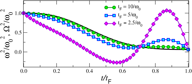
Figure 1: Shortcut to adiabaticity by counter-diabatic driving. The time-dependent frequency $\omega(t)$ (solid line) in Eq. (25) does not suffice to fulfill adiabaticity in a finite time $t_{\rm F}$. The necessary counter-diabatic driving of the trap frequency $\Omega(t)$ for a shortcut to an adiabatic expansion is given by Eq. (22) and is displayed here for three different values of $t_{\rm F}$ (symbols), for an expansion factor $\gamma(t_{\rm F})=2$. The values of the product $\omega_{0}t_{F}$ correspond to the onset of the adiabatic limit ($\circ$), a moderate speed-up ($\Box$), and an ultrafast expansion ($\diamond$),

Using Eq. (22), the required modulation of the trap frequency $\Omega^{2}(t)$ to implement a shortcut to adiabaticity in a finite time $t_{\rm F}$ can be derived. Instances of the resulting counter-diabatic driving are displayed in Fig. 1. For sufficiently slow expansions, $\Omega^{2}(t)$ approaches $\omega^{2}(t)$, as expected. For moderate speed-ups, the non-monotonic behavior of $\Omega^{2}(t)$ as function of $t$ is enhanced. In the limit of exceedingly short expansion times, $\Omega^{2}(t)$ can become temporarily negative. This is tantamount to the transient inversion of the trapping potential during which it becomes an expelling barrier, providing the required speed up. Such modulation can be implemented by applying an offset field in optical traps Khaykovich02 or using time-averaging potentials painters . For expansion times such that $\Omega^{2}(t)>0$, the counter-diabatic driving can be implemented as in the experiments with ultracold gases and Bose-Einstein condensates reported by Schaff et al. where a magnetic confinement was used Schaff1 ; Schaff2 .

In the following, we shall illustrate the usefulness of this new formulation of the counter-diabatic driving by engineering a shortcut to adiabaticity in systems where the design based on Eq. (3) is not applicable. This is the case for the effective non-linear dynamics of Bose-Einstein condensates, which precludes the application of the superposition principle, exploited to derive the form of $\hat{\mathcal{H}}_{\rm CD}$ in Eq. (3). Within a mean-field description, the time-dependent Gross-Pitaevskii equation (TDGPE)

$$i\hbar\partial_{t}\Phi({\rm\bf q},t) = \big{[}-\frac{\hbar^{2}}{2m}\Delta_{{\rm\bf q}}+\frac{1}{2}m\omega^{2}(t){\rm\bf q}^{2}$$ (26)

$$+{\rm U}({\rm\bf q},t)+g_{D}|\Phi({\rm\bf q},t)|^{2}\big{]}\Phi({\rm\bf q},t),$$

rules the dynamics of $\Phi({\rm\bf q},t)$, the normalized condensate wavefunction. For a self-similar dynamics of the form $\Phi({\rm\bf q},t)=\gamma^{-\frac{D}{2}}\exp(-i\mu\tau(t)/\hbar)\Phi({\rm\bf q}/\gamma,t=0)$ the non-local auxiliary term $\hat{\mathcal{H}}_{1}^{\prime}=-i\frac{\hbar\dot{\gamma}}{2\gamma}({\rm\bf q}\partial_{{\rm\bf q}}+\partial_{{\rm\bf q}}{\rm\bf q})$ is required. Alternatively, $\Psi(t)=\exp\left(i\frac{m|{\rm\bf q}|^{2}\dot{\gamma}}{2\gamma\hbar}\right)\Phi({\rm\bf q},t)$ satisfies the TDGPE provided that $\tau(t)$, $\gamma(t)$ and $\Omega^{2}(t)$ are given by Eqs. (12), (13), and (22) respectively, and that $g_{D}(t)=g_{D}(0)\gamma^{D-2}$. $\Psi(t)$ differs from the previous scaling laws reported for Bose-Einstein condensates CDKSS in that the scaling factor $\gamma(t)$ follows the adiabatic trajectory. Note however that the same protocol holds exactly beyond mean-field, that is, it induces the time evolution of the many-body wavefunction according to Eq. (23) for the microscopic model in Eq. (20) with the Fermi-Huang pseudopotential ($V({\rm\bf q})=g\delta({\rm\bf q})d_{|{\rm\bf q}|}(|{\rm\bf q}|\cdot)$). Many experiments are performed in the the Thomas-Fermi (TF) regime, where the mean-field energy dominates over the kinetic energy contribution, and the term with the Laplacian can be dropped. Remarkably, it is then possible to find an exact counter-diabatic driving protocol without tuning the interaction strength, so that $g(t)=g(0)$, in any dimension $D$. Redefining $\tau(t)=\int^{t}\gamma(t^{\prime})^{-D}dt^{\prime}$, it is found that the counter-diabatic frequency takes the form

$$\Omega_{\rm TF}^{2}(t)=\frac{\omega_{0}^{2}}{\gamma^{D+2}}-\frac{\ddot{\gamma}}{\gamma},$$ (27)

which results in

$$\Omega_{\rm TF}^{2}(t)=\omega_{0}\omega(t)\bigg{[}\frac{\omega(t)}{\omega_{0}}\bigg{]}^{\frac{D}{2}}-\frac{3}{4}\bigg{[}\frac{\dot{\omega}(t)}{\omega(t)}\bigg{]}^{2}+\frac{1}{2}\frac{\ddot{\omega}(t)}{\omega(t)}.$$ (28)

If no auxiliary term is to be present at the beginning and end of the process, $\omega(t)$ has to satisfy the boundary conditions in (Shortcuts to adiabaticity by counter-diabatic driving), as it is the case for the polynomial ansatz in Eq. (25). Implementation of the driving frequency $\Omega_{\rm TF}(t)$ in the laboratory (e.g. as in Schaff2 ), would induce a fast motion video of the adiabatic dynamics of the condensed gas. Using the recently developed non-destructive Faraday imaging, it would be even possible to track the evolution of the cloud, and to measure $\gamma(t)$ in a single experimental realization Sherson13 . This would constitute a remarkable demonstration of the shortcuts proposed here.

It should be clear that our results are directly applicable to other self-similar evolutions, in the absence of a harmonic trap in $\hat{\mathcal{H}}$ (i.e., with $\omega(t)=0$), as it is the case for the dynamics in time-dependent power-law potentials recently discussed by Jarzynski Jarzynski13 . We consider here the extension to an arbitrary dimension $D$ and power exponent $b$, ${\rm U}({\rm\bf q},t)=\alpha|{\rm\bf q}/\xi(t)|^{b}$, where $\alpha>0$ and $\xi(t)>0$ is the time-dependent width. Noticing that the scaling factor is then given by $\gamma(t)=[\xi(t)/\xi(0)]^{\frac{b}{b+2}}$, it follows that the local counter-diabatic driving associated with the single-particle shortcuts proposed in Jarzynski13 , corresponds to the auxiliary potential

$$\hat{\mathcal{H}}_{1}=-\frac{1}{2}\frac{b}{b+2}m\frac{\ddot{\xi}}{\xi}{\rm\bf q}^{2},$$ (29)

which is applicable to a variety of many-body systems as well (those for which $\alpha=2$), and in particular to Bose-Einstein condensates in the Thomas-Fermi regime. For systems in Eq. (Shortcuts to adiabaticity by counter-diabatic driving) with $\alpha\neq 2$, the self-similar dynamics is to be assisted by tuning the strength of the interactions according to $\epsilon(t)=\gamma(t)^{\alpha-2}$. The case $b\rightarrow\infty$ corresponds to an expanding quantum piston DB12 ; Stefanatos13 ; Jarzynski13 , where the external trap is a time-dependent box of width $\xi(t)$, and the counterdiabatic-term reduces precisely to the auxiliary potential ${\rm U}^{\rm aux}({\rm\bf q})=-\frac{1}{2}m\frac{\ddot{\xi}}{\xi}{\rm\bf q}^{2}$ engineered in DB12 .

Before closing, we discuss an important application at the single-particle level of relevance to thermal ultracold gases, and in particular, to trapped ions. A realization of a quantum engine has been proposed using an Otto cycle with a single ion in a time-dependent trap as a working medium Huber08 ; Abah12 . Using shortcuts to adiabaticity, it is possible to engineer a “superadiabatic engine” which operates at maximum efficiency and has tunable output power DGP13 . The driving protocol proposed here allows one to achieve this goal by substituting the standard compression and expansion adiabats by their speeded up counterparts.

In conclusion, a reformulation of the counter-diabatic driving technique has been presented which allows the engineering of shortcuts to adiabaticity in a large class of single- and many-particle quantum systems confined in time-dependent traps. In doing so, we have removed the requirement to diagonalize the instantaneous Hamiltonian as well as the restriction to linear dynamics. The auxiliary counter-diabatic term needed to speed up an arbitrary self-smilar dynamics has been found in all these systems. The resulting protocol drives the evolution along the adiabatic trajectory of the system of interest and it involves a time-dependent harmonic potential which can be implemented with well-established experimental techniques. Extensions of the formulation of counter-diabatic driving presented in this work can be envisioned to account for other self-similar processes associated with the conformal symmetry Galajinsky08 .

- (1) J. I. Cirac and P. Zoller, Nature Phys. 8, 264 (2012).
- (2) M. Demirplak and S. A. Rice, J. Phys. Chem. A 107, 9937 (2003); J. Phys. Chem. B 109, 6838 (2005); J. Chem. Phys. 129, 154111 (2008).
- (3) M. V. Berry, J. Phys. A: Math. Theor. 42, 365303 (2009).
- (4) S. Masuda and K. Nakamura, Proc. R. Soc. A 466, 1135 (2010).
- (5) X. Chen, A. Ruschhaupt, S. Schmidt, A. del Campo, D. Guéry-Odelin, and J. G. Muga, Phys. Rev. Lett. 104, 063002 (2010).
- (6) J. G. Muga , X. Chen, Ibáñez, I. Lizuain, A. Ruschhaupt, J. Phys. B: At. Mol. Opt. Phys. 43, 085509 (2010).
- (7) D. Stefanatos, J. Ruths, and J.-S. Li, Phys. Rev. A 82, 063422 (2010).
- (8) K. H. Hoffmann, P. Salamon, Y. Rezek, and R. Kosloff, EPL 96, 60015 (2011).
- (9) A. del Campo, Phys. Rev. A 84, 031606(R) (2011).
- (10) A. Rahmani and, C. Chamon, Phys. Rev. Lett. 107, 016402 (2011).
- (11) E. Torrontegui, S. Ibáñez, Xi Chen, A. Ruschhaupt, D. Guéry-Odelin, J. G. Muga, Phys. Rev. A 83, 013415 (2011).
- (12) A. del Campo and M. G. Boshier, Sci. Rep. 2, 648 (2012).
- (13) D. Stefanatos, Automatica 49, 3079 (2013).
- (14) J.-F. Schaff, X.-L. Song, P. Vignolo, G. Labeyrie, Phys. Rev. A 82, 033430 (2010).
- (15) J.-F. Schaff, X.-L. Song, P. Capuzzi, P. Vignolo, G. Labeyrie, EPL 93, 23001 (2011).
- (16) R. Bowler, J. Gaebler, Y. Lin, T. R. Tan, D. Hanneke, J. D. Jost, J. P. Home, D. Leibfried, D. J. Wineland, Phys. Rev. Lett. 109, 080502 (2012).
- (17) A. Walther, F. Ziesel, T. Ruster, S. T. Dawkins, K. Ott, M. Hettrich, K. Singer, F. Schmidt-Kaler, and U. Poschinger, Phys. Rev. Lett. 109, 080501 (2012).
- (18) M. G. Bason, M. Viteau, N. Malossi, P. Huillery, E. Arimondo, D. Ciampini, R. Fazio, V. Giovannetti, R. Mannella, O. Morsch, Nature Physics 8, 147 (2011).
- (19) J. Zhang, J. Hyun Shim, I. Niemeyer, T. Taniguchi, T. Teraji, H. Abe, S. Onoda, T. Yamamoto, T. Ohshima, J. Isoya, D. Suter, Phys. Rev. Lett. 110, 240501 (2013) .
- (20) A. del Campo, M. M. Rams, W. H. Zurek, Phys. Rev. Lett. 109, 115703 (2012).
- (21) B. Damski, Phys. Rev. Lett. 95, 035701 (2005); W. H. Zurek, U. Dorner, and P. Zoller, Phys. Rev. Lett. 95, 105701 (2005); J. Dziarmaga, Phys. Rev. Lett. 95, 245701 (2005); A. Polkovnikov, Phys. Rev. B 72, 161201(R) (2005).
- (22) C. Jarzynski, arXiv:1305.4967 (2013).
- (23) J. G. Muga, X. Chen, Ibáñez, I. Lizuain, A. Ruschhaupt, J. Phys. B: At. Mol. Opt. Phys. 43, 085509 (2010); Xi Chen, E. Torrontegui, J. G. Muga, Phys. Rev. A 83, 062116 (2011).
- (24) M. Ueda, Fundamentals and new frontiers of Bose-Einstein condensation, (Singapore, World Scientific, 2010).
- (25) V. Gritsev, P. Barmettler, E. Demler, New J. Phys. 12, 113005 (2010).
- (26) The result clearly applies to an initial state described by a linear superposition of many-body eigenstates of energy , where denotes a complete set of quantum numbers. The evolution generated by leads to . It is equally applicable to mixed states .
- (27) L. P. Pitaevskii and A. Rosch, Phys. Rev. A 55, R853 (1997).
- (28) M. D. Girardeau, H. Nguyen, M. Olshanii, Optics Communications 243, 3 (2004).
- (29) B. Sutherland, Phys. Rev. Lett. 80, 3678 (1998).
- (30) A. Mostafazadeh, Dynamical invariants, adiabatic approximation and the geometric phase, (New York: Nova, 2001).
- (31) I. H. Duru, J. Phys. A: Math. Gen. 22, 4827 (1989).
- (32) A. del Campo, EPL 96, 60005 (2011); E. Torrontegui et al., Adv. At. Mol. Opt. Phys. 62, 117 (2013).
- (33) L. Khaykovich, F. Schreck, G. Ferrari, T. Bourdel, J. Cubizolles, L. D. Carr, Y. Castin, C. Salomon, Science 296, 1290 (2002).
- (34) K. Henderson, C. Ryu, C. MacCormick, and M. G. Boshier, New J. Phys. 11, 043030 (2009).
- (35) Y. Castin and R. Dum, Phys. Rev. Lett 77, 5315 (1996); Y. Kagan, E. L. Surkov and G. V. Shlyapnikov, Phys. Rev. A 54, R1753 (1996).
- (36) M. Gajdacz, P. L. Pedersen, T. Mørch, A. J. Hilliard, J. Arlt, J. F. Sherson, arXiv:1301.3018 (2013).
- (37) G. Huber, F. Schmidt-Kaler, S. Deffner, and E. Lutz, Phys. Rev. Lett. 101, 070403 (2008).
- (38) O. Abah, J. Rossnagel, G. Jacob, S. Deffner, F. Schmidt-Kaler, K. Singer, E. Lutz, Phys. Rev. Lett. 109, 203006 (2012).
- (39) A. del Campo, J. Goold, M. Paternostro, arXiv:1305.3223 (2013).
- (40) A. V. Galajinsky, Phys. Rev. D 78, 087701 (2008).