On a generalized entropic uncertainty relation in the case of the qubit

Abstract

We revisit generalized entropic formulations of the uncertainty principle for an arbitrary pair of quantum observables in two-dimensional Hilbert space. Rényi entropy is used as uncertainty measure associated with the distribution probabilities corresponding to the outcomes of the observables. We derive a general expression for the tight lower bound of the sum of Rényi entropies for any couple of (positive) entropic indices $(\alpha,\beta)$. Thus, we have overcome the Hölder conjugacy constraint imposed on the entropic indices by Riesz–Thorin theorem. In addition, we present an analytical expression for the tight bound inside the square $\left[0\>,\>\frac{1}{2}\right]^{2}$ in the $\alpha$–$\beta$ plane, and a semi-analytical expression on the line $\beta=\alpha$. It is seen that previous results are included as particular cases. Moreover, we present an analytical but suboptimal bound for any couple of indices. In all cases, we provide the minimizing states.

1 Introduction

The uncertainty principle (UP) is a fundamental concept in physics that states the impossibility to predict with absolute certainty and simultaneously the outcomes of measurements for pairs of noncommuting quantum observables. In its primary quantitative formulation, the principle is described by the existence of a nontrivial lower bound for the product of the variances of the operators [1, 2, 3]. However, such formulations are not always adequate due to various reasons. As an example, there exist variables with infinite variance [4], so that the second-order moment is not always convenient for describing the dispersion of a random variable. Moreover, in the case of discrete-spectrum observables, there is no universal nontrivial lower bound, and thus Heisenberg-like inequalities do not quantify the UP [5, 6, 7].

In order to overcome the potential inadequacy of the variance-based expression of the UP, many formulations based on other measures of dispersion have been proposed, for instance issued from information theory [8, 9, 10]. The pioneering works of Hirschman [11], Bialynicki-Birula and Mycielski [12], or Maassen and Uffink [13], have given rise to many versions based on generalized information entropies (or entropic moments) [14, 15, 16, 17, 18, 19, 20, 21, 22, 23], on Fisher information [24, 25, 26], or on moments of various orders [27]. Recently, generalized versions of entropic and support inequalities in the context of variables described by frames instead of bases, have been proposed [28].

In this paper, we focus on the Rényi-entropy formulation of UP in the case of discrete-spectrum operators. Specifically, we search for (tight) lower bounds for the sum of Rényi entropies associated with the outcomes of a pair of observables. In the majority of previous related studies, the entropic indices corresponding to both observables are considered to be conjugated in the sense of Hölder, since the proofs make use of Riesz–Thorin or Young–Hausdorff theorems. Extensions for nonconjugated indices exist, based on the decreasing property of Rényi entropy versus its index, leading then to suboptimal bounds [20, 28]. These bounds have been refined in the case of 2-level systems (or qubits) when the entropic indices coincide and have the value $\frac{1}{2}$ [29] or 2 [30, 31]. Here we extend these results beyond the scope of Riesz’ theorem, allowing for arbitrary couples of indices. We provide a semi-analytical treatment of the problem and we find significant, nontrivial inequalities expressing UP for qubits. Moreover, we supply the minimizing states for the uncertainty relations established.

The paper is organized as follows. In Sec. 2, we begin with basic definitions and notation, and summarize known results concerning generalized entropic uncertainty relations for $N$-level systems. In Sec. 3 we state the problem for qubits and present our major results. A discussion is provided in Sec. 4. The proofs of our results are given in the appendices.

2 Statement of the problem: notation and previous results

We consider pairs of quantum observables, say $A$ and $B$, with discrete spectra on an $N$-dimensional Hilbert space ${\cal H}$. Pure states $\left|\Psi\right\rangle\in{\cal H}$ can be expanded onto the corresponding orthonormal eigenbases $\{|a_{k}\rangle\}_{k=1}^{N}$ and $\{|b_{l}\rangle\}_{l=1}^{N}$. In order to fix the notation, we write $\left|\Psi\right\rangle\>=\>\sum_{k=1}^{N}\psi_{k}\,|a_{k}\rangle\>=\>\sum_{l=1}^{N}\widetilde{\psi}_{l}\,|b_{l}\rangle$  where the $\psi_{k}$ and $\widetilde{\psi}_{l}$ are complex coefficients, that we arrange in column vectors:   $\psi=\left[\psi_{1}\cdots\psi_{N}\right]^{t}$   and  $\widetilde{\psi}=\left[\widetilde{\psi}_{1}\cdots\widetilde{\psi}_{N}\right]^{t}$ . From orthonormality of the bases, one has

$$\widetilde{\psi}=T\psi\qquad\mbox{ where }\quad T_{lk}=\langle b_{l}|a_{k}\rangle,$$ (1)

being $T$ an $N\times N$ unitary matrix.

Vectors $\psi$ and $\widetilde{\psi}$ are such that $\|\psi\|_{2}^{2}=\sum_{k}|\psi_{k}|^{2}=1$ and similarly $\|\widetilde{\psi}\|_{2}^{2}=1$. A vector with components $|\psi_{k}|^{2}=\left|\langle a_{k}|\Psi\rangle\right|^{2}$ is interpreted as a probability vector, where $|\psi_{k}|^{2}$ represents the probability of measuring eigenvalue $a_{k}$ as outcome for observable $A$ when the quantum system is in the state $|\Psi\rangle$ (resp. ${|\widetilde{\psi}_{l}|}^{2}=\left|\langle b_{l}|\Psi\rangle\right|^{2}$ for measurement of $B$ ).

We are interested in uncertainty relations concerning simultaneous observations of two magnitudes, particularly their statement through the use of information-theoretic quantities [10]. The measure of ignorance or lack of information that we employ is the Rényi entropy of a probability set $p=\left\{p_{k}:p_{k}\geq 0,\ \sum_{k=1}^{N}p_{k}=1\right\}$, defined as [9]

$$H_{\lambda}(p)=\frac{1}{1-\lambda}\log\left(\sum_{k}\,p_{k}^{\,\lambda}\right)$$ (2)

where $\lambda\geq 0$ is the entropic index and $\log$ stands for natural logarithm. The limiting case $\lambda\to 1$ is well defined and gives Shannon entropy $H_{1}(p)\equiv H(p)=-\sum_{k}p_{k}\log p_{k}$. The index $\lambda$ plays the role of a magnifying glass, in the following sense: when $\lambda<1$, the contribution of the different terms in the sum (2) becomes more uniform with respect to the case $\lambda=1$; conversely, when $\lambda>1$, the leading probabilities of the distribution are stressed in the summation. Indeed, in the extreme case $\lambda=0$, $H_{0}$ is simply a measure of the cardinality of the support of the probability set, regardless of the values of the (nonzero) probabilities; this measure is closely linked to the $L^{0}$ norm which is relevant in signal processing [28, 32, 33]. At the opposite, $H_{\infty}=-\log(\max_{k}p_{k})$ takes only into account the maximum probability of the set, and is known as min-entropy due to the nonincreasing property of $H_{\lambda}$ versus $\lambda$ for a given probability distribution. Another relevant property is that Rényi entropy $H_{\lambda}$ is concave for $\lambda\in[0\>,1]$, or even when $\lambda\in[0\>,\lambda_{*}(N)]$ where the upper limit depends on the cardinality of the probability set [e.g.  $\lambda_{*}(2)=2$] [34, p. 57]. Rényi entropies appear naturally in several contexts, as signal processing (Chernoff bound, Panter–Dite formula) [10, 35, 36, 37, and refs.  therein], multifractal analysis [38, 39, 40], or quantum physics (collision entropy, purity, informational energy, Gini–Simpson index, index of coincidence, repeat rate) [23, 40, 41, 42, 43, and refs. therein]; see also [22] for a recent survey.

One can easily verify that Rényi entropies are positive and that in the $N$-states case they are upper-bounded by $\log N$: $0\leq H_{\lambda}(p)\leq\log N$. The lower bound is achieved when the probability distribution is a Kronecker-delta, $p_{k}=\delta_{k,i}$ for certain $i$, and the upper bound corresponds to the uniform distribution, $p_{k}=1/N$.

In this contribution we will consider the Rényi entropies of the probability sets $|\psi|^{2}\equiv\{|\psi_{l}|^{2}\}$ and $|\widetilde{\psi}|^{2}\equiv\{|\widetilde{\psi}_{k}|^{2}\}$, associated with the measurement of observables $A$ and $B$ respectively. Our goal is to find uncertainty relations of the type

$$H_{\alpha}(|\psi|^{2})+H_{\beta}(|\widetilde{\psi}|^{2})\geq\overline{{\cal B}}_{\alpha,\beta;N}$$ (3)

for any couple of (positive) entropic indices $(\alpha,\beta)$, where the bound $\overline{{\cal B}}_{\alpha,\beta;N}$ should be nontrivial, i.e.  nonzero, and universal in the sense of being independent of the state $\left|\Psi\right\rangle$ of the quantum system. By definition, the tightest bound is obtained by minimization of the left-hand side, thus

$$\overline{{\cal B}}_{\alpha,\beta;N}\geq{\cal B}_{\alpha,\beta;N}\equiv\min_{|\Psi\rangle}\>\left(H_{\alpha}(|\psi|^{2})+H_{\beta}(|\widetilde{\psi}|^{2})\right)$$ (4)

It comes out that the tight bound ${\cal B}_{\alpha,\beta;N}$ only depends on the transformation matrix $T$ in which an important characteristic is the so-called overlap (or coherence) between the eigenbases, given by

$$c=\max_{k,l}|\langle b_{l}|a_{k}\rangle|.$$

From the unitarity property of matrix $T$, the overlap is in the range $c\in\left[\frac{1}{\sqrt{N}}\>,\>1\right]$. The case $c=\frac{1}{\sqrt{N}}$ corresponds to observables $A$ and $B$ being complementary meaning that maximum certainty in the measure of one of them implies maximum ignorance about the other, while $c=1$ corresponds to a pair of commuting observables.

The problem has been addressed in various contexts, and in some cases numerical and/or analytical bounds have been found. Several results correspond to conjugated indices (in the sense of Hölder, i.e. $\frac{1}{2\alpha}+\frac{1}{2\beta}=1$) as they are based on the Riesz–Thorin theorem [44]; however there exist few results for nonconjugated indices. We summarize results available in the literature:

• For $\beta\leq\frac{\alpha}{2\alpha-1}$, $N$-level systems, and $c=\frac{1}{\sqrt{N}}$ (complementary observables) :   ${\cal B}_{\alpha,\beta;N}=\log N$ is the tight bound [18, 20].

• For $\beta>\frac{\alpha}{2\alpha-1}$, $N$-level systems, and $c=\frac{1}{\sqrt{N}}$ :  a known bound is $\overline{{\cal B}}_{\alpha,\beta;N}=2\log\left(\frac{2\sqrt{N}}{1+\sqrt{N}}\right)$ [13, Eqs. (7), (9) and prop. (d)]. However, this bound is not tight. Indeed, for the particular case $\alpha=\beta=2$ it was improved by Luis [45] to the value  $2\log\left(\frac{2N}{N+1}\right)$.

• For $\alpha=\beta=1$ (Shannon entropies), $N$-level systems, and arbitrary $c$ :   $\overline{{\cal B}}_{1,1;N}=-2\log c$ was given by Maassen and Uffink [13]. This bound has been improved by de Vicente and Sanchez-Ruiz [46, 47] based on the Landau–Pollak inequality linking $\max_{l}|\psi_{l}|^{2}$ and $\max_{k}|\widetilde{\psi}_{k}|^{2}$, but restricted to the range $c\in[c^{*},1]$ with $c^{*}\simeq 0.834$. These bounds are not tight, except for complementary observables (see also [18, 20]) or for $N=2$ [48].

• For $\alpha=\beta=\frac{1}{2}$, $N=2$ (qubits), and arbitrary $c$ : the optimal bound ${\cal B}_{\frac{1}{2},\frac{1}{2};2}=\log\left[1+\sqrt{4c^{2}\left(1-c^{2}\right)}\right]$ was obtained by Rastegin [29].

• For $\alpha=\beta=2$ (collision entropies), $N=2$, and arbitrary $c$ : the tight bound was found by Bosyk et al. [30], with ${\cal B}_{2,2;2}=-2\log\left(\frac{1+c^{2}}{2}\right)$.

• For $\alpha=\beta\in(0,2]$, $N=2$ and $c=1/\sqrt{2}$, the optimal bound was analyzed in the context of the Mach–Zehnder interferometric setting [31] with ${\cal B}_{\alpha,\alpha;2}=\log 2$ if $\alpha\leq\alpha^{\dagger}\approx 1.43$ and ${\cal B}_{\alpha,\alpha;2}=\frac{2}{1-\alpha}\log\left[\left(\frac{1+1/\sqrt{2}}{2}\right)^{2}+\left(\frac{1-1/\sqrt{2}}{2}\right)^{2}\right]$ otherwise.

3 General Rényi entropic uncertainty relations for qubits

In this contribution we deal with the problem of generalizing the last three developments summarized in the preceding section, i.e.  for qubits ($N=2$) and any overlap $c$, to the case of arbitrary Rényi-entropy indices $(\alpha,\beta)$ to measure uncertainty. We seek for the minimum of the entropies’ sum in this general situation and study, as well, those states that saturate the bound. Our main results are given by the following propositions:

Proposition 1.

Let us consider a pair of quantum observables $A$ and $B$ acting on a two-dimensional Hilbert space, and the corresponding eigenbases $\{|a_{1}\rangle,|a_{2}\rangle\}$ and $\{|b_{1}\rangle,|b_{2}\rangle\}$. Consider a quantum system in the qubit pure state $|\Psi\rangle$ described by the projections $\psi=[\psi_{1}\quad\psi_{2}]^{t}$ or $\widetilde{\psi}=[\widetilde{\psi}_{1}\quad\widetilde{\psi}_{2}]^{t}=T\psi$ on those bases respectively, where $T_{lk}=\langle b_{l}|a_{k}\rangle$ for $k,l=1,2$. Then, for any couple of Rényi entropic indices $(\alpha,\beta)\in\mathbb{R}_{+}^{2}$, the following uncertainty relation holds:

$$H_{\alpha}(|\psi|^{2})+H_{\beta}(|\widetilde{\psi}|^{2})\geq{\cal B}_{\alpha,\beta;2}(c)$$ (5)

where the tight lower bound for the sum of Rényi entropies is obtained as

$${\cal B}_{\alpha,\beta;2}(c)=\min_{\theta\in[0\>,\>\gamma]}\left(\frac{\log{\cal D}_{\alpha}(\theta)}{1-\alpha}+\frac{\log{\cal D}_{\beta}(\gamma-\theta)}{1-\beta}\right)$$ (6)

with

$$c\>\>\equiv\max_{k,l=1,2}|T_{lk}|\ \in\ \left[\frac{1}{\sqrt{2}}\>,\>1\right],\qquad\gamma\equiv\arccos c\qquad\mbox{and}\qquad{\cal D}_{\lambda}(\theta)\equiv\left(\cos^{2}\theta\right)^{\lambda}+\left(\sin^{2}\theta\right)^{\lambda}.$$ (7)

Furthermore, for any pair of two-dimensional observables we advance the minimizing solution.

Proposition 2.

Under the conditions of Proposition 7, let us parameterize the matrix $T$ in the form [49, 50]

$$T=\Phi(\boldsymbol{u})\,V(\gamma_{T})\,\Phi(\boldsymbol{v})\qquad\mbox{where}\quad\Phi(\boldsymbol{\cdot})=\exp\big{(}\imath\,\mathrm{diag}(\boldsymbol{\cdot})\big{)}\quad\mbox{and}\quad V(\gamma_{T})=\left[\begin{array}[]{cc}\cos\gamma_{T}&\sin\gamma_{T}\vspace{2mm}\\ -\sin\gamma_{T}&\cos\gamma_{T}\end{array}\right],$$ (8)

in terms of $\gamma_{T}\in\left[0\>,\>\frac{\pi}{2}\right]$ and the 2D vectors $\boldsymbol{u},\boldsymbol{v}$. Denote by $\{\theta_{\mathrm{opt}}^{(i)}\}_{i\in{\cal I}}$ the set of arguments that minimize the expression in Eq. (6), where ${\cal I}$ lists all the different possible solutions. Then the bound is achieved (up to a global phase factor) for the qubits whose projections onto the $A$-eigenbasis are

$$\psi_{\mathrm{opt}}^{(i,\varphi,n)}=e^{\imath\varphi}\Phi(-\boldsymbol{v})\,\left[\begin{array}[]{c}\cos\left(\varepsilon_{T}\theta_{\mathrm{opt}}^{(i)}+n\frac{\pi}{2}\right)\\[7.11317pt] \sin\left(\varepsilon_{T}\theta_{\mathrm{opt}}^{(i)}+n\frac{\pi}{2}\right)\end{array}\right]\quad\mbox{with}\quad\varphi\in[0\>,\>2\pi),\quad\varepsilon_{T}=\mathrm{sign}\left(\frac{\pi}{4}-\gamma_{T}\right)\quad\mbox{and}\quad n=0,1$$ (9)

We now concentrate on discussing some derivations of our approach, and postpone the proofs of the propositions to the appendices. To start with, we make a connection with so-called Landau–Pollak uncertainty inequality [51]. Although our proofs do not rely on this uncertainty relation, we can link a posteriori both results when the inequalities are saturated. For that purpose, let us introduce the probability vectors $P^{A}$ and $P^{B}$ respectively issued from the optimal states $\psi_{\mathrm{opt}}^{(i,\varphi,n)}$ and $\widetilde{\psi}_{\mathrm{opt}}^{(i,\varphi,n)}=T\psi_{\mathrm{opt}}^{(i,\varphi,n)}$, namely

$$P^{A}=\begin{bmatrix}\cos^{2}\left(\varepsilon_{T}\theta_{\mathrm{opt}}^{(i)}+n\frac{\pi}{2}\right)\vspace{2mm}\\ \sin^{2}\left(\varepsilon_{T}\theta_{\mathrm{opt}}^{(i)}+n\frac{\pi}{2}\right)\end{bmatrix}\qquad\mathrm{and}\qquad P^{B}=\begin{bmatrix}\cos^{2}\left(\gamma_{T}-\varepsilon_{T}\theta_{\mathrm{opt}}^{(i)}-n\frac{\pi}{2}\right)\vspace{2mm}\\ \sin^{2}\left(\gamma_{T}-\varepsilon_{T}\theta_{\mathrm{opt}}^{(i)}-n\frac{\pi}{2}\right)\end{bmatrix}.$$

A rapid inspection of the different cases for $\gamma_{T}$ and $n$ allows us to obtain

$$\arccos\sqrt{\max_{k=1,2}P^{A}_{k}}+\arccos\sqrt{\max_{l=1,2}P^{B}_{l}}=\arccos c$$ (10)

where $\arccos c=\gamma=\min\left(\gamma_{T},\frac{\pi}{2}-\gamma_{T}\right)=\frac{\pi}{4}-\left|\frac{\pi}{4}-\gamma_{T}\right|\in\left[0\>,\>\frac{\pi}{4}\right]$. This corresponds precisely to the equality in the Landau–Pollak relation. This relation is explicitly used by Maassen and Uffink [13], and by de Vicente and Sanchez-Ruiz [46] to obtain their respective inequalities.

We mention also that in the general case of arbitrary Rényi-entropy indices to measure uncertainty, the bound ${\cal B}_{\alpha,\beta;2}$, Eq. (6), has to be sought numerically. However, for indices in some regions of the $\alpha$–$\beta$ plane, we are able to obtain analytical or semi-analytical results. These are presented in the following corollaries.

Corollary 1.

In the context of Propositions 7 and 9, if the entropic indices lie into the square

$$(\alpha,\beta)\in\left[0\>,\>\frac{1}{2}\right]^{2},$$ (11)

there exists an analytical expression for the bound as

$${\cal B}_{\alpha,\beta;2}(c)=\frac{\log[c^{2\lambda}+(1-c^{2})^{\lambda}]}{1-\lambda}\quad\mbox{where}\quad\lambda=\max(\alpha,\beta).$$ (12)

Moreover, the wave-vectors that saturate the inequality correspond to:  $\theta_{\mathrm{opt}}=0$ if $\alpha<\beta$, $\theta_{\mathrm{opt}}=\gamma$ if $\alpha>\beta$, and both solutions if $\alpha=\beta$.

First, one can observe a transition in terms of entropic indices at $\alpha=\beta$, since only in this situation both angles lead to wave-functions that saturate the inequality. We notice that Corollary 1 includes some of the situations discussed at the end of Sec. 2 as particular cases. On the one hand, when $c$ is fixed to $\frac{1}{\sqrt{2}}$, the optimal bound of Refs. [18, 20] is recovered, and if $\alpha=\beta$ this bound coincides with that given in Ref. [31]. On the other hand, when $c$ is unrestricted and if $\alpha=\beta=\frac{1}{2}$, one recovers the bound obtained in Ref. [29]. We stress that these results have proven analytically and extended its scope for any $c$ and for any couple $(\alpha,\beta)$ in the square $\left[0\>,\>\frac{1}{2}\right]^{2}$.

On the line $\beta=\alpha$, we obtain a semi-analytical result as follows:

Corollary 2.

In the context of Propositions 7 and 9, if the entropic indices are equal ($\beta=\alpha$), the bound can be expressed as

$${\cal B}_{\alpha,\alpha;2}(c)=\left\{\begin{array}[]{lll}\frac{\log\left[(c^{2})^{\alpha}+(1-c^{2})^{\alpha}\right)}{1-\alpha}&\mbox{ if }&\alpha\in\left[0\>,\>0.5\left(1-\delta_{c,\frac{1}{\sqrt{2}}}\right)+\alpha^{\dagger}\,\delta_{c,\frac{1}{\sqrt{2}}}\right]\vspace{2.5mm}\\ {\displaystyle\min_{\theta\in\left(0\>,\>\frac{\gamma}{2}\right]}}\frac{\log D_{\alpha}(\theta)+\log D_{\alpha}(\gamma-\theta)}{1-\alpha}&\mbox{ if }&\alpha\in\left[0.5\left(1-\delta_{c,\frac{1}{\sqrt{2}}}\right)+\alpha^{\dagger}\,\delta_{c,\frac{1}{\sqrt{2}}}\>,\>\alpha^{\star}(c)\right]\vspace{2.5mm}\\ \frac{2\,\log\left[\left(\frac{1+c}{2}\right)^{\alpha}+\left(\frac{1-c}{2}\right)^{\alpha}\right]}{1-\alpha}&\mbox{ if }&\alpha\geq\alpha^{\star}(c)\end{array}\right.$$ (13)

where $\gamma=\arccos c$, with $\alpha^{\dagger}\approx 1.43$ is the unique solution of $\frac{2}{1-\alpha}\log\left[\left(\frac{2+\sqrt{2}}{4}\right)^{\alpha}+\left(\frac{2-\sqrt{2}}{4}\right)^{\alpha}\right]=\log 2$ and with $\alpha^{\star}(c)$ given by both Fig. 1 and Table 1 and where $\delta_{x,y}$ denotes the Kronecker symbol.

Figure 1: Transition value $\alpha^{\star}(c)$ for $c\in[1/\sqrt{2}\>,\>1)$. For $c=1$ this value is irrelevant since $\gamma=0$ and both first and last expressions are equal to 0.

$c$	.71	.73	.75	.77	.79	.81	.83	.85	.87	.89	.91	.93	.95	.97	.99
$\alpha^{\star}$	1.411	1.317	1.249	1.185	1.124	1.065	1.009	.955	.903	.852	.801	.751	.699	.644	.576

Table 1: Transition values $\alpha^{\star}(c)$ for some $c\in(1/\sqrt{2}\>,\>1)$.

Moreover, the bound is achieved for $\theta_{\mathrm{opt}}^{(i)}=\frac{\gamma}{2}+i\left(\frac{\gamma}{2}-\theta_{\mathrm{opt}}\right)$ with $i\in{\cal I}=\{-1,1\}$ and $\theta_{\mathrm{opt}}=0$ in the first regime, $\theta_{\mathrm{opt}}$ is the (unique, numerical) solution of the minimization in the second regime, and $\theta_{\mathrm{opt}}=\frac{\gamma}{2}$ in the last regime (thus the two solutions reduce to only one).

From this corollary one can observe the following facts:

• When $c=\frac{1}{\sqrt{2}}$, one has $\alpha^{\dagger}=\alpha^{\star}$. Thus, the second expression in (13) reduces to the first one, leading to a transition in the value of the bound at $\alpha=\alpha^{\dagger}$. This can also be seen from the minimizers, since optimal values are $\theta_{\mathrm{opt}}=0$, or $\theta_{\mathrm{opt}}=\frac{\gamma}{2}$ or both, depending on whether $\alpha$ is smaller than, larger than or equal to $\alpha^{\dagger}$. These observations are in concordance with the results in [31]. Besides, the value $\alpha^{\dagger}$ in the transition was already been observed implicitly in [6] as the index that vanish the second derivative versus $\theta$ of $\frac{\log{\cal D}_{\alpha}(\theta)+\log{\cal D}_{\alpha}(\gamma-\theta)}{1-\alpha}$ in $\theta=\frac{\gamma}{2}$.

• When $\frac{1}{\sqrt{2}}<c<1$, $\alpha^{\star}$ decreases from $\alpha^{\dagger}$ to 0.5. The first and last expressions in (13) reached and tend to 0 (see Fig. 2(a)). Moreover, the intermediate expression, the optimal angle $\theta_{\mathrm{opt}}$ increases continuously from 0 to $\frac{\gamma}{2}$ (see Fig. 2(b)). In this context, there is no transition in the value of the bound. Moreover, $\alpha^{\star}$ is not given in general as the index so that the second derivative of $\frac{\log{\cal D}_{\alpha}(\theta)+\log{\cal D}_{\alpha}(\gamma-\theta)}{1-\alpha}$ in $\theta=\frac{\gamma}{2}$ vanish: the reasoning gave in [6] does not hold this case.

• When $c=1$, one recovers then the trivial bound ${\cal B}_{\alpha,\alpha;2}(1)=0$ and $\alpha^{\star}$ is irrelevant.

       

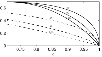
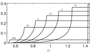
Figure 2: (a) Functions $\frac{\log\left[(c^{2})^{\alpha}+(1-c^{2})^{\alpha}\right]}{1-\alpha}$ (solid lines) and $\frac{2\log\left[\left(\frac{1+c}{2}\right)^{\alpha}+\left(\frac{1-c}{2}\right)^{\alpha}\right]}{1-\alpha}$ (dashed lines) vs $c$, for some values of $\alpha$. (b) Optimal angle $\theta_{\mathrm{opt}}$ as a function of $\alpha>0.5$ for some $c$.

We can observe that some situations discussed at the end of Sec. 2 are include in this corollary as particular cases. On the one hand, for $\alpha\to 1$, the de Vicente–Sanchez-Ruiz bound [46] is recovered. Therefore, it is optimal for qubit systems, although it was calculated treating separately $\psi$ and $\widetilde{\psi}$ without taking into account the relation between them, except through the Landau–Pollak inequality. On the other hand, for $\alpha=2$, one recovers the tight bound obtained by Bosyk et al. [47]. Therefore, we extend previous results along all the line $\beta=\alpha$ giving a semi-analytical expression for the bound.

Finally, note that using the fact that $H_{\lambda}$ decreases with $\lambda$ [10, 13, 44] one obtains the suboptimal result

Corollary 3.

In the context of Proposition 7, for any couple $(\alpha,\beta)\in\mathbb{R}_{+}^{2}$, the entropies sum is lower bounded by

$$H_{\alpha}(|\psi|^{2})+H_{\beta}(|\widetilde{\psi}|^{2})\geq\overline{{\cal B}}_{\lambda,\lambda;2}(c)\quad\mbox{with}\quad\lambda=\max(\alpha,\beta)$$ (14)

where $\overline{{\cal B}}_{\lambda,\lambda;2}(c)$ is given in Eq. (13).

This bound is clearly suboptimal, as it can be see for example in the case $(\alpha,\beta)\in\left[0\>,\>\frac{1}{2}\right]^{2}$.

In Fig. 3, we represent schematically the scope of Proposition 1, Corollaries 2 and 3 with shadowed region, solid line and dotted lines in the $\alpha$–$\beta$ plane.

Figure 3: Plane of entropic indices. The bound is tight in the square $\left[0\>,\>\frac{1}{2}\right]^{2}$ (dark grey region) and on the line $\beta=\alpha$ (solid line). Outside this region the bound is suboptimal (clear grey region) Note that previous results $(\alpha,\beta)=\left(\frac{1}{2},\frac{1}{2}\right)$,$(1,1)$ and $(2,2)$ (dots) belong to the first region, whereas the conjugacy curve (dashed line) belongs to the second one.

Note that starting from $\alpha\to\infty$ and appealing to the decreasing property of the entropy versus the index, we recover the relation

$$H_{\alpha}(|\psi|^{2})+H_{\beta}(|\widetilde{\psi}|^{2})\geq-2\log\left(\frac{1+c}{2}\right)$$ (15)

which is precisely the bound obtained by Deutsch [14] in the context of Shannon entropies, or the one given by Maassen and Uffink for any couple of indices (before being refined in the same article) [13, Eq. 9 & prop. (d)–(e)].

4 Discussion

For pure states of qubit systems, we obtain the most general entropic formulation of the uncertainty principle in terms of the sum of Rényi entropies associated with any given pair of quantum observables, namely an inequality of the form $H_{\alpha}(|\psi|^{2})+H_{\beta}(|\widetilde{\psi}|^{2})\geq{\cal B}_{\alpha,\beta;2}(c)$ where $c$ is the overlap of the transformation between the eigenspaces of the observables. Our derivation focusses on obtaining the minimum of the entropies sum and we do not use Riesz–Thorin theorem in contrast to many results in the literature. In this way, we avoid the Hölder conjugacy constraint on indices $\alpha$ and $\beta$ and our bound is tight and valid for any couple of indices. Indeed, the bound obtained is universal in the sense that it does not depend on the state of the quantum system. This is the main result of the paper, given in Propositions 7 and 9. Unfortunately, we do not always obtain an analytical expression for the bound. However, we do obtain in some domains of the plane $(\alpha,\beta)$ that the bound takes an analytical or semi-analytical expression. In effect, in Corollary 1 we present an analytical expression for the tight bound in the square $(\alpha,\beta)\in\left[0\>,\>\frac{1}{2}\right]^{2}$; whereas in Corollary 2 we show a semi-analytical expression for the tight bound on the line $\beta=\alpha$. Accordingly, we recovered many bounds derived in the literature for particular points of the plane $(\alpha,\beta)$. Moreover, using the nonincreasing property of the Rényi entropy versus the entropic index, an analytical bound is obtained, this last one being suboptimal (Corollary 3). The same propert allows also to recover the suboptimal bound primarily derived by Maassen and Uffink.

For mixed states, it is easy to extend the validity of Proposition 7 and Corollaries 1 and 2 within the domain $(\alpha,\beta)=[0,2]^{2}$ using the concavity property of Rényi entropy. Indeed for $N$-level systems, if one has a universal relation $H_{\alpha}(|\psi|^{2})+H_{\beta}(|\widetilde{\psi}|^{2})\geq\overline{{\cal B}}_{\alpha,\beta;N}$ satisfied for any pure state, with $(\alpha,\beta)\in[0\>,\>\lambda_{*}(N)]^{2}$ then one has $H_{\alpha}\left(\sum_{m}\mu_{m}|\psi^{(m)}|^{2}\right)+H_{\beta}\left(\sum_{m}\mu_{m}|\widetilde{\psi}^{(m)}|^{2}\right)\geq\sum_{m}\mu_{m}\left(H_{\alpha}(|\psi^{(m)}|^{2})+H_{\beta}(|\widetilde{\psi}^{(m)}|^{2})\right)\geq\sum_{m}\mu_{m}\overline{{\cal B}}_{\alpha,\beta;N}=\overline{{\cal B}}_{\alpha,\beta;N}$, where $\sum_{m}\mu_{m}=1$. In other words, any uncertainty formulation for pure states in the domain $(\alpha,\beta)\in[0\>,\>\lambda_{*}(N)]^{2}$ remains valid for mixed states. It remains to be studied the way of overcome this constraint in the domain of entropic indices due to the concavity property and the generalization of the results to $N$-level systems.

Acknowledgments:

SZ is grateful to the Région Rhône-Alpes (France) for the grant that enabled this work. GMB and MP acknowledge financial support from CONICET and ANPCyT (Argentina).

Appendix A Proof of Proposition 7 and Corollaries 1 and 2

A.1 Simplification of the problem

Since $\|\psi\|_{2}=1$, such a vector can be written under the form

$$\psi=\Phi({\boldsymbol{\varphi}})\,s$$ (16)

where $s\in\mathbb{S}^{(1)}$ the unit sphere on $\mathbb{R}^{2}$ (i.e. the circle) and where matrix $\Phi$ is diagonal and writes

$$\Phi(\boldsymbol{x})=\exp(\imath\,\mathrm{diag}(\boldsymbol{x}))$$ (17)

We parameterize the unitary matrix $T$ as the product of three unitary matrices (see [50, Eqs. (1)–(19)] or [49, Th. 1])

$$T=\Phi(\boldsymbol{u})\,V(\gamma_{T})\,\Phi(\boldsymbol{v})\quad\mbox{ with }V(\gamma_{T})=\left[\begin{array}[]{cc}\cos\gamma_{T}&\sin\gamma_{T}\\ &\\ -\sin\gamma_{T}&\cos\gamma_{T}\end{array}\right],\quad\gamma_{T}\in\left[0\>,\>\frac{\pi}{2}\right)$$ (18)

(the other possible angles can be taken into account playing with phases $\boldsymbol{u}$ and $\boldsymbol{v}$).

Then, from the relation (1) between $\psi$ and $\widetilde{\psi}$ and from the form (18) of $T$, one obtains

$$\widetilde{\psi}=\Phi(\boldsymbol{u})\,V(\gamma_{T})\,\Phi(\boldsymbol{v}+\boldsymbol{\varphi})\,s$$ (19)

Note first that the overlap does not depend on the phases, namely $c=\max_{k,l}|T_{lk}|=\max_{k,l}|V_{lk}(\gamma_{T})|$. The goal is then to solve the minimization problem

$${\cal B}_{\alpha,\beta;2}=\min_{\boldsymbol{\varphi},s}\left(H_{\alpha}(|\Phi(\boldsymbol{\varphi})\,s|^{2})+H_{\beta}(|\Phi(\boldsymbol{u})\,V(\gamma_{T})\,\Phi(\boldsymbol{v}+\boldsymbol{\varphi})\,s|^{2})\right)$$ (20)

The problem simplifies due to numerous invariances and symmetries.

• Invariance under a phase shift applied to the wavevector (multiplication by a matrix $\Phi$):

  $$H_{\alpha}(|\Phi(\boldsymbol{\varphi})s|^{2})+H_{\beta}(|\Phi(\boldsymbol{u})V(\gamma_{T})\Phi(\boldsymbol{v}+\boldsymbol{\varphi})|^{2})=H_{\alpha}(|s|^{2})+H_{\beta}(|V(\gamma_{T})\,\Phi(\boldsymbol{\varphi}+\boldsymbol{v})s|^{2})$$

  $\boldsymbol{\varphi}\to\boldsymbol{v}+\boldsymbol{\varphi}$ being isomorphic, minimization (20) reduces to

  $${\cal B}_{\alpha,\beta;2}=\min_{\boldsymbol{\varphi},s}\left(H_{\alpha}(|s|^{2})+H_{\beta}(|V(\gamma_{T})\,\Phi(\boldsymbol{\varphi})\,s|^{2})\right)$$ (21)

  At this step, one can notice that the bound depends only on $\gamma_{T}$.

• Additional invariance under a permutation of the components: the entropy does not depend on the order of the components, thus, playing with the phases one sees that

  $$H_{\alpha}(|s|^{2})+H_{\beta}(|V(\gamma_{T})\Phi(\boldsymbol{\varphi})s|^{2})=H_{\alpha}(|s|^{2})+H_{\beta}(|V\left(\textstyle{\frac{\pi}{2}}-\gamma_{T}\right)\Phi(\boldsymbol{\varphi}-[\pi\quad 0]^{t})s|^{2})$$

  and thus the minimization problem (21) reduces a step more,

  $${\cal B}_{\alpha,\beta;2}=\min_{\boldsymbol{\varphi},s}\left(H_{\alpha}(|s|^{2})+H_{\beta}(|V(\gamma)\,\Phi(\boldsymbol{\varphi})\,s|^{2})\right)\quad\mbox{where}\quad\gamma=\min\left(\gamma_{T}\>,\>\frac{\pi}{2}-\gamma_{T}\right)\in\left[0\>,\>\frac{\pi}{4}\right]$$ (22)

  This result prove now that the bound ${\cal B}_{\alpha,\beta;2}={\cal B}_{\alpha,\beta;2}(c)$ only depends on the overlap

  $$c=\cos\gamma=\max_{k,l=1,2}|T_{lk}|$$ (23)

• Symmetries and periodicities on $s$: Note that $s\in\mathbb{S}^{(1)}$ can write in terms of angle as $s(\theta)=[\cos\theta\quad\sin\theta]^{t}$

  • $\pi$-periodicity: clearly,

    $$H_{\alpha}(|s(\theta)|^{2})+H_{\beta}(|V(\gamma)\Phi(\boldsymbol{\varphi})s(\theta)|^{2})=H_{\alpha}(|s(\theta+\pi)|^{2})+H_{\beta}(|V(\gamma)\Phi(\boldsymbol{\varphi})s(\theta+\pi)|^{2})$$

    so that one can restrict the search to $\theta\in\left[-\frac{\pi}{2}\>,\>\frac{\pi}{2}\right]$.

  • $\frac{\pi}{2}$-symmetry: playing with the permutations and phases, it can be shown that

    $$H_{\alpha}(|s(\theta)|^{2})+H_{\beta}(|V(\gamma)\Phi(\boldsymbol{\varphi})s(\theta)|^{2})=H_{\alpha}(|s(\theta+\textstyle{\frac{\pi}{2}})|^{2})+H_{\beta}(|V(\gamma)\Phi(J\boldsymbol{\varphi})s(\theta+\textstyle{\frac{\pi}{2}})|^{2})$$

    where $J=\begin{bmatrix}0&1\\ 1&0\end{bmatrix}$, allowing one to restrict a little bit more the interval $\theta\in\left[-\frac{\pi}{4}\>,\>\frac{\pi}{4}\right]$.

  • opposite angle: we can finally note that $s(-\theta)=\Phi([0\qquad\pi]^{t})s(\theta)$ so that

    $$H_{\alpha}(|s(\theta)|^{2})+H_{\beta}(|V(\gamma)\Phi(\boldsymbol{\varphi})s(\theta)|^{2})=H_{\alpha}(|s(-\theta)|^{2})+H_{\beta}(|V(\gamma)\Phi(\boldsymbol{\varphi}+[0\quad\pi]^{t})s(-\theta)|^{2})$$

    allowing to retrict a step more to $\theta\in\left[0\>,\>\frac{\pi}{4}\right]$

  From these symmetries, the problem restricts to

  $${\cal B}_{\alpha,\beta;2}(c)\>\>=\min_{\boldsymbol{\varphi},\theta\in\left[0\>,\>\frac{\pi}{4}\right]}\left(H_{\alpha}(|s(\theta)|^{2})+H_{\beta}(|V(\gamma)\Phi(\boldsymbol{\varphi})s(\theta)|^{2}\right)\quad\mbox{where}\quad\gamma=\min\left(\gamma_{T}\>,\>\frac{\pi}{2}-\gamma_{T}\right)$$ (24)

A.2 The trivial case $c=1$

In this case, $\gamma=0$ and $V(0)=I$ the identity. Clearly for $s=[1\quad 0]^{t}$ one finds both $H_{\alpha}(|s|^{2})=0$ and $H_{\beta}(|V(0)\,\Phi(\boldsymbol{\varphi})\,s|^{2})=H_{\beta}(|s|^{2})=0$ and thus

$${\cal B}_{\alpha,\beta;2}(1)=0$$ (25)

A.3 The general nontrivial case $c<1$

In this case, one has then $0<\gamma\leq\frac{\pi}{4}$. Let us then proceed in two steps: (i) fix $s$ (i.e. $\theta$) and minimize the entropies sum over phases $\boldsymbol{\varphi}$; (ii) for the minimizing phase, that depends (in principle) on $\theta$, $\boldsymbol{\varphi}(\theta)$, determine the value of $\theta$ that minimizes the entropies sum.

A.3.1 Minimization over phase $\boldsymbol{\varphi}$

Note that phases $\boldsymbol{\varphi}$ play a role only on the term $H_{\beta}(|V(\gamma)\Phi(\boldsymbol{\varphi})s(\theta)|^{2})$. Note then that $H_{\beta}(|V(\gamma)\,\Phi(\boldsymbol{\varphi})s(\theta)|^{2})$ is invariant under multiplication of the argument by the scalar $\exp(\imath\varphi^{\prime})$, i.e. by shifting both components of $\boldsymbol{\varphi}$ by the same phase shift. Thus, without loss of generality, one can consider $\boldsymbol{\varphi}=[-\varphi_{2}\quad\varphi_{2}]^{t}$ and thus

$$\left|V(\gamma)\,\Phi(\boldsymbol{\varphi})\,s(\theta)\right|^{2}=\cos^{2}\varphi_{2}\left[\begin{array}[]{r}\cos^{2}(\gamma-\theta)\\ \sin^{2}(\gamma-\theta)\end{array}\right]+\sin^{2}\varphi_{2}\left[\begin{array}[]{r}\cos^{2}(\gamma+\theta)\\ \sin^{2}(\gamma+\theta)\end{array}\right]$$ (26)

Clearly both mappings $\varphi_{2}\mapsto-\varphi_{2}$ and $\varphi_{2}\mapsto\pi-\varphi_{2}$ leave the entropy unchanged so that, without loss of generality, one can consider $\varphi_{2}\in\left[0\>,\>\frac{\pi}{2}\right]$ only and the solutions are modulo $\pi$. The goal is then to minimize $H_{\beta}(|V(\gamma)\Phi(\boldsymbol{\varphi})s(\theta)|^{2})$ over $\varphi_{2}\in\left[0\>,\>\frac{\pi}{2}\right]$, that is equivalent to find the maximum

$$\max_{\varphi_{2}\in\left[0\>,\>\frac{\pi}{2}\right]}\frac{\left(|V(\gamma)\Phi(\boldsymbol{\varphi})s(\theta)|^{2}\right)^{\beta}}{\beta-1}$$ (27)

Note now that $\left|V(\gamma)\,\Phi(\boldsymbol{\varphi})\,s(\theta)\right|^{2}$ is a convex combination of the vectors $[\cos^{2}(\gamma-\theta)\quad\sin^{2}(\gamma-\theta)]^{t}$ and $[\cos^{2}(\gamma+\theta)\quad\sin^{2}(\gamma+\theta)]^{t}$ (see Fig. 4). Function $x\mapsto\frac{\|x\|_{\beta}^{\beta}}{\beta-1}$ being convex [44, 52], the maximum is attained on the border of the convex set defined by $\left\{\left|V(\gamma)\,\Phi(\boldsymbol{\varphi})\,s(\theta)\right|^{2}\right\}_{\varphi_{2}\in\left[0\>,\>\frac{\pi}{2}\right]}$ (see Fig. 4), namely

$$\max_{\varphi_{2}\in\left[0\>,\>\frac{\pi}{2}\right]}\frac{\left(|V(\gamma)\Phi(\boldsymbol{\varphi})s(\theta)|^{2}\right)^{\beta}}{\beta-1}=\max\left(\frac{{\cal D}_{\beta}(\gamma-\theta)}{\beta-1}\>,\>\frac{{\cal D}_{\beta}(\gamma+\theta)}{\beta-1}\right)$$ (28)

where functions ${\cal D}_{\lambda}$ are defined by

$${\cal D}_{\lambda}(\theta)=\left(\cos^{2}\theta\right)^{\lambda}+\left(\sin^{2}\theta\right)^{\lambda}$$ (29)

corresponding to $\varphi_{2}=n\frac{\pi}{2}$, $n=0,1$.

Figure 4: Vector $z=\left|V(\gamma)\,\Phi(\boldsymbol{\varphi})\,s(\theta)\right|^{2}$ lives in the segment (the convex) that link vectors $x=[\cos^{2}(\gamma-\theta)\quad\sin^{2}(\gamma-\theta)]^{t}$ and $y=[\cos^{2}(\gamma+\theta)\quad\sin^{2}(\gamma+\theta)]^{t}$. The typical behavior of a convex function $\mathbb{R}^{2}\to\mathbb{R}$ is represented by the solid line, illustrating that the maximum is attaind in the boundary of the convex set.

One can go a step further, comparing $\frac{{\cal D}_{\beta}(\gamma-\theta)}{\beta-1}$ and $\frac{{\cal D}_{\beta}(\gamma+\theta)}{\beta-1}$. To this end, consider the difference

$$\Delta(\theta,\gamma)=\frac{{\cal D}_{\beta}(\gamma-\theta)-{\cal D}_{\beta}(\gamma+\theta)}{\beta-1}$$ (30)

where $(\gamma,\theta)\in\left[0\>,\>\frac{\pi}{4}\right]^{2}$. From the obvious symmetries $\Delta(\theta,\gamma)=\Delta(\gamma,\theta)=\Delta(\frac{\pi}{4}-\theta,\frac{\pi}{4}-\gamma)$, one can restrict the study to the triangle

$$D=\{(\theta,\gamma)\in[0\>,\>\pi/4]^{2},0\leq\theta\leq\min(\gamma,\pi/4-\gamma)\}$$ (31)

as depicted in Fig. 5. Note first that $\Delta(\theta,0)=0$, then let us study the variations on the segments $\gamma=\theta_{0}-\theta$ as pictured in Fig. 5.

Figure 5: Illustration of the symmetries $\Delta(\theta,\gamma)=\Delta(\gamma;\theta)=\Delta(\pi/4-\theta,\pi/4-\gamma)=\Delta(\theta;\gamma)$. As an illustration, the point represented by a circle has three symmetric (squares) for which $\Delta$ has the same value. Thus, (the signum of) function $\Delta$ has only to be studied on domain $D$ represented by zebras and given in Eq. (31). The line in bold represents the segment $\gamma=\theta_{0}-\theta$ in $D$, where function $\Delta$ is studied.

A simple derivation leads to

$$\frac{\partial\Delta(\theta,\theta_{0}-\theta)}{\partial\theta}=\frac{2\beta\sin(4\theta-2\theta_{0})\left(\left(\sin^{2}(2\theta-\theta_{0})\right)^{\beta}-\left(\cos^{2}(2\theta-\theta_{0})\right)^{\beta}\right)}{\beta-1}$$ (32)

Since $0\leq\theta_{0}/2\leq\theta\leq\theta_{0}\leq\pi/4$, on has $0\leq 2\theta-\theta_{0}\leq\pi/4$, and thus on the one hand $\sin(4\theta-2\theta_{0})\geq 0$ while on the other hand $\sin(2\theta-\theta_{0})\leq\cos(2\theta-\theta_{0})$. This proves that the derivative is positive, and thus that $\Delta(\theta,\theta_{0}-\theta)$ increases with $\theta$. Together with $\Delta(\theta_{0},0)=0$ and the symmetries, we have proved then that in the whole square $\left[0\>,\>\frac{\pi}{4}\right]^{2}$ one has $\Delta(\theta,\gamma)\geq 0$, i.e.  $\frac{{\cal D}(\gamma-\theta)}{\beta-1}\geq\frac{{\cal D}(\gamma+\theta)}{\beta-1}$. This finishes to prove that

$$\min_{\varphi_{2}\in\left[0\>,\>\frac{\pi}{2}\right]}H_{\beta}(|V(\gamma)\Phi(\boldsymbol{\varphi})s(\theta)|^{2})=\frac{\log{\cal D}_{\beta}(\gamma-\theta)}{1-\beta}$$ (33)

obtained for

$$\varphi_{2,\mathrm{opt}}=0$$ (34)

Note that due to the invariance of the entropies sum under the multiplication of the wavevector by a scalar $\exp(\imath\varphi^{\prime})$, in some sense there exists a “unique” phase $\boldsymbol{\varphi}$ minimizing the entropies sum when $s$ is fixed. Moreover, “this” phase does not depend on $s$.

A.3.2 Minimization over the angle $\theta$

Before specializing the problem in different parts of the plane $(\alpha,\beta)$, one can simplify one step more the interval in $\theta$ where the minimum of the entropies sum has to be sought. From the preceding section, minimization (24) reduces to

$${\cal B}_{\alpha,\beta;2}(c)=\min_{\theta\in\left[0\>,\>\frac{\pi}{4}\right]}\left(\frac{\log{\cal D}_{\alpha}(\theta)}{1-\alpha}+\frac{\log{\cal D}_{\beta}(\gamma-\theta)}{1-\beta}\right)\quad\mbox{with}\quad D_{\lambda}(\theta)=\left(\cos^{2}\theta\right)^{\lambda}+\left(\sin^{2}\theta\right)^{\lambda}$$ (35)

Deriving the functional to minimize gives

$$\frac{\partial}{\partial\theta}\left(\frac{\log{\cal D}_{\alpha}(\theta)}{1-\alpha}+\frac{\log{\cal D}_{\beta}(\gamma-\theta)}{1-\beta}\right)=\frac{{\cal D}_{\alpha}^{\prime}(\theta)}{(1-\alpha)\,{\cal D}_{\alpha}(\theta)}-\frac{{\cal D}_{\beta}^{\prime}(\gamma-\theta)}{(1-\beta)\,{\cal D}_{\beta}(\gamma-\theta)}$$ (36)

where the derivative in $\theta$ of functions ${\cal D}_{\lambda}$ writes

$${\cal D}_{\lambda}^{\prime}(\theta)\>\equiv\>\frac{\partial{\cal D}_{\lambda}}{\partial\theta}=\lambda\sin(2\theta)\,\left(\left(\sin^{2}\theta\right)^{\lambda-1}-\left(\cos^{2}\theta\right)^{\lambda-1}\right)$$ (37)

Since $\theta\in[0\>,\>\pi/4]$, one has both $\sin(2\theta)\geq 0$ and $\sin^{2}\theta\leq\cos^{2}\theta$ and thus the first fraction of the right-hand side (rhs) of (36) is positive. Moreover, $\theta-\gamma\in[-\pi/4\>,\>\pi/4]$ and thus by the same reasoning the second fraction of the rhs of (36) has the same signum as $\sin(2(\gamma-\theta))$. Thus, for $\theta\in(\gamma\>,\>\pi/4]$ the entropies sum is increasing. Necessarily the minimum of the entropies sum is given by $0\leq\theta\leq\gamma$, reducing the interval where $\theta$ has to be sought, i.e.

$${\cal B}_{\alpha,\beta;2}(c)=\min_{\theta\in\left[0\>,\>\gamma\right]}\left(\frac{\log{\cal D}_{\alpha}(\theta)}{1-\alpha}+\frac{\log{\cal D}_{\beta}(\gamma-\theta)}{1-\beta}\right)$$ (38)

At this step, the minimum of (38) can only be sought numerically, leading to Proposition 7.

One can go a step further in special cases as we will see now.

A.4 Special context $(\alpha,\beta)\in\left[0\>,\>\frac{1}{2}\right]^{2}$.

Let us start from Eq. (36), that gives the second derivative of the function to be minimize under the form

$$\frac{\partial^{2}}{\partial\theta^{2}}\left(\frac{\log{\cal D}_{\alpha}(\theta)}{1-\alpha}+\frac{\log{\cal D}_{\beta}(\gamma-\theta)}{1-\beta}\right)=\frac{{\cal K}_{\alpha}(\theta)}{\left({\cal D}_{\alpha}(\theta)\right)^{2}}+\frac{{\cal K}_{\beta}(\gamma-\theta)}{\left({\cal D}_{\beta}(\gamma-\theta)\right)^{2}}$$ (39)

where functions ${\cal K}_{\lambda}=\left({\cal D}_{\lambda}^{\prime\prime}\,{\cal D}_{\lambda}-{\cal D}_{\lambda}^{\prime\,2}\right)/(1-\lambda)$ writes

$${\cal K}_{\lambda}(\theta)=\frac{2\,\lambda}{1-\lambda}\left((2\lambda-1)\left(\frac{\sin^{2}(2\theta)}{4}\right)^{\lambda-1}-\left(\cos^{2}\theta\right)^{2\lambda-1}\!-\left(\sin^{2}\theta\right)^{2\lambda-1}\right)$$ (40)

(one uses alternatively the fact that $\cos^{2}\theta-\sin^{2}\theta=2\cos^{2}\theta-1=1-2\sin^{2}\theta$ and the identities $\cos^{2}\theta\sin^{2}\theta=\cos^{2}\theta-\cos^{4}\theta=\sin^{2}\theta-\sin^{4}\theta$).

For $\lambda\leq\frac{1}{2}$, since one has then also $\lambda<1$ we can immediately conclude that the second derivative in $\theta$ of the entropies sum is strictly negative, so that function $\theta\mapsto\left(\frac{\log{\cal D}_{\alpha}(\theta)}{1-\alpha}+\frac{\log{\cal D}_{\beta}(\gamma-\theta)}{1-\beta}\right)$ is concave on $\theta\in[0\>,\gamma]$ (the opposite function is convex) [52]. Thus, the minimum (the maximum of the oposite) is attain in the border of the convex line $[0\>,\gamma]$, i.e. either for $\theta=0$, or for $\theta=\gamma$. It remains then to compare the values of the function at these extremal points, i.e.  from (38)–(29) to compare $\frac{\log{\cal D}_{\alpha}(\gamma)}{1-\alpha}$ and $\frac{\log{\cal D}_{\beta}(\gamma)}{1-\beta}$ with $D_{\lambda}$ given in Eq. (7). Since the Rényi entropy $H_{\lambda}$ is a decreasing function versus $\lambda$ [10, 13, 44], together with the expression (29) of $D_{\lambda}$ and $c=\cos\gamma$ one obtains Corollary 1.

A.5 Semi-analytical results when $\alpha=\beta$.

In order to simplify the notation, let us denote the function to minimize as

$${\cal F}_{\alpha}(\theta)=\frac{\log{\cal D}_{\alpha}(\theta)+\log{\cal D}_{\alpha}(\gamma-\theta)}{1-\alpha}$$ (41)

with ${\cal D}_{\alpha}$ defined in Eq. (29), so that the problem is to minimize ${\cal F}_{\alpha}$ over $\theta\in[0\>,\>\gamma]$. One can go a step further observing the trivial symmetry ${\cal F}_{\alpha}(\theta)={\cal F}_{\alpha}(\gamma-\theta)$, so the the problem reduces to

$${\cal B}_{\alpha,\alpha;2}(c)=\min_{\theta\in\left[0\>,\>\frac{\gamma}{2}\right]}{\cal F}_{\alpha}(\theta)$$ (42)

Since the case $(\alpha,\beta)\in[0\>,\>\frac{1}{2}]^{2}$ is already treated, one concentrates here in the context $\alpha=\beta>\frac{1}{2}$. Recall also that we exclude here the case $\alpha=1$: it will be recover by taking the limit $\alpha\to 1$.

Deriving ${\cal F}_{\alpha}$ versus $\theta$ leads to

$${\cal F}_{\alpha}^{\prime}(\theta)=\frac{\partial}{\partial\theta}{\cal F}_{\alpha}(\theta)=\frac{1}{1-\alpha}\left(\frac{{\cal D}_{\alpha}^{\prime}(\theta)}{{\cal D}_{\alpha}(\theta)}-\frac{{\cal D}_{\alpha}^{\prime}(\gamma-\theta)}{{\cal D}_{\alpha}(\gamma-\theta)}\right)$$ (43)

where ${\cal D}^{\prime}_{\alpha}$ was already explicited in Eq. (37). ${\cal F}_{\alpha}^{\prime}$ clearly vanish when $\theta=\frac{\gamma}{2}$ which gives a possible solution. The question now is to determine if the extremum is a global minimum or not.

A.5.1 When $c=1/\sqrt{2}$

In this case, $\gamma=\frac{\pi}{4}$ and it is easy to see that ${\cal D}_{\alpha}^{\prime}(0)={\cal D}_{\alpha}^{\prime}(\gamma)=0$. Thus, $\theta=0$ gives another solution to ${\cal F}_{\alpha}^{\prime}(\theta)=0$.

We observe then the following behaviours, already noticed in [31] :

• $\theta=0$ is the unique solution for $\alpha<\alpha^{\dagger}\approx 1.430$, leading to the bound $\frac{\log\left[c^{2\alpha}+(1-c^{2})^{\alpha}\right]}{1-\alpha}=\log 2$.

• When $\alpha>\alpha^{\dagger}$ the unique solution is given by $\theta=\frac{\gamma}{2}$, leading to the bound $\frac{2\,\log\left[\left(\frac{1+c}{2}\right)^{\alpha}+\left(\frac{1-c}{2}\right)^{\alpha}\right]}{1-\alpha}=\frac{2\,\log\left[\left(\frac{2+\sqrt{2}}{4}\right)^{\alpha}+\left(\frac{2-\sqrt{2}}{4}\right)^{\alpha}\right]}{1-\alpha}$.

• When $\alpha=\alpha^{\dagger}$, there is a phase transition: both $\theta=0$ and $\theta=\frac{\gamma}{2}$ give the minimum bound $\log 2$, while $\alpha^{\dagger}$ is the unique solution of $\frac{2\,\log\left[\left(\frac{2+\sqrt{2}}{4}\right)^{\alpha}+\left(\frac{2-\sqrt{2}}{4}\right)^{\alpha}\right]}{1-\alpha}=\log 2$. Note that the unicity is insured from the the fact that the entropy is a decreasing function of the index [10, 13, 44].

A.5.2 When $c\in(1/\sqrt{2}\>,\>1)$

In this case, one still has ${\cal D}_{\alpha}^{\prime}(0)=0$ but clearly for any $\theta\in\left(0\>,\>\frac{\pi}{4}\right)$, $\frac{{\cal D}_{\alpha}^{\prime}(\theta)}{1-\alpha}>0$. In other words, ${\cal F}_{\alpha}^{\prime}(0)<0$ so that $\theta=0$ cannot be a solution to ${\cal F}_{\alpha}^{\prime}(\theta)=0$: all the possible solutions are then in $\left(0\>,\>\frac{\gamma}{2}\right]$.

We observe numerically the following behavior: For any fixed $c$, there exist a $\alpha^{\star}(c)$ so that

• for $\alpha\in(0.5\>,\>\alpha^{\star}(c))$, the optimal angle $\theta_{\mathrm{opt}}(\alpha)$ is in $\left(0\>,\>\frac{\gamma}{2}\right)$ and can only be numerically seek. The bound is then numerically expressed as well. Moreover, $\theta_{\mathrm{opt}}(\alpha)$ increases continuously from $0$ to $\frac{\gamma}{2}$.

• For $\alpha\geq\alpha^{\star}(c)$ the only minimum is given for $\theta=\frac{\gamma}{2}$, leading to the bound $\frac{2\,\log\left[\left(\frac{1+c}{2}\right)^{\alpha}+\left(\frac{1-c}{2}\right)^{\alpha}\right]}{1-\alpha}$; thus, there is no transition phase in this context.

Appendix B Expression of the minimizers

B.1 Proof of Proposition 9

Let us first recall that the entropies sum is insensitive to the multiplication of the wavector by a scalar $e^{\imath\varphi}$, and thus from a minimizer $\psi_{0}$ we will obtain families of minimizers of the form $\{e^{\imath\varphi}\psi_{0}\}_{\varphi\in[0\>,\>2\pi)}$.

Recall that any unitary matrix $T$ can be parameterized under the form

$$T=\Phi(\boldsymbol{u})\,V(\gamma_{T})\,\Phi(\boldsymbol{v})\quad\mbox{with}\quad V(\gamma_{T})=\left[\begin{array}[]{cc}\cos\gamma_{T}&\sin\gamma_{T}\vspace{2mm}\\ -\sin\gamma_{T}&\cos\gamma_{T}\end{array}\right],\quad\Phi(\boldsymbol{x})=\exp(\imath\,\mathrm{diag}(\boldsymbol{x})),\quad\gamma_{T}\in\left[0\>,\>\frac{\pi}{2}\right]$$ (44)

(see [50, Eqs. (1)–(19)] or [49, Th. 1]). Let us denote by $\{\theta_{\mathrm{opt}}^{(i)}\}_{i\in{\cal I}}$, the ensemble of the minimizers angles in $[0\>,\>\gamma]$ of Eq. (6)–Eq. (38) where ${\cal I}$ indices each solution.

• Case $\gamma_{T}=\gamma\in\left[0\>,\>\frac{\pi}{4}\right]$. We have that $T\psi=\Phi(\boldsymbol{u})V(\gamma)\Phi(\boldsymbol{v})\psi$ so that an ensemble of minimizers takes the form $\left\{e^{\imath\varphi}\Phi(-\boldsymbol{v})s(\theta_{\mathrm{opt}}^{(i)})\right\}_{i\in{\cal I},\varphi\in\left[0\>,\>2\pi\right)}$.

  • Symmetry $\theta\to-\theta$: From the study of the preceding section, it is immediate that
    $\left\{e^{\imath\varphi}\Phi(-\boldsymbol{v}+[0\quad\pi]^{t})s(-\theta_{\mathrm{opt}}^{(i)})\right\}_{i\in{\cal I},\varphi\in\left[0\>,\>2\pi\right)}$ is also a family of minimizers. It turns out that it is the same family, than that obtained from the $\theta_{\mathrm{opt}}^{(i)}$.

  • Symmetry $\theta\to\theta+\frac{\pi}{2}$: From the preceding section, from angles $\theta_{\mathrm{opt}}^{(i)}$ one obtains now the family of minimizers $\left\{e^{\imath\varphi}\Phi(-\boldsymbol{v})s\left(\theta_{\mathrm{opt}}^{(i)}+\frac{\pi}{2}\right)\right\}_{i\in{\cal I},\varphi\in\left[0\>,\>2\pi\right)}$.

  • Symmetry $\theta\to\theta+\pi$: Clearly, one obtains the same families (starting respectively from the $\theta_{\mathrm{opt}}^{(i)}$ and from the the $\theta_{\mathrm{opt}}^{(i)}+\frac{\pi}{2}$).

  In a conclusion, for $\gamma_{T}=\gamma$ the minimizers take the form

  $$\psi_{\mathrm{opt}}^{(i,\varphi,n)}=e^{\imath\varphi}\Phi(-\boldsymbol{v})\begin{bmatrix}\cos\left(\theta_{\mathrm{opt}}^{(i)}+n\textstyle{\frac{\pi}{2}}\right)\vspace{2.5mm}\\ \sin\left(\theta_{\mathrm{opt}}^{(i)}+n\textstyle{\frac{\pi}{2}}\right)\end{bmatrix}\quad\mbox{with}\quad i\in{\cal I},\quad n=0,1\quad\mbox{and}\quad\varphi\in[0\>,\>2\pi)$$

• Case $\gamma_{T}=\frac{\pi}{2}-\gamma\in\left[0\>,\>\frac{\pi}{4}\right]$. We have now $T\psi=\Phi(\boldsymbol{u})JV(\gamma)\Phi(\boldsymbol{v}+[0\quad\pi]^{t})\psi$ so that an ensemble of minimizers takes the form $\left\{e^{\imath\varphi}\Phi(-\boldsymbol{v}-[0\quad\pi]^{t})s(\theta_{\mathrm{opt}}^{(i)})\right\}_{i\in{\cal I},\varphi\in\left[0\>,\>2\pi\right)}=\left\{e^{\imath\varphi}\Phi(-\boldsymbol{v})s(-\theta_{\mathrm{opt}}^{(i)})\right\}_{i\in{\cal I},\varphi\in\left[0\>,\>2\pi\right)}$. Then, following the same steps than before, one obtains in this case the family of minimizers

  $$\psi_{\mathrm{opt}}^{(i,\varphi,n)}=e^{\imath\varphi}\Phi(-\boldsymbol{v})\begin{bmatrix}\cos\left(-\theta_{\mathrm{opt}}^{(i)}+n\textstyle{\frac{\pi}{2}}\right)\vspace{2.5mm}\\ \sin\left(-\theta_{\mathrm{opt}}^{(i)}+n\textstyle{\frac{\pi}{2}}\right)\end{bmatrix}\quad\mbox{with}\quad i\in{\cal I},\quad n=0,1\quad\mbox{and}\quad\varphi\in[0\>,\>2\pi)$$

One can unify both cases by noting than the signum before the angle $\theta_{\mathrm{opt}}^{(i)}$ is nothing moe than $\mathrm{sign}\left(\frac{\pi}{4}-\gamma_{T}\right)$, leading to the expression given in Proposition 9.

B.2 A step more in the case $\alpha=\beta$.

One has seen numerically the existence of a unique optimal angle $\theta_{\mathrm{opt}}\in\left[0\>,\>\frac{\gamma}{2}\right]$ (with $\gamma=\arccos c$) leading to the minimal bound of the entropies sum. Moreover, we have seen that the entropies sum is invariant under the transformation $\theta\to\gamma-\theta$. This leads to the possible angles represented in Fig. 6(b), respectively for $\gamma_{T}\in\left[0\>,\>\frac{\pi}{4}\right]$ (circles) and $\gamma_{T}\in\left[\frac{\pi}{4}\>,\>\frac{\pi}{2}\right]$ (crosses). As a conclusion,

$$\theta_{\mathrm{opt}}^{(i)}=\frac{\gamma}{2}+i\left(\frac{\gamma}{2}-\theta_{\mathrm{opt}}\right)\quad\mbox{with}\quad i\in{\cal I}=\{-1,1\},$$

leading to the minimizers given in corolary 2.

Figure 6: (a) Angles issued from the optimal one in the case where $\gamma_{T}\in\left[0\>,\>\frac{\pi}{4}\right]$ (circle) and where $\gamma_{T}\in\left[\frac{\pi}{4}\>,\>\frac{\pi}{2}\right]$ (crosses) in the general case. For sake of readness, in this illustration we assume that $\theta_{\mathrm{opt}}$ is unique. (b) Same as in (a), when $\alpha=\beta$, taking into account the symmetries in this special case.

References

- [1] W. Heisenberg. Über den anschaulichen inhalt der quantentheoretischen kinematik und mechanik. Zeitschrift für Physik A, 43(3-4):172–198, March 1927.
- [2] E. H. Kennard. Zur quantenmechanik einfacher bewegungstypen. Zeitschrift für Physik, 44(4-5):326–352, April 1927.
- [3] H. P. Robertson. The uncertainty principle. Physical Review Letters, 34(1):163–164, July 1929.
- [4] G. Samorodnitsky and M. S. Taqqu. Stable Non-Gaussian Random Processes. Stochastic Models with infinite Variance. Chapman & Hall, New-York, 1994.
- [5] A. Luis. Complementary and certainty relations for two-dimensional systems. Physical Review A, 64(1):012103, July 2001.
- [6] A. Luis. Effect of fluctuations measures on the uncertainty relations between two observables: Different measures lead to opposite conclusions. Physical Review A, 84(3):034101, September 2011.
- [7] S. Zozor. Bruit, Non-linéaire et Information : quelques résultats. Habilitation à Diriger des Recherches, Institut National Polytechnique de Grenoble, Grenoble, France, June 2012.
- [8] C. E. Shannon. A mathematical theory of communication. The Bell System Technical Journal, 27:623–656, October 1948.
- [9] A. Rényi. On measures of entropy and information. in Proceeding of the 4th Berkeley Symposium on Mathematical Statistics and Probability, 1:547–561, 1961.
- [10] T. M. Cover and J. A. Thomas. Elements of Information Theory. John Wiley & Sons, Hoboken, New Jersey, 2nd edition, 2006.
- [11] I. I. Hirschman. A note on entropy. American Journal of Mathematics, 79(1):152–156, January 1957.
- [12] I. Bialynicki-Birula and J. Mycielski. Uncertainty relations for information entropy in wave mechanics. Communications in Mathematical Physics, 44(2):129–132, June 1975.
- [13] H. Maassen and J. B. M. Uffink. Generalized entropic uncertainty relations. Physical Review Letters, 60(12):1103–1106, March 1988.
- [14] D. Deutsch. Uncertainty in quantum measurements. Physical Review Letters, 50(9):631–633, February 1983.
- [15] I. Bialynicki-Birula. Entropic uncertainty relations. Physics Letters, 103A(5):253–254, July 1984.
- [16] A. K. Rajagopal. The Sobolev inequality and the Tsallis entropic uncertainty relation. Physics Letters A, 205(1):32–36, September 1995.
- [17] M. Portesi and A. Plastino. Generalized entropy as measure of quantum uncertainty. Physica A, 225(3-4):412–430, April 1996.
- [18] I. Bialynicki-Birula. Formulation of the uncertainty relations in terms of the Rényi entropies. Physical Review A, 74(5), November 2006.
- [19] S. Zozor and C. Vignat. On classes of non-Gaussian asymptotic minimizers in entropic uncertainty principles. Physica A, 375(2):499–517, March 2007.
- [20] S. Zozor, M. Portesi, and C. Vignat. Some extensions to the uncertainty principle. Physica A, 387(18-19):4800–4808, August 2008.
- [21] S. Wehner and A. Winter. Entropic uncertainty relations – a survey. New Journal of Physics, 12:025009, February 2010.
- [22] K. D. Sen, editor. Statistical Complexity. Application in Electronic Structure. Springer Verlag, New-York, 2011.
- [23] J. S. Dehesa, S. López-Rosa, and D. Manzano. Entropy and complexity analyses of -dimensional quantum systems. In K. D. Sen, editor, Statistical Complexities: Application to Electronic Structure. Springer, Berlin, 2010.
- [24] E. Romera, J. C. Angulo, and J. S. Dehesa. Fisher entropy and uncertaintylike relationships in many-body systems. Physical Review A, 59(5):4064–4067, May 1999.
- [25] E. Romera, P. Sánchez-Moreno, and J. S. Dehesa. Uncertainty relation for Fisher information of -dimensional single-particle systems with central potentials. Journal of Mathematical Physics, 47(10):103504, October 2006.
- [26] P. Sánchez-Moreno, R. González-Férez, and J. S. Dehesa. Improvement of the Heisenberg and Fisher-information-based uncertainty relations for -dimensional potentials. New Journal of Physics, 8:330, December 2006.
- [27] S. Zozor, M. Portesi, P. Sánchez-Moreno, and J. S. Dehesa. Position-momentum uncertainty relation based on moments of arbitrary order. Physical Review A, 83(5):052107, May 2011.
- [28] B. Ricaud and B. Torrésani. Refined support and entropic uncertainty inequalities. arXiv:1210.7711 [cs.IT], 2012.
- [29] A. E. Rastegin. Notes on entropic uncertainty relations beyond the scope of Riesz’ therorem. International Journal of Theoretical Physics, 51(4):1300–1314, April 2012.
- [30] G. M. Bosyk, M. Portesi, and A. Plastino. Collision entropy and optimal uncertainty. Physical Review A, 65(1):012108, January 2012.
- [31] G. M. Bosyk, M. Portesi, F. Holik, and A. Plastino. On the connection between complementary and uncertainty principle in the Mach-Zehnder interferometric setting. Physica Scripta, 87(6):065002, june 2013.
- [32] M. Elad and A. M. Bruckstein. A generalized uncertainty principle and sparse representation in pairs of bases. IEEE Transactions on Information Theory, 48(9):2558–2567, September 2002.
- [33] S. Ghobber and P. Jaming. On uncertainty principles in the finite dimensional setting. Linear Algebra and its Applications, 435(15):751–768, August 2011.
- [34] I. Bengtsson and K. Życzkowski. Geometry of Quantum States: An Introduction to Quantum Entanglement. Cambridge University Press, Cambridge, 2006.
- [35] J.-F. Bercher. Source coding with escort distributions and Rényi entropy bounds. Physics Letters A, 373(36):3235–3238, August 2009.
- [36] R. G. Baraniuk, P. Flandrin, A. J. E. M. Jansen, and O. J. J. Michel. Measuring time-frequency information content using the Rényi entropies. IEEE Transactions on Information Theory, 47(4):1391–1409, May 2001.
- [37] A. O. Hero III, B. Ma, O. J. J. Michel, and J. Gorman. Application of entropic spanning graphs. IEEE Signal Processing Magazine, 19(5):85–95, September 2002.
- [38] D. Harte. Multifractals: Theory and applications. Chapman & Hall / CRC, Boca Raton, 1st edition, 2001.
- [39] H. G. E. Hentschel and I. Procaccia. The infinite number of generalized dimensions of fractals and strange attractor. Physica D, 8(3):435–444, September 1983.
- [40] P. Jizba and T. Arimitsu. The world according to Rényi: thermodynamics of multifractal systems. Annals of Physics, 312(1):17–59, July 2004.
- [41] A. G. Bashkirov. Maximum Rényi entropy principle for systems with power-law hamiltonians. Physical Review Letters, 93(13), September 2004.
- [42] P. Jizba. Information theory and generalized statistics. In H.-T. Elze, editor, Decoherence and Entropy in Complex Systems: Selected Lectures from DICE (Decoherence, Information, Complexity and Entropy; Piombino, Italy, September 2-6, 2002), volume 633 of Lecture Notes in Physics, pages 362–376, Heidelberg, 2003. Springer Verlag.
- [43] A. S. Parvan and T. S. Biró. Extensive Rényi statistics from non-extensive entropy. Physics Letters A, 340(5-6):375–387, June 2005.
- [44] G. Hardy, J. E. Littlewood, and G. Pólya. Inequalities. Cambridge University Press, Cambridge, UK, 2nd edition, 1952.
- [45] A. Luis. Quantum properties of exponential states. Physical Review A, 75(5), May 2007.
- [46] J. I. de Vicente and J. Sánchez-Ruiz. Improved bounds on entropic uncertainty relations. Physical Review E, 77(4):04110, April 2008.
- [47] G. M. Bosyk, M. Portesi, A. Plastino, and S. Zozor. Comment on “improved bounds on entropic uncertainty relations”. Physical Review A, 84(5):056101, November 2011.
- [48] G. C. Ghirardi, L. Marinatto, and R. Romano. An optimal entropic uncertainty relation in a two-dimensional Hilbert space. Physics Letters A, 317(1-2):32–36, october 2003.
- [49] P. Diţă. Factorization of unitary matrices. Journal of Physics A, 36(11):2781–2789, march 2003.
- [50] C. Jarlskog. A recursive parametrization of unitary matrices. Journal of Mathematical Physics, 46(10):103508, october 2005.
- [51] H. J. Landau and H. O. Pollak. Prolate spheroidal wave functions, Fourier analysis and uncertainty – ii. The Bell System Technical Journal, 40(1):65–84, January 1961.
- [52] P. S. Bullen. Handbook of Means and Their Inequalities. Kluwer, Dordrecht, 2003.