Lennard-Jones systems near solid walls: Computing interfacial free energies from molecular simulation methods

Abstract

Different computational techniques in combination with molecular dynamics computer simulation are used to to determine the wall-liquid and the wall-crystal interfacial free energies of a modified Lennard-Jones (LJ) system in contact with a solid wall. Two different kinds of solid walls are considered: a flat structureless wall and a structured wall consisting of an ideal crystal with the particles rigidly attached to fcc lattice sites. Interfacial free energies are determined by a thermodynamic integration scheme, the anisotropy of the pressure tensor, the non-equilibrium work method based on Bennett acceptance criteria, and a method using Cahn’s adsorption equations based on the interfacial thermodynamics of Gibbs. For the flat wall, interfacial free energies as a function of different densities of the LJ liquid and as a function of temperature along the coexistence curve are calculated. In case of a structured wall, the interaction strength between the wall and the LJ system and the lattice constant of the structured wall are varied. Using the values of the wall-liquid and wall-crystal interfacial energies along with the value for the crystal-liquid interfacial free energy determined previously for the same system by the “cleaving potential method”, we obtain the contact angle as a function of various parameters; in particular the conditions are found under which partial wetting occurs.

I Introduction

Interfacial free energies between a crystal or liquid in contact with a solid wall are a key determinant of several interfacial phenomena such as wetting degennes85 , adhesion and heterogeneous nucleation zettlemoyer69 ; abraham74 ; kashchiev00 . However, they are difficult to determine in experiments and very few results are available in the literature (see e.g. adamson97 ; navascues79 ; howe97 ). Therefore, molecular simulation techniques such as Molecular Dynamics (MD) and Monte Carlo (MC) frenkel-smit02 ; landau-binder00 ; allen-tildesley87 play an important role to elucidate interfacial phenomena. Since molecular simulations can be used to determine the same thermodynamic quantity via various computational strategies, reliable estimates of the desired quantities are obtained by comparing the results obtained from the different methods. In this work, our objective is to employ several different computational techniques for obtaining reliable estimates of the wall-liquid and wall-crystal interfacial free energies, in the following denoted by $\gamma_{\text{wl}}$ and $\gamma_{\text{wc}}$, respectively.

In order to calculate $\gamma_{\text{wl}}$, mechanical techniques can be employed to compute the interfacial tension from the pressure anisotropy (PA) kirkwood49 . Several authors have used this technique to calculate $\gamma_{\rm wl}$ for both hard-sphere henderson84 ; courtemanche93 ; miguel06 and Lennard-Jones (LJ) systems sikkenk88 ; bakker89 ; nijmeijer90 ; bruin91 ; crevecoeur95 ; tang95 ; varnik00 . Since, in general, the interfacial tension is not equal to the interfacial free energy shuttleworth50 , except in case of a liquid in contact with a static wall, the mechanical approach fails in situations involving liquid in contact with a wall consisting of a “fully interacting solid phase” laird10 or for a crystal in contact with a solid wall tiller91 . Another drawback is the massive computational effort needed to obtain reliable results, since the interfacial tension being the difference of the normal and tangential pressure profiles is very sensitive to small numerical errors deb10 ; deb11 .

In contrast to the PA method, thermodynamic integration (TI) techniques frenkel-smit02 ; benjamin-horbach2012 are applicable to a wider class of systems including systems where the liquid interacts with an elastic wall or for wall-crystal interfaces. Various TI schemes have been proposed for the calculation of $\gamma_{\rm wl}$ and $\gamma_{\rm wc}$ and applied to systems modelled by hard-sphere, LJ or other soft interaction potentials benjamin-horbach2012 ; heni99 ; fort-djik06 ; laird07 ; leroy09 . While the TI method is simple to understand and easy to implement in MD or MC simulations, care has to be taken that the switching protocol that transforms the initial to the final state is reversible and does not lead to any hysteresis. As a result, the computational load can be considerable.

A less computationally expensive method, which does not require the constraint of a reversible switching protocol, is the non-equilibrium work method. In 1997, Jarzynski showed that one can extract the equilibrium free energy difference between two states from an exponential average of the non-equilibrium work performed on the system during a transformation from one state to another jarzynski1997 . However, to obtain an accurate estimate of the free energy difference using the Jarzynski equality (JE), the tail of the work probability distribution must be well sampled, which is possible only if an extremely large number of independent runs are performed jarzynski06 . Therefore, in general, a direct application of the Jarzynski equality leads to a significant bias and variance in the free energy estimates fox03 . Shirts et al. shirts-pande2005 demonstrated that one can overcome this disadvantage by carrying out both forward and backward transformations between the two states and then estimating the equilibrium free energy difference using the Bennett acceptance ratio (BAR) bennett1976 . The BAR method has been applied to obtain the crystal-liquid interfacial free energy for both hard sphere and LJ systems davidchack2010 ; musong2006 . However, to the best of our knowledge there have been no studies where non-equilibrium work approaches have been used to compute $\gamma_{\text{wl}}$ or $\gamma_{\text{wc}}$.

If interfacial free energies are needed at many points along a coexistence curve, say, the TI and BAR methods would both be computationally expensive. Recently, Laird and others have obtained $\gamma_{\text{wl}}$ for a hard-sphere system by integrating along a pressure curve laird10 and the crystal-liquid interfacial free energy for LJ systems as a function of temperature along the coexistence curve laird09 using the “Gibbs-Cahn integration” method. This technique is based on adsorption equations derived by Cahn cahn79 to extend Gibbs’s interfacial thermodynamics gibbs57 . The “Gibbs-Cahn integration” (GC) method requires that the values for the interfacial free energy is already known at one point along the curve, then at the remaining points the free energies can be determined by integrating along the curve. While, Laird and Davidchack computed $\gamma_{\text{wl}}$ for hard spheres in contact with a hard wall, there have been no corresponding studies for LJ systems.

Although, the above described methods can be employed to determine $\gamma_{\text{wl}}$ and $\gamma_{\text{wc}}$, a priori it is not known which technique yields the most accurate results. To investigate this issue, we use different computational methods to arrive at reliable estimates for $\gamma_{\text{wl}}$ and $\gamma_{\text{wc}}$ and also discuss the computational efficiency of each method. To this end, we compute $\gamma_{\text{wc}}$ and $\gamma_{\text{wl}}$ for a LJ system in contact with solid walls from non-equilibrium work measurements using the JE and BAR methods and compare the results with a TI scheme devised in our earlier work benjamin-horbach2012 . The interfacial free energies are computed for both a bulk LJ liquid and a bulk LJ face centred cubic crystal oriented along the (111) direction. We consider two kinds of solid walls: one is a flat structureless wall and the other one is a structured wall consisting of particles rigidly attached to fcc lattice sites with the (111) orientation of the wall in contact with the system. In this work, $\gamma_{\text{wl}}$ and $\gamma_{\text{wc}}$ are obtained by our TI scheme and non-equilibrium work methods; the wall-liquid interfacial free energy, $\gamma_{\text{wl}}$ is also determined via the GC method as well as the PA technique. Results from the four different approaches are compared with each other.

If in addition to the wall-liquid and wall-crystal interfacial free energies, one has knowledge about the crystal-liquid interfacial free energy, $\gamma_{\text{cl}}$, a direct determination of the degree of wetting of a solid surface by a substance can be obtained from Young’s equation young1805 ,

$$\gamma_{\text{wc}}+\gamma_{\text{cl}}\cos\theta_{\text{c}}=\gamma_{\text{wl}}\,$$ (1)

with $\theta_{\rm c}$ the contact angle. The contact angle controls whether crystal nucleation from the bulk liquid occurs preferably via homogeneous nucleation corresponding to complete drying ($\theta_{\rm c}=180^{\circ}$) or at the wall via heterogeneous nucleation corresponding to partial wetting ($0^{\circ}<\theta_{\rm c}<90^{\circ}$) or partial drying ($90^{\circ}<\theta<180^{\circ}$) scenarios. However, to obtain $\theta_{\rm c}$ from Eq. (1), the value for $\gamma_{\text{cl}}$ is also needed. Therefore, we carried out simulations using a form of the LJ potential first introduced by Broughton and Gilmer broughton-gilmer86 ; davidchack-laird03 ; laird09 ; asano-fuchizaki09 ; asano-fuchizaki12 , for which $\gamma_{\text{cl}}$ has already been determined using the “cleaving potential” approach davidchack-laird03 as well as the Gibbs Cahn integration technique laird09 .

In the following, we introduce the details of the model potentials considered in this work (Sec. II), then describe the non-equilibrium work method and the Gibb’s Cahn integration technique (Sec. III) and provide the main details of the simulation (Sec. III.3). Then, we present the results (Sec. IV) and finally draw some conclusions (Sec. V).

II Model Potential

We consider a system consisting of $N$ identical particles, each of mass $m$, interacting with each other via a LJ potential first introduced by Broughton and Gilmer broughton-gilmer86 . For two particles $i$ and $j$ separated by a distance $r$, this interaction potential is defined by

$$u(r)=\left\{\begin{array}[]{lll}\phi(r)+C_{1}&\mbox{for}&0<r\leq 2.3\sigma\\ C_{2}(\frac{\sigma}{r})^{12}+C_{3}(\frac{\sigma}{r})^{6}&\\ +C_{4}(\frac{r}{\sigma})^{2}+C_{5}&\mbox{for}&2.3\sigma<r<2.5\sigma\\ 0&\mbox{for}&r>r^{\text{c}}\end{array}\right.$$ (2)

with

$$\phi(r)=4\epsilon\left[\left(\frac{\sigma}{r}\right)^{12}-\left(\frac{\sigma}{r}\right)^{6}\right].$$ (3)

In the following, energies and lengths are given in units of the parameters $\epsilon$ and $\sigma$, respectively. The cut-off distance $r^{c}$ is set to $r^{c}=2.5\sigma$. The constants in Eq. (2) are given by $C_{1}=0.016132\,\epsilon$, $C_{2}=3136.6\,\epsilon$, $C_{3}=-68.069\,\epsilon$, $C_{4}=-0.083312\,\epsilon$, and $C_{5}=0.74689\,\epsilon$.

To model the interaction of the LJ system with the structured wall we choose the purely repulsive Weeks-Chandler-Andersen (WCA) potential,

$$u_{\text{sw}}(r)=4\epsilon_{\rm sw}\left[\left(\frac{\sigma_{\text{sw}}}{r}\right)^{12}-\left(\frac{\sigma_{\text{sw}}}{r}\right)^{6}+\frac{1}{4}\right]$$ (4)

for $0<r\leq 2^{1/6}\sigma_{\rm sw}$ and 0 otherwise where $\sigma_{\rm sw}$ is set to $\sigma_{sw}=0.941\sigma$. Here, $r$ represents the distance between a LJ particle in the bulk and a wall particle. The structured wall was constructed from an ideal fcc crystal with the (111) orientation along the $z$ direction and with an integer number of unit cells that fit exactly into the simulation cell. The reason for choosing $u_{\text{sw}}(r)$ different from $u(r)$ was to obtain a large parameter range with respect to the energy scale $\epsilon_{\rm sw}$ and the lattice constant of the wall $a_{sw}$ [where $a_{sw}=(4/\rho_{sw})^{(1/3)}$, $\rho_{\text{sw}}$ being the density of the structured wall], providing the possibility of incomplete wetting conditions. In the case of $u_{\text{sw}}(r)=u(r)$, complete wetting would be more likely than partial wetting, even for moderate interaction strengths between the wall and the LJ system.

The $N$ identical LJ particles are enclosed within a simulation cell of size $L_{\text{x}}\times L_{\text{y}}\times L_{\text{z}}$, with periodic boundary conditions in the $x$ and $y$ directions. Our simulations are carried out in the $NVT$ ensemble with the total density $\rho=N/V$ kept constant. Along the $z$ direction the particles are confined by the walls such that there are two planar wall-liquid (or wall-crystal) interfaces with a total area of $A=2L_{\text{x}}L_{\text{y}}$ and with the Gibbs dividing surface located at the surface of the wall. The width of the structured wall is chosen large enough to avoid LJ particles on opposite sides of the wall from interacting with each other since the determination of interfacial free energy is built on the assumption of two independent wall-liquid (or wall-crystal) interfaces.

In our earlier work benjamin-horbach2012 on computing $\gamma_{\rm wl}$ and $\gamma_{\rm wc}$ for structured walls via TI, we adopted a scheme which consists of two steps. First, a bulk LJ system with periodic boundary conditions is transformed into a state where the LJ system is in contact with flat walls on either side in the $z$ direction. Then, in the second step, the flat walls are reversibly transformed into structured walls. The structureless flat wall (fw) was also taken to be a purely repulsive potential interacting along the $z$ direction with the LJ particles and is described by a WCA potential,

$$u_{\text{fw}}(z)=4\epsilon\left[\left(\frac{\sigma}{z}\right)^{12}-\left(\frac{\sigma}{z}\right)^{6}+\frac{1}{4}\right]\times w(z)$$ (5)

for $0<z\leq z_{\text{cw}}=2^{1/6}\sigma$ and zero otherwise. Note that for $u_{\text{fw}}(z)$ the parameters $\epsilon$ and $\sigma$ are identical to those chosen for $u(r)$. The variable $z=z_{i}-Z$ denotes the distance between a particle $i$ at $z_{i}$ to one of the flat walls at $Z=z_{\rm b}$ or $Z=z_{\rm t}$. The function $w(z)$ ensures that $u_{\text{fw}}(z)$ goes smoothly to zero at $z=z_{\text{cw}}$ and is given by

$$w(z)=\frac{(z-z_{cw})^{4}}{h^{4}+(z-z_{\text{cw}})^{4}},$$ (6)

with the dimensionless parameter $h=0.005$. Below, results for $\gamma_{\rm wl}$ and $\gamma_{\rm wc}$ for both the flat and structured wall cases are presented.

III Methods

When a system is transformed from one equilibrium state to another, the total work $\langle W\rangle$ performed on the system is larger than the free energy difference, $\Delta F$, between the states,

$$\langle W\rangle\geq\Delta F.$$ (7)

This inequality holds because some of the work is always dissipated as heat, i.e.

$$\langle W^{\rm diss}\rangle=\langle W\rangle-\Delta F\geq 0$$ (8)

with $W^{\rm diss}$ the dissipated work. The equality $\langle W\rangle=\Delta F$ holds when the process is reversible such that the dissipated work goes to zero. This reversible work is essentially what one computes in the TI method where one changes the switching parameter infinitely slowly such that the transformation is reversible. As a result, the TI method yields the free energy difference between a desired state and some reference state frenkel-smit02 . Usually a parameter which couples to the interaction potential is gradually changed such that the reference state is reversibly transformed into the final state of interest.

To calculate the interfacial free energy of the LJ system in contact with a structured wall, the TI scheme is carried out in two steps. In the first step, a bulk LJ system without walls and periodic boundary conditions in all directions is reversibly transformed into a LJ system in contact with a structureless flat wall along the $z$ direction. In the second step, the flat wall interacting with the LJ system is reversibly transformed into a structured wall. Calculating the total free energy difference $\Delta F$ combined from the two steps yields the required interfacial free energy, defined as

$$\gamma=\frac{F_{\text{system}}-F_{\text{bulk}}}{A}=\frac{\Delta F}{A}$$ (9)

with $F_{\text{system}}$ and $F_{\text{bulk}}$ representing the Helmholtz free energies of the inhomogeneous system and the bulk phase of the system, respectively. For details we refer the reader to our earlier work benjamin-horbach2012 . In both steps of our TI scheme the transformation from one equilibrium state to another is carried out by gradually changing a switching parameter $\lambda$, which couples directly to the interaction potential.

Although the TI method yields reliable values for interfacial free energies, it is computationally expensive so as to ensure reversibility. In principle, the switching protocol needs to be infinitely slow when computing the free energy difference from a sequential change of the switching parameter or by carrying out simultaneous simulations at many independent values of the switching parameter between the initial and final states, so as to prevent any hysteresis or numerical integration errors resulting from a non-smooth thermodynamic integrand. Besides, in many cases a reversible TI path might be difficult to construct. A less computationally expensive method, which is independent of the reversibility of the switching protocol is the non-equilibrium work method.

III.1 $\gamma$ from non-equilibrium work methods.

Equation (7) shows that the free energy difference between two equilibrium states can only be obtained from a reversible transformation between them. However, in 1997 Jarzynski jarzynski1997 proposed an equality, now known as the Jarzynski equality, that allows to extract free energy differences between two states even if the transformation from the initial to the final state proceeds via a non-equilibrium process.

The Jarzynski equality (JE) can be written as

$$\langle\exp(-\beta W)\rangle=\exp(-\beta\Delta F)$$ (10)

with $\beta=1/(k_{B}T)$ ($k_{B}$: Boltzmann constant, $T$: temperature) and the work

$$W=\int_{t=0}^{t_{s}}\frac{\partial H(\lambda)}{\partial\lambda}\dot{\lambda}dt.$$ (11)

Here, the Hamiltonian $H(\lambda)$ [see Eq. (7) of Ref. benjamin-horbach2012 and accompanying text for details regarding the Hamiltonian] depends on the parameter $\lambda$ that provides the switching from state to state; $\dot{\lambda}$ is the rate at which the parameter $\lambda$ is changed to transform one state to another. The integration in Eq. (11) starts from an equilibrium state at time $t=0$ to a final state at the switching time $t=t_{\rm s}$. In a simulation, the free energy difference between the initial and the finite state is estimated by

$$\Delta F_{\rm JE}=-k_{B}T\ln\sum_{i=1}^{N_{\rm runs}}\exp(-\beta W_{i})$$ (12)

with $N_{\rm runs}$ the number of independent runs and $W_{i}$ the value of the work, obtained from the $i$’th run. The estimate $\Delta F_{\rm JE}$ approaches the exact free energy difference $\Delta F$ for $N_{\rm runs}\to\infty$.

For slow transformations ($t_{\rm s}\rightarrow\infty$), the system is in quasi static equilibrium at each instant throughout the transformation and the switching process reduces to a conventional TI. However, for finite switching times $t_{\rm s}$, the system is in a non-equilibrium state and while the JE holds irrespective of the duration $t_{\rm s}$ over which the switching parameter is varied, its practical utility is limited since the exponential work average depends on how well the tail of the work probability distribution with work values that are less than the equilibrium free energy difference are sampled jarzynski06 . As a result, the JE is a practical tool to obtain free energy differences only for slow switching processes where the system remains close to equilibrium at each instant during the transformation. In such a situation, the average work converges to $\Delta F$ within a reasonable number of independent runs. However, for fast switching times, the exponentially averaged work exhibits a huge bias in comparison to the equilibrium free energy difference and is also accompanied by a large standard deviation fox03 .

Shirts et al. shirts-pande2005 showed that a good convergence toward $\Delta F$ can be obtained by carrying out simulations with both forward as well as reverse switching runs. In the reverse runs, the final state is transformed into the initial state by following a mirror image of the forward switching protocol. Using the Bennett acceptance ratio (BAR) method bennett1976 , the free energy difference is finally obtained from the following transcendental equation,

$$\sum_{i=1}^{N_{F}}\frac{1}{1+\exp[\frac{W-\Delta F}{k_{B}T}]}-\sum_{i=1}^{N_{R}}\frac{1}{1+\exp[-\frac{W-\Delta F}{k_{B}T}]}=0$$ (13)

that can be solved via the Newton-Raphson method numrecipe . In Eq. (13), $F$ and $R$ represent respectively the forward and reverse switching processes and $N_{\rm F}$ and $N_{\rm R}$ refer respectively to the number of forward and reverse switching trajectories. For simplicity, we consider the case $N_{\rm F}=N_{\rm R}$. It has been shown that the BAR method leads to the minimum bias and variance when computing the free energy difference via non-equilibrium work methods shirts-pande2005 .

The efficiency of the BAR method crucially depends on the switching time $t_{\rm s}$ used to transform the initial state to the final state. A large switching time will make the method inefficient, while an extremely short $t_{\rm s}$ will lead to a bias in the free energy estimate. The optimal switching time is not known beforehand. Hence, we will use both the JE and BAR methods with the same parametrization as in the TI scheme and with three different switching times ($t_{\rm s}=5$, $50$ and $500$ in reduced units) to compute the interfacial free energies and compare our results to the TI method.

Corresponding to the first step in the TI, the forward switching process transforms the bulk LJ system into that in contact with impenetrable flat walls in the $z$ direction. For this step the reverse process consists of gradually switching off of the flat walls in contact with the system to revert back to the bulk liquid or crystal with periodic boundary condition in all directions. Similarly, corresponding to the second TI step, the forward switching process consists of a LJ system in contact with a flat wall being transformed to one in contact with the structured wall. In the reverse process, the structured walls are gradually switched off and the flat walls switched on, such that a liquid or crystal in contact only with a flat wall is obtained as the final state.

III.2 $\gamma$ from Gibbs-Cahn integration

While the non-equilibrium work method might be computationally advantageous compared to the TI scheme, it is still inefficient if one needs to compute the interfacial free energies at many points along a coexistence curve. Carrying out simulations at each point would be cumbersome and require a huge computational effort. In such cases it is computationally advantageous to use the “Gibbs-Cahn integration” method, where a differential equation is solved to obtain interfacial free energies along a coexistence curve if the value at one point on the curve is known beforehand from the TI or BAR method.

The Gibbs-Cahn integration method has been used to obtain the interfacial free energy of a hard-sphere fluid in contact with a flat wall laird10 , the crystal-liquid interfacial free energy for LJ systems laird09 , and the crystal-vapor and crystal-liquid interfacial free energies for metallic systems frolov-mishin09a ; frolov-mishin09b . In this work, Gibbs-Cahn integration is used to compute, for a flat wall, the wall-liquid free energy $\gamma_{\rm wl}$ along coexistence as well as along an isotherm varying the density of the liquid.

The Gibbs-Cahn differential equation for $\gamma_{\rm wl}$ along the pressure-temperature ($P-T$) coexistence curve is given by laird10

$$d(\gamma/T)=-\frac{e_{N}+Pv_{N}}{T^{2}}dT+\frac{v_{N}}{T}dP,$$ (14)

with $v_{N}$ the interfacial excess volume,

$$v_{N}=\int_{0}^{\infty}\left[1-\frac{\rho(z)}{\rho}\right]dz,$$ (15)

and $e_{N}$ the interfacial excess energy,

$$e_{N}=\rho e\int_{0}^{\infty}\left(\frac{e(z)}{e}-1\right)dz.$$ (16)

In Eqs. (15) and (16), $\rho$ and $e$ are the bulk density and the bulk energy per particle, respectively. $\rho(z)$ and $e(z)$ are respectively the corresponding density and energy profiles along the $z$ direction, i.e. the direction perpendicular to the walls. If the value of $\gamma_{\rm wl}$ is known at any point along the coexistence curve by the TI or BAR method, Eq. (14) can be used to determine $\gamma_{\rm wl}$ at any other point along coexistence. Following the derivation of a GC integration equation for calculating $\gamma_{\rm cl}$ in Ref. laird09 , probably one can obtain a similar equation for computing $\gamma_{\rm wc}$ for a crystal in contact with a flat wall, though none exists in the literature. However, in this work we use the GC integration method only for calculating $\gamma_{\rm wl}$.

The Gibbs-Cahn integration method is most useful when interfacial free energies are needed along a parameter space where an intensive thermodynamic variable such as pressure or temperature is varied. Since for structured wall interfaces we compute the interfacial free energies as a function of the wall density and interaction strength between the bulk phase and wall, the GC method is not suitable for such cases. Therefore, we use only the TI and BAR methods for computing the interfacial free energies for liquid or crystal in contact with a structured wall.

III.3 Simulations

Molecular dynamics (MD) computer simulations are performed at constant particle number $N$, constant volume $V$, and constant temperature $T$. To keep the temperature constant, the velocities of the particles were drawn from a Maxwell-Boltzmann distribution at the desired temperature every $200$ time steps. The density $\rho=N/V$ of the crystal and liquid at coexistence, corresponding to the modified LJ potential considered in this work, were taken from Ref. laird09 . As in our earlier work, only the (111) orientation of the LJ crystal was considered. To integrate the equations of motion, the velocity form of the Verlet algorithm was used with a time step of $\Delta t=0.005\tau$ (with $\tau=\sqrt{m\sigma^{2}/\epsilon}$).

Since the simulations were performed in the $NVT$ ensemble, it is expected that the bulk density would differ from the given density $\rho=N/V$ at which the simulations are carried out when walls are introduced, thereby changing the pressure. To account for this, simulations were done at three to four different system sizes with respect to a variation of the distance between the walls, $L_{\rm z}$, in $z$-direction, keeping the lateral dimensions ($L_{\rm x}\times L_{\rm y}$) constant. Interfacial free energies were obtained by extrapolating the results to $1/L_{\rm z}=0$. To reduce finite size effects, lateral sizes of about $12-16\sigma$ were considered and along the $z$ direction the length of the simulation cell varied from about $30\sigma$ for the smallest system sizes to around $90\sigma$ for the largest system sizes. The smallest value of $L_{\rm z}$ considered was large enough to avoid any spurious effects due to interactions between the two wall-liquid (or crystal) interfaces. For the considered systems, the total number of particles varied from around $N=7000$ to about $N=18000$.

For the TI and BAR methods, periodic boundary conditions are employed along the $x$, $y$ and $z$ directions when the LJ system is in contact with flat walls since we transform a bulk LJ system periodic in all directions to a system in contact with impenetrable flat walls. In the second step, when the flat walls were transformed to structured walls, periodic boundary conditions are only used along the $x$ and $y$ directions. The GC and PA simulations are carried out with periodic boundary conditions only along the $x$ and $y$ directions.

For the simulations involving a flat wall, $\gamma_{\text{wl}}$ was computed along an isotherm (at the temperature $T=1.0$) at several densities upto the coexistence density of the liquid, $0.9288\sigma^{-3}$, using PA, TI, BAR and the GC integration methods. $\gamma_{\text{wl}}$ was also computed as a function of temperature along the melting curve at five different temperatures, viz. $T=0.618$, $0.809$, $1.0$, $1.25$, and $1.5$ [note that $T=0.618$ corresponds to the triple point temperature for the modified LJ potential, as given by Eq. (2)]. At the latter temperatures, the coexistence densities of the crystal are $0.9445\sigma^{-3}$, $0.9744\sigma^{-3}$, $1.0044\sigma^{-3}$, $1.0411\sigma^{-3}$ and, $1.0743\sigma^{-3}$ from the lowest to the highest temperature, respectively. The corresponding coexistence densities for the liquid phase are $0.8282\sigma^{-3}$, $0.8829\sigma^{-3}$, $0.9288\sigma^{-3}$, $0.9644\sigma^{-3}$, and $1.0030\sigma^{-3}$, respectively. These coexistence densities were taken from the work of Laird et al. laird09 , who determined the crystal-liquid interfacial free energy for the same potential using the GC laird09 and the “cleaving potential” approach davidchack-laird03 . The interfacial free energy $\gamma_{\text{wc}}$ was computed at the indicated five different temperatures along the coexistence curve using only the BAR and TI methods.

The statistical error bars for the TI method were calculated from $5$ different sets of data with each data set representing an average over $10000$ configurations. For the non-equilibrium work simulations, the free energy difference was obtained from $3$ or $4$ different data sets with each data set representing an average over $3$ or $4$ independent trajectories. In each of the figures the error bars represent one standard deviation away from the mean.

The data for GC and PA were calculated from $3-4$ independent realizations, with each realization representing an average over two million configurations. While averaging over such a large number of independent configurations is not needed for obtaining the interfacial excess quantities used in the GC integration method, it is necessary for computing the pressure profiles with high precision when computing interfacial free energies via the PA method as the interfacial free energy being the difference between the normal and tangential pressure profiles is very sensitive to small numerical errors in the pressure profiles deb11 . For the GC and PA data, the error bars for the interfacial excess quantities ($e_{\rm N}$ and $v_{\rm N}$) as well as $\gamma_{\text{wl}}$ correspond to one standard deviation away from the mean.

As is clear from Eq. (14), the bulk pressures must also be calculated at each temperature or density to compute the integrals. Since we carry out simulations in the $NVT$ ensemble, the bulk pressures would be different for different system sizes along the $z$ direction. Hence, we calculated the bulk pressures, performed the integration at each system size, and then extrapolated the results to $1/L_{\rm z}=0$. To compute the interfacial excess energy and the interfacial excess volume for use in the GC integration method, a bulk region must be identified in the middle of the simulation cell and away from the walls. We choose a length of $5\sigma$ in the middle of the simulation cell to calculate the bulk density, pressure and energy per particle and the same length was considered for all system sizes. To calculate the density, pressure and energy profiles a bin size of $0.05\sigma$ was chosen along the $z$ direction. All integrals in the TI method as well as the GC integration method were performed by the trapezoidal rule and it was checked that numerical integration errors were less than the statistical errors.

IV Results

For a direct comparison of the TI, PA, GC and BAR methods, we computed $\gamma_{\rm wl}$ for the case of a liquid in contact with a flat wall. Since the PA method and probably also the GC approach cannot be used to compute $\gamma_{\rm wc}$, this quantity is only determined via the TI and BAR methods. In the following, different wetting conditions are mainly studied for one state at coexistence, corresponding to the temperature $T=1.0$ and the crystal and liquid coexistence densities at $1.0044\,\sigma^{-3}$ and $0.9288\,\sigma^{-3}$, respectively. For this case, $\gamma_{\rm wl}$ and $\gamma_{\rm wc}$ are investigated as a function of the interaction parameters $\epsilon_{\rm sw}$ and $\rho_{\rm sw}$. Note that for the structured wall only the TI and BAR methods are employed. We first present the results corresponding to the interfaces with the flat wall and then discuss the case of the structured wall.

IV.1 Flat wall

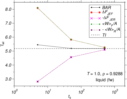
Figure 1: (Color online) Estimates of $\gamma_{\text{wl}}$ for the flat wall (fw) at the indicated values of $T$ and $\rho$ from non-equilibrium work methods (see text). The horizontal dotted line is the result from TI. All results are obtained from an extrapolation to $L_{\rm z}^{-1}=0$. Error bars are not shown as they are less than the symbol size.

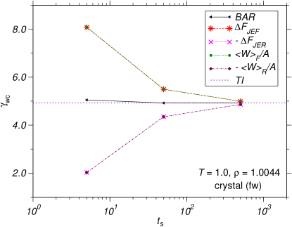
Figure 2: (Color online) $\gamma_{\text{wc}}$ vs. $t_{\rm s}$ at the indicated values of $T$ and $\rho$ obtained using TI and several non-equilibrium work methods. Error bars are less than the symbol size.

We first show results obtained from the four different methods at temperature $T=1.0$ and the coexistence densities $0.9288\,\sigma^{-3}$ and $1.0044\,\sigma^{-3}$ for the liquid and the crystal, respectively. In the following, we denote the estimated interfacial free energy from JE [cf. Eq. (12)] for the forward switching process by $\Delta F_{\rm JEF}$ and that for the negative of the reverse switching process by $-\Delta F_{\rm JER}$. We compare $\Delta F_{\rm JEF}$ and $-\Delta F_{\rm JER}$ to the correspondent average work values (divided by the interface area $A$), $\langle W\rangle_{\rm F}/A$ and $-\langle W\rangle_{\rm R}/A$, respectively. Estimates of $\gamma_{\text{wl}}$ and $\gamma_{\text{wc}}$ from the non-equilibrium work methods as a function of switching time $t_{\rm s}$ are shown in Figs. 1 and 2, respectively. Note that all the results in these figures are obtained from an extrapolation to $L_{z}^{-1}=0$ (see above). Since, $\langle W\rangle_{\rm F}>\Delta F$, it follows that $\langle W\rangle_{\rm R}>-\Delta F$ or $-\langle W\rangle_{\rm R}<\Delta F$. These relations are rationalized by our calculations (see figures).

Figures 1 and 2 show that, as the switching time $t_{\rm s}$ increases, $\Delta F_{\rm JEF}$ and $-\Delta F_{\rm JER}$ gradually converge to the interfacial free energies, as obtained from the TI scheme (horizontal dotted lines). As indicated in the figures, the JE values are similar to the corresponding average work values. Whereas at small switching times ($t_{\rm s}\lesssim 50$) the JE estimates significantly differ from the TI value, for $t_{\rm s}=500$ the deviation between the JE and TI values is less than 2% (this also holds for the corresponding average work values). On the other hand, the free energy estimated by the BAR method is in excellent agreement with the TI value already at $t_{\rm s}=50$, with difference between the two estimates being less than 0.3%. However, at $t_{\rm s}=50$, the error bars corresponding to the BAR method are larger than those of the TI values. Only at $t_{\rm s}=500$, the error bars for the BAR and TI method have the same order of magnitude. Similarly, the magnitude of the error bars corresponding to the JE estimates and the average work values reduce to those of the TI method at $t_{\rm s}=500$.

We find that the BAR method (with $t_{\rm s}=50$) is twice as fast as the TI approach, though, for $t_{\rm s}=50$, the error bars for the BAR method are slightly larger. At $t_{\rm s}=500$, the error bars and also the computational load for the BAR and the TI method are similar and the BAR method is no more computationally advantageous compared to the TI approach. On the other hand, the computational load needed for the JE estimates and the corresponding average work values, at $t_{\rm s}=500$, is about one third that of the TI method, which is still faster compared to the BAR method at the smaller switching time $t_{\rm s}=50$. Since the BAR approach requires information from both the forward and reverse trajectories its efficiency is reduced as compared to the JE estimates, which need calculations only in one direction, either forward or reverse.

The good agreement of the average work values for $t_{\rm s}=500$ with the TI results, shows that at this switching time the switching process is quasi-static and hence is akin to a TI. In our TI simulations, carried out independently of the non-equilibrium work simulations, we choose a much larger equilibration time before the production runs thus increasing the computational load. Hence, an advantage of carrying out simulations with various switching times to calculate the non-equilibrium work, allows us to identify the switching time required for the transformation from the initial to the final state to be quasi-static and reduce to a conventional TI. The good agreement of the average work values with JE estimates at $t_{\rm s}=500$ and with the TI data also indicates that there is no advantage in using the non-equilibrium work method over a TI approach as regards computational speed is concerned. However, carrying out simulations for both forward and reverse switching processes help us to check for any hysteresis in the TI. The convergence of both the forward and reverse work values (divided by $A$) to the interfacial free energy obtained from TI, indicates the lack of hysteresis in our TI scheme. Secondly, the good agreement between the non-equilibrium work and TI method also validates the accuracy of our TI method.

In the remainder of this subsection, unless otherwise indicated, we show results pertaining to the non-equilibrium work approach obtained using only the BAR method for the switching time $t_{\rm s}=500$.

To determine the interfacial free energy along an isotherm at different densities or along a coexistence curve at different temperatures via the GC integration we need as input $\gamma_{\rm wl}$ at one point along the curve as well as the excess volume (in case of determining $\gamma_{\rm wl}$ along the coexistence curve, also the excess energy) at all points along the curve at which $\gamma_{\rm wl}$ is to be determined.

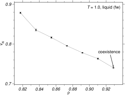
Figure 3: (Color online) Excess interfacial volume $v_{\rm N}$ as a function of density at $T=1.0$, for the liquid in contact with a flat wall (fw).

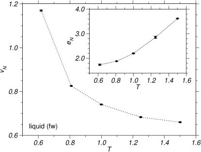
Figure 4: (Color online) Excess interfacial volume $v_{\rm N}$ and (in the inset) excess interfacial energy ($e_{\rm N}$) as a function of the temperature along the liquid-crystal coexistence curve for liquid in contact with a flat wall.

$\begin{array}[]{cc}\includegraphics[width=216.81pt]{fig5a.eps}&\includegraphics[width=216.81pt]{fig5b.eps}\end{array}$

Figure 5: (Color online) Interfacial free energies of the (a) liquid in contact with the flat wall and (b)(111) orientation of the crystal in contact with the flat wall for different system sizes $L_{\rm z}$ of the simulation cell along the $z$ direction at the coexistence temperature $T=1.0$. The coexistence densities of the liquid and crystal at this temperature are $0.9288\sigma^{-3}$ and $1.0044\sigma^{-3}$ respectively. For the wall-liquid interfaces, the interfacial free energy obtained from the PA, GC, TI and BAR methods are shown, while for the wall-crystal simulations, data obtained from the TI and BAR methods are plotted. The straight lines connecting the points denote a linear least-squares fit from whose intercepts the interfacial free energies are determined. In (b) error bars are less than the symbol size.

$\begin{array}[]{cc}\includegraphics[width=216.81pt]{fig6a.eps}&\includegraphics[width=216.81pt]{fig6b.eps}\end{array}$

Figure 6: (Color online) (a) $\gamma_{\text{wl}}$ and $\gamma_{\text{wc}}$ (shown in the inset) as a function of the melting temperature and (b) $\gamma_{\rm wl}$ vs. density of the liquid at $T=1.0$. In (a) two sets of GC data are shown for $\gamma_{\text{wl}}$. One corresponds to data where the initial known value of the interfacial free energy is taken from the TI data at $T=0.618$ and the values for $T>0.618$ obtained via GC integration. The second curve corresponds to the case where the known value of $\gamma_{\text{wl}}$ was taken from the TI data at $T=0.809$ and for $T>0.809$, the interfacial free energies are obtained using GC integration. In case of (b), the known value of $\gamma_{\text{wl}}$ was taken from the TI data at the lowest value of the given liquid density. The data corresponding to the BAR method represent results for a switching time $t_{\rm s}=500.0$. Error bars in (a) and (b) are less than the symbol size.

Figure 3 shows the excess volume as a function of density up to the coexistence density at $T=1.0$. Since the temperature is constant ($dT=0$), the first term in Eq. (14) is zero and we only need the interfacial excess volume, $v_{N}(\rho)$ and one reference value for $\gamma_{\rm wl}$. Here, this reference value was taken from the TI result corresponding to the lowest density at $\rho_{\rm l}=0.811\sigma^{-3}$. Note that the lateral system sizes were kept at $L_{x}=13.5892\sigma$ and $L_{y}=15.691\sigma$ for the different densities. From the lowest to the highest density, the system sizes along the $z$ direction were $66.907\,\sigma$, $65.420\,\sigma$, $63.998\,\sigma$, $62.636\,\sigma$, $61.331\,\sigma$, $69.678\,\sigma$, and $68.285\,\sigma$, respectively. The number of particles for all densities up to $\rho_{\rm l}=0.8916\sigma^{-3}$ was $N=11661$. For $\rho_{\rm l}=0.9102\,\sigma^{-3}$ and $\rho_{\rm l}=0.9288\,\sigma^{-3}$, $N=13524$ was chosen.

The interfacial excess quantities were also computed for all the other system sizes from which the final value of $\gamma_{\rm wl}$ was determined by an extrapolation to $L_{z}^{-1}=0$. At all other system sizes, the interfacial excess quantities had similar values and varied in the same manner along the isotherm at the different densities. There was no clear dependence of the interfacial excess quantities on the system size. As the density increases and approaches the liquid coexistence density at this temperature, $0.9288\,\sigma^{-3}$, the bulk pressures in the liquid also increase. Similar to the hard-sphere case laird09 , we also find that the excess volume decreases with increasing density (or bulk pressure).

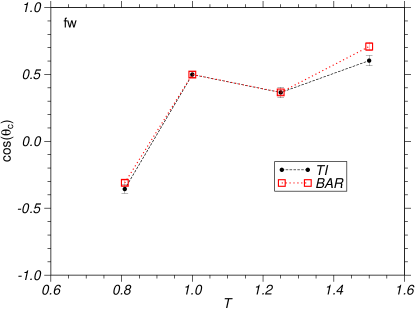
Figure 7: (Color online) Cosine of the contact angle as a function of temperature along liquid-crystal coexistence for system in contact with a flat wall, obtained from Young’s equation by using $\gamma_{\rm wl}$ and $\gamma_{\rm wc}$ from the TI and BAR data of Fig. 6a and using values of $\gamma_{\text{cl}}$ as reported in Ref. davidchack-laird03 . Error bars are less than the symbol size.

Figure 4 shows the excess volume and excess energy as function of temperature at coexistence. The system sizes $L_{x}\times L_{y}\times L_{z}$ corresponding to the different temperatures are as follows: $13.871\times 16.016\times 63.378$ at $T=0.618$, $13.727\times 15.851\times 70.397$ at $T=0.809$, $13.589\times 15.691\times 68.285$ at $T=1.0$, $13.428\times 15.505\times 67.357$ at $T=1.25$, and $13.288\times 15.344\times 66.134$ at $T=1.5$ (with all lengths in units of $\sigma$). The number of particles was $N=11661$ at $T=0.618$ and $N=13524$ at the other temperatures. It is observed that the excess volume decreases with temperature while the excess energy shows an increase with temperature. We note that the interfacial excess quantities do not exhibit finite-size effects for the considered system sizes.

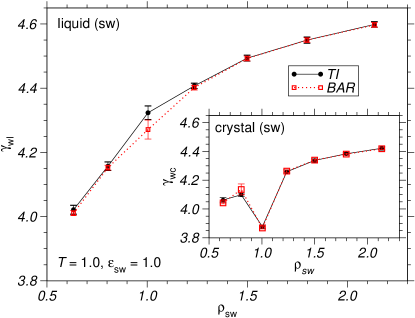
Figure 8: (Color online) $\gamma_{\text{wl}}$ and $\gamma_{\text{wc}}$ (shown in the inset) as function of $\rho_{\rm sw}$ at the temperature $T=1.0$ and $\epsilon_{\rm sw}=1.0$, obtained from the BAR (with $t_{\rm s}=500$) and the TI method.

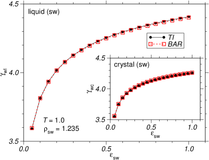
Figure 9: (Color online) $\gamma_{\text{wl}}$ and $\gamma_{\text{wc}}$ (shown in the inset) versus the interaction strength $\epsilon_{\rm sw}$ at the temperature $T=1.0$ and $\rho_{\rm sw}=1.235$ obtained using the BAR (with $t_{\rm s}=50$) and TI methods. Error bars are less than symbol size.

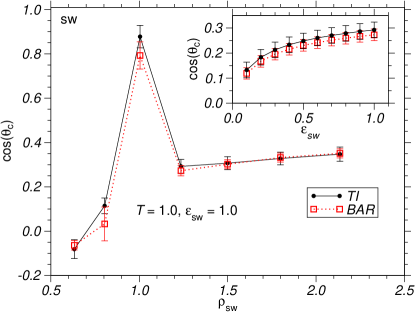
Figure 10: (Color online) Cosine of the contact angle obtained from Young’s equation at the temperature $T=1.0$ as a function of $\rho_{\rm sw}$ at $\epsilon_{\rm sw}=1.0$ and in the inset versus the interaction strength $\epsilon_{\rm sw}$ at $\rho_{\rm sw}=1.235$. $\gamma_{\rm wl}$ and $\gamma_{\rm wc}$ were taken from the BAR and TI data of Figs. 8 and 9 and values of $\gamma_{\rm cl}$ reported in Ref. davidchack-laird03 were used.

For each individual run and system size, the interfacial excess quantities and the GC integration was carried out independently to obtain $\gamma_{\text{wl}}$ along an isotherm as a function of density and along the melting curve as a function of temperature. From the obtained values of $\gamma_{\text{wl}}$ for the four considered system sizes, an extrapolation was performed to $L_{z}^{-1}=0$ and the final values were calculated from the intercepts with the ordinate. In Figs. 5a and 5b, we show the results for the interfacial free energy from the various methods as a function of $1/L_{z}$ for the liquid and crystal in contact with the flat wall, respectively. While the extrapolated values obtained from the BAR, TI and GC methods are in good agreement with each other up to the numerical acccuracy, results obtained from the PA method deviate from the rest by $2-3\%$.

Figure 6a shows $\gamma_{\rm wc}$ and $\gamma_{\text{wl}}$ as a function of temperature along the melting curve, and in Fig. 6b, $\gamma_{\rm wl}$ is displayed as a function of density at $T=1.0$. For the crystal, we find very good agreement between the BAR and the TI methods (inset of Fig. 6). To determine $\gamma_{\rm wl}$ along the melting curve, the interfacial free energy obtained from the TI method at $T=0.618$ was first chosen as the initial value for the GC integration. With this initial value, the agreement of the GC integration data with the TI and BAR data becomes progressively worse with temperature and at $T=1.5$, the difference between GC and TI or BAR result is around $9\%$. However, when the value of $\gamma_{\rm wl}$ obtained from TI at $T=0.809$ is taken as the initial value, the agreement between the different methods is much better. This could be attributed to the fact that the pressure-temperature melting curve for LJ potentials that we consider here is clearly non-linear asano-fuchizaki12 between $T=0.618$ and $T=0.809$ signifying that more data is needed between these two temperatures, whereas it exhibits essentially linear behavior for $T\geq 0.809$.

For the GC simulations to compute $\gamma_{\rm wl}$ along an isotherm at different densities, the interfacial free energy obtained from the TI method at the lowest density was chosen as the initial value to carry out the integration. Figure 6b clearly shows excellent agreement between all the four methods. The error bars corresponding to the different methods are all of a similar magnitude.

From the values for $\gamma_{\rm wl}$ and $\gamma_{\rm wc}$ predicted by the BAR and TI methods and using the data from Ref. davidchack-laird03 for $\gamma_{\rm cl}$, we determined the cosine of the contact angle as a function of temperature along the coexistence curve via Young’s equation. The results are shown in Fig. 7. At $T=0.618$, $(\gamma_{\text{wl}}-\gamma_{\text{wc}})/\gamma_{\text{cl}}<-1$, corresponding to the complete drying conditions. As $T$ increases, the flat wall prefers the crystal more than the liquid ($\gamma_{\rm wc}<\gamma_{\rm wl}$) and incomplete wetting is observed ($-1<\cos\theta_{\rm c}<1$). At higher temperatures ($T>1.0$) partial wetting is observed ($0<\cos\theta_{\rm c}<1$), with $\cos\theta_{\rm c}$ varying non-monotonically with respect to temperature along the melting curve. While good agreement is found in general between the BAR and TI methods, here, we observe a slightly larger difference between them as compared to that for the individual interfacial free energies. This is because $\cos\theta_{\rm c}$ depends on the difference between $\gamma_{\text{wl}}$ and $\gamma_{\text{wc}}$, which magnifies the relative error.

IV.2 Structured Wall

We now consider the LJ system in contact with a structured wall, with the interaction between the wall and the LJ system to be of the same purely repulsive WCA potential. For the structured wall, the interesting parameters are the interaction strength and the density of the wall. We study the variation of the interfacial free energy as a function of these two parameters at the liquid-crystal coexistence temperature $T=1.0$, choosing the coexistence densities $0.9288\,\sigma^{-3}$ and $1.0044\,\sigma^{-3}$ for the liquid and the crystal, respectively. In the following the BAR and the TI method are compared.

In Fig. 8, we plot the interfacial free energies of the LJ liquid and crystal as a function of the density of the wall (at $\epsilon_{\rm sw}=1.0$). In the computations with the BAR method a switching time of $t_{\rm s}=500$ was used. The density of the structured wall was modified by choosing different lattice constants for the fcc structure of the wall. We observe that the interfacial free energy of the liquid increases with increasing density of the wall. Increasing density of the wall means a larger repulsive force acting on the liquid particles which enhances $\gamma_{\text{wl}}$. The general trend for $\gamma_{\text{wc}}$ is the same. However, when the density of the wall is the same as the equilibrium density of the crystal we find a sharp dip in the interfacial free energy. This is expected since when the wall has the same structure as the crystal less energy is required to create an interface.

Figure 9 shows $\gamma_{\rm wl}$ and $\gamma_{\rm ws}$ for different interaction strengths $\epsilon_{\rm sw}$ between the wall and the LJ system. The density of the substrate is $\rho_{\text{sw}}=1.235$, i.e. the density of the structured wall is larger than that of the bulk LJ crystal. To reduce the computational effort, $\epsilon_{\rm sw}$ was itself used as the switching parameter, with the system at $\epsilon_{\rm sw}=1$ considered as the reference state. For the BAR calculations, a switching time $t_{\rm s}=50$ was sufficient to obtain good agreement with the TI method as regards the mean value and also the standard deviation. All the data corresponding to the BAR calculations in Fig. 9 are shown for a switching time $t_{\rm s}=50$. Increasing the interaction strength between the wall and the LJ system leads to a greater repulsive interaction between them, thereby enhancing the interfacial free energies.

As can be inferred from Figs. 8 and 9, at the considered thermodynamic states $\gamma_{\rm wc}<\gamma_{\rm wl}$ holds. This signifies the occurrence of incomplete wetting. To determine the contact angle from Young’s equation, we use $\gamma_{\rm cl}$, as obtained by the cleaving potential method laird10 , and $\gamma_{\rm wl}$ and $\gamma_{\rm wc}$, as estimated by our TI scheme and the BAR method. Figure 10 shows that cosine of the contact angle increases with the density of the structured wall, with a sharp peak when the density of the wall is equal to the average density of the bulk crystal. At this value of the wall density, we found that the corresponding contact angle reaches a minimum and is about $25^{\circ}$, which is in the partial wetting regime. Contact angles are less than $90^{\circ}$ ($0<\cos\theta_{\rm c}<1$) at all wall densities except at the smallest $\rho_{\text{sw}}$ since there $\gamma_{\text{wc}}>\gamma_{\text{wl}}$ (see Fig. 8).

Figure 10 also shows $\cos\theta_{\rm c}$ increasing with increasing interaction strength between the the wall and the LJ system. This is because $\gamma_{\rm wl}$ and $\gamma_{\rm wc}$ gradually diverge from each other as $\epsilon_{\rm sw}$ increases, as is clearly seen in Fig. 9. $0<\cos\theta_{\rm c}<1$ at all values of $\epsilon_{\rm sw}$ indicating that the LJ crystal partially wets the wall for such parameter values.

V Conclusion

In this work, extensive MD simulations of a LJ system were performed to compare different techniques for the calculation of wall-liquid and wall-crystal interfacial free energies. We find that the equilibrium thermodynamic integration (TI) method is in very good agreement with non-equilibrium work techniques such as the Bennett acceptance ratio (BAR) method. Within the restricted range of applicalbility, this also holds for Gibbs-Cahn (GC) integration and the pressure anisotropy (PI) method. This indicates the accuracy of the obtained estimates and also validates the TI scheme, proposed in our earlier work.

While the GC method is computationally faster compared to the TI or BAR methods, care has to be taken when the coexistence pressure and temperature vary non-linearly along the melting curve since then more number of points are needed to obtain reliable values for the interfacial free energy. As a matter of fact, non-equilibrium work methods are not more efficient compared to conventional TI. However, such methods are helpful to check for any hysteresis in the TI scheme.

Using the obtained values of $\gamma_{\rm wl}$ and $\gamma_{\rm wc}$ and the values for $\gamma_{\rm cl}$ calculated previously using the “cleaving potential method” davidchack-laird03 , we applied Young’s equation to determine contact angles for flat and structured walls. In general, one observes smaller contact angles at higher temperatures along the melting curve when the LJ system is in contact with the flat wall. For the structured wall interfaces, it is found that the density of the structured wall and the interaction strength of the LJ particles with the wall significantly influence the contact angle and the degree of wetting can be changed by tuning such parameters. In particular, the contact angle exhibits a strongly non-monotonic behavior with respect to the density of the structured wall, as it shows a sharp minima when the density of the structured wall is equal to that of the bulk crystal.

Both for the flat and the structured walls we have obtained the conditions under which partial wetting is observed. Thus, the models proposed in this work can now be used for the study of heterogeneous nucleation.

- (1) P. G. de Gennes, Rev. Mod. Phys. 57, 827 (1985); P. G. de Gennes, F. Brochart-Wyart, and D. Quéré, Capillarity and Wetting Phenomena. Drops, Bubbles, Pearls, Waves (Springer, New York, 2004).
- (2) A. C. Zettlemoyer (ed), Nucleation (New York: Dekker, 1969).
- (3) F. F. Abraham, Homogeneous Nucleation Theory (New York: Academic, 1974).
- (4) D. Kashchiev, Nucleation: Basic Theory with Applications (Oxford: Butterworth-Heinemann, 2000).
- (5) A. W. Adamson and A. P. Gast, Physical chemistry of surfaces (Wiley-Interscience, New York, 1997).
- (6) G. Navascués, Rep. Prog. Phys. 42, 1131 (1979).
- (7) J. M. Howe, Interfaces in Materials (Wiley, New York, 1997); M. E. Glicksman and N. B. Singh, J. Cryst. Growth 98, 277 (1989); M. Muschol, D. Liu, and H. Z. Cummins, Phys. Rev. A 46, 1038 (1992).
- (8) M. P. Allen and D. J. Tildesley, Computer Simulations of Liquids (Clarendon, Oxford, 1987).
- (9) D. P. Landau and K. Binder, A Guide to Monte Carlo Simulations in Statistical Physics (Cambridge, USA, 2000).
- (10) D. Frenkel and B. Smit, Understanding Molecular Simulation (Academic, San Diego, 2002); T. P. Straatsma, M. Zacharias, and J. A. MacCammon, Computer Simulations of Biomolecular Systems (Escom, Keiden, 1993).
- (11) J. G. Kirkwood and F. P. Buff, J. Chem. Phys. 17, 338 (1949).
- (12) J. R. Henderson and F. van Swol, Mol. Phys. 51, 991 (1984).
- (13) D. J. Courtemanche, T. A. Pasmore and F. van Swol, Mol. Phys. 80, 861 (1993).
- (14) E. De Miguel and G. Jackson, Mol. Phys. 104, 3717 (2006).
- (15) J. H. Sikkenk, J. M. J. van Leeuwen, J. O. Indekeu, J. M. J. van Leeuwen, E. O. Vossnack, and A. F. Bakker, J. Stat. Phys. 52, 23 (1988).
- (16) M. J. P. Nijmeijer, C. Bruin, A. F. Bakker, and J. M. J. Van Leeuwen, Physica A 160, 166 (1989).
- (17) M. J. P. Nijmeijer, C. Bruin, A. F. Bakker, and J. M. J. van Leeuwen, Phys. Rev. A 42, 6052 (1990).
- (18) M. J. P. Nijmeijer, C. Bruin, A. F. Bakker, and J. M. J. van Leeuwen, J. Phys.: Condens. Matter 4, 15 (1991).
- (19) M. J. P. Nijmeijer and C. Bruin, J. Chem. Phys. 103, 8201 (1995); C. Bruin, M. J. P. Nijmeijer, and R. M. Crevecoeur, J. Chem. Phys. 102, 7622 (1995).
- (20) J. Z. Tang and J. G. Harris, J. Chem. Phys. 103, 8201 (1995); J. G. Harris, J. Chem. Phys. 105, 4889 (1996).
- (21) F. Varnik, J. Baschnagel, and K. Binder, J. Chem. Phys. 113, 4444 (2000).
- (22) R. Shuttleworth, Proc. Phys. Soc. A 63, 444 (1950).
- (23) B. B. Laird and R. L. Davidchack, J. Chem. Phys. 132, 204101 (2010).
- (24) W. A. Tiller, The Science of Crystallization: Microscopic Interfacial Phenomena (Cambridge Univ. Press, New York, 1991).
- (25) D. Deb, A. Winkler, M. H. Yamani, M. Oettel, P. Virnau, and K. Binder, J. Chem. Phys. 134, 214706 (2011).
- (26) D. Deb, D. Wilms, A. Winkler, P. Virnau, and K. Binder, Int. J. Mod. Phys. C (2012).
- (27) F. Leroy, Daniel J. V. A. dos Santos, and F. Müller-Plathe, Macromol. Rapid Commun. 30, 864 (2009); F. Leroy and F. Müller-Plathe, J. Chem. Phys. 133, 044110 (2010).
- (28) M. Heni and H. Löwen, Phys. Rev. E 60, 7057 (1999).
- (29) A. Fortini and M. Dijkstra, J. Phys.: Condens. Matter 2006, 18, L371.
- (30) B. B. Laird and R. L. Davidchack, J. Phys. Chem. C 111, 15952 (2007).
- (31) R. Benjamin and J. Horbach, J. Chem. Phys. 137, 044707 (2012).
- (32) C. Jarzynski, Phys. Rev. Lett. 78, 2690 (1997).
- (33) C. Jarzynski, Phys. Rev. E 73, 046105 (2006).
- (34) R. F. Fox, Proc. Natl. Acad. Sci. USA 100, 12537 (2003).
- (35) M. R. Shirts and V. S. Pande, J. Chem. Phys. 122, 144107 (2005).
- (36) C. H. Bennett, J. Comput. Phys. 22, 245 (1976).
- (37) Y. Mu and X. Song, J. Chem. Phys. 124, 034712 (2006).
- (38) R. L. Davidchack, J. Chem. Phys. 133, 234701 (2010).
- (39) B. B. Laird, R. L. Davidchack, Y. Yang, and M. Asta, J. Chem. Phys. 131, 114110 (2009).
- (40) J. W. Cahn, in Interfacial Segregation, Ed.:W C. Johnson and J. M. Blakeley (American Society for Metals, Metals Park, OH, 1979), pp. 3-23.
- (41) J. W. Gibbs, The Collected Works (Yale University Press, New Haven, CT, 1957), Vol. 1.
- (42) T. Young, Phil. Trans. R. Soc. 95, 65 (1805).
- (43) J. Q. Broughton and G. H. Gilmer, J. Chem. Phys. 84, 5759 (1986).
- (44) R. L. Davidchack and B. B. Laird, J. Chem. Phys. 118, 7651 (2003).
- (45) Y. Asano and K. Fuchizaki, J. Chem. Phys. 137, 174502 (2012).
- (46) Y. Asano and K. Fuchizaki, J. Phys. Soc. Jpn. 78, 055002 (2009).
- (47) W. H. Press, B. P. Flannery, S. A. Teukolsky, and W. T. Vetterling, Numerical Recipes in FORTRAN, 2nd ed. (Cambridge University Press, Cambridge, U.K., 1992).
- (48) T. Frolov and Y. Mishin, Phys. Rev. B 79, 045430 (2009).
- (49) T. Frolov and Y. Mishin, J. Chem. Phys. 131, 054702 (2009).
- (50) S. Kim, Y. W. Kim, P. Talkner, and J. Yi, Phys. Rev E 86, 041130 (2012).