A long-term VLBA monitoring campaign of the SiO masers toward TX Cam
I. Morphology and Shock Waves

Abstract

We present the latest and final version of the movie of the SiO masers toward the Mira variable TX Cam. The new version consists of 112 frames (78 successfully reduced epochs) with data covering almost three complete stellar cycles between 24^th May 1997 and 25^th January 2002, observed with the VLBA. In this paper we examine the global morphology, kinematics and variability of the masering zone. The morphology of the emission is confined in a structure that usually resembles a ring or an ellipse, with occasional deviations due to localised phenomena. The ring appears to be contracting and expanding, although for the first cycle contraction is not observed. The width and outer boundary of the masering zone follow the stellar pulsation. Our data seem to be consistent with a shock being created once per stellar cycle at maximum that propagates with a velocity of $\sim$7 km s^-1. The difference in velocities along different axes strongly suggests that the outflow in TX Cam is bipolar. The contribution of projection is examined and our results are compared with the latest theoretical model.

1 Introduction

The discovery of pulsating variability in stars can be traced back to 1596, when David Fabricius (Wolf 1877) first observed the phenomenon in an individual star that later would give its name to an entire variability class. Johann Fokkens Holwarda in his book Historiola Mirae Stellae named the star Mira, the latin world for Wonderful (Poggendorff 1863). We now know that these “Wonderful” Variables are evolved red giants, located on the Asymtotic Giant Branch (AGB) of the H-R diagram. Mira Variables mark a stage in the evolutionary path of stars with zero age main sequence masses between of 1$<M_{\sun}<$8 that pulsate with regular periodicity and have fluctuation in the V-band greater than 2.5^m (Habing 1996; Habing & Olofsson 2004). Regarding the structure of typical Miras, they have a radius of 2 AU or more and they consist of a degenerated C/O core, surrounded by a thin layer of helium, that is in turn covered by a huge hydrogen mantle (Habing 1996). Due to their high mass-loss rates (10^-7 to 10^-4 M_☉) they are surrounded by an extended Circumstellar Envelope (CSE) (Olofsson 2001). The near-circumstellar morphology is not necessarily symmetric however (Josselin et al. 2000; Thomson, Creech-Eakman & Akeson 2002). Observations with the Infrared Optical telescope Array by Ragland et al. (2006) show that one third of the Miras in their sample were found to have significant asymmetries.

The total luminosity of Miras vary by only approximately an order of magnitude; However, in the visual part of the spectrum they can vary by up to 8 orders of magnitude. Their relatively low photospheric surface temperatures (2000-3500 K) allow the formation of molecules in their CSEs during minima, including metalic oxides which absorb wide bands of the optical spectrum, resulting in the extreme visual variabilty observed (Reid & Goldston 2002).

SiO masers are located between the dust formation region and the stellar atmosphere (Elitzur 1992), in a very complex area known as the extended atmosphere. Wittkowski et al. (2007) conducted the first multi-epoch mid-infrared and radio interferometry study of a Mira star (S Ori), in order to determine the photospheric radius, the dust shell parameters and the SiO maser spot location and examine dependences on the pulsation phase. They concluded that, during minimum visual phase, dust (consisting only of Al₂O₃) and SiO masers are co-located, forming close to the surface. However, after the visual maximum, the inner dust shell is expanded by $\sim 20\%$ while the maser spots remain at about the same location.

The first high resolution images of the 43 GHz SiO masers around late-type stars were produced by Miyoshi et al. (1994), Diamond et al. (1994) and Greenhill et al. (1995) and revealed that the masers are confined to well defined projected rings, overruling the prevailing belief at that time that SiO masers form chaotic structures around variable stars. The VLBA observations of the Miras TX Cam and U Her by Diamond et al. (1994) showed that SiO masers form at 2-4 R_⋆, placing them in the extended atmosphere of the stars, inside the dust formation zone. The main kinematic behaviour appeared to be that of outflow. The emission pattern was consistent with tangential amplification. Subsequent to these initial reported observations, a synoptic monitoring campaign was commenced for a limited number of sources.

The first movie of the TX Cam monitoring campaign was published by Diamond & Kemball (2003). This paper included the first 41 epochs as a movie of 44 frames covering a complete stellar pulsation cycle at an angular resolution of $\sim$0.1 mas and revealed the gross kinematic properties of the SiO maser emission. The morphology and properties of the shell varied with time and stellar phase. Individual maser features persisted over many epochs and the predominant kinematic behaviour of the ring was that of expansion. Contrary to the models that assume spherical symmetry, the structure and evolution of the ring revealed a high degree of asymmetry. There was also evidence of ballistic deceleration and proper motion analysis revealed motions between $\sim$5-10 km s^-1, distributed around the ring.

An expanded 73-frame movie (60 epochs) by Gonidakis et al. (2010) uncovered more properties of the morphology and the kinematics of the masering shell. Over two pulsation cycles, the movie revealed that contraction occurred during the second cycle. The time-span of the movie allowed the study of short- and long-term variability properties, i.e. changes not only within a cycle but also from one cycle to another. The 43 GHz flux variability was found to follow that of the optical with a $\sim$10% lag but the flux densities were uncorrelated. The width of the ring was also found to be correlated with the stellar pulsation phase but there was no correlation found between the velocities and position angle of the ring. The lifetime of individual components were found to follow a Gaussian distribution with a peak between 150 and 200 days, while the spectra were dominated by blue and red-shifted peaks that formed at different times in the stellar cycle and had different lifetimes.

The paper is organised as follows. Section 2 outlines the observations and data reduction. In Section 3 the new version of the movie is presented, as well as the analysis of the data and the results. Section 4 examines the contribution of shock waves to the overall structure and kinematics. The science results are discussed in Section 5 and the paper ends with the conclusions of this study in Section 6.

2 Observations and data reduction

The monitoring of the masers on TX Cam started on the 24^th of May 1997 with the Very Long Baseline Array (VLBA), and one antenna from the VLA. Until the 9^th of September 1999, observations were conducted in biweekly intervals. From that date until the end of the project on the 25^th of January 2002, the intervals were monthly. Given a pulsation period of 557 days for TX Cam (Kholopov et al. 1985) they correspond to a coverage of 3.06 pulsation periods. The result was 82 individual datasets, 78 of which were reduced successfully. Due to bad weather conditions over parts of the array or loss of crucial antennae near the array centre, some epochs did not produce images of acceptable quality and had to be discarded.

All epochs were observed at a rest frequency of 43.122027 GHz, centred at an LSR velocity of 9.0 km s^-1. Each observing run was 6-8 hours long, with 2.5-3.5 hours devoted to TX Cam and the rest to calibrators and other target sources. Data were recorded in dual polarisation over a 4 MHz bandwidth and correlated with the VLBA correlator in Socorro, creating datasets in all 4 cross-polarisation pairs over 128 spectral channels. The nominal spectral resolution was 31.25 kHz, corresponding to a velocity resolution of 0.217 km s^-1.

The science goals of the project required consistency and uniformity in both observations and data analysis. A uniform observing strategy was assured by retaining the same configuration during each experiment as described in the previous paragraph. The requirement for consistent, uniform data analysis demanded the creation of an automated data reduction procedure. This was developed as a POPS script within the AIPS package and was based on the techniques described by Kemball, Diamond and Cotton (1995) and Kemball and Diamond (1997). The pipeline was divided into logical steps that demanded a minimum of user interaction; this was limited to the examination of the results at the end of each step for quality assurance and the interactive data editing. The final pipeline result for each epoch was a 128-channel cube of 1024$\times$1024 pixels in Stokes {I,Q,U,V} on the projected plane of the sky with a pixel separation of 0.1 mas.

3 The SiO Masers

3.1 The Movie

One of the objectives of this project was to create a movie to serve as a realistic visualisation of the evolution and distribution of the SiO masers around TX Cam. The final version of the movie consists of 112 frames and covers 3.06 stellar cycles. It would be useful to distinguish between epochs and frames, since these terms will be frequently used in the following paragraphs. The term epoch corresponds to maps produced by actual observations while the term frame includes also the interpolated maps. Thus, the whole project consists of 82 epochs, 78 of which were successfully reduced, 34 interpolated frames due to bad or missing data, resulting into a 112-frame movie.

3.1.1 Post-production

As discussed in the previous section, the data were recorded and reduced identically in order to ensure homogeneity. Further, uniform image post-processing is required in order to render a successful movie visualisation of the maser morphological evolution.The final cubes were averaged over frequency using task SQASH in AIPS giving the final total intensity image for each epoch. In order to suppress spurious features in the noise floor and in order to increase contrast, a cutoff level was applied with task BLANK in AIPS and each frame was converted into its square root with task MATHS. This conversion was only applied to the frames used for the compilation of the movie; for the data analysis the total intensity maps were used. The extent of the maser emission from the circumstellar shell occupied only a sub-region within each 1024$\times$1024 pixel frame, so the final image processing step was to trim them down to 680$\times$680 pixels using task SUBIM.

Table 1: List of epochs, observation dates and the corresponding phase of the star. Comments in the status column indicate missing or failed epochs. These epochs were interpolated in order to have a smooth, time coherent movie. The time when observations switched to a monthly interval is indicated in the table.

Epoch code	Observing date	Optical phase	Status	Epoch code	Observing date	Optical phase	Status
Observations every 2 weeks				Observations every month
BD46A	1997 May 24	0.68 $\pm$ 0.01	$\surd$	BD62A	1999 September 9	2.18 $\pm$ 0.01	$\surd$
BD46B	1997 June 7	0.70 $\pm$ 0.01	$\surd$	BD62AB	1999 September 27	2.21 $\pm$ 0.01	$\between$
BD46C	1997 June 22	0.73 $\pm$ 0.01	$\surd$	BD62B	1999 October 15	2.24 $\pm$ 0.01	$\times$
BD46D	1997 July 6	0.75 $\pm$ 0.01	$\surd$	BD62BC	1999 October 31	2.27 $\pm$ 0.01	$\between$
BD46E	1997 June 19	0.78 $\pm$ 0.01	$\surd$	BD62C	1999 November 14	2.30 $\pm$ 0.01	$\surd$
BD46F	1997 August 2	0.80 $\pm$ 0.01	$\surd$	BD62CD	1999 December 2	2.33 $\pm$ 0.01	$\between$
BD46G	1997 August 16	0.83 $\pm$ 0.01	$\surd$	BD62D	1999 December 19	2.36 $\pm$ 0.01	$\surd$
BD46H	1997 August 28	0.85 $\pm$ 0.01	$\surd$	BD62DE	2000 January 1	2.38 $\pm$ 0.01	$\between$
BD46I	1997 September 12	0.87 $\pm$ 0.01	$\surd$	BD62E	2000 January 15	2.41 $\pm$ 0.01	$\surd$
BD46J	1997 September 26	0.90 $\pm$ 0.01	$\surd$	BD62EF	2000 January 31	2.44 $\pm$ 0.01	$\between$
BD46K	1997 October 9	0.92 $\pm$ 0.01	$\surd$	BD62F	2000 February 14	2.46 $\pm$ 0.01	$\surd$
BD46L	1997 October 25	0.95 $\pm$ 0.01	$\times$	BD62FG	2000 March 2	2.49 $\pm$ 0.01	$\between$
BD46M	1997 November 8	0.98 $\pm$ 0.01	$\surd$	BD62G	2000 March 17	2.52 $\pm$ 0.01	$\surd$
BD46N	1997 November 21	1.00 $\pm$ 0.01	$\surd$	BD62GH	2000 April 4	2.55 $\pm$ 0.01	$\between$
BD46O	1997 December 5	1.03 $\pm$ 0.01	$\surd$	BD62H	2000 April 21	2.58 $\pm$ 0.01	$\surd$
BD46P	1997 December 17	1.05 $\pm$ 0.01	$\surd$	BD62HI	2000 May 5	2.61 $\pm$ 0.01	$\between$
BD46Q	1997 December 30	1.07 $\pm$ 0.01	$\times$	BD62I	2000 May 21	2.64 $\pm$ 0.01	$\surd$
BD46R	1998 January 13	1.10 $\pm$ 0.01	$\surd$	BD62IA	2000 June 6	2.67 $\pm$ 0.01	$\between$
BD46S	1998 January 25	1.12 $\pm$ 0.01	$\surd$	BD69A	2000 June 22	2.70 $\pm$ 0.01	$\surd$
BD46T	1998 February 5	1.14 $\pm$ 0.01	$\surd$	BD69AB	2000 July 4	2.72 $\pm$ 0.01	$\between$
BD46U	1998 February 22	1.17 $\pm$ 0.01	$\surd$	BD69B	2000 July 16	2.74 $\pm$ 0.01	$\surd$
BD46V	1998 March 5	1.19 $\pm$ 0.01	$\surd$	BD69BC	2000 August 3	2.77 $\pm$ 0.01	$\between$
BD46VW	1998 March 21	1.22 $\pm$ 0.01	$\between$	BD69C	2000 August 21	2.81 $\pm$ 0.01	$\times$
BD46W	1998 April 7	1.24 $\pm$ 0.01	$\surd$	BD69CD	2000 September 6	2.84 $\pm$ 0.01	$\between$
BD46X	1998 April 19	1.27 $\pm$ 0.01	$\surd$	BD69D	2000 September 21	2.86 $\pm$ 0.01	$\surd$
BD46Z	1998 May 10	1.30 $\pm$ 0.01	$\surd$	BD69DE	2000 October 5	2.89 $\pm$ 0.01	$\between$
BD46AA	1998 May 22	1.33 $\pm$ 0.01	$\surd$	BD69E	2000 October 19	2.91 $\pm$ 0.01	$\surd$
BD46AB	1998 June 6	1.35 $\pm$ 0.01	$\surd$	BD69EF	2000 November 2	2.94 $\pm$ 0.01	$\between$
BD46AC	1998 June 18	1.37 $\pm$ 0.01	$\surd$	BD69F	2000 November 17	2.96 $\pm$ 0.01	$\surd$
BD46AD	1998 July 3	1.40 $\pm$ 0.01	$\surd$	BD69FG	2000 December 3	2.99 $\pm$ 0.01	$\between$
BD46AE	1998 July 23	1.44 $\pm$ 0.01	$\surd$	BD69G	2000 December 20	3.02 $\pm$ 0.01	$\surd$
BD46AF	1998 August 9	1.47 $\pm$ 0.01	$\surd$	BD69GH	2001 January 1	3.05 $\pm$ 0.01	$\between$
BD46AG	1998 August 23	1.49 $\pm$ 0.01	$\surd$	BD69H	2001 January 20	3.08 $\pm$ 0.01	$\surd$
BD46AH	1998 September 9	1.52 $\pm$ 0.01	$\surd$	BD69HI	2001 February 3	3.10 $\pm$ 0.01	$\between$
BD46AI	1998 September 25	1.55 $\pm$ 0.01	$\surd$	BD69I	2001 February 18	3.13 $\pm$ 0.01	$\surd$
BD46AJ	1998 October 14	1.59 $\pm$ 0.01	$\surd$	BD69IJ	2001 March 3	3.15 $\pm$ 0.01	$\between$
BD46AK	1998 October 29	1.61 $\pm$ 0.01	$\surd$	BD69J	2001 March 16	3.18 $\pm$ 0.01	$\surd$
BD46AL	1998 November 17	1.65 $\pm$ 0.01	$\surd$	BD69JK	2001 March 31	3.20 $\pm$ 0.01	$\between$
BD46AM	1998 December 6	1.68 $\pm$ 0.01	$\surd$	BD69K	2001 April 15	3.23 $\pm$ 0.01	$\surd$
BD46AN	1998 December 23	1.71 $\pm$ 0.01	$\surd$	BD69KL	2001 May 2	3.26 $\pm$ 0.01	$\between$
BD46AO	1999 January 5	1.74 $\pm$ 0.01	$\surd$	BD69L	2001 May 19	3.29 $\pm$ 0.01	$\surd$
BD46AP	1999 January 23	1.77 $\pm$ 0.01	$\surd$	BD69LM	2001 June 6	3.32 $\pm$ 0.01	$\between$
BD46AQ	1999 February 6	1.79 $\pm$ 0.01	$\surd$	BD69M	2001 June 24	3.36 $\pm$ 0.01	$\surd$
BD46AR	1999 February 19	1.82 $\pm$ 0.01	$\surd$	BD69MMN	2001 July 7	3.38 $\pm$ 0.01	$\between$
BD57A	1999 March 12	1.85 $\pm$ 0.01	$\surd$	BD69MN	2001 July 20	3.40 $\pm$ 0.01	$\between$
BD57B	1999 March 29	1.88 $\pm$ 0.01	$\times$	BD69MNN	2001 August 3	3.43 $\pm$ 0.01	$\between$
BD57C	1999 April 12	1.91 $\pm$ 0.01	$\surd$	BD69N	2001 August 16	3.45 $\pm$ 0.01	$\surd$
BD57D	1999 April 24	1.93 $\pm$ 0.01	$\surd$	BD69NA	2001 September 7	3.49 $\pm$ 0.01	$\between$
BD57E	1999 May 14	1.97 $\pm$ 0.01	$\surd$	BD79A	2001 September 28	3.53 $\pm$ 0.01	$\surd$
BD57F	1999 May 31	2.00 $\pm$ 0.01	$\surd$	BD79B	2001 October 12	3.55 $\pm$ 0.01	$\surd$
BD57G	1999 June 12	2.02 $\pm$ 0.01	$\surd$	BD79BC	2001 October 27	3.58 $\pm$ 0.01	$\between$
BD57H	1999 June 27	2.05 $\pm$ 0.01	$\surd$	BD79C	2001 November 12	3.61 $\pm$ 0.01	$\surd$
BD57I	1999 July 12	2.07 $\pm$ 0.01	$\surd$	BD79CD	2001 December 1	3.64 $\pm$ 0.01	$\between$
BD57J	1999 July 30	2.11 $\pm$ 0.01	$\surd$	BD79D	2001 December 18	3.67 $\pm$ 0.01	$\surd$
BD57K	1999 August 11	2.13 $\pm$ 0.01	$\surd$	BD79DE	2002 January 6	3.71 $\pm$ 0.01	$\between$
BD57L	1999 August 24	2.15 $\pm$ 0.01	$\surd$	BD79E	2002 January 25	3.74 $\pm$ 0.01	$\surd$

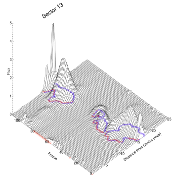
(a)

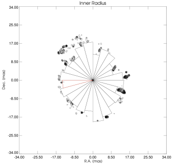
(b)

Figure 1: (a) An example of the technique used for the determination of the inner shell boundary for Sector 13. The surface plot is the concatenation of all the radial intensity profiles over time. The blue contours trace the point with brightness three time that of the off-source regions and the red superimposed crosses correspond to the estimated inner boundary. (b) Total intensity image for frame 55 with the 24 sectors over-plotted as triangles with their apex at the centre of the image and height equal to the calculated radius for each sector. Sector 13 is plotted with red color.

However, the above image processing steps leave two additional unsolved problems, namely the lack of spatial registration between successive frames and non-uniform time sampling over the time series of epochs. The first issue arises from the fact that any information on the absolute position is lost during self-calibration. The second is caused by the switch from biweekly to monthly observing intervals and arises also from epochs with missing data, creating gaps in the movie. These spatial and temporal alignment issues were overcome by developing appropriate software. Each pair of consecutive epochs was first superimposed by eye to establish an approximate shift that should be applied to the second image, in order to register it with the first. After this initial alignment, sub-pixel corrections were calculated using task LGEOM in AIPS (adapted from a program written by Craig Walker). All the corrections were applied using task LGEOM in AIPS. A detailed explanation of the alignment technique can be found at Diamond & Kemball (2003).

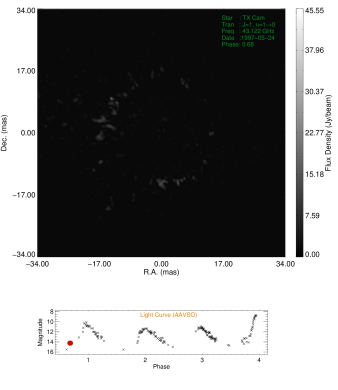
(a)

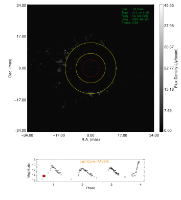
(b)

Figure 7: (a) The first frame of the 112-frame movie, showing the evolution and global kinematics of the SiO masers toward TX Cam. The lower panel is the optical light curve, provided by AAVSO. The red dot follows the phase. (b) Same as in Fig. 7a, but with the addition of the proposed shock (yellow circles) and the pulsating star (red circle). Both movies are provided as online supplementary material.

After the completion of the spatial alignment, the final image processing step was to populate the movie with the missing frames and interpolate it, where needed, onto a regularly spaced set of time intervals. For this purpose we used task COMB in AIPS, to interpolate missing frames as the average of adjacent frames. The frames were concatenated into movie files (in .mov video format) with ffmpeg, a free program for handling multimedia data. Table 1 lists all the frames used to the compilation of this movie into two sets of four columns. In each set, the first column provides the code name for each epoch, the second the date of observation, the third the corresponding phase, calculated from the optical maximum provided by Gray et al. (1999) and the fourth indicates whether the epoch was observed and if it was reduced successfully. The result was a 112-frame movie, covering 3.06 pulsation cycles of TX Cam, the first frame of which can be viewed at Fig. 7a. The movie is provided as online supplementary material of this paper.

3.1.2 The New Release

Structure: As reported in the previous TX Cam studies published (Diamond et al. (1994), Diamond & Kemball (2003) and Gonidakis et al. (2010)) the emission is confined in a projected ring-like structure. Although predominantly circular, the ring can change its shape with time, resembling at times an ellipse, an arc, or even a complicated figure-eight structure. The width of the ring changes with time as does the radius at which it is located relative to its host star. There are three distinct ways for the emission to manifest itself; in elongated filaments, in smaller and more circular spots and in faint diffuse emission. The first two are most common in the inner portion of the ring while diffuse emission is dominant in its outermost parts, defining an abstract outer boundary. The lack of emission within the ring indicates that the amplification of the masers is tangential (Diamond et al. 1994).
Kinematics: The projected ring radius changes with time and significant individual proper motions are apparent. Generally, the flow of the material appears ordered, mainly revealing expansion or contraction, there are though localised deviations from this behaviour. A closer examination reveals mainly four discrete apparent kinematic motions, outflows, inflows, ricochets (features that bounce and change their trajectories, contrary to the ordered kinematic behaviour of their surroundings), and splits (parts of the ring that split into two new arcs, one following the overall motion of the ring and the other moving to the opposite direction). The first two are global, lasting for long fractions of the pulsation period. The latter are rare and localised but they are major contributors in forming the overall shape of the emission.

(a)

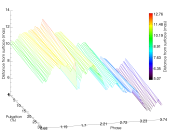
(b)

(c)

Figure 2: (a) The inner shell radius plotted as a function of stellar pulsation. (b) The distance of the inner boundary from the surface of the star for different pulsation amplitudes (see text for adopted stellar radius and pulsation profile). (c) The sector-averaged intensity of the ring plotted with radius.

(a)

(b)

(c)

Figure 3: (a) The average width of the ring plotted as a function of stellar pulsation. (b) The width plotted against inner shell radius. (c) The width plotted against sector-averaged intensity.

3.1.3 Morphological Evolution

The movie is 3.06 periods long but it is spread over 4 stellar cycles, from $\phi$=0.68 to $\phi$=3.74. For convenience in the delineation of the movie, we divide it into four parts, each covering an individual stellar cycle. Features of interest (maser spots, either individual or in groups, with behaviour that deviates from the overall kinematic behaviour) are given a name to make it easier to follow them, especially if they participate in more than one cycle.
Cycle 1 ($\phi$=0.64-1.00): The emission traces the perimeter of a circle but with an obvious gap in the SE and a very weak NW quadrant that by $\phi$=1.00 becomes almost totally void of emission. The E and S sectors start as, and remain, the brightest sections of the ring. The emission is mainly confined in spots and filaments; however, diffuse emission (Feature 1) is present since the first epoch and gradually dominates the very outer parts of the aforementioned SE gap. The global motion is predominantly outflow throughout this cycle; however, there are deviations from this pattern. An isolated filament (Feature 2), not associated with the ring and at a distance from its northern boundary, appears stationary and unaffected by the overall expansion. Moreover, Feature 1 in the SE appears to be infalling and its inner parts condense, forming some individual spots by $\phi$$\sim$0.98. At $\phi$$\sim$0.87 the Eastern part of the ring becomes very complex kinematically, with a group of components (Feature 3) moving against the outflow and eventually plunging toward the star. The SW quadrant appears to be moving faster than the NE quadrant and at $\phi$$\sim$1.00 the overall structure resembles an ellipse with its axis in the NE-SW direction and a protruding feature in the SE.
Cycle 2 ($\phi$=1.00-2.00): The western part of the ring becomes brighter in this cycle but the eastern part remains the dominant source of emission. At $\phi$$\sim$1.33 the SE-SW-NW hemicycle disappears and the emission appears as a semicircle. Spots appear again in this region at $\phi$$\sim$1.50 but the NW quadrant remains very faint. The main global motion appears to be outflow again, albeit less pronounced than previously. Feature 1 stops infalling and slows down until $\phi$$\sim$1.24 when it starts moving outward, following the overall motion of the ring until it disappears at $\phi$$\sim$1.71. Feature 1 follows a peculiar path, culminating at $\phi$$\sim$1.19 when it forms a secondary, much smaller ring which is attached to the main structure. Feature 2 remains faint and nearly stationary but, in an abrupt change of kinematic behaviour at $\phi$$\sim$1.17, it plummets to the star and disappears at $\phi$$\sim$1.52. Finally, Feature 3 continues its infall until, at $\phi$$\sim$1.49, each spot appears to change direction abruptly, making this feature the first ricochet observed in the movie. The ring at this point resembles a figure-eight. The spots on Feature 3 follow the ordered outflow once again until $\phi$$\sim$1.97, when they vanish and the structure again resembles an ellipse, inclined on a NE-SW axis.
Cycle 3 ($\phi$=2.00-3.00): During this cycle, the projected ring structure starts getting brighter reaching a maximum at $\phi$$\sim$2.15 at which point it exhibits the most complete ring observed so far. Then it fades again, reaching a minimum at $\phi$$\sim$2.71 with major regions of the S and E sectors totally devoid of emission. Regarding the overall kinematics of the ring, for the first time it appears that the predominant global motion is contraction. The ring clearly reduces its radius, creating the smallest apparent radial extent observed so far, at $\phi$$\sim$2.99. The shape of the structure changes rapidly from an ellipse to a circle mainly due to a split (Feature 4) starting at $\phi$$\sim$1.97 in the NE part. This specific arc, almost as long as the NE quadrant, is clearly divided into two slivers. While the outer one moves further outward disappearing at $\phi$$\sim$2.46, the inner component, still being a part of the whole structure, contracts until $\phi$$\sim$2.18 when a new split occurs exhibiting the same behaviour. The second apparent ricochet (Feature 5) appears at $\phi$$\sim$2.07, in the northern part of the ring. Feature 5 follows the infall and becomes brighter but at $\phi$$\sim$2.18 it reverses direction and stops, resisting the overall inflow; it disappears at $\phi$$\sim$2.77. The overall circular symmetry of the projected ring is broken at $\phi$$\sim$2.46 due to the development of a formation of maser spots in the SW quadrant that create a new disruption of the ring structure. Circular symmetry is restored at $\phi$$\sim$2.80.
Cycle 4 ($\phi$=3.00-3.74): The ring during this cycle displays different characteristics to the earlier cycles. It has the longest filaments observed, bright and compact spots, and the ring is wider but covers a smaller percentage of the perimeter compared to previous cycles. In this cycle the ring continues contracting until $\phi$$\sim$3.32 when it reaches the smallest radial extend observed throughout the whole movie. Then, the ring seems to undergo expansion until $\phi$$\sim$3.58, at which time the emission appears to be at its minimum with only the NE quadrant exhibiting substantial emission. The only feature that defies the relatively uniform motion of the ring is a filament (Feature 6) in the N-NE part, that initially follows an infall motion and at $\phi$$\sim$3.02 appears to bounce, continuing its motion to the opposite direction. It then becomes brighter and elongated, breaks into smaller spots at $\phi$$\sim$3.45 and finally disappears at $\phi$$\sim$3.65.

3.2 Inner Shell and Width

The overall behaviour and kinematics of the extended atmosphere of TX Cam can be probed through the analysis of the global kinematics of the emitting region. A major problem arises however from the fact that the structure of this region changes with time and, although sometimes it conforms with simple geometrical shapes, it is frequently confined in more complex or random formations. We took advantage of a specific property of the emission in order to surmount this difficulty; emission appears diffuse and scattered in the outer parts but it is well defined in the inside. Thus, by defining the inner shell boundary of the ring, we can then estimate an average value of the inner radius and follow its change with time. For the calculation of the inner shell radius and the width of the ring, we based our analysis in the technique developed by Diamond & Kemball (2003). According to this approach, the ring is divided into twelve sectors and the radial intensity function is calculated for each of them. The inner shell radius for each sector is then calculated as the position of the local maximum in the gradient of this function. Hence, the mean inner shell radius is the average of all the sectors.

In order to make the technique more sensitive to small-scale variations of the inner shell radius, we divided the ring into 24 equal sectors (instead of twelve) and calculated their radial intensity profile, the intensity as a function of increasing distance form the centre of the image which is assumed to be the centre of the star, in the same manner as in Diamond & Kemball (2003). Although in most cases this profile is adequate to provide an accurate estimation of the inner shell, there are features that can impose limitations on this technique so, we developped a more global approach that does not depend on the characteristics of individual frames. Different frames have different noise levels thus, blanking the noise can cause an over or underestimation of the inner shell boundary from frame to frame. On the other hand, a constant cutoff level on all frames is also ill-advised, since in noisier images artefacts would appear within the inner ring region from the remaining unblanked noise and affect the determination of the inner shell radius. Moreover, the inner boundary is not uniform but interspersed with gaps due to the fragmented nature of the ring and there are occasions were there is no gradient in the radial intensity that can be used to estimate reliably the inner shell radius. Confusion can also be caused by splits or the formation of a new ring; in these cases it can not be conclusively determined whether emission inside the ring is short-lived and due to disappear in the next frames or marks the birth of a new ring. To overcome these obstacles, the radial intensity profiles from all 112 epochs, for each sector, were concatenated in increasing order to create a three-dimensional plot, showing the evolution of the intensity at different distances from the centre over time. As seen in Fig. 1a, here taken to show Sector 13, the average intensity forms clearly distinguishable features in the plot.

We defined the inner boundary as the points that have an average intensity three times the intensity of the off-source regions. To calculate the latter quantity we averaged the intensities at large radii (24-25 mas) over time. From this starting point, the inner shell boundary can then be traced by the contour that corresponds to the aforementioned brightness. Features that last for less than five consecutive epochs are not accepted as part of the main ring and are excluded from the determination of the inner shell boundary. Each point in the contour is characterised by its coordinates; its distance from the centre of the star, the epoch of observations and its flux density, which is the same for all the points of the contour (3$\sigma$). Since each contour may provide two or more values of the inner shell radius for each epoch, the point with the lower distance from the centre of the star is accepted as the inner boundary (the red crosses superimposed on the blue contour in Fig.1a). The mean shell radius for each epoch is then calculated as the average of all sectors. Fig.1b shows the results of this technique in frame 55. Each sector is plotted over the total intensity image as a triangle with its apex coincident with the star’s centre and height equal to the inner shell radius.

The width of the ring is also calculated with this technique. As explained before, for each epoch, the point of the contour with the lower value of distance from the centre of the star gives the inner boundary radius of the sector. In the same manner, the upper value gives the outer boundary radius and the difference between this lower and upper values give the width of the ring at this sector. The average width is calculated as the mean of all the sectors.

3.3 Variability

3.3.1 Inner Radius

Fig. 2a shows the average inner radius plotted with phase. With an exception to the rupture at $\phi$$\sim$1.47, the continuous nature of the plot suggests that the overall changes in the motion of the ring are smooth, in accordance to the ordered flow observed in the movie. As described in Section 3.1.3, from $\phi$$\sim$1.33 to 1.47, the SE-SW-NW part of the ring is devoid of emission; the appearance of new spots in this region close to the star at $\phi$$\sim$1.49 causes an abrupt change in the inner shell radius of the masering shell, demonstrated by the rupture in the inner shell radius plot. The ring appears to be expanding during the first cycle, with no prominent contraction. This behaviour is somewhat atypical, as the plot reveals for the other cycles, the normal mode of motion is that of expansion during the first half of the cycle and contraction during the second half. Across all cycles there also appears to be a lag between the time at which the inner radius is at its maximum or minimum with respect to the stellar phase maxima and minima. The extent and duration of expansion or contraction also changes from cycle to cycle: as seen in Table LABEL:table_2 the most intense contraction occurs between cycles 3 and 4, when the inner radius decreases by 26.96%. Contrary to what is observed during the first cycle where there is no observable contraction and the ring expands by 18.98%, the other cycles reveal an almost constant rate of expansion between maxima and minima within each cycle of 13-14%. The maximum and minimum inner radii determined over the course of the three observed pulsation cycles are 16.84 and 10.03 mas respectively, that corresponds to 6.58 and 3.92 au from the centre of TX Cam, calculated assuming a distance of 390 pc (Olivier, Whitelock and Marang 2001).

Fig. 2b shows the average distance of the inner shell boundary (the onset of the masering zone) from the surface of the star for a range of different adopted sinusoidal pulsation amplitudes in stellar radius (0-30 %). For the radius of TX Cam we used the value from Cahn & Elitzur (1979) but adjusted to a distance of 390 pc (Olivier, Whitelock and Marang 2001) which is adopted in our study. Thus, the stellar radius is R_⋆=2.38$\times$10¹³ cm at $\phi$=0.939 (4.08 mas or 1.59 a.u.). The masering zone does not form at a constant distance from the surface; from cycle to cycle, the SiO rings form progressively closer to the stellar surface. A pulsation of 20% yields a distance between 5.35-12.34 mas (4.73-2.09 au or 2.81-1.24 R_⋆). Even for the same pulsation phase, there are big differences in this distance for different cycles. To demonstrate this, we compare the distances at $\phi$$\sim$0.68, 1.68, 2.68 and 3.68; the distance of the inner shell from the surface of TX Cam is 9.56 mas (3.73 au or 2.21 R_⋆), 10.84 mas (4.22 au or 2.51 R_⋆ 8.43 mas (3.27 au or 1.95 R_⋆) and 6.42 mas (2.50 au or 1.48 R_⋆) respectively.

Fig. 2c is a plot of the inner radius and the sector-averaged intensity as a function of stellar pulsation. It appears that the two quantities are correlated with rings located closer to the star being more intense.

	Radius					Width
Cycle	Minimum	Maximum	% Change	% Change		Maximum	Minimum	% Change	% Change
i	(mas)	(mas)	Min($i$)$\rightarrow$Max($i$)	Max($i$)$\rightarrow$Min($i$+1)		(mas)	(mas)	Max($i$)$\rightarrow$Min($i$)	Min($i$)$\rightarrow$Max($i$+1)
1	14.1538	16.8411	18.98	-21.15		-	2.36	-	88.98
2	13.2786	15.1782	14.31	-20.03		4.46	1.73	-61.21	152.61
3	12.1386	13.7312	13.12	-26.96		4.37	2.90	-33.64	125.86
4	10.0290	11.4514	14.18	-8.18		6.55	4.11	-37.25	-

3.3.2 Width

Fig. 3a plots the width of the projected maser shell as a function of stellar pulsation phase. This plot clearly shows that the width of the ring appears to follow the pulsation of the star. However, the minimum width appears at a lag relative to the minimum in the optical, as so does the maximum. The values of the width range from 1.73 to 6.55 mas (0.68-2.55 au or 0.40-1.51 R_⋆). The maxima and minima widths can change from period to period. During the maxima of the second and third cycle (our data do not cover the maximum of the first maximum observed) the ring appears equally wide ($\sim$4.37 mas, 1.70 au or 1.01 R_⋆), on the fourth it is increased to 6.55 mas (2.55 au or 1.51 R_⋆). The width minima demonstrate similar properties with not very wide rings for the first and second minima (2.36 and 1.73 mas, 0.90 and 0.68 au or 0.54 and 0.40 R_⋆ respectively), but increasing to 2.90 and 4.11 mas (1.13 and 1.61 au or 0.67 and 0.95 R_⋆) for the third and fourth cycles respectively. Fig. 3b shows that wider rings tend to form closer to the star. Fig. 3c plots intensity against shell width. It appears that the stronger the emission, the wider the masering zone. This dependence explains the different values of the width at maxima and minima, since stronger cycles should have wider masering zones.

3.3.3 Flux density and Lags

Fig. 4 shows the light curve of TX Cam (in red) for the period corresponding to the length of the movie, provided by AAVSO. The flux density of the SiO masers (in blue) within the ring is also plotted as a visual aid to reveal any correlation between the two quantities and compare their properties. It is obvious that both visual magnitude and radio flux density follow the stellar pulsation but there are some very distinctive differences.

The visual magnitude and radio flux density are uncorrelated in their detailed properties. The maxima and minima for the optical appear almost constant in all cycles, thus their ratio i.e. their contrast, remains constant. On the other hand, the radio flux densities at minima and maxima progressively increase, having a variable contrast . Moreover, there appears to be a delay between the radio and the optical. In order to examine this in more detail, we fitted polynomials to the optical curve, the 43 GHz flux density and the width of the ring. From the fitted polynomials we calculated the lag of the radio flux density and the width with respect to the optical magnitude. The results are summarised on Table 3. On average, the radio peaks appear delayed (around 13%) with respect to the optical, as also found by other studies (Alcolea et al. 1999; Pardo et al. 2004); the same applies to the maximum widths.

	Optical			Radio					Width
Cycle	Maximum	Minimum		Maximum	Lag	Minimum	Lag		Maximum	Lag	Minimum	Lag
1	0.975	1.462		1.094	11.9	1.550	8.8		1.020	4.5	1.527	6.5
2	2.016	2.526		2.159	14.3	2.636	11.0		2.116	10.0	2.552	2.6
3	3.021	3.525		3.176	15.5	3.569	4.4		3.220	19.9	3.616	9.1
Avg.					13.90		8.06			11.46		6.06

Table 3: The table shows the phases at which the minima and maxima occur according to fitted polynomials to the visual magnitude, the radio flux density and the width of the ring. The lag is given with respect to the optical as a percentage of the stellar pulsation period.

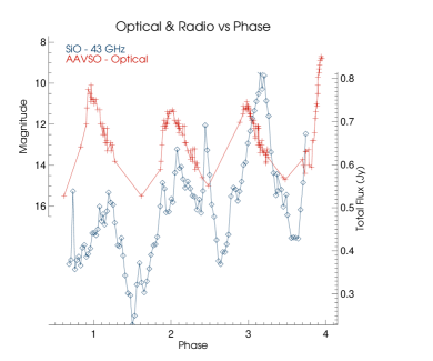
(a)

Figure 4: The visual magnitude (provided by AAVSO in red) and the radio flux density at 43 GHz in blue, plotted as a function of the stellar pulsation phase.

4 Shock Waves

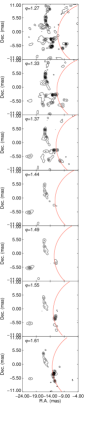
(a)

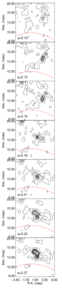
(b)

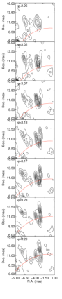
(c)

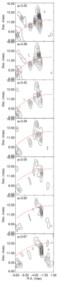
(d)

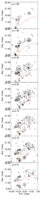
(e)

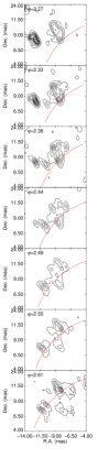
(f)

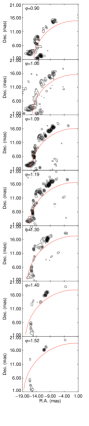
(g)

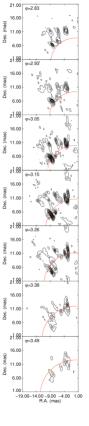
(h)

Figure 5: Each column is a collage of consecutive epochs, zoomed in to a feature of interest. In all the frames, the proposed shock is plotted as a red circle. The centre of the star is the centre of the circle. (a) Feature 3. A group of maser spots starts falling inwards; it appears that the encounter of these spots with the shock front results into a change of the direction of their motion. (b) Feature 5. The motion of this feature appears to be opposite to the global kinematic behaviour. However, as it meets the shock front, it changes direction following the overall outflow. (c) and (d) Feature 6. According to the proposed shock wave, this feature appears to be infalling. As it encounters the shock front, the feature changes its direction of motion. Then, as the shock propagates through the feature, it elongates it and eventually, breaks it down to into smaller spots. (e) and (f) Feature 4. This is the first split observed. The addition of the shock front reveals that the prominent double arc is not a split but a condensation of post-shock material that starts falling toward the star. The shock appears to be pushing the pre-shock material as it moves out. However, in column (f), which is an additional zoom into this infalling material, it appears that the new shock front splits it into two new but smaller arcs. (g) and (h) A comparison of the effects of the proposed shock. During the first cycle the shock appears to be pushing the material outwards. In contrast, in the last cycle observed, the shock seems to be penetrating the masering zone.

It is generally believed that in Miras a shock wave leaves the stellar surface once per stellar cycle, when the star is at its maximum (Bowen 1988; Humphreys et al. 2002). The effects of the passage of a shock through the extended atmosphere, where the SiO masers are located, could be visible in a number of ways. For example, a shock could split the ring to its pre- and post-shock components or make infalling material bounce back, forcing it to follow the shock’s motion. In order to study the effects of a shock wave in the masering zone and identify which component kinematics can be attributed to its passage, we created a second version of the movie, this time overlaying a shock wave.

For the radius of TX Cam we used the value from Cahn & Elitzur (1979) and also assumed a 20% change in the stellar radius due to pulsation (as motived by the data of Pettit & Nicholson (1933) and used in Reid & Menten (1997) and also observed by Wittkowski et al. (2007)). Additionally we adopted a shock velocity of 7 km s^-1, in line with the value of the initial velocity calculated for the inner shell boundary by Diamond & Kemball (2003) and Gonidakis et al. (2010). With these parameters we were able to calculate the radius of a uniform shock wave, leaving the stellar surface at maximum light. Once this information was also included in the frames, they were converted into a movie showing the propagation of the proposed shock. The movie is provided as online supplementary material and Fig. 7b shows its first frame.

Generally the shock appears to be intensifying the maser activity (Fig. 5h) or even creating maser spots as it passes through the masering zone; there are however occasions that this is not the case. Starting at $\phi\sim$ 0.64, the position of the shock coincides with most parts of the ring. The NE region however appears to be more curved than the spherical shock so that, as it propagates, it appears that it is pushing the material away from the star rather than penetrating this region. As a result of the curvature of this region, the shock reaches the east and north sides first, gradually gaining ground and at $\phi\sim$1.71 it passes over the last spot of the NE tip (Fig. 5g). Once overtaken, the spots fade away; however, on the eastern part, the material that the shock transits starts falling toward the star forming Feature 3.

The movie can also reveal whether the peculiar kinematics of the features described in § 3.1.3 are caused by the transition of a shock. Fig. 5a shows Feature 3, the first ricochet observed. As can be seen, as the spots infall they meet the shock front and, at $\phi$$\sim$1.44, they start changing the direction of their motion. The position of the shock at this phase coincides with the position where the change in the kinematics of the maser spots is observed. The addition of the shock front in the movie reveals also the true nature of the first split observed in Feature 4. It appears that the inner arc is not created by a split in the perimeter of the ring due to the shock but is actually infalling material, condensed in the post-shock region. The second split of this feature coincides perfectly with the passage of a shock through the ring, that splits it into two distinctive regions (Fig. 5e and 5f). Finally, both features 5 and 6 show an agreement between their kinematics and the position of the shock front. More specifically, Feature 5 seems to be infalling and then, as it meets the shock, it appears to become stationary and brightens as the shock propagates through its volume and then dissipates (Fig. 5b). The shock has a more dramatic influence in the structure of Feature 6; as it falls inward, it meets the shock that then drags it outward, breaking it up into smaller spots that eventually disappear (Fig. 5c and 5d).

5 Discussion

5.1 Variability

5.1.1 Maser Distribution

The most prominent overall property of the emission is its mostly circular distribution. The maser phenomenon is preferentially observed in directions along the line of sight, where the column density of SiO and velocity coherence are higher. In the extended atmospheres of AGB stars, where molecular species occupy shells around the star with radial acceleration due to shocks, this occurs in the tangent of the shell. This “tangential amplification pattern” is responsible for the ring-like structure of the masering areas. The cover factor, i.e the completeness of the ring, changes with the stellar pulsation and it appears that rings are formed preferentially near stellar maxima while, near minima, masers occupy a smaller percentage of their shell perimeters. Moreover, rings at the same phase do not exhibit the same characteristics. An inspection of the frames at phases 0.75, 1.74, 2.74 and 3.74 reveals that, although all correspond to the same pulsation phase of the ring, they can be significantly different. At $\phi$$\sim$0.75 the SE and NW arcs are missing, at $\phi$$\sim$1.74 the SE arc is faint but present, at $\phi$$\sim$2.74 a gap is located in the S sector, with the E-SE-S-SW part of the ring very faint while at $\phi$$\sim$3.74 the SW arc is missing with the SE-S-SW-W arc almost absent. These inconsistencies indicate that conditions can vary greatly around the star and local phenomena might be of particular importance. Moreover, the model of a spherical shell and a perfectly formed shock wave are clearly too simplistic to explain the variations we observe.

The variability in the distribution of the masers is not only observed in the degree of ring completeness but also in its radius relative to the star and its width. The study of the inner shell radius and the width revealed that the masering zone is neither located at a constant distance from the centre of the star nor does it have a constant width. It is a very dynamic region, revealing complex kinematics and its characteristics can change from cycle to cycle. The radius of the inner shell usually increases from minima to maxima and decreases from maxima to minima, causing the whole structure to alternately expand and contract. An exception to this behaviour is the first cycle observed, where the ring is continuously expanding. More importantly, the distance at which the ring forms is not correlated with the stellar phase; at the same phase during different cycles, rings can be located at different distances. The same appears to apply to the width of the ring; although it follows the stellar pulsation with a lag, it does not have the same characteristics at the same phases in different cycles. Both the inner radius and the width appear to be correlated with the SiO flux density and more intense rings are formed closer to the star and are wider. This also implies that wider rings are located closer to the star.

5.1.2 Flux Densities

The nature of the project allows us to study the flux variability of SiO masers not only in the short-term within a cycle, but also in the long-term, from one cycle to another. In line with Gonidakis et al. (2010), the sinusoidal pattern of the flux densiy of the emission reveals that it is correlated with the stellar phase (Hjalmarson & Olofsson 1979). On the other hand, the visual magnitude and radio flux density, appear to be uncorrelated in detail. Although all optical maxima appear to be equally strong, the 43 GHz flux densities at maxima appear to be increasing from cycle to cycle. The same applies to the minima, thus the contrast, i.e. the ratio of fluxes in consecutive maxima and minima, is not constant.

There is a clear, but not necessarily constant, lag between the visual magnitude and the 43 GHz flux density in all the cycles observed (Cho, Kaifu and Ukita 1988). A shock is believed to be created near the stellar surface once per stellar maximum (see $\S$5.2) and, if SiO masers are collisionally pumped, then the propagation of this shock through the masering zone can enhance maser activity; the observed lag could be attributed to the time needed for the shock to reach the masers. However, the strong correlation of the SiO flux densities with the 8 $\mu$m IR radiation (Bujarrabal, Planesas and del Romero 1988; Jewell et al. 1991), is a property that can support the radiative pumping scenario. Thus, the lag itself cannot be conclusive on the pumping mechanism of SiO masers.

5.2 Shock Waves

The idea of a shock wave in stars atmospheres was firstly suggested by Merrill (1921) in order to explain the big differences in the spectra of R Cyg. Gorbatskii (1961) produced the first theoretical model to show that emission lines can be associated with shock waves that heat the atmosphere while they propagate outwards through a low density region surrounding a long period star.

There are a number of features in the movie that are dominated by peculiar kinematics and we attempted to associate them with the existence of a shock wave permeating the extended atmosphere of TX Cam. As discussed in section 4, we overlayed in the movie a proposed shock wave, leaving the stellar surface once per cycle at the maximum. As can be seen in Fig. 5 the changes in the kinematics and the morphology of these features can be explained by the proposed shock wave, since they occur when the shock front encounters the maser spots.

The proposed shock appears to interact with the material in a number of ways. Predominantly the shock appears to permeate the masering zone, increasing the intensity of the maser spots (Fig. 5h). This could be the result of the increased rate of collisions due to the passage of the shock and evidence of the collisional pumping mechanism responsible for SiO masers. However, during the first cycle, the shock appears to be affecting only the kinematics of the ring, being the driving force that pushes the masering material to the furthest position observed throughout the movie (Fig. 5g). From our data we cannot conclude that the SiO masers are purely collisionally pumped; however, as in Cho, Kaifu and Ukita (1988), it appears that collisions play an important role in the pumping, especially around $\phi$$\sim$0.2.

5.3 Bipolarity?

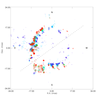
Figure 6: A figure showing contours maps of epochs BD46A, E, K and P (purple, blue, green and red respectively). The maps are overplotted to show the differences in expansion along the NE-SW and SE-NW axes. It is apparent that along the latter, the flow of material is faster.

The fit of a spherical shock wave revealed that the masering shell does not expand uniformly. A characteristic example is the expansion during the first cycle, where the masering ring appears to be more curved than the assumed perfectly circular shock. Could that be a hint of bipolar outflow around TX Cam? In order to examine this possibility we overlayed four different frames separated by five epochs to exaggerate the differences, as seen in Fig. 6. It is obvious that there are differences in the outflow, with spots in the NE-SW axis being stationary, while the SE-NW outflow appears to be the most intense. Another important observation is that the maser emission itself is manifestly different in these two directions. In the NE-SW direction there are clear gaps in the ring and emission is mainly diffuse. In contrast, the SE-NW spots are much brighter and compact. All the above constitute evidence of bipolar outflow around TX Cam.

It appears that a shock with velocity of 7 km s^-1(as modelled by Reid & Menten (1997)) is in good agreement with our data. According to our approach, the outer part of the ring is dominated by diffuse emission and was difficult to define robustly. However, we have calculated the radius of the inner boundary and the width of the ring so, their sum provides an estimate of the outer ring radius. The shape of the plot for the outer radius reveals a very important property of the masering shell: it follows the pulsation of the star with a small lag and it does not appear to be dependent on the overall kinematics of the inner shell, imposing an outer limit in the masering zone that is dependent only on the phase (Fig. 8). So, despite the lack of contraction during the first cycle, the average outer boundary of the ring is contracting; the constant expansion of the inner boundary is compensated by a thinner shell. This difference in the behaviour between the inner and outer radii of the ring, with the outer ring appearing unperturbed relative to its inner counterpart, might be an indication that the shocks at this distance are damped. This is in agreement with the result by Reid & Menten (1997) stating that any periodic shocks or disturbances near 2$R_{\star}$ probably propagate outward with velocities less than 5 km s^-1and are mostly damped.

5.4 Projection Effects

For the values of stellar radius and distance adopted here, one can calculate the distance of the masering zone from the surface of TX Cam. The unknown in this case is how much does TX Cam’s radius change from minimum to maximum. We calculated the distance of the ring from the surface of the star for several modes of pulsation, from 0-30%, and the surface in Fig. 2b shows the result of this approach. Mid-infrared interferometry of S Ori with the VLTI/MIDI (Very Large Telescope Interferometer/MID-infrared Interferometric instrument) at four epochs, revealed that the photospheric radius shows a significant phase-dependent size with amplitude of $\sim$20%, that is well correlated in phase with the visual lightcurve (Wittkowski et al. 2007). As discussed in $\S$5.2, for a 20% change in the stellar radius, the distance of the inner shell from the surface of TX Cam ranges from 5.35 to 12.34 mas. Additionally, during the same phase at different cycles, this distance can vary greatly; the inner shell in the first cycle at $\phi$$\sim$0.68 is located 1.67 times further than at $\phi$$\sim$3.68.

The previous result is somewhat peculiar, since it suggests that a significant change in the conditions on the extended atmosphere occurs in such a way, that the masering zone is systematically positioned closer to the star form one cycle to the next. Our results also suggest that the ring becomes brighter and thicker as we progress in cycles. These results are independent on the distance adopted in our study. The answer seems to be hidden in the velocity structure of the ring and the individual maser spots (an explanation of the aforementioned peculiarities will be given in the next paper of this series, where the velocity information will be included in our analysis). As previously observed by Yi et al. (2005) and Gonidakis et al. (2010), filaments exhibit a gradient along their axis, with values reaching the systemic velocity as we move along their axes toward the centre. Moreover, an examination of the radial velocities of the ring reveals that each cycle is very different kinematically along the line of sight. The ring during the first cycle is dominated by maser spots with velocities close to the systemic, but as we move in phase, spots appear systematically more blue- or red-shifted. This implies that projection effects are becoming more significant as we progress in phase. However, this also suggests that if projection is substantial, then a 3-dimensional study of the kinematics should be more appropriate in order to reveal the properties of the masering region.

5.5 Moving spots or change in conditions?

The maser spots appear to be moving, most of the time in an orderly manner, contributing to the global kinematic behaviour of expansion or contraction. But are we really witnessing the actual flow of material or is the emission tracing the changes in the physical conditions? As has been previously observed, the kinematics of the maser components follow ballistic motions, ruling out the latter scenario (Diamond & Kemball 2003). Additionally, there are components that exhibit kinematic properties consistent with motions along magnetic field lines (Kemball et al. 2011). There are also peculiarities that cannot be explained by the assumption that the flow is an illusion caused by the fact that the emission traces the advance of the physical conditions. The ricochets observed in the movie are difficult to explain only by the change in conditions, especially since the neighbouring features are exhibiting kinematics in line with the global behaviour.

There are features though where the effects of the change in physical conditions are apparent in their behaviour. Usually this is demonstrated with changes of the intensity within the masering spots. As the spots move following the global motion, the intensity peaks are redistributed within them in such a way that they resemble the changes in intensity in the lights of a christmas tree, thus the name ‘christmas tree effect’. This is observed in many of the filaments in the western part of the ring from $\phi$$\sim$1.56 to the end of the movie.

5.6 Comparison with Models

We will compare our observations with the latest and more complete model currently available, that of Gray et al. (2009). Results from TX Cam (Gonidakis et al. 2010) and R Cas (Assaf et al. 2011) have been previously compared with the same model. There are significant deviations between the model and our observational data. The model predicts that the diameter of the masering ring should be about twice the size of the stellar photosphere; however, there are variations around this value according to observations (Cotton et al. 2004; Wittkowski et al. 2007). If we assume a stellar photosphere of 4.33 mas for TX Cam (as derived from Cahn & Elitzur (1979) for the distance of 390 pc adopted here) it appears that the masering shell is located at distances greater than 2$R_{\star}$. The maximum distance of the inner shell is 16.24 mas (6.33 au or 3.74$R_{\star}$, the minimum is 10.03 mas (3.91 au or 2.32$R_{\star}$) while the weighted mean value over all our observations is only 13.27 mas (5.17 mas or 3.07$R_{\star}$).

An inconsistency between the model and our observations, is the phase at which the ring starts contracting. This structural change, according to Gray et al. (2009), happens between phases 0.1 and 0.25, when the ring starts decreasing in radius but increases in intensity. In our data, such a structural change should be demonstrated as a decrease in the inner shell boundary radius. However, contraction of the inner shell boundary is not observed at the phases predicted by Gray et al. (2009). In contradistinction, the behaviour of the outer boundary is in line with this result; the outer shell boundary radius starts decreasing at $\phi\sim$ 1.1, 2 and 3.1 respectively for each cycle. During the same phases ($\phi$$\sim$0.1 to 0.25), the model predicts an increase in the spectral output and this is observed in all the cycles covered by our data. The model also predicts a decrease in intensity between $\phi\sim$ 0.25-0.4 - this is also observed in our campaign. Another property that is not apparent in our data during these phases is the shift from a large number of spots of modest brightness to a smaller amount of spots, some of which appear very bright in the model.

There are a number of assumptions made in the creation of the model that could cause the disagreement with our data. The model assumes spherical symmetry for both the star and the shock, something that might not be true for TX Cam since, as described in § 5.3, there is strong evidence of bipolar outflow. As a matter of fact, asymmetries in Miras might be quite common and there is an increasing amount of observational evidence supporting this. CO(2-1) observations by Josselin et al. (2000) in $o$ Ceti revealed strong asymmetries in the gas distribution that could be explained by a bipolar outflow disrupting the spherical envelope. Thomson, Creech-Eakman & Akeson (2002) observed R Tri with the Palomar Testbed Interferometer and found that their data are not in agreement with a spherically symmetric model. Ragland et al. (2006) found asymmetric brightness distribution in 16 out of the 56 AGB stars they observed, using the Infrared Optical Telescope Array. Additionally, a restriction only to their well-resolved targets yielded asymmetry detections in 75% of the AGB and in 100% of the O-rich stars, allowing the authors to hypothesise that asymmetries might be detectable in all Miras.

The model assumes that the abundance of SiO is constant, independent of radius and phase, does not include SiO isotopologues and does not take into account the pulsation of the star. From our data, the distribution of the masers within the zone that could potentially host the effect, reveals that the conditions along the ring are not uniform. The many small gaps observed between individual maser spots could be caused by lower SiO density or lack of velocity coherence. On the other hand, the bigger and locally constant gaps can be attributed to the proposed bipolarity of TX Cam. The model can produce the former; the latter though, when simulated, is just the result of the random selection of the spots since individual spots in the model do not evolve, but the maser positions are rerandomised between each two phases. Moreover, our results for the outer bandary, which compares better with this model to its inner counterpart, suggests that the pulsation of the star influences the borders of the masering zone.

6 Conclusions

We presented the final version of the movie of the SiO masers in the extended atmosphere of the Mira Variable TX Cam. The movie covers three complete stellar pulsations from phase $\phi$=0.68 to 3.74. This paper is the first in a series presenting the results from this campaign and deals with the study of the structure and the global kinematic behaviour of the masering zone as well as the existence and contribution of shock waves to the observed properties. We conclude the following:
(i) The emission is confined to a narrow structure in accordance to previous results. This structure can change from a ring to an ellipsoid with significant asymmetries. The inner boundary of the ring reveals the global kinematic behaviour of the gas. Expansion and contraction are observed, although for the first cycle only expansion is observed.
(ii) The distribution of the masers is random along the perimeter of the ring. There are features that clearly deviate from the overall ordered kinematic behaviour and usually can be identified in the movie as splits or ricochets.
(iii) Most of the structural and physical properties follow the pulsation of the star, revealing a kinematic dependance with phase. Both the width of the ring and the outer boundary are correlated with the pulsation phase and the intensity appears to follow the stellar pulsation but with a lag.
(iv) There are a number of features with kinematics that can be attributed to the existence of shock waves. A shock with a velocity of 7 km s^-1can explain most of the observational peculiarities of these features. The morphology and evolution of the outer boundary suggests that at these distances shocks are damped.
(v) There is strong evidence that the outflow is bipolar. There is a clear difference in the expansion velocities along two perpendicular axes. In the SE-NW direction maser spots are brighter and are moving faster, while in the NE-SW direction the ring has clear gaps, with mainly diffuse emission that moves much slower.
(vi) Projection effects contribute to the overall appearance of the shell structure as revealed by their shifted radial velocities.
(vii) The agreement of our results with the current model seems to be dependent on our definition of the ring radius. The outer boundary seems to be following the behaviour predicted by the model of Gray et al. (2009) better than the inner shell.

Figure 8: This diagram shows the outer ring of the masering shell as calculated by the addition of the previously estimated quantities of the inner radius and the width.

We acknowledge with thanks data from the AAVSO International Database based on observations submitted to AAVSO by variable star observers worldwide.

Appendix A Total Intensity Frames

Fig. 9 is a collage of the total intensity frames. The phase of each frame is written at the top right of each contour plot and the date that the data were taken, above each frame. The lower contour value is 0.7 Jy/beam and the step between each contour is 2.22 Jy/beam until a maximum value of 45.5484 Jy/beam. For a better viewing result, the square root of the total intensity maps were used in the compilation of the movie, in order to reduce the dynamic range. However, the contour plots presented in this figure are the total intensity maps. The six features discussed in the text are also marked here. They are enclosed in rectangles at the epoch when they firstly appear or when a change in their kinematic behaviour is firstly clearly observed. The number next to the rectangle is the number of the feature as used in the text.

Figure 9: As explained in Appendix A

References

- Alcolea et al. (1999) Alcolea J., Pardo J. R., Bujarrabal V., Bachiller R., Barcia A., Colomer F., Gallego J. D., Gómez-González J., del Pino A., Planesas P., Rodríguez-Franco A., del Romero A., Tafalla M., de Vicente P., 1999, A&AS, 139, 461
- Assaf et al. (2011) Assaf K. A., Diamond P. J., Richards A. M. S. & Gray, M. D., 2011, MNRAS, 415, 1083
- Bowen (1988) Bowen G. H., 1988, ApJ, 329, 299
- Bujarrabal, Planesas and del Romero (1988) Bujarrabal V., Planesas P. and del Romero A., 1987, A&A, 175, 164
- Cahn & Elitzur (1979) Cahn J. H. and Elitzur M., 1979, ApJ, 231, 124
- Cho, Kaifu and Ukita (1988) Cho S-H., Kaifu N., Ukita N., 1996, AJ, 111, 1987
- Cotton et al. (2004) Cotton W. D. Mennesson B., Diamond P. J., Perrin G., Coudé du Foresto V., Chagnon G., van Langevelde H. J., Ridgway S., Waters R., Vlemmings W., Morel S., Traub W., Carleton N., and Lacasse M., 2004, A&A, 414, 275
- Deutsch & Merrill (1959) Deutsch A. J. & Merrill P. W., 1959, ApJ, 130, 570
- Diamond & Kemball (2003) Diamond P. J., Kemball A. J., 2003, ApJ, 599, 1372
- Diamond et al. (1994) Diamond P. J., Kemball A. J., Junor W., Zensus A., Benson J., Dhawan V., 1994, ApJ, 430, L61
- Elitzur (1992) Elitzur M.,1992, Astronomical Masers, Kluwer Academic Pblishers
- Elitzur (1980) Elitzur M., 1980, ApJ, 240, 553
- Gorbatskii (1961) Gorbatskii V. G., 1961, SvA, 5, 192
- Gonidakis et al. (2010) Gonidakis I., Diamond P. J., Kemball A. J., 2010, MNRAS, 406, 395
- Gray et al. (2009) Gray M. D., Wittkowski M., Scholz M., Humphreys E. L. M., Ohnaka K. & Boboltz D., 2009, MNRAS, 394, 51
- Gray et al. (1999) Gray M. D., Humphreys E. M. L., Yates J. A., 1999, MNRAS, 304, 906
- Greenhill et al. (1995) Greenhill L. J., Colomer F., Moran J. M., Backer D. C. Danchi, W. C. & Bester M., 1995, ApJ, 449, 365
- Habing (1996) Habing H. J.,1996, A&ARv, 7, 97H
- Habing & Olofsson (2004) Habing H. J. and Olofsson H., 2003, eds, Asymptotic Giant Branch Stars, (Springer, Heidelberg)
- Hjalmarson & Olofsson (1979) Hjalmarson Å., Olofsson H., 1979, ApJ, 234, L199
- Humphreys et al. (2002) Humphreys E. M. L., Gray M. D., Yates J. A., Field D., Bowen G. and Diamond P. J., 2002, A&A, 386, 256
- Jewell et al. (1991) Jewell P. R., Snyder L. E., Walmsley C. M., Wilson T. L., GensheimerP. D., 1991, A&A, 242, 211
- Josselin et al. (2000) Josselin E., Mauron N., Planesas P., Bachiller R., 2000, A&A, 362, 255
- Kemball et al. (2011) Kemball A. J., Diamond P. J., Richter L., Gonidakis I. & Xue R., 2011, ApJ, 743, 69
- Kemball and Diamond (1997) Kemball A. J., Diamond P. J., 1997, ApJ, 481, L111
- Kemball, Diamond and Cotton (1995) Kemball A. J., Diamond P. J., Cotton, W. D., 1995, A&AS, 110, 383K
- Kholopov et al. (1985) Kholopov P. N., Samus N. N., Frolov M. S., Goranskij V. P., Gorynya N. A., Kireeva N. N., Kukarkina N. P., Kurochin N. E., Medvedeva G. I., Perova N. B., Shugarov S. Y., 1985, General Catalogue of Variable Stars, Moscow Publishing House, Moscow
- Olivier, Whitelock and Marang (2001) Olivier E. A., Whitelock P. and Marang F., 2001, MNRAS, 226, 490
- Olofsson (2001) Olofsson H., 2001, ASPC, 235, 355O
- Merrill (1921) Merrill P.W., 1921, ApJ, 53, 185
- Miyoshi et al. (1994) Miyoshi M., Matsumoto K., Kameno S., Takaba H., & Iwata T., 1994, Nature, 371, 395
- Pardo et al. (2004) Pardo J. R., Alcolea J., Bujarrabal V., Colomer F., del Romero A. and de Vicente P., 2004, A&A, 424, 145
- Pettit & Nicholson (1933) Pettit E. & Nicholson, S. B. 1933, ApJ, 78, 320
- Poggendorff (1863) Poggendorff, J. C. 1863, Bibliographisch-Literaturisches Handw rterbuch zur Geschichte der Exacten Wissenschaften, Verlag Johann Ambrosius Barth, Leipzig, 1, 712
- Ragland et al. (2006) Ragland S., Traub W. A., Berger J.-P., Danchi W. C., Monnier J. D., Willson L. A., Carleton N. P., Lacasse M. G., Millan-Gabet R., Pedretti E., Schloerb F. P., Cotton W. D., Townes C. H., Brewer M., Haguenauer P., Kern P., Labeye P., Malbet F., Malin D., Pearlman M., Perraut K., Souccar K. and Wallace G., 2006, ApJ, 652, 650
- Reid & Goldston (2002) Reid M. J. & Goldston J. E., 2002, ApJ, 568, 931
- Reid & Menten (1997) Reid M. J. & Menten K. M., 1997, ApJ, 476, 346
- Thomson, Creech-Eakman & Akeson (2002) Thompson R. R., Creech-Eakman M. J., AkesonR. L., 2002, ApJ, 570, 373
- Wittkowski et al. (2007) Wittkowski M., Boboltz D.A., Ohnaka K., Driebe T., and Scholz M., 2007, A&A, 470, 191
- Wolf (1877) Wolf, R. 1877, Geschichte der Astronomie, Verlag R. Oldenbourg, Munchen, p. 116
- Yi et al. (2005) Yi J., Booth R. S., Conway J. E. & Diamond P. J., 2005, A&A, 432,531