Interpretation of the measurements
of total, elastic and diffractive cross sections at LHC

Abstract

Recently at LHC one has obtained measurements of the total, elastic and diffractive cross sections in $pp$ collisions at very high energy. The total cross section is in good agreement with predictions based on a leading behavior $\sigma_{\rm tot}(s)\propto(\ln s/s_{0})^{2}$, on the other hand the elastic cross section is lower than most expectations and the diffractive cross section is higher. It is remarkable that the ratio $(\sigma_{\rm el}+\sigma_{\rm diff})/\sigma_{\rm tot}$ calculated combining the results of the TOTEM and ALICE detectors is $0.495^{+0.05}_{-0.06}$, very close to the maximum theoretically allowed value of 1/2 known as the Miettinen Pumplin bound. In this work we discuss these results using the frameworks of single and multi–channel eikonal models, and outline the main difficulties for a consistent interpretation of the data.

I Introduction

The data obtained at the CERN LHC has allowed to significantly extend the energy range for the study of proton–proton collisions. The main focus of the LHC program is the study of rare processes and the search for new physics phenomena, but they also allow to measure “average properties” of the $pp$ interactions, such as the total and elastic cross section, multiplicity distributions and inclusive spectra in different kinematical variables (energy, rapidity, pseudo–rapidity or transverse momentum). These studies have an intrinsic interest because they test our understanding of the strong interactions, and at the same time they are important for the interpretation of the observations of ultra high energy cosmic rays (UHECR). The spectrum of these particles extends to $E_{\rm lab}\simeq 10^{20}$ eV, that corresponds to a nucleon–nucleon c.m. energy $\sqrt{s}\simeq 433$ TeV, and the modeling of their atmospheric showers requires an extrapolation of the LHC results that should be based on a reasonably robust theoretical understanding of the underlying hadronic physics.

The TOTEM detector Antchev:2011vs ; totem-a ; Antchev:2011zz ; totem-b ; totem-c ; totem-d has obtained measurements of the $pp$ total and elastic cross sections at $\sqrt{s}=7$ and 8 TeV. These results extend considerably the energy range where these cross sections are known, and constitute a very important constraint for the extrapolations of $\sigma_{\rm tot}^{pp}$ and $\sigma_{\rm el}^{pp}$ up to the UHECR energy range. Measurements of the inelastic cross sections at $\sqrt{s}=7$ TeV have also been obtained by the ALICE, ATLAS and CMS detectors alice-sigma ; atlas-sigma ; cms-sigma . It should be noted that the interaction length of high energy protons and nuclei in air is determined by the combination of the total and elastic cross sections, so that an understanding of the energy dependence of both quantities is needed.

The ALICE collaboration has also published measurements of the inelastic diffraction cross section at $\sqrt{s}=0.9$, 2.3 and 7 TeV in the form of the ratios $\sigma_{SD}/\sigma_{\rm inel}$ and $\sigma_{DD}/\sigma_{\rm inel}$, where SD (DD) stands for single (double) diffraction. In inelastic diffraction one (or both) of the colliding protons is excited into a state with the same internal quantum numbers of the initial particle. Summing over single and double diffraction, the diffractive processes account for approximately one third of the inelastic cross section. It is interesting to note that the sum of the elastic and diffraction cross sections is consistent with the saturation of the theoretical bound established by Miettinen and Pumplin Miettinen:1978jb , according to which $\sigma_{\rm diff}+\sigma_{\rm el}\leq\sigma_{\rm tot}/2$. It is also intriguing that at LHC energies the elastic and diffractive cross section are approximately equal.

A good knowledge of the size of the diffraction cross section is phenomenologically important for the modeling of UHECR showers because the properties of the final state in diffractive events are significantly different than for the rest of inelastic interactions. From the theoretical point of view a good description of diffraction is an important test.

The observations of ALICE, ATLAS, CMS and LHCb have also provided many observations of the properties of particle production in inclusive (or “minimum bias”) $pp$ interactions. These observations show that the average charged multiplicity, and the average density of particles per unit of pseudorapidity in the central region increases with energy rapidly (faster than most predictions), and have large fluctuations (broader than most predictions). These measurements are confined to the central region of phase space, and do not include particles emitted at very small angles with respect to the beam directions. Very valuable observations of the energy spectra of photons and neutral pions emitted at very small angles have been obtained by the LHCf detector Adriani:2011nf .

In our view, all properties of high energy hadronic interactions: total, elastic and diffractive cross sections, average multiplicities, inclusive energy spectra are associated to the same fundamental underlying dynamics, and require a comprehensive and consistent description. The fundamental idea underlying such a comprehensive description of the properties of inclusive hadronic interactions, is that hadrons are composite objects formed by an ensemble of quarks and gluons, and that in a single $pp$ (or more in general hadron–hadron) collision there are several parton–parton interactions. With increasing energy a larger number of parton–parton collisions becomes possible, and this drives at the same time the growth of the hadron–hadron cross sections and the growth of the particles multiplicity in the final state (with a corresponding softening of the inclusive energy spectra). A comprehensive model should therefore be able to relate the energy dependence of the parton–parton and hadron–hadron cross sections, and then also connect the underlying parton structure of the collision to the observable final state particles. The LHC data are of course essential for the development of such a comprehensive model for hadronic interactions at high energy.

The LHC results on the total, elastic and diffractive cross sections have been the object of several theoretical studies, see for example Ryskin:2012az ; Gotsman:2012rq ; Gotsman:2012rm ; Grau:2012wy ; Kopeliovich:2012yy ; Fagundes:2012rr .

This work is organized as follows: in the next section we list and briefly discuss the measurements of the total, elastic and diffractive cross sections at LHC. In section 3 we introduce the definitions of the opacity and eikonal functions $\Gamma(b,s)$ and $\chi(b,s)$, and estimate these functions from the data on the elastic cross sections obtained by TOTEM at $\sqrt{s}=7$ TeV, and compare with data at lower energy. In section 4 and 5 we try to interpret these results in the frameworks of single and multi–channel eikonal models. The last section contains some discussion.

II Cross section measurements at LHC

Recently the TOTEM collaboration has measured Antchev:2011vs ; totem-a ; Antchev:2011zz ; totem-b ; totem-c ; totem-d the total, elastic and inelastic cross sections in $pp$ collisions at $\sqrt{s}=7$ and 8 TeV. The cross sections at $\sqrt{s}=7$ TeV have been obtained using two different methods. The first one Antchev:2011vs ; totem-a ; Antchev:2011zz makes use of the luminosity measurements of the CMS detector, and is based on the measurement of elastic scattering, with the total cross section obtained via the optical theorem; the second one totem-b ; totem-c ; totem-d is independent from a luminosity measurements and relies on measurements of elastic an inelastic events (and again the optical theorem). At $\sqrt{s}=8$ TeV the cross sections measurements totem-d have been presented only for the luminosity independent method.

At $\sqrt{s}=7$ TeV, the TOTEM collaboration has measured the differential elastic scattering cross section in the range $0.005\leq|t|\leq 0.47$ GeV², with $t=(p-p^{\prime})^{2}$ the squared momentum transfer Antchev:2011zz ; Antchev:2011vs ; totem-a . Extrapolating the data to $t=0$, and using the CMS luminosity measurement, the collaboration obtains Antchev:2011vs a total elastic cross section $\sigma_{\rm el}=24.8\pm 1.2$ (or $25.4\pm 1.1$ in totem-a ). The data on the elastic cross section are shown in fig. 1. For a comparison to lower energy data, fig. 2 shows the data Nagy:1978iw ; Ambrosio:1982zj ; Breakstone:1984te on elastic scattering obtained at ISR for $\sqrt{s}=53$ GeV, where the data extends to a very broad range in $t$.

The differential elastic cross section can be written in terms of the scattering amplitude $F_{\rm el}(t,s)$ as:

$$\frac{d\sigma_{\rm el}}{dt}(t,s)=\pi\;\left|F_{\rm el}(t,s)\right|^{2}\;.$$ (1)

The optical theorem gives a relation between the total cross section and the imaginary part of the forward elastic scattering amplitude:

$$\sigma_{\rm tot}(s)=4\,\pi\;\Im[F_{\rm el}(0,s)]=\frac{4\,\sqrt{\pi}}{\sqrt{1+\rho^{2}}}\;\left[\left.\frac{d\sigma_{\rm el}}{dt}\right|_{t=0}\right]^{1/2}$$ (2)

where we have used the notation $F_{\rm el}(0,s)=\Im\left[F_{\rm el}(0,s)\right]\;(i+\rho)$ so that $\rho$ is the ratio of the real to imaginary part of the forward elastic scattering amplitude.

Extrapolating the elastic cross section measurements to $t=0$ and using the prediction $\rho\simeq 0.145\pm 0.007$ at $\sqrt{s}=7$ TeV from the COMPETE group Cudell:2002xe , the TOTEM collaboration arrives to the result Antchev:2011vs $\sigma_{\rm tot}=98.3\pm 2.8$ mb (or $\sigma_{\rm tot}=98.6\pm 2.2$ mb in totem-a ). By subtraction one obtains $\sigma_{\rm inel}=73.5\pm 1.6$ mb (or $73.2\pm 1.3$ mb).

The luminosity independent method relies on the measurement of integrated number of elastic and inelastic events ($N_{\rm el}$ and $N_{\rm inel}$) combined with the measurement of the quantity $\left.dN_{\rm el}/dt\right|_{t=0}$. Using this method at $\sqrt{s}=7$ TeV totem-b ; totem-c the TOTEM collaboration obtains at 7 TeV: $\sigma_{\rm tot}=98.0\pm 2.5$, $\sigma_{\rm el}=25.1\pm 1.1$ and $\sigma_{\rm inel}=72.9\pm 1.5$, in good agreement with the results obtained by the previous method. The results can be combined with the luminosity measurement of CMS to estimate $\rho=0.145\pm 0.091$ in excellent agreement with the COMPETE prediction.

At $\sqrt{s}=8$ TeV totem-d the luminosity independent method gives $\sigma_{\rm tot}=101.7\pm 2.9$, $\sigma_{\rm el}=27.1\pm 1.4$ and $\sigma_{\rm inel}=74.7\pm 1.7$.

For an understanding of the dynamics that determines the total and elastic cross section it is important to also measure the inelastic diffraction cross section. The ALICE collaboration alice-sigma has recently published measurements of this component of the $pp$ cross section at LHC. The rate of diffractive events is estimated from a study of gaps in the pseudorapidity distributions of charged particles. For a diffractive mass $M_{X}^{2}<200$ GeV² the fraction of single diffraction processes in inelastic collisions at $\sqrt{s}=0.9$, 2.36 and 7 TeV is estimated as: $\sigma_{\rm SD}/\sigma_{\rm inel}=0.21\pm 0.03$, $0.20^{+0.07}_{-0.08}$, and $0.20^{+0.04}_{-0.07}$. For double diffraction processes (with a pseudorapidity gap $\Delta\eta>3$), for the same c.m. energies, ALICE finds: $\sigma_{\rm DD}/\sigma_{\rm inel}=0.11\pm 0.03$, $0.12\pm 0.05$, and $0.12^{+0.05}_{-0.04}$.

Support for a large cross section for inelastic diffraction also comes from a comparison of the measurements of the inelastic cross sections at $\sqrt{s}=7$ TeV obtained by the ATLAS atlas-sigma and CMS cms-sigma collaborations, with the TOTEM results. The measurements of $\sigma_{\rm inel}$ of ATLAS and CMS are based on a direct method, and require a model dependent correction to take into account the fact that an important fraction of the diffractive events is not observable. On the other hand the measurement of the inelastic cross section in TOTEM that is obtained as the difference between $\sigma_{\rm tot}$ and $\sigma_{\rm el}$ is independent from the size of the diffractive cross section. To reconcile the estimates of $\sigma_{\rm inel}$ of all experiments it is necessary to include a large $\sigma_{\rm diff}$.

Combining the results of ALICE and TOTEM one can estimate at $\sqrt{s}=7$ TeV the ratios

$$\frac{\sigma_{\rm diff}}{\sigma_{\rm tot}}\simeq 0.24~{}^{+0.05}_{-0.06}$$ (3)

and

$$\frac{\sigma_{\rm el}+\sigma_{\rm diff}}{\sigma_{\rm tot}}=0.495^{+0.05}_{-0.06}~{}.$$ (4)

Miettinen and Pumplin Miettinen:1978jb have argued that the sum of the diffractive and elastic cross section must respect the bound:

$$\frac{\sigma_{\rm el}+\sigma_{\rm diff}}{\sigma_{\rm tot}}\leq\frac{1}{2}\;.$$ (5)

A derivation of the bound is also given below in section V. The combined measurements of TOTEM and ALICE indicate that the Miettinen–Pumplin bound is close to saturation at LHC energies. This is a remarkable result that had not been predicted, and is in need of a convincing dynamical explanation.

It is also interesting that the elastic and diffractive cross sections at $\sqrt{s}=7$ TeV are consistent with being equal:

$$\frac{\sigma_{\rm diff}}{\sigma_{\rm el}}=0.952^{+0.20}_{-0.24}~{}.$$ (6)

This is likely to be only an accident, but it is possible to speculate whether, with increasing $\sqrt{s}$, the ratio $\sigma_{\rm diff}/\sigma_{\rm el}$ will stabilize to a constant value or decrease.

III Opacity and eikonal functions

In order to construct models of the total and elastic cross sections based on the partonic structure of the colliding hadrons it is useful to study the collisions in impact parameter space. This allows the definition and construction of quantities (such as the the opacity and eikonal functions) that can then be more directly interpreted in terms of elementary parton interactions.

The elastic scattering amplitude $F_{\rm el}(t,s)$ can be written as a two–dimensional integral over impact parameter:

$$F_{\rm el}(t,s)=i\;\int\frac{d^{2}b}{2\,\pi}~{}e^{i\vec{q}.\vec{b}}~{}\Gamma(b,s)\;.$$ (7)

In this equation the 2–dimensional vector $\vec{q}$ gives the spatial components of the transverse momentum. At high energy and small $|t|$, to a very good approximation one has: $|\vec{q}|^{2}=-t$. The quantity $\Gamma(b,s)$ is the opacity function that can be written in terms of the eikonal function $\chi(b,s)$:

$$\Gamma(b,s)=1-e^{-\chi(b,s)}\;.$$ (8)

Substituting the expression (7) for the amplitude into (1) and integrating over all $t$ (over $d^{2}q$) one obtains:

$$\sigma_{\rm el}(s)=\int d^{2}b~{}\left|\Gamma(b,s)\right|^{2}~{}.$$ (9)

From the optical theorem one has:

$$\sigma_{\rm tot}(s)=2\;\int d^{2}b~{}\Re\left[\Gamma(b,s)\right]~{}.$$ (10)

Combining equations (9) and (10) one also obtains:

$$\sigma_{\rm inel}(s)=\int d^{2}b~{}\left\{1-\left|1-\Gamma(b,s)\right|^{2}\right\}~{}.$$ (11)

In the following we will make the approximation to neglect the real part of the elastic scattering amplitude. This is incorrect because in this situation the amplitude has not the required analiticity properties. The approximation is reasonable, since $\rho(s)$, the ratio of the real to imaginary part of the amplitude at $t=0$ is small. The assumption of a purely imaginary amplitude implies that the opacity and eikonal functions are real, and a physical interpretation of these objects in terms of parton–parton interactions becomes easier.

The width of $\Gamma(b,s)$, or more precisely the average value $\langle b^{2}(s)\rangle$, is directly proportional to the slope $B_{\rm el}(s)$ of the differential cross section at $t=0$ ($d\sigma_{\rm el}/dt\propto e^{B_{\rm el}\,t}$). From the definition:

$$B_{\rm el}(s)=\left[\left(\frac{d\sigma_{\rm el}}{dt}~{}\right)^{-1}\frac{d}{dt}\left(\frac{d\sigma_{\rm el}}{dt}\right)\right]_{t=0}~{},$$ (12)

and using equations (1) and (7) one can derive the expression:

$$B_{\rm el}(s)=\left\{\int d^{2}b~{}\frac{b^{2}}{2}~{}\Gamma(b,s)\right\}\times\left\{\int d^{2}b~{}\Gamma(b,s)\right\}^{-1}=\frac{\langle b^{2}\rangle}{2}\;,$$ (13)

The elastic scattering cross section $d\sigma_{\rm el}/dt$ is well described (see fig. 1 and 2) by a simple exponential of constant slope for $|t|$ not too large. Using the approximation that the form $d\sigma_{\rm el}/dt\propto e^{B_{\rm el}\,t}$ is valid for all $t$ one can write the elastic cross section as:

$$\sigma_{\rm el}(s)\simeq\pi~{}\frac{\left|F_{\rm el}(0,s)\right|^{2}}{B_{\rm el}(s)}=\frac{\sigma_{\rm tot}^{2}\;(1+\rho^{2})}{16\,\pi\,B_{\rm el}}~{},$$ (14)

(in the second equality we have used the optical theorem). This equation relates $\sigma_{\rm tot}$, $\sigma_{\rm el}$ and the slope $B_{\rm el}$ (with a smaller role played by $\rho$).

The opacity function $\Gamma(b,s)$ can be obtained from the elastic scattering amplitude inverting equation (7):

$$\Gamma(b,s)=-i\;\int_{0}^{\infty}d|t|~{}J_{0}(b\,\sqrt{|t|})~{}F_{\rm el}(t,s)$$ (15)

In general it is not possible to use the above equation to evaluate numerically $\Gamma(b,s)$ from a measurement of the differential elastic scattering cross section because one lacks information about the phase of amplitude. However, it is known that the elastic scattering amplitude is in first approximation purely imaginary, and also that at $t=0$ this imaginary part is positive, since it is related by the optical theorem to the total cross section. If one makes the approximation to neglect the real part of the amplitude and in addition one assumes that the derivative (with respect to $t$) of the amplitude has no discontinuities, the phase ambiguity is resolved. The (purely real) opacity function can then be obtained with the numerical integration:

$$\Gamma(b,s)=\frac{1}{\sqrt{\pi}}\;\int_{0}^{\infty}d|t|~{}J_{0}(b\,\sqrt{|t|})~{}\sqrt{\frac{d\sigma_{\rm el}}{dt}}\;{\rm sign}(t,s)\;.$$ (16)

(where the sign is $+1$ at $t=0$, and changes at each zero of the cross section).

We have used equation (16) to estimate numerically the profile and eikonal function from the experimental data. Using for $d\sigma_{\rm el}/dt$ the fit to the data shown in fig. 1 and 2 one obtains the profile functions $\Gamma(b,s)$ shown in fig. 3. The data covers only a finite range of $t$, but the extrapolation to large $-t$ introduces a negligible error when $b$ is not too large. With increasing $s$ the opacity function becomes larger and broader, remaining (as expected) always in the range $0\leq\Gamma(b,s)\leq 1$.

The corresponding eikonal functions can be calculated from the definition (8) and are shown in fig. 4. Without loss of generality the function $\chi(b,s)$ can be written as the product:

$$\chi(b,s)=\frac{1}{2}\;A_{\chi}(b,s)\;\sigma_{\rm eik}(s)$$ (17)

where the quantity $\sigma_{\rm eik}(s)$ (with the dimensions of a cross section) can be obtained performing the integration:

$$\sigma_{\rm eik}(s)=2\;\int d^{2}b~{}\chi(b,s)\;,$$ (18)

and the function $A_{\chi}(b,s)$ (with the dimensions of the inverse of a cross section) is normalized to unity:

$$\int d^{2}b~{}A_{\chi}(b,s)=1\;.$$ (19)

For the opacity functions shown in figures 3 and 4 one obtains $\sigma_{\rm eik}(s)\simeq 55\pm 1$ mb at $\sqrt{s}=53$ GeV and $\sigma_{\rm eik}(s)\simeq 156\pm 14$ mb at $\sqrt{s}=7$ TeV. The shapes of the eikonal functions are shown in fig. 4. With increasing $\sqrt{s}$ the function $A_{\chi}(b,s)$ becomes broader: At $\sqrt{s}=53$ GeV one has $\sqrt{\langle b^{2}\rangle}\simeq 0.93\pm 0.01$ fm, at 7 TeV $\sqrt{\langle b^{2}\rangle}\simeq 1.09\pm 0.02$ fm.

To have an analytic approximation for the $b$ dependence of the eikonal function we have used the form:

$$A_{\chi}(b,s)\simeq A_{*}[b,r_{0}]=\frac{1}{96\,\pi\;r_{0}^{2}}\;\left[\frac{b}{r_{0}}\right]^{3}\;K_{3}\left(\frac{b}{r_{0}}\right)$$ (20)

that depends on the single parameter $r_{0}$, that must be considered as a function of $s$, and is proportional to the width of the distribution:

$$\left\langle b^{2}(s)\right\rangle=16\,r_{0}^{2}(s)~{}.$$ (21)

The expression (20) corresponds to the geometrical overlap of two normalized, spherical exponential distributions ($\rho(r)\propto e^{-r/r_{0}}$) separated by the transverse distance $b$:

$$A_{*}(b)=\int d^{3}r_{1}\;\int d^{3}r_{2}~{}\rho(r_{1})\;\rho(r_{2})~{}\delta^{(2)}(\vec{r}_{\perp 1}-\vec{r}_{\perp 2}+\vec{b})~{}.$$ (22)

This can be verified noting that the Fourier transform of an exponential distribution is $(1+q^{2}\,r_{0}^{2})^{-2}$, and the Fourier transform of expression (20) is:

$$\hat{A}_{*}(q)=(1+q^{2}\,r_{0}^{2})^{-4}\;.$$ (23)

The proton electromagnetic form factor has also the form $(1+R_{p}^{2}\,q^{2})^{-2}$ (with $R_{p}\simeq 0.234$ fm), and on this basis the functional form (20), (with the parameter $r_{0}$ fixed at the value $r_{0}=R_{p}$) was proposed by Durand and Pi Durand:1988cr as the $b$ dependence of the eikonal function, and then used in several other works, sometimes leaving $r_{0}$ as a free parameter.

In fig. 4 the dashed lines show the function $A_{*}(b,r_{0})$ with the parameter $r_{0}$ chosen to reproduce the width of the eikonal function $\chi(b,s)$ obtained numerically. The functional form (20) is an excellent description of the shape of the eikonal at $\sqrt{s}=53$ GeV and remains a reasonably good description at $\sqrt{s}=7$ TeV, where some small deviations become apparent.

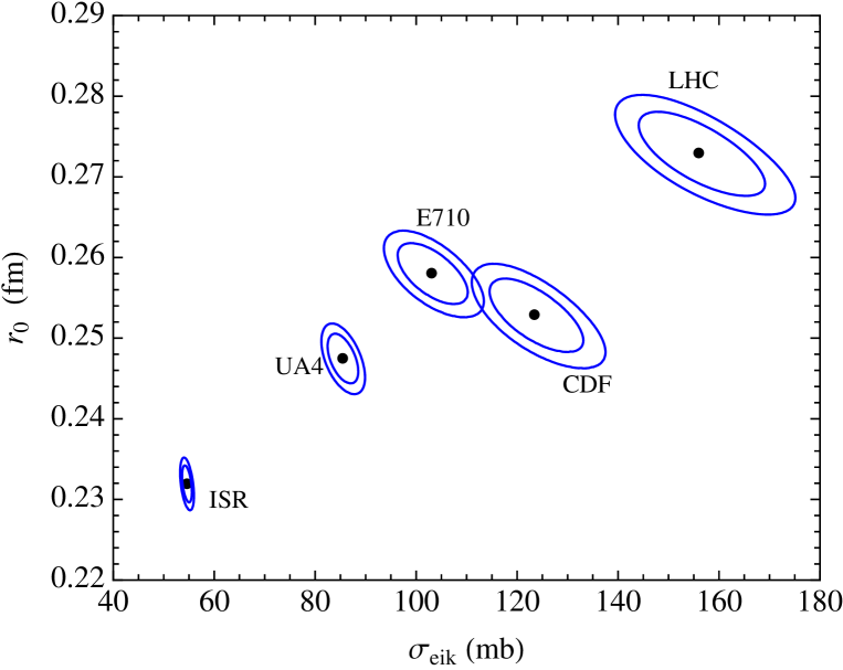
Figure 5: Regions in the plane $\{\sigma_{\rm eik},r_{0}\}$ that corresponds to the measurements of $\sigma_{\rm tot}$ and $B_{\rm el}$ for $pp$ and $\overline{p}p$ collisions at different c.m. energies. The different regions are for $pp$ collisions at $\sqrt{s}=53$ GeV (ISR), and $\sqrt{s}=7$ TeV (LHC); and $\overline{p}p$ collisions at $\sqrt{s}=546$ GeV (UA4), and $\sqrt{s}=1.8$ TeV (CDF) and (E710).

Allowed regions (at 68% and 90% C.L.) for the parameters $\sigma_{\rm eik}$ and $r_{0}(s)$ that describe the experimental data are shown in fig. 5. In the figure we also show the results for $\overline{p}p$ scattering at $\sqrt{s}=0.546$ and 1.8 TeV. At $\sqrt{s}=1.8$ TeV the measurements of CDF Abe:1993xx ; Abe:1993xy and E811 Avila:1998ej are in poor agreement with each other and are treated independently.

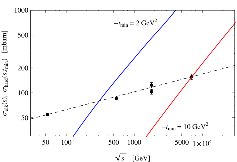
Figure 6: The points are estimates of the quantity $\sigma_{\rm eik}(s)$ shown in fig. 5, plotted as a function of $\sqrt{s}$. The thick lines are calculation of the cross section for hard parton–parton scattering in $pp$ collisions in the kinematical regions $-t\geq 2$ GeV² and $-t\geq 10$ GeV². The calculation using LO cross parton cross sections and the PDF’s of MRSTW Martin:2009iq . The dashed line, drawn to guide the eye corresponds to $23~{}mb\times(s/{\rm GeV}^{2})^{0.11}$.

The energy dependences of the quantities $\sigma_{\rm eik}(s)$ and $\sqrt{\langle b^{2}(s)\rangle_{\chi}}$ are shown in fig. 6 and 7. The quantity $\sigma_{\rm eik}(s)$ grows approximately as a power law ($\sigma_{\rm eik}(s)\propto s^{0.11}$), while the width of the eikonal function grows approximately logarithmically with $s$.

Evidence for the energy dependence of the width of the eikonal function can also be seen from a study of the relation between the total cross section $\sigma_{\rm tot}$ and the slope $B_{\rm el}$, or equivalently between $\sigma_{\rm tot}$ and the ratio $\sigma_{\rm el}/\sigma_{\rm tot}$. These relations are not independent because the three quantities $\sigma_{\rm tot}$, $\sigma_{\rm el}$ and $B_{\rm el}$, in the approximation of a real elastic scattering amplitude (or $\rho^{2}\ll 1$), are related by the optical theorem (14).

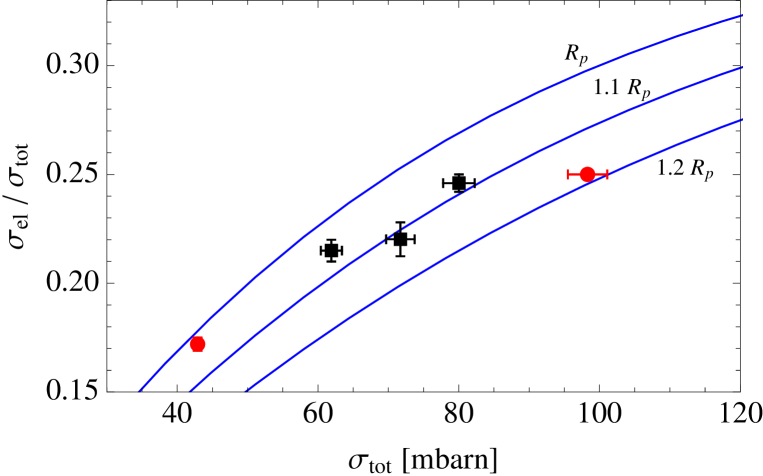
Figure 9: Plot of the relation $\sigma_{\rm el}/\sigma_{\rm tot}$ versus $\sigma_{\rm tot}$. The (red) disks are measurements for $pp$ scattering at ISR ($\sqrt{s}=53$ GeV) and LHC ($\sqrt{s}=7$ TeV); the (black) squares are measurements for $\overline{p}p$ scattering at CERN ($\sqrt{s}=546$ GeV) and Fermilab ($\sqrt{s}=1.8$ TeV). The lines describe the relation when the eikonal function has the $b$ dependence of equation (20) with the parameter $r_{0}$ given by $1$, 1.1 and 1.2 times $R_{p}$ (with $R_{p}$ obtained from the electromagnetic form factor).

If one assumes that all the energy dependence is contained in the eikonal cross section, the darkening and broadening of the the opacity function with increasing $\sigma_{\rm eik}$ are not independent. Accordingly, for any value of the total cross section (that is proportional to the area under $\Gamma(b,s)$) one can compute the slope $B_{\rm el}$ (that measures the width of $\Gamma(b,s)$) or the ratio $\sigma_{\rm el}/\sigma_{\rm tot}\propto\sigma_{\rm tot}/B_{\rm el}$. The data, as illustrated in fig. 8 and fig. 9, indicate that the increase in the slope is faster, and the increase in the ratio $\sigma_{\rm el}/\sigma_{\rm tot}$ is slower than a prediction based on a constant width for the eikonal function, indicating that a broadening for increasing $\sqrt{s}$ is necessary.

IV Single channel eikonal model

In a broad range of models Gaisser:1984pg ; Pancheri:1985ix ; Durand:1988cr , the eikonal function $\chi(b,s)$ is interpreted as proportional to $n(b,s)$, the average number of “elementary interactions” in a collision at impact parameter $b$ and c.m. energy $\sqrt{s}$:

$$n(b,s)=2\,\chi(b,s)\;.$$ (24)

This interpretation arises from the fact that (using the approximation of a real eikonal function) one can rewrite the expression for the inelastic cross section (11) in the form:

$$\sigma_{\rm inel}(s)=\int d^{2}b~{}\left[1-e^{-2\chi(b,s)}\right]$$ (25)

The structure of this equation suggests that the quantity $1-e^{-2\,\chi(b,s)}$ has the physical meaning of the absorption probability in collisions at impact parameter $b$. If the absorption probability is understood as the probability of having at least one elementary interaction in the collision, and in addition one assumes that the fluctuations in the number of elementary interactions in the collisions at fixed $b$ and $s$ have a Poissonian distribution, one can interpret the quantity $2\,\chi(b,s)$ as the average number of interactions, arriving to equation (24).

Using the factorization of equation (17), one can see that from the assumption of equation (24) one can conclude that both $\sigma_{\rm eik}(s)$ and $A_{\chi}(b,s)$ have simple and direct physical interpretations. The quantity $\sigma_{\rm eik}(s)$ corresponds to the parton–parton cross section at c.m. energy $\sqrt{s}$, and $A_{\chi}(b,s)$ is interpreted as the overlap of the spatial distributions of the interacting partons.

A fundamental problem for all models that attempt to describe the total cross sections in terms of parton constituents in the colliding hadrons is to compute in a consistent way a cross section that accounts for all elementary parton scatterings. In QCD a parton–parton cross section is well defined and calculable only for a momentum transfer sufficiently large. For $Q^{2}\to 0$ the perturbation theory expressions for the cross sections diverge, but perturbation theory is not applicable, and in fact also the identification of the partons in the colliding hadrons is uncertain.

Several ideas have been put forward to compute a finite cross section that accounts for all soft parton interactions, but the problem remains open. In this work we do not address this question but only try to estimate a lower limit on this quantity. The parton cross section can be decomposed into hard and soft components:

$$\sigma_{\rm parton}(s)=\sigma_{\rm hard}(s,|t_{\rm min}|)+\sigma_{\rm soft}(s,|t_{\rm min}|)~{}$$ (26)

where $\sigma_{\rm hard}(s,|t_{\rm min}|)$ accounts for parton scatterings with momentum transfer $|t|\geq|t_{\rm min}|$, while $\sigma_{\rm soft}$ accounts for all other interactions. It is obvious that $\sigma_{\rm hard}(s,|t_{\rm min}|)$ represents a lower limit to the total parton cross section. It is possible to choose the cutoff $|t_{\rm min}|$ sufficiently large, so that the calculation of the hard cross section can be performed in perturbation theory convoluting the QCD parton scattering cross sections with the Parton Distribution Functions (PDF’s) of the colliding hadrons. An outline of such calculation is described in appendix A. The results of a calculation performed using the Leading Order PDF’s of Martin, Roberts, Stirling, Thorne and Watt (MRSTW) Martin:2009iq are shown in fig. 6 in the form of $\sigma_{\rm hard}(s,|t_{\rm min}|)$ plotted as a function of $\sqrt{s}$ for $|t_{\rm min}|=2$ and 10 GeV². In the figure the hard parton scattering cross section is compared with $\sigma_{\rm eik}(s)$ as extracted from the data. A comparison of the results shows that an identification of $\sigma_{\rm parton}$ and $\sigma_{\rm eik}(s)$ are required in the framework discussed in this section is problematic. The energy dependence of $\sigma_{\rm hard}(s,|t_{\rm min}|)$ for a fixed cutoff in momentum transfer is much more rapid that the energy dependence of $\sigma_{\rm eik}(s)$. At $\sqrt{s}=53$, 546 and 7000 GeV we have estimated $\sigma_{\rm eik}(s)\simeq 56$, 88 and 156 mb. At the same energies for $|t_{\rm min}|=2$ GeV² one obtains $\sigma_{\rm hard}(s,t_{\rm min})=10$, 120, and 1100 mb; for $|t_{\rm min}|=10$ GeV² $\sigma_{\rm hard}(s,t_{\rm min})$ is negligible at $\sqrt{s}=53$ GeV and grows to 10 mb at 546 GeV and 120 mb at 7 TeV.

A possible solution to reconcile these results is to assume that the cutoff $|t_{\rm min}|$ is a function of $\sqrt{s}$. With the LHC results this hypothesis becomes problematic. At $\sqrt{s}=7$ TeV the hard cross section calculated for a cutoff as high as $|t_{\rm min}|=10$ GeV² accounts for approximately 80% of $\sigma_{\rm eik}(s)$, leaving little room for softer interactions.

An additional difficulty for the identification of $2\chi(b,s)$ with the average number of parton intercations $n(b,s)$ is the fact that the resulting number of parton scatterings is smaller than what seems required by the observations of the properties of the final state.

There is a broad consensus that a successful description of particle multiplicities and jet activities in high energy hadron collisions can only be achieved if the event generators incorporate a model for multiple parton scatterings.

A very attractive feature of models based on the ansatz of equation (24) is the possibility to introduce multiple–parton interactions in a simple and natural way. Assuming that the fluctuations in the number of elementary interactions are Poissonian it follows that the probability of having exactly $k$ such interactions in a collisions (for fixed $b$ and $s$) is:

$$P_{k}(b,s)=e^{-n(b,s)}\;\frac{[n(b,s)]^{k}}{k!}$$ (27)

(with $n(b,s)=2\,\chi(b,s)$). The inelastic cross section is then decomposed into the sum:

$$\sigma_{\rm inel}(s)=\sum_{k\geq 1}\;\int d^{2}b~{}P_{k}(b,s)=\sum_{k\geq 1}\sigma_{k}(s)\$$ (28)

where each term corresponds to the cross section for events with exactly $k$ elementary interactions. The sum of all partial cross sections weighted by the multiplicity $k$ yields:

$$\sum_{k}k~{}\sigma_{k}(s)=\sigma_{\rm eik}(s)\;,$$ (29)

that is consistent with the interpretation of $\sigma_{\rm eik}(s)$ as the cross section for parton–parton scattering. This last equation implies that the average number of parton interactions (for $\sqrt{s}$ fixed) is

$$\langle n(s)\rangle=\frac{\sigma_{\rm eik}(s)}{\sigma_{\rm inel}(s)}\;.$$ (30)

The first detailed Montecarlo model for multiple parton interactions was constructed by Sjöstrand and van Zijl sjostrand-vanZijl , on the basis of these ideas. Essentially the same physical picture is present in other generators that are now currently in use for the study of the LHC events such as PYTHIA 8, Herwig++ or SHERPA. These Montecarlo generators use the equivalent of equations (27) and (28) to estimate the probability of having a certain number of parton interactions in non diffractive interactions. All these generators assume that the parameters that describe the function $n(b,s)$ can be freely “tuned” to obtain a satisfactory agreement with the data. The normalization of $n(b,s)$ determines the average multiplicity of inelastic events, while the shape in impact parameter of the function controls the width and form of the multiplicity distribution.

Using these algorithms the Montecarlo generators have been able to reproduce with reasonable success the data. This purely phenomenological approach does not take into account the fact that in the framework used to derive the distribution of parton interactions of equations (27) and (28) the quantity $n(b,s)$ is related to the eikonal function by equation (24), and should therefore also be consistent with the measured total and elastic cross sections.

Reproducing the data taking into account this constraint is very difficult. In the Montecarlo codes the increase in the average number of parton interactions per collision controls the growth of the average multiplicity in inelastic events. When $\sqrt{s}$ grows from 53 GeV to 7 TeV the density of charged particles in the central region (at pseudorapidity $\eta\simeq 0$) increases by a factor of approximately 3.1. According to equation (30), the average number of parton–parton interactions per inelastic collision is also given by the ratio $\sigma_{\rm eik}(s)/\sigma_{\rm inel}(s)$. When $\sqrt{s}$ grows from 53 GeV to 7 TeV the ratio $\sigma_{\rm eik}(s)/\sigma_{\rm inel}(s)$, increases only by a factor of order 1.4. The relation between the number of parton interactions and the final state multiplicity depends on many assumptions, but all existing generators require a faster growth of the number of elementary interactions per collision to describe the data.

In the framework of a single channel eikonal model discussed in this section, the shape in $b$ of the eikonal function $A_{\chi}(b,s)$ has a simple interpretation as the geometrical overlap of the spatial distributions of the interacting partons in the colliding hadrons. According to this interpretation, and assuming that the spatial distribution of quarks and gluons in a hadron is identical to the electric charge distribution (described by the electromagnetic form factor) Durand and Pi suggested Durand:1988cr the form (20) for the function $A_{\chi}(b)$ with its parameter to the value $r_{0}=R_{p}$ (with $R_{p}=0.234$ fm or $R_{p}^{-2}=0.71$ GeV²).

As discussed in the previous section, the data on $pp$ scattering collected up to ISR energies are in fact compatible with this hypothesis, but higher energy data require a broadening of the eikonal function with the growth of $\sqrt{s}$. Durand and Pi, analysing the data collected at the CERN $\overline{p}p$ collider Durand:1988ax , have argued that up to ISR energies the main contribution to the parton–parton cross section is due to the scattering between valence quarks, while at higher energy gluon scattering becomes the dominant process. They also assumed that the spatial distributions of valence quarks coincides with the charge distribution, while gluons have a broader distribution. The same idea has been implemented by Block and Halzen in their “Aspen model” Block:2005pt .

In these models the width of the eikonal function becomes asymptotically constant at high energy when the fraction of parton interactions due to gluon scattering saturates. This conclusion is in tension with the LHC results that indicate a continuous broadening of $\chi(b,s)$ when $\sqrt{s}$ increases, as discussed in section III.

A possibility is to assume that the distribution in impact parameter space of a parton inside a proton is $x$ dependent with a width that grows when $x$ becomes smaller. Corke and Sjöstrand pythia1 have constructed a model that implements this idea. In their model the gluon spatial distribution in a proton is gaussian ($\rho(r)\propto e^{-r^{2}/a^{2}(x)}$) with a $x$ dependent width:

$$a(x)=a_{0}\left(1+a_{1}\,\ln\frac{1}{x}\right)~{}.$$ (31)

The shape of $A_{\chi}(b,s)$ broadens with increasing c.m. energy, because the scattering of partons with smaller and smaller $x$ becomes possible.

V Multi–channel eikonal model

The main motivation for the introduction of a multi–channel eikonal is that in this framework it is possible to include in a simple and consistent way the inelastic diffraction processes. The fundamental idea was introduced by Good and Walker Good-Walker who observed that diffraction can be considered as analogous to the scattering of light from an absorbing screen that has aborption properties that depend on the light polarization state. The Good and Walker ansatz was later developed in by Miettinen and Pumplin Miettinen:1978jb , for a more recent reanalysis see also lipari-lusignoli .

In the multi–channel eikonal framework the initial $pp$ state is considered as the linear combination of a complete set of orthogonal states $|\psi_{j}\rangle$:

$$\left|pp\right\rangle=\sum_{j}c_{j}\;\left|\psi_{j}\right\rangle$$ (32)

with $|c_{j}|^{2}=p_{j}$ (from the normalization of the quantum states it follows that the sum of the coefficients $\{p_{j}\}$ is unity). The states $|\psi_{j}\rangle$ are eigenstates of the scattering matrix, so that when the state $j$ enters the collision (at impact parameter $b$ and c.m. energy $\sqrt{s}$) with unity amplitude, it emerges with amplitude $(1-G_{j})$ and therefore has absorption probability $1-(1-G_{j})^{2}$.

The opacity function can then be written as the sum:

$$\Gamma(b,s)=\sum_{j}p_{j}~{}G_{j}(b,s)$$ (33)

In the following we will use the approximation that all amplitudes $G_{j}$ are real and can take values only in the intervals

$$0\leq G_{j}(b,s)\leq 1~{}.$$ (34)

In a multi–channel eikonal framework the inelastic cross section is naturally decomposed into an absorption and a diffraction component ($\sigma_{\rm inel}=\sigma_{\rm abs}+\sigma_{\rm diff}$). Describing a cross section with the notation:

$$\sigma(s)=\int d^{2}b~{}\tilde{\sigma}(b,s)\;,$$ (35)

the quantity $\tilde{\sigma}_{\rm abs}$ can be expressed as:

$$\tilde{\sigma}_{\rm abs}(b,s)=\sum_{j}p_{j}\;\left(1-(1-G_{j})^{2}\right)=2\,\langle G(b,s)\rangle-\left\langle G^{2}(b,s)\right\rangle$$ (36)

In the last equation we have introduced the quantities

$$\langle G(b,s)\rangle=\sum_{j}p_{j}~{}G_{j}(b,s)=\Gamma(b,s)\,$$ (37)

and

$$\langle G^{2}(b,s)\rangle=\sum_{j}p_{j}~{}G_{j}^{2}(b,s)\;.$$ (38)

Subtracting the absorption from the inelastic cross section one obtains for the diffractive cross section the expression:

$$\tilde{\sigma}_{\rm diff}(b,s)=\left\langle G^{2}(b,s)\right\rangle-\langle G(b,s)\rangle^{2}~{}.$$ (39)

Equation (39) shows that the diffractive cross section vanishes when the dispersion of the $G_{j}(b,s)$ distribution vanishes. This implies that all $G_{j}$ are identical, and the multichannel framework reduces to the single channel case discussed in the previous section. The condition (34) has the consequence that (for $b$ and $s$ fixed) the dispersion $\langle G^{2}\rangle-\langle G\rangle^{2}$ has a maximum value that is obtained when the $G_{j}$ take values only at the extremes of the allowed interval (that is $G_{j}=1$ or $G_{j}=0$). In this situation the opacity function $\Gamma(b,s)$ takes the form:

$$\Gamma=p_{0}~{}\delta[G]+p_{1}~{}\delta[G-1]\;.$$ (40)

From (37) one obtains $p_{1}=\Gamma$ and $p_{0}=(1-\Gamma)$, and therefore $\langle G^{2}\rangle=\Gamma$ and $\tilde{\sigma}_{\rm diff}=\Gamma-\Gamma^{2}$. In conclusion one has the bounds:

$$0\leq\tilde{\sigma}_{\rm diff}(b,s)\leq\Gamma(b,s)-\Gamma^{2}(b,s)~{}.$$ (41)

From equations (9) and (10) one also has $\tilde{\sigma}_{\rm el}(b,s)=\Gamma^{2}(b,s)$ and $\tilde{\sigma}_{\rm tot}(b,s)=2\,\Gamma(b,s)$, so that one can rewrite equation (41) in the form:

$$\tilde{\sigma}_{\rm el}(b,s)+\tilde{\sigma}_{\rm diff}(b,s)\leq\frac{\tilde{\sigma}_{\rm tot}(b,s)}{2}~{}.$$ (42)

that after integration over impact parameter gives the Miettinen–Pumplin’s bound (5).

Each function $G_{j}(b,s)$ can be written in the form:

$$G_{j}(b,s)=1-e^{-\Omega_{j}(b,s)}$$ (43)

introducing the partial eikonal functions $\Omega_{j}(b,s)$ ($\Omega_{j}(b,s)\geq 0$). The expression (36) for the absorption cross section can then be rewritten as:

$$\tilde{\sigma}_{\rm abs}(b,s)=\sum_{j}p_{j}~{}\left[1-e^{-2\,\Omega_{j}(b,s)}\right]$$ (44)

that, using arguments similar to those outlined in the previous section, suggests to interpret the quantity $2\,\Omega_{j}(b,s)$ as the average number of parton interactions in a $pp$ collision (at impact parameter $b$ and c.m. energy $\sqrt{s}$) when the initial state is the eigenstate $|\psi_{j}\rangle$:

$$n_{j}(b,s)=2\,\Omega_{j}(b,s)\;.$$ (45)

The average number of parton interactions per collision can be obtained performing the summation:

$$n(b,s)=\sum_{j}p_{j}\;n_{j}(b,s)=2\;\sum_{j}p_{j}\;\Omega_{j}(b,s)=2\;\left\langle\Omega(b,s)\right\rangle\;.$$ (46)

Equation (46) is the multi–channel generalization of equation (24) that is recovered when the number of distinct eigenstates is reduced to unity. It is important to note that in this generalization equation (24) becomes the limiting case of an inequality that is valid in general:

$$n(b,s)\geq 2\,\chi(b,s)~{}.$$ (47)

This result can be obtained rewriting equation (33) in the form:

$$1-e^{-\chi(b,s)}=1-\sum_{j}p_{j}~{}e^{-\Omega_{j}(b,s)}$$ (48)

and using (45).

In the approximation that all partial eikonals $\Omega_{j}(b,s)$ have the same $b$ dependence one can write:

$$\Omega_{j}(b,s)=\left\langle\Omega(b,s)\right\rangle~{}\alpha_{j}=\frac{n(b,s)}{2}~{}\alpha_{j}$$ (49)

with $\alpha_{j}\geq 0$. Passing to a continuous distribution one arrives to the expression Miettinen:1979ns ; lipari-lusignoli :

$$\Gamma(b,s)=\int_{0}^{\infty}d\alpha~{}p(\alpha)~{}\left(1-\exp\left[-\frac{n(b,s)}{2}~{}\alpha\right]\right)$$ (50)

where the function $p(\alpha)$ satisfies the normalization condition:

$$\int_{0}^{\infty}d\alpha~{}p(\alpha)=1$$ (51)

and, because of equation (49), also:

$$\int_{0}^{\infty}d\alpha~{}\alpha~{}p(\alpha)=1~{}.$$ (52)

A multichannel eikonal model is now fully described by the eikonal function $\chi(b,s)$ and the function $p(\alpha)$. Note that the function $p(\alpha)$ is equivalent to the set of probabilities $p_{j}$ in equation (33), the relation between these two descriptions is discussed in the appendix B.

For a fixed eikonal, different choices for $p(\alpha)$ result in different decompositions of the inelastic cross section into absorption and diffraction components, and to a different estimate of the quantity $n(b,s)$.

Miettinen and Thomas in Miettinen:1979ns suggested for the function $p(\alpha)$ the form:

$$p(\alpha)=\frac{1}{w\;\Gamma_{\rm E}\left(\frac{1}{w}\right)}~{}\left(\frac{\alpha}{w}\right)^{\frac{1}{w}-1}\exp\left[-\frac{\alpha}{w}\right]$$ (53)

(where $\Gamma_{\rm E}$ is the Euler Gamma function) that depends on the real parameter $w\geq 0$. It is simple to check that this form is normalized and has first and second moments: $\langle\alpha\rangle=1$ and $\langle\alpha^{2}\rangle=1+w$. In lipari-lusignoli , unaware of the work of Miettinen and Thomas, we independently suggested the form (53). A discussion of the properties of the functional form (53) is presented in appendix B.

An important property of the parametrization (53) is that when $w$ spans the interval $0\leq w<\infty$, the diffractive cross section spans all possible values allowed by the Miettinen–Pumplin bound ($0\leq\sigma_{\rm diff}\leq\sigma_{\rm tot}/2-\sigma_{\rm el}$).

For $p(\alpha)$ of the form (53) it is also possible to perform analytically the integration in equation (50) and obtain a simple closed form expression for the relation between the opacity function $\Gamma(b,s)$ (or the eikonal function $\chi(b,s)$) and the average number of parton interaction $n(b,s)$ that depends only on the parameter $w$:

$$n(b,s)=\frac{2\;(e^{w\,\chi(b,s)}-1)}{w}=\frac{2}{w}\left(\left[1-\Gamma(b,s)\right]^{-w}-1\right)~{}.$$ (54)

Expanding for small $w$ one finds:

$$n(b,s)=2\,\chi(b,s)+\chi^{2}(b,s)\;w+\ldots\;$$ (55)

The expansion is manifestly consistent with the inequality (47), and in the limit of vanishing dispersion ($w\to 0$) one returns to the single channel eikonal model result of equation (24). At the opposite limit, for $w$ large, $n(b,s)$ grows exponentially with $w$. The divergence of $n(b,s)$ for $w\to\infty$ can be readily understood qualitatively noting that in this limit the $S$–matrix eigenstates are either completely trasparent or completely absorbed, and $G_{j}=1$ implies $n_{j}\to\infty$.

The form (53) for $p(\alpha)$ also allows to obtain explicit expressions for $\tilde{\sigma}_{\rm diff}(b,s)$ and $\tilde{\sigma}_{\rm abs}(b,s)$. The quantity $\langle G^{2}\rangle$ can be calculated as:

$$\langle G^{2}\rangle = \int_{0}^{\infty}d\alpha~{}p(\alpha)~{}\left(1-\exp\left[-\frac{n}{2}\,\alpha\right]\right)^{2}$$ (56)

$$= 1+\left(1+n(b,s)\,w\right)^{-\frac{1}{w}}-2\;\left(1+\frac{n(b,s)\,w}{2}\right)^{-\frac{2}{w}}$$

and from equations (39) and (54) one obtains:

$$\tilde{\sigma}_{\rm diff}(b,s)=[2(1-\Gamma)^{-w}-1]^{-1/w}-1+2\,\Gamma(b,s)-\Gamma^{2}(b,s)~{}.$$ (57)

This expression can now be integrated over $b$ to obtain the diffractive cross section as a function of the parameter $w$ using the opacity function obtained by the elastic scattering measurement.

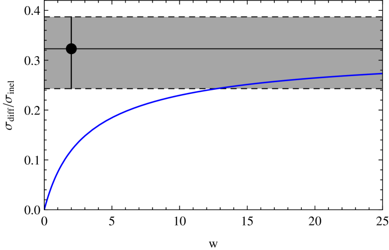
Figure 10: The point with the error bar is the measurement of the ratio $\sigma_{\rm diff}/\sigma_{\rm tot}$ obtained at $\sqrt{s}=7$ TeV by the ALICE collaboration alice-sigma . The line is the same ratio calculated in a multi–channel eikonal framework based on equation (53) as a function of the parameter $w$.

The results of a numerical calculation of $\sigma_{\rm diff}$ at $\sqrt{s}=7$ TeV using equation (57) are shown in fig. 10 in the form of the ratio $\sigma_{\rm diff}/\sigma_{\rm inel}$ plotted as a function of $w$, and compared to the ratio measured by ALICE alice-sigma : $\sigma_{\rm diff}/\sigma_{\rm inel}=0.32^{+0.064}_{-0.080}$. The diffractive cross sections vanishes for $w\to 0$ and grows monotonically with increasing $w$ going to the asymptotic value $\sigma_{\rm tot}/2-\sigma_{\rm el}$ for $w\to\infty$.

The experimental central value of the ratio $(\sigma_{\rm diff}+\sigma_{\rm el})/\sigma_{\rm tot}$ saturates the Pumplin bound. This corresponds to the limiting case $w\to\infty$, and therefore one can immediately see that from the study of the size of the diffractive cross section one can only derive a lower limit for $w$. At the 1 $\sigma$ level the limit is $w\geq 12.7$, and at 90% C.L. is $w>5.5$.

In lipari-lusignoli we argued that the data, including the results obtained at the $\overline{p}p$ colliders could be described, in the framework discussed in this section, with a constant value $w\simeq 3$. The LHC data does not support this hypothesis.

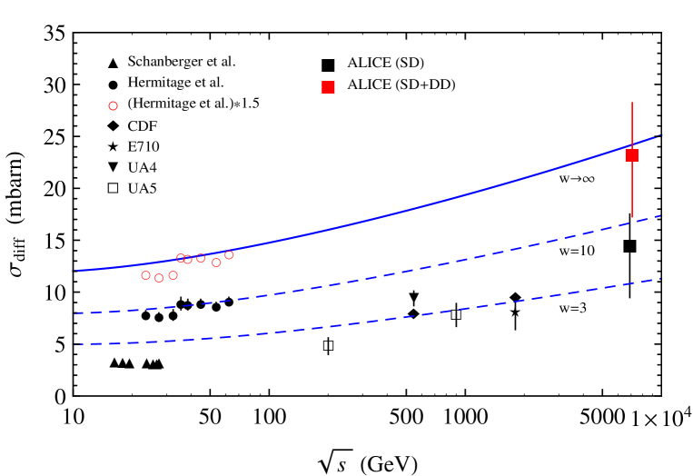
Figure 11: The smaller points are measurements of the single diffractive cross sections at ISR (Schamberger et al. Schamberger:1975ea and Armitage et al. Armitage:1981zp ), the $\overline{p}p$ colliders (UA4 Bernard:1986yh , UA5 Ansorge:1986xq , CDF Abe:1993wu and E710 Amos:1992jw ). The larger points are measurement of the single and diffractive cross sections at 7 TeV obtained combining the results of ALICE alice-sigma and TOTEM Antchev:2011vs . The lines calculation of the diffractive cross sections described in the main text.

The situation for the diffractive cross section as a function of energy is summarized in fig. 11 that shows the measurements of the diffractive cross section obtained at 7 TeV at LHC together with data on single diffraction obtained at ISR (where the results of Schamberger et al.Schamberger:1975ea and Armitage et al. Armitage:1981zp are in poor agreement with each other) and at $\overline{p}p$ collider energies (UA4 Bernard:1986yh , UA5 Ansorge:1986xq , CDF Abe:1993wu and E710 Amos:1992jw ). The ISR results refer to the kinematical region $M^{2}/s<0.1$, while the collider data refer to $M^{2}/s<0.05$. To compute the diffractive cross sections shown in the figure we have used the model described above, based on equation (53) with the eikonal function parametrized as in equation (17) with $A_{\chi}(b,s)$ of the form (20). The parameters $r_{0}(s)$ and $\sigma_{\rm eik}(s)$ have been calculated from the values of $\sigma_{\rm tot}(s)$ and $\sigma_{\rm el}(s)$ estimated with the fits to the total cross section from the PDG–2010 pdg-2010 and of the elastic cross section from Antchev:2011vs .

The prediction for the diffractive cross section we are discussing here, based on the Good and Walker ansatz, refers to the sum of the single and double diffraction cross section, on the other hand most of the data is only for single diffraction processes, because of the experimental difficulty in separating double diffraction from non–diffractive interactions. This introduces ambiguity in the interpretation. Inspecting fig. 11 one can see that a consistent interpretation of the data is not easy. An interesting speculation is that, allowing for systematic errors, and including a double diffraction cross section of order $\sigma_{\rm DD}\simeq\sigma_{\rm SD}/2$, the Miettinen–Pumplin bound is saturated at all energies for $s\gg 4\,m_{p}^{2}$.

In the simple model discussed here the single parameter $w$ completely determines the structure of the multi–channel eikonal, and allows to obtain the quantity $n(b,s)$ from the eikonal function, and so to make contact with a partonic description of the interaction. The relation between $\chi(b,s)$ and $n(b,s)$ was given in equation (54).

As discussed above the quantity $n(b,s)$ grows monotonically with $w$, diverging exponentially for $w$ large. This is problematic in a situation where the data suggests that $w$ is in fact large. A divergence of of $n(b,s)$ is not an immediately fatal problem since it does not imply the divergence of directly observable quantities, and in fact the QCD parton cross section are divergent in perturbation theory.

Equation (54) allows to compute the shape of the function $n(b,s)$ that has the physical meaning of the overlap of the hadronic matter distributions in the colliding hadrons. It is simple to see that in a multichannel eikonal framework the width of $n(b,s)$ is always narrower than the width of $\chi(b,s)$. In the scheme discussed here the width decreases monotonically with the increase of $w$.

Miettinen and Thomas Miettinen:1979ns , have estimated the spatial distribution of hadronic matter in the proton from the width of the eikonal function measured from the data on $pp$ scattering at ISR. In a single channel eikonal framework the width of the eikonal $\langle b^{2}\rangle_{\chi}\simeq 0.93$ fm suggests that hadronic matter has the same distribution of electric charge (see discussion in sec. III), but in multi–channel eikonal one has to conclude that hadronic matter has a significantly more compact distribution.

In the higher energy LHC data the eikonal function becomes broader, but also the parameter $w$ seems to grow, indicating that the interacting hadronic matter becomes more compact with increasing energy. This statement is in fact opposite to what one obtains in a single channel framework.

VI Discussion

It is natural to expect that the same fundamental dynamics determines the energy dependence of the total, elastic and diffractive cross section in $pp$ interactions and also controls the main properties of particle production in inelastic interactions such as multiplicity distributions, particle composition and inclusive energy spectra. From this idea it follows that it is not only desirable but necessary to construct a comprehensive and consistent theory that predicts the energy dependence of $\sigma_{\rm tot}$, $\sigma_{\rm el}$ and $\sigma_{\rm diff}$ and at the same time is the basis for a description of the final state in the collisions. It is also natural to expect that this comprehensive theory will be based on the partonic structure of colliding hadrons. Single and multi–channel eikonal models seems the most promising approaches for the construction of a parton–based model. In this work we have tried to interpret the cross sections measurements recently obtained at LHC in these frameworks.

The eikonal function $\chi(b,s)$ completely determines (and is completely determined by) the elastic scattering amplitude. Using the approximation that the amplitude is purely imaginary the eikonal function is real and can be calculated from the differential elastic cross section if the data cover a sufficiently broad range in momentum transfer $t$. In this work we have used the TOTEM data at 7 TeV to estimate the eikonal function. Comparing to the data on $pp$ scattering at lower energy, the eikonal function becomes larger and broader. The normalization of the eikonal function can be expressed as an eikonal cross section $\sigma_{\rm eik}(s)$ that grows from $55\pm 1$ mbarn at $\sqrt{s}=53$ GeV, to $156\pm 14$ mbarn at $\sqrt{s}=7$ TeV. The width of the eikonal (as measured by $\langle b^{2}\rangle_{\chi}$) grows from $0.86\pm 0.02$ fm to $1.19\pm 0.04$ fm.

In single channel eikonal models the eikonal cross section $\sigma_{\rm eik}(s)$ is interpreted as the total parton–parton cross section, while the shape in $b$ of $\chi(b,s)$ is the convolution of the spatial distributions of the interacting partons. A $\sqrt{s}=7$ TeV a cross section of order 150 mbarn corresponds, in a standard perturbative QCD calculation, to the cross section for (semi)–hard hadronic jet–pair production for $p_{\perp}^{2}\simeq 5$ GeV², and one expects that the total parton–cross section should be significantly larger. The identification of the parton and eikonal cross section that is the key element in a single channel eikonal framework is therefore problematic since $\sigma_{\rm parton}>\sigma_{\rm eik}$.

A possible solution is to introduce some modification of the standard calculation to reduce the parton cross section. This idea however encounters other difficulties when the eikonal framework is used as the basis for the multi–parton structure of inelastic events, a method that is in fact adopted in most of the Montecarlo event generator used to model the interactions at LHC. The general idea is that the complexity and average multiplicity of the final state grow with c.m. energy because the number of parton interactions per inelastic collision increases with $\sqrt{s}$. In a single channel eikonal framework the ratio $\sigma_{\rm eik}(s)/\sigma_{\rm inel}(s)$ has the physical meaning of the average number of parton interactions per collision. From the data one finds that the ratio $\sigma_{\rm eik}(s)/\sigma_{\rm inel}(s)$ increases from a value $1.55\pm 0.03$ at $\sqrt{s}=53$ GeV to $2.1\pm 0.2$ at 7 TeV. For the same c.m. energies the density of charged particles in the central region ($\left.dN/d\eta\right|_{\eta=0}$) grows significantly faster, from approximately 1.4 at $\sqrt{s}=53$ GeV to 6.1 at 7 TeV. For the event generators it is very difficult to reproduce this increase in average multiplicity respecting the constraint that the average number of interactions grows $\propto\sigma_{\rm eik}/\sigma_{\rm inel}$.

In view of these difficulties, we conclude that a single channel eikonal framework is not viable, and that it is necessary to consider a multi–channel model. This more complex framework is in fact desirable also because it has the very important theoretical merit to allow the inclusion of inelastic diffraction in a consistent way. In a multi–channel framework the eikonal cross section is not identified with the parton cross section but represents only a lower limit: $\sigma_{\rm eik}\leq\sigma_{\rm parton}$. This opens the possibility to solve the problems outlined above.

In a multi–channel framework the initial state is decomposed in a set of eigenstates that have distinct transmission amplitudes ($1-G_{j}$). The model is fully defined when all these transmission amplitudes are specified, respecting the condition that the weighted sum of the amplitudes reproduces the opacity function (see equation (33)). The diffractive cross section emerges when the distinct transmission amplitudes are different from each other, and is proportional to the dispersion of the distribution of the transition amplitudes. From the assumption that each amplitude is in the interval $0\leq G_{j}\leq 1$ it follows that the dispersion has a finite upper limit, and therefore the diffractive cross section has a maximum theoretically allowed value, the so called Miettinen Pumplin bound: $\sigma_{\rm diff}\leq\sigma_{\rm tot}/2-\sigma_{\rm el}$. The inequality is saturated when the transmission amplitudes take only the extreme values (zero or unity), in other words when all eigenstates in the Good–Walker decomposition are either completely absorbed or perfectly transparent.

The parton cross section is also calculable from the structure of the multi–channel model, and is related to the size of the diffractive cross section. It takes its minimum value ($\sigma_{\rm parton}=\sigma_{\rm eik}$) when the diffractive cross section vanishes, and grows monotonically with $\sigma_{\rm diff}$, diverging when the diffractive cross section approaches its maximum theoretically allowed value. It is remarkable that the combination of the TOTEM and ALICE data at $\sqrt{s}=7$ TeV is consistent with the saturation of the Miettinen Pumplin bound. This implies that the parton cross section is very large, and in fact divergent if the bound is saturated.

In this work we have discussed a “minimum model” to describe the multi–channel eikonal already discussed in the literature Miettinen:1979ns ; lipari-lusignoli . The model contains a single parameter ($w\geq 0$) that is proportional to the dispersion of the eigenvalues of the partial eikonals $\Omega_{j}$. Using this model one obtains a lower limit on $w$ that corresponds to a lower limit on the parton cross section of the order of $6\times 10^{6}$ mbarn (at 95% C.L.).

This result suggests that the parton cross section is in fact divergent. The divergence is not catastrophic, because it appears in the negative argument of an exponential, and it implies that a set of scattering eigenstates is absorbed with unit probability.

Acknowlegments. We are grateful to Lia Pancheri, Yogi Srivastava and Daniel Fagundes for many discussions on the problems discussed in this work.

Appendix A Parton interaction cross sections

In the theoretical framework we are considering, one introduces a “parton cross section” $\sigma_{\rm parton}(s)$ that is related to the total number of elementary interactions in $pp$ collisions. One must have that $\sigma_{\rm parton}(s)$ is larger than $\sigma_{\rm inel}(s)$ because in general in an inelastic $pp$ scattering one must have at least one such elementary interaction, and in fact the ratio $\sigma_{\rm parton}(s)/\sigma_{\rm inel}(s)$ has the physical meaning of the average number of elementary interactions per inelastic event. The calculation of the quantity $\sigma_{\rm parton}(s)$ is a non trivial problem, because the parton–parton cross sections (calculated at tree level) diverge for low momentum transfer, when in fact perturbation theory fails. Several authors have dealt with this problem decomposing $\sigma_{\rm parton}(s)$ in a “hard” (calculable in perturbation theory) and a “soft” component that is estimated with different methods.

In this appendix we want to evaluate the cross section for parton–parton hard scattering in $pp$ collisions, in the region where one can be confident that a perturbative calculation is valid. For example, the differential cross section for elastic gluon–gluon scattering can be calculated in perturbation theory convoluting the gluon distribution functions with the elementary cross section for gluon–gluon scattering with the result:

$$\frac{d^{3}\sigma_{gg\to gg}}{dt\,dx_{1}\,dx_{2}}(t,x_{1},x_{2};\sqrt{s})=~{}f_{g}(x_{1},|t|)~{}f_{g}(x_{2},|t|)~{}\frac{d\hat{\sigma}_{gg\to gg}}{dt}(t,\hat{s})$$ (58)

where $x_{1}$ and $x_{2}$ are the fractional momenta carried by the gluons in the colliding protons and $\hat{s}=s\,x_{1}\,x_{2}$. It is then possible to obtain the cross section $\sigma_{gg}(s,|t_{\rm min}|)$ for all gluon–gluon scatterings with momentum transfer larger than $-t_{\rm min}$, integrating the expression above over the appropriate kinematical range.

$$\sigma_{gg}(s,t_{\rm min}) = \int dx_{1}~{}\int dx_{2}~{}\int d|t|~{}\theta\left(x_{1}\,x_{2}-\frac{2|t|}{s}\right)~{}\theta(|t|-|t_{\rm min}|)\times~{}~{}~{}~{}$$ (59)

$$~{}~{}~{}~{}~{}~{}~{}~{}~{}f_{g}(x_{1},|t|)\;f_{g}(x_{2},|t|)~{}\frac{d\hat{\sigma}_{gg}}{dt}(t,\hat{s})$$

Similarly one can compute cross sections for quark–gluon and quark–quark scattering. Combining these results one can obtain the hard cross section as the combination of $gg$, $qg$ and $qq$ scatterings:

$$\sigma_{\rm hard}(s,|t_{\rm min}|)=\sigma_{gg}+\sigma_{qg}+\sigma_{qq}$$ (60)

The cross sections for hard parton scattering scale approximately as $|t_{\rm min}|^{-1}$, reflecting the divergence ($\propto t^{-2}$) of the parton–parton differential elastic cross section, and grows rapidly with $s$, because with increasing energy the hard scattering of partons with lower $x$ ($x_{1}\,x_{2}\geq 2\,|t_{\rm min}|/s$) becomes kinematically possible.

To obtain numerical estimates of $\sigma_{\rm hard}(s,|t_{\rm min}|)$ we have used the Leading Order PDF’s of Martin, Roberts, Stirling, Thorne and Watt (MRSTW) Martin:2009iq . The results of the calculation are shown in fig. 6 as a function of the $|t_{\rm min}|$ cut for fixed values of $\sqrt{s}=53$, 546 and 7000 GeV.

At the LHC energy ($\sqrt{s}=7$ TeV), the hard parton scattering cross section is $\sigma_{\rm hard}=1465$ mbarn for $|t_{\rm min}|=2$ GeV², decreasing to 162 mbarn for $|t_{\rm min}|=10$ GeV².

For a qualitative understanding one can observe that using some approximations it is possible to obtain an analytic expressions for the cross sections for hard parton scattering.

The elementary differential cross section for gluon–gluon scattering has the form:

$$\frac{d\hat{\sigma}_{gg}}{dt}(t,\hat{s}) = \frac{9\,\pi}{2}\,\frac{\alpha_{s}^{2}(|t|)}{\hat{s}^{2}}\;\left[3-\frac{t\,u}{\hat{s}^{2}}-\frac{\hat{s}\,u}{t^{2}}-\frac{\hat{s}\,t}{u^{2}}\right]$$ (61)

$$\simeq \frac{9\,\pi}{2}\,\frac{\alpha_{s}^{2}(|t|)}{t^{2}}~{}\left[1+O\left(\frac{t}{\hat{s}}\right)\right]$$

that diverges as $t^{-2}$ for $t\to 0$. The integration over $t$ can be performed analytically if one neglects the scale dependence of $\alpha_{s}$. The result is:

$$\hat{\sigma}_{gg}(\hat{s},|t_{\rm min}|) = \frac{9\pi}{2}\,\frac{\alpha_{s}^{2}}{|t_{\rm min}|}~{}F_{\rm kin}\left(\frac{2|t_{\rm min}|}{\hat{s}}\right)$$ (62)

$$= \hat{\sigma}_{gg}^{\rm asy}(|t_{\rm min}|)~{}F_{\rm kin}\left(\frac{2|t_{\rm min}|}{\hat{s}}\right)~{}.$$

The function $F_{\rm kin}(\hat{\tau})$ is a kinematical suppression factor that takes into account the available phase space (with $\hat{\tau}=2|t_{\rm min}|/\hat{s}$). It vanishes at the threshold ($\hat{\tau}=1$) and is equal to unity for $\hat{\tau}=0$ (that corresponds to $\hat{s}\to\infty$). The exact expression for $F_{\rm kin}(\hat{\tau})$ is:

$$F_{\rm kin}(\hat{\tau})=1-\hat{\tau}\left[\frac{(20-106\,\hat{\tau}+42\,\hat{\tau}^{2}-5\,\hat{\tau}^{3}+\hat{\tau}^{4})}{48\,(2-\hat{\tau})}+\frac{1}{2}\;\log\left(\frac{2}{\hat{\tau}}-1\right)\right]$$ (63)

For numerical purposes this can be approximated with the simple form: $f(\hat{\tau})\simeq(1-\hat{\tau})$ that has correct values for $\hat{\tau}=0$ (large $\hat{s}$ limit) and $\hat{\tau}=1$ (threshold).

Neglecting the scale dependence of the PDF’s, one can perform the $t$ integration in (59) and the $gg$ scattering cross section results factorized in the form:

$$\sigma_{gg}(s,t_{\rm min})\simeq\hat{\sigma}_{gg}^{\rm asy}(|t_{\rm min}|)\times C_{gg}(\tau)$$ (64)

(with $\tau=2|t_{\rm min}|/s$) that is the product of the (asymptotic) elementary gluon–gluon cross section with the convolution of the gluons PDF’s $C_{gg}(\tau)$ that computes the the number of gluon pairs above threshold (that is with $x_{1}x_{2}>\tau$), with the function $F_{\rm kin}[\hat{\tau}=\tau/(x_{1}\,x_{2})]$ that takes into account the phase space available for the scattering:

$$C_{gg}(\tau) = \int dx_{1}\int dx_{2}~{}\theta\left(x_{1}\,x_{2}-\frac{2|t_{\rm min}|}{s}\right)\times~{}~{}~{}~{}$$

$$~{}~{}~{}~{}f_{g}(x_{1},|t_{\rm min}|)\;f_{g}(x_{2},|t_{\rm min}|)~{}F_{\rm kin}\left(\frac{\tau}{x_{1}x_{2}}\right)$$

If the gluon PDF’s are approximated with the simple form $f_{g}(x)=K_{g}/x^{1+\varepsilon}$, the convolution factor can be calculated explicitely:

$$C_{gg}(\tau)=K_{g}^{2}\left[-\frac{\tau^{-\varepsilon}\;\log\tau}{\varepsilon\,(1+\varepsilon)}-\frac{1+2\,\varepsilon+\varepsilon^{2}\,(1-\tau)-\tau^{-\varepsilon}\,(1-2\,\varepsilon)}{\varepsilon^{2}(1+\varepsilon)^{2}}\right]$$ (65)

In the limit of $\varepsilon\to 0$ the convolution factor becomes:

$$C_{gg}(\tau)\simeq K_{g}^{2}\;\left[\frac{\log^{2}\tau}{2}+\log\tau+1-\tau\right]\;.$$ (66)

In the limit of high energy ($s/(2|t_{\rm min}|)\gg 1$, or $\tau\to 0$) their asymptotic behavior is:

$$C_{gg}\simeq K_{g}^{2}~{}\frac{1}{\varepsilon}\;\left(\frac{s}{2\,|t_{\rm min}|}\right)^{\varepsilon}\log\left(\frac{s}{2\,|t_{\rm min}|}\right)$$ (67)

or for $\varepsilon\to 0$:

$$C_{gg}\simeq K_{g}^{2}\;\frac{1}{2}~{}\log^{2}\left(\frac{s}{2\,|t_{\rm min}|}\right)$$ (68)

The cross sections for quark–gluon and quark–quark scattering can be written as similar decompositions, noting that the asymptotic behavior of elementary cross sections differ by simple color factors:

$$\hat{\sigma}_{gg}^{\rm asy}=\frac{9}{4}\;\hat{\sigma}_{qg}^{\rm asy}=\left(\frac{9}{4}\right)^{2}\;\hat{\sigma}_{qq}^{\rm asy}~{}.$$ (69)

Appendix B The functions $p(\alpha)$ and $p_{G}(G)$

In a multi–channel eikonal model the opacity function $\Gamma(b,s)$ is decomposed into partial components as:

$$\Gamma=\sum_{j}p_{j}~{}G_{j}$$ (70)

(where we have left implicit the $b$ and $s$ dependence). The partial opacities $G_{j}(b,s)$ are assumed to be real and in the interval $[0,1]$, therefore in the most general case one has to consider a continuous infinity of states that can be labeled with the eigenvalue $G$. The decomposition (70) can then be written as the integral:

$$\Gamma=\int_{0}^{1}dG~{}p_{G}(G)~{}G=\left\langle G\right\rangle$$ (71)

(where the probability distribution $p_{G}(G)$ is normalized). The discrete case can be recovered using for the function $p_{G}(G)$:

$$p_{G}(G)=\sum_{j}p_{j}~{}\delta[G-G_{j}]~{}.$$ (72)

One can relate $G$ to the parameter $\alpha$ with the relation

$$G=1-e^{-\Omega}=1-e^{-\langle\Omega\rangle\,\alpha}~{}.$$ (73)

Since $\langle\Omega\rangle$ is positive, and $G$ can vary in the interval $[0,1]$, the quantity $\alpha$ takes values in the interval $0\leq\alpha<\infty$. The decomposition of the profile function can then be rewritten in the form:

$$\Gamma=\int_{0}^{\infty}d\alpha~{}p(\alpha)~{}\left(1-e^{-\langle\Omega\rangle\;\alpha}\right)~{}.$$ (74)

The probability distribution of $\alpha$ is normalized to unity and satisfies the constraint:

$$\int_{0}^{\infty}d\alpha~{}\alpha~{}p(\alpha)=1~{}.$$ (75)

As discussed in the main text, one can make the interpretation: $\langle\Omega\rangle=n/2$ where $n$ is the average number of parton interactions.

The two decompositions of the opacity functions in equations (71) and (50) are equivalent. There is a one–to–one correspondence between $G$ and $\alpha$, and one can obtain $p(\alpha)$ fron $p_{G}(G)$ or viceversa. Equation (74) determines implicitely $\langle\Omega\rangle$ from $\Gamma$ (or viceversa $\Gamma$ from $\langle\Omega\rangle$) if the function $p(\alpha)$ (or $p_{G}(G)$) is known.

The important quantity $\langle G^{2}\rangle$ that enters the expression for the diffractive and absorption cross sections (see equations (36) and (39)) can be calculated in the two decompositions as:

$$\langle G^{2}\rangle = \int_{0}^{1}dG~{}p_{G}(G)~{}G^{2}$$ (76)

$$\langle G^{2}\rangle = \int_{0}^{\infty}d\alpha~{}p(\alpha)~{}\left(1-e^{-\langle\Omega\rangle\;\alpha}\right)^{2}$$ (77)

In this work we have used for $p(\alpha)$ the form

$$p(\alpha)=\frac{1}{w\;\Gamma_{\rm E}\left(\frac{1}{w}\right)}~{}\left(\frac{\alpha}{w}\right)^{\frac{1}{w}-1}\exp\left[-\frac{\alpha}{w}\right]$$ (78)

(aso given in the main text in equation (53)) that depends on the parameter $w\geq 0$. For $n$ integer one has:

$$\left\langle\alpha^{n}\right\rangle=\int_{0}^{\infty}d\alpha\;p(\alpha)\;\alpha^{n}=(1+w)\,(1+2w)\ldots[1+(n-1)w]$$ (79)

so the distribution is normalized, satisfies equation (52) and $w$ is the variance of the distribution ($\langle\alpha^{2}\rangle=1+w$).

The function (78) has the attractive property that when the parameter $w$ spans the interval $0\leq w<\infty$ the quantity $\langle G^{2}\rangle$ spans the entire interval of the theoretically allowed values. For $w=0$ one has $\langle G^{2}\rangle=\Gamma^{2}$, and the value of $\langle G^{2}\rangle$ grows monotonically with $w$, reaching (for $w\to\infty$) the asymptotic value $\langle G^{2}\rangle\to\Gamma$.

The qualitative features of the distributions change with $w$.

• In the limit of $w\to 0$ the distributions $p(\alpha)$ and $p_{G}(G)$ become delta functions: $p(\alpha)=\delta[\alpha-1]$ and $p_{G}(G)=\delta[G-\Gamma]$

• For $w$ small, the distribution $p(\alpha)$ is approximately a gaussian of width $\sigma=\sqrt{w}$ centered at $\alpha\simeq 1$ while $p_{G}(G)$ is a narrow distribution centered on $G\simeq\Gamma$.

• For $0<w<1$ the distributions $p(\alpha)$ and $p_{G}(G)$ have one single maximum. For $p(\alpha)$ the maximum is at $\alpha=1-w$, the positions of the maximum for $p_{G}(G)$ depends on $\Gamma$ and $w$.

• For $w=1$ the $p(\alpha)$ distribution is equal to $e^{-\alpha}$ while $p_{G}(G)$ depends monotonically on $G$ with maximum at $G=0$ ($G=1$) for $\Gamma<1/2$ ($\Gamma>1/2$) (for $\Gamma=1/2$ the distribution is flat).

• For $w>1$ the $p(\alpha)$ distribution diverges when $\alpha\to 0$, and decreases monotonically. The corresponding $p_{G}(G)$ has divergence for both $G\to 0$ and $G\to 1$ and a single minimum in the center. When $w\gg 1$ the probability is concentrated in two small intervals close to $G\simeq 0$ and $G\simeq 1$, and is always very small in the remaining central part of the interval $[0,1]$.

• In the limit $w\to\infty$ the function $p_{G}(G)$ takes the asymptotic form:

  $$p_{G}(G)=(1-\Gamma)~{}\delta(G)+\Gamma~{}\delta(1-G)$$ (80)

  that corresponds to complete transparency or complete absorption.

The general form of $p_{G}(G)$ for an arbitrary value of $w$ is:

$$p_{G}(G)=\frac{[(1-\Gamma)^{-w}-1]^{-1/w}}{\Gamma_{\rm E}(1/w)}\left[-\ln(1-G)\right]^{-1+1/w}~{}\left[1-G\right]^{-1+1/((1-\Gamma)^{-w}-1)}\;,$$ (81)

for large $w$ this becomes approximately

$$p_{G}(G)\propto\left[-\ln(1-G)\right]^{-1}~{}\left[1-G\right]^{-1}$$ (82)

with divergences at $G=0$ and $G=1$.

Figure 1: Measurements of the elastic cross section in $pp$ collisions at $\sqrt{s}=7$ TeV obtained by the TOTEM collaboration Antchev:2011vs ; totem-a ; Antchev:2011zz . The line is a fit to the data.

Figure 2: Measurements of the elastic cross section in $pp$ collisions at $\sqrt{s}=53$ GeV obtained at ISR Nagy:1978iw ; Ambrosio:1982zj ; Breakstone:1984te . The line is a fit to the data.

Figure 3: Opacity functions $\Gamma(b,s)$ calculated from the measurements of the differential elastic cross sections in $pp$ collisions at $\sqrt{s}=53$ and 7000 GeV. The opacity functions are obtained from the fits to the data shown fig. 1 and 2 using equation (16). The corresponding eikonal functions are shown in fig. 4.

Figure 4: Shape of the eikonal function $A_{\chi}(b,s)=2\,\chi(b,s)/\sigma_{\rm eik}(s)$ at $\sqrt{s}=53$ GeV and 7 TeV. The eikonal function was obtained from the fits to the data on elastic scattering shown in fig. 1 and 2. The corresponding opacity functions are shown in fig. 3.

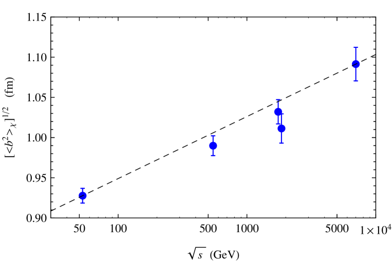
Figure 7: Estimates of the quantity $\sqrt{\langle b^{2}\rangle_{\chi}}=4\,r_{0}$ obtained from measurements of $\sigma_{\rm tot}$ and $B$ at the same c.m. energy. The dashed line is a fit of form $a+b\;\ln s$ drawn to guide the eye.

Figure 8: Plot of the relation between $\sigma_{\rm tot}$ and the slope $B$. The (red) disks are measurements for $pp$ scattering at ISR ($\sqrt{s}=53$ GeV) and LHC ($\sqrt{s}=7$ TeV); the (black) squares are measurements for $\overline{p}p$ scattering at CERN ($\sqrt{s}=546$ GeV) and Fermilab ($\sqrt{s}=1.8$ TeV). The lines describe the relation when the eikonal function has the $b$ dependence of equation (20) with the parameter $r_{0}$ given by $1$, 1.1 and 1.2 times $R_{p}$ (with $R_{p}=0.234$ fm obtained from the electromagnetic form factor).

References

- (1) G. Antchev et al. [Totem Collaboration], Europhys. Lett. 96, 21002 (2011) [arXiv:1110.1395 [hep-ex]].
- (2) G. Antchev et al. [TOTEM Collaboration], Europhys. Lett. 101, 21002 (2013).
- (3) G. Antchev et al. [Totem Collaboration], Europhys. Lett. 95, 41001 (2011) [arXiv:1110.1385 [hep-ex]].
- (4) G. Antchev et al. [The TOTEM Collaboration], Europhys. Lett. 101, 21003 (2013).
- (5) G. Antchev et al. [The TOTEM Collaboration], Europhys. Lett. 101, 21004 (2013).
- (6) G. Antchev et al. [Totem Collaboration], preprint CERN-PH-EP-2012-354 (2012).
- (7) B. Abelev et al. [The ALICE Collaboration], arXiv:1208.4968 [hep-ex].
- (8) G. Aad et al. [ATLAS Collaboration], Nature Commun. 2, 463 (2011) [arXiv:1104.0326 [hep-ex]].
- (9) S. Chatrchyan et al. [CMS Collaboration], Phys. Lett. B 722, 5 (2013) [arXiv:1210.6718 [hep-ex]].
- (10) H. I. Miettinen and J. Pumplin, Phys. Rev. D 18, 1696 (1978).
- (11) O. Adriani et al., Phys. Lett. B 703, 128 (2011) [arXiv:1104.5294 [hep-ex]].
- (12) M. G. Ryskin, A. D. Martin and V. A. Khoze, Eur. Phys. J. C 72, 1937 (2012) [arXiv:1201.6298 [hep-ph]].
- (13) E. Gotsman, E. Levin and U. Maor, Phys. Rev. D 85, 094007 (2012) [arXiv:1203.2419 [hep-ph]].
- (14) E. Gotsman, E. Levin and U. Maor, Phys. Lett. B 716, 425 (2012) [arXiv:1208.0898 [hep-ph]].
- (15) A. Grau, S. Pacetti, G. Pancheri and Y. N. Srivastava, Phys. Lett. B 714, 70 (2012) [arXiv:1206.1076 [hep-ph]].
- (16) B. Z. Kopeliovich, I. K. Potashnikova and B. Povh, Phys. Rev. D 86, 051502 (2012) [arXiv:1208.5446 [hep-ph]].
- (17) D. A. Fagundes, M. J. Menon and P. V. R. G. Silva, J. Phys. G 40, 065005 (2013) [arXiv:1208.3456 [hep-ph]].
- (18) E. Nagy et al. Nucl. Phys. B150, 221 (1979).
- (19) M. Ambrosio et al. Phys. Lett. B 115, 495 (1982).
- (20) A. Breakstone et al. Nucl. Phys. B248, 253-260 (1984).
- (21) J. R. Cudell et al. [COMPETE Collaboration], Phys. Rev. Lett. 89, 201801 (2002) [hep-ph/0206172].
- (22) L. Durand and H. Pi, Phys. Rev. D 38, 78 (1988).
- (23) F. Abe et al. [CDF Collaboration], Phys. Rev. D 50, 5518 (1994).
- (24) F. Abe et al. [CDF Collaboration], Phys. Rev. D 50, 5550 (1994).
- (25) C. Avila et al. [E811 Collaboration], Phys. Lett. B 445, 419 (1999).
- (26) T. K. Gaisser and F. Halzen, Phys. Rev. Lett. 54, 1754 (1985).
- (27) G. Pancheri and Y. Srivastava, Phys. Lett. B159, 69 (1985).
- (28) A. D. Martin, W. J. Stirling, R. S. Thorne and G. Watt, Eur. Phys. J. C 63, 189 (2009) [arXiv:0901.0002 [hep-ph]].
- (29) T. Sjostrand and M. van Zijl, Phys. Rev. D 36, 2019 (1987).
- (30) L. Durand and H. Pi, Phys. Rev. D 40, 1436 (1989).
- (31) M. M. Block and F. Halzen, Phys. Rev. D 72, 036006 (2005) [Erratum-ibid. D 72, 039902 (2005)] [hep-ph/0506031].
- (32) R. Corke and T. Sjöstrand, JHEP 1105, 009 (2011) [arXiv:1101.5953 [hep-ph]].
- (33) M. L. Good and W. D. Walker, Phys. Rev. 120, 1857 (1960).
- (34) P. Lipari and M. Lusignoli, Phys. Rev. D 80, 074014 (2009) [arXiv:0908.0495 [hep-ph]].
- (35) H. I. Miettinen and G. H. Thomas, Nucl. Phys. B 166, 365 (1980).
- (36) R. D. Schamberger, J. Lee-Franzini, R. Mccarthy, S. Childress and P. Franzini, Phys. Rev. Lett. 34, 1121 (1975).
- (37) J. C. M. Armitage et al., Nucl. Phys. B 194, 365 (1982).
- (38) D. Bernard et al. [UA4 Collaboration], Phys. Lett. B 186, 227 (1987).
- (39) R. E. Ansorge et al. [UA5 Collaboration], Z. Phys. C 33, 175 (1986).
- (40) N. A. Amos et al. [E710 Collaboration], Phys. Lett. B 301, 313 (1993).
- (41) F. Abe et al. [CDF Collaboration], Phys. Rev. D 50, 5535 (1994).
- (42) K. Nakamura et al. [Particle Data Group Collaboration], J. Phys. G 37, 075021 (2010).