The kaon semileptonic form factor with near physical domain wall quarks
Abstract
We present a new calculation of the semileptonic form factor at zero momentum transfer in domain wall lattice QCD with dynamical quark flavours. By using partially twisted boundary conditions we simulate directly at the phenomenologically relevant point of zero momentum transfer. We perform a joint analysis for all available ensembles which include three different lattice spacings ( = 0.09 – 0.14 fm), large physical volumes () and pion masses as low as 171 MeV. The comprehensive set of simulation points allows for a detailed study of systematic effects leading to the prediction , where the first error is statistical and the second error systematic. The result allows us to extract the CKM-matrix element and confirm first-row CKM-unitarity in the Standard Model at the sub per mille level.
Keywords:
lattice QCD, kaons, semileptonic decays, CKM test1 Introduction
In the Standard Model (SM), the unitary Cabibbo-Kobayashi-Maskawa (CKM) matrix parametrises the relative strength of different flavour-changing weak processes. Inconsistencies in the CKM-picture would indicate the presence of new physics beyond the SM. It is therefore important to determine all CKM-matrix elements as precisely as possible by studying flavour changing processes both experimentally (e.g. at the NA62 and LHCb experiments at CERN) and theoretically.
In this paper we discuss the determination of the matrix element from the study of semileptonic kaon () decays and the test of the unitarity of the first row of the CKM matrix . is very small, O, compared to the current uncertainties in and . The matrix element is known very precisely from neutron -decay Hardy:2008gy and reaching comparable precision for is crucial in searching for deviations from CKM-unitarity and for possible signs of new physics. This can be achieved by combining lattice results for the form factor with from the phenomenological analysis Antonelli:2010yf of experimental results. Note that can also be determined from the experimental measurement of pion and kaon leptonic decays and lattice results for the ratio of decay constants (cf. FLAG Colangelo:2010et ).
The field-theoretical and technical tools developed in the series of papers Hashimoto:1999yp ; Becirevic:2004ya ; Boyle:2007wg ; Boyle:2010bh have enabled the calculation of in lattice computations with a precision of around 0.5% Lubicz:2009ht ; Boyle:2007qe ; Boyle:2010bh ; Kaneko:2011rp ; Bazavov:2012cd . The current experimental uncertainty in is about 0.2%, with an anticipated further reduction of about in this uncertainty from the KLOE-2-experiment AmelinoCamelia:2010me . These results challenge lattice simulations to achieve a similar precision.
In our previous work Boyle:2007qe ; Boyle:2010bh we have shown that a precision of 0.5% can indeed be achieved in practice. We have also removed one of the dominant sources of systematic error by using the method of partially-twisted boundary conditions (explained below) to avoid an interpolation in the momentum transfer to the point Boyle:2007wg ; Boyle:2010bh . Other collaborations have computed the form factor in lattice QCD with Tsutsui:2005cj ; Dawson:2006qc ; Lubicz:2009ht ; Lubicz:2010bv and Kaneko:2011rp ; Bazavov:2012cd dynamical quarks and an overview of the world data can be found in the FLAG report Colangelo:2010et . The distinct features of our new calculations are results for three values of the lattice spacing (a = 0.09 fm – 0.14 fm), lighter simulated quark masses (MeV) Arthur:2012opa than used in previous calculations and simulations in large volume () using partially twisted boundary conditions.
In the remainder of the paper we present the details of the calculation, but here we anticipate the final result. The comprehensive set of simulation points allows for a detailed study of systematic effects leading to the result:
| (1) |
where in the result for the form factor the first error is statistical and the second error systematic. Our result for the CKM matrix element allows for the confirmation of first-row CKM-unitarity in the Standard Model at the sub per mille level.
In the following we start with a discussion of the techniques used to determine the form factor in terms of Euclidean correlation functions. We then explain our choice of simulation parameters, followed by a description of the calculation itself, the extrapolation of the lattice data to the physical point and the error budget for final results. Finally we present our conclusions.
2 Calculational procedure
The matrix element of the vector current between initial and final pseudoscalar states and decomposes into two form factors,
| (2) |
where is the momentum transfer. For semileptonic decay, , and . The scalar form factor is defined by
| (3) |
and satisfies .
In order to simulate directly at , we use partially twisted boundary conditions Sachrajda:2004mi ; Bedaque:2004ax , combining gauge field configurations generated using sea quarks obeying periodic spatial boundary conditions with valence quarks obeying twisted boundary conditions. Specifically, the valence quarks satisfy boundary conditions of the form:
| (4) |
where is either a strange quark or one of the degenerate up and down quarks. The dispersion relation for a meson in cubic volume projected onto Fourier momentum takes the form deDivitiis:2004kq ; Flynn:2005in ,
| (5) |
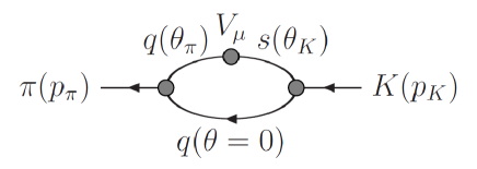
where is the energy, is the meson’s mass and is the difference of the twist angles for the two valence quarks in the meson. By varying the twist angles, arbitrary momenta can be reached. Here we choose the angles such that . In the quark flow diagram of Figure 1, we twist the strange () and light quarks () coupling to the vector current with phases and in order to give momenta to the kaon and pion respectively. The choice of twisting angles is discussed further in Section 3 and their values are given in Table 2.
The matrix element in (2) can be extracted from the time dependence of combinations of Euclidean two- and three-point correlation functions in lattice QCD. The two-point function is defined by
| (6) |
where or , and are pseudoscalar interpolating operators for the corresponding mesons, and . We assume that and (where is the temporal extent of the lattice) are large enough that the correlation function is dominated by the lightest state (i.e. the pion or kaon). The constants are given by . The three-point functions are defined by
| (7) | ||||
where is a pion or a kaon, is the vector current with flavour quantum numbers to allow the transition and we have defined . The constant satisfies (time-direction) and for . Again we assume that all time intervals are sufficiently large for the lightest hadrons to give the dominant contribution.
We obtain the vector current renormalisation factor as follows. For illustration, take , in which case is defined by
| (8) |
In the numerator we use the function where and are determined by fitting and applying (5). The superscript in the denominator indicates that we take the bare (unrenormalised) current in the three-point function.
In the following we drop the labels and in the three-point functions (since they are fixed) and we combine the two- and three- point functions into the ratios
| (9) | ||||
which are constructed such that
| (10) |
for . For the ratios we use the naming convention of Boyle:2007wg .
Once these ratios have been computed for several choices for and while keeping constant at zero the form factor can be obtained as the solution of the corresponding system of linear equations.
3 Simulation parameters
We use ensembles of gauge fields with dynamical flavours at three different lattice spacings, . The basic parameters of these ensembles are listed in Table 1. On the finer lattices (smaller lattice spacings) we use the Iwasaki gauge action Iwasaki:1984cj ; Iwasaki:1985we and the domain wall fermion (DWF) action Kaplan:1992bt ; Shamir:1993zy . Two of the ensembles are generated with labelled C in the following, ) Aoki:2010dy and labelled A in the following, Allton:2008pn , with lattice sizes and respectively, with the extent of the fifth dimension in both cases. On these ensembles we have simulated with unitary pion masses down to Allton:2008pn ; Aoki:2010dy . To reach lower unitary pion masses, as low as Arthur:2012opa , we have used an additional third set of ensembles that employs the Iwasaki gauge action with an additional weighting factor, the ‘dislocation suppressing determinant ratio’ (DSDR) in the path integral to suppress gauge configurations with localised instanton-like artifacts. The dislocations support additional low-modes of the Dirac operator and suppressing them helps reduce the growth of the residual mass (which parameterises the explicit chiral symmetry breaking arising from the finite fifth dimension) on this coarser lattice. The Iwasaki-DSDR ensembles are generated at labelled B, GeV, with lattice size and . On all ensembles the spatial volumes are large enough to ensure for all simulated masses, keeping finite-volume corrections small. More details on all these ensembles and results for a variety of light hadronic quantities are given in Allton:2007hx ; Allton:2008pn ; Aoki:2010dy ; Aoki:2010pe ; Arthur:2012opa . We note that owing to the change in action, cutoff-effects which start at for DWF will behave differently for ensemble B than for A and C Arthur:2012opa . This will be discussed further in Section 5.
| action | |||||||||||||
|---|---|---|---|---|---|---|---|---|---|---|---|---|---|
| set | sea | val | /MeV | ||||||||||
| A3 | DWF | DWF | 2.13 | 0.11 | 24 | 64 | 0.0300 | 0.040 | 0.040 | 678 | 2 | 105 | 9.3 |
| A2 | DWF | DWF | 2.13 | 0.11 | 24 | 64 | 0.0200 | 0.040 | 0.040 | 563 | 2 | 85 | 7.7 |
| A1 | DWF | DWF | 2.13 | 0.11 | 24 | 64 | 0.0100 | 0.040 | 0.040 | 422 | 2 | 153 | 5.8 |
| A | DWF | DWF | 2.13 | 0.11 | 24 | 64 | 0.0050 | 0.040 | 0.040 | 334 | 8 | 143 | 4.6 |
| A | DWF | DWF | 2.13 | 0.11 | 24 | 64 | 0.0050 | 0.040 | 0.030 | 334 | 8 | 143 | 4.6 |
| C8 | DWF | DWF | 2.25 | 0.09 | 32 | 64 | 0.0080 | 0.030 | 0.025 | 398 | 8 | 120 | 5.5 |
| C6 | DWF | DWF | 2.25 | 0.09 | 32 | 64 | 0.0060 | 0.030 | 0.025 | 349 | 8 | 153 | 4.8 |
| C4 | DWF | DWF | 2.25 | 0.09 | 32 | 64 | 0.0040 | 0.030 | 0.025 | 295 | 9 | 135 | 4.1 |
| B42 | DSDR | DWF | 1.75 | 0.14 | 32 | 64 | 0.0042 | 0.045 | 0.045 | 248 | 16 | 162 | 5.7 |
| B1 | DSDR | DWF | 1.75 | 0.14 | 32 | 64 | 0.0010 | 0.045 | 0.045 | 171 | 16 | 196 | 3.9 |
For the computation of the form factor we distinguish two different kinematical situations. We denote by ‘kinematics I’ the case where either the kaon or the pion are at rest Boyle:2007wg :
| (11) | ||||
| (12) |
In some cases, we twist in more than one direction. This increases the number of equations from which we can determine the form factors in (2). It may also reduce discretisation errors coming from and higher powers, where is a component of the momentum. On the coarsest lattice, twisting only the kaon leads to large twisting angles, giving the kaon a momentum of order of a typical Fourier momentum unit, . Therefore, in ‘kinematics II’ we choose two components of the kaon twisting angle to be non-zero but not too large and then fix the twist of the pion in the remaining direction to ensure that . Our complete set of twisting angles is summarised in Table 2.
| kinematics I | kinematics II | |||||||||||
|---|---|---|---|---|---|---|---|---|---|---|---|---|
| set | ||||||||||||
| A3 | (0.375, | 0.375, | 0.375) | (0.402, | 0.402, | 0.402) | na. | na. | ||||
| A2 | (0.790, | 0.790, | 0.790) | (0.943, | 0.943, | 0.943) | na. | na. | ||||
| A1 | (1.270, | 1.270, | 1.270) | (1.842, | 1.842, | 1.842) | na. | na. | ||||
| A | (2.682, | 0.000, | 0.000) | (4.681, | 0.000, | 0.000) | na. | na. | ||||
| A | (2.129, | 0.000, | 0.000) | (3.337, | 0.000, | 0.000) | na. | na. | ||||
| C8 | (0.943, | 1.622, | 0.000) | (0.000, | 1.570, | 2.094) | na. | na. | ||||
| C6 | (0.943, | 1.934, | 0.000) | (0.000, | 1.570, | 2.915) | na. | na. | ||||
| C4 | (1.739, | 1.739, | 0.000) | (0.000, | 3.086, | 3.086) | na. | na. | ||||
| B42 | (3.209, | 0.000, | 3.209) | (0.000, | 6.587, | 6.587) | (3.689, | 0.000, | 0.000) | (0.000, | 2.356, | 3.927) |
| B1 | (2.513, | 4.382, | 0.000) | (0.000, | 0.000, | 0.000) | (0.000, | 0.000, | 4.173) | (4.712, | 3.142, | 0.000) |
| set | |||
|---|---|---|---|
| A3 | 0.38838(39) | 0.41626(39) | 0.9992(1) |
| A2 | 0.32234(47) | 0.38437(48) | 0.9956(4) |
| A1 | 0.24157(40) | 0.35009(41) | 0.9870(9) |
| A | 0.19093(45) | 0.33198(58) | 0.9760(43) |
| A | 0.19093(45) | 0.29819(52) | 0.9858(28) |
| C8 | 0.17247(49) | 0.24123(47) | 0.9904(17) |
| C6 | 0.15105(44) | 0.23274(47) | 0.9845(23) |
| C4 | 0.12776(43) | 0.22623(54) | 0.9826(35) |
| B42 | 0.18067(19) | 0.37157(29) | 0.9771(21) |
| B1 | 0.12455(20) | 0.35920(31) | 0.9710(45) |
4 Numerical results
We have used the bootstrap procedure efron:1979 with 500 bootstrap samples for each ensemble. The choice of binning is based on previous auto-correlation studies in Allton:2008pn ; Aoki:2010dy ; Arthur:2012opa . We have combined the measurements for noise source positions (cf. Table 1) into one bin, in this way achieving a sufficient effective separation between subsequent configurations in molecular dynamics time. All two-point and three-point correlation functions were computed using the stochastic source technique Foster:1998vw ; McNeile:2006bz ; Boyle:2008rh with one hit per source position.
We determine the pion and kaon masses for each ensemble from fits to the two-point correlation function (6); the results are summarised in Table 3. The table also contains the results for the form factors . These were determined as the solution of an over-constrained system of linear equations composed of all results of constant fits to the ratios and () at on a given ensemble. No further interpolation in the momentum transfer was necessary. As mentioned in the previous section ‘kinematics I’ leads to rather large twist angles for the kaon in the case where the pion is at rest and its mass closer to the physical point. As the momentum is increased the signal quality deteriorates to the extent that in some cases a clear identification of a plateau region is impossible. Before solving the system of linear equations we inspected each individual ratio-fit and discarded those results which were of unsatisfactory quality.
We note that measurements labelled with A and A are based on the same ensemble of gauge configurations and differ only in the choice of the strange quark mass ( is unitary while is partially quenched). With the exception of these two cases all results are fully independent, i.e. no statistical correlations are present.
5 Extrapolations
Each individual simulation of lattice QCD differs from the strong interaction found in nature. In addition to -isospin breaking effects, which are beyond the scope of this paper, this is predominantly because computer simulations are naturally limited to finite volumes and lattice spacings. Moreover, the simulated quark masses do not correspond exactly to the physical ones. Over the years we have gained experience in dealing with the resulting systematic effects, very often guided by predictions of effective field theories. In this section we discuss the extrapolation of the lattice data to the physical point corresponding to the decay defined in terms of the charged pion mass MeV and the neutral kaon mass MeV Beringer:1900zz .
We start by briefly recalling the prediction for the form factor in chiral perturbation theory,
| (13) |
where from Gasser:1984ux ,
| (14) |
is the next-to-leading order (NLO) contribution which, apart from the pseudo-scalar decay constant , is parameter-free Ademollo:1964sr ; Gasser:1984ux . represents next-to-next-to-leading order (NNLO) contributions (computed by Bijnens and Talavera Bijnens:2003uy ) and beyond. Expression (13) respects the -symmetry, , and deviations from this limit start proportional to . In the following we employ the tree-level relation for the -mass.
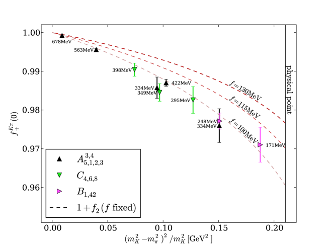
The ratios and in (9) from which we compute the form factor are constructed such that holds exactly even in a finite volume and for a finite lattice cut-off. We therefore expect finite-volume and cut-off effects to be symmetry-suppressed. Because of the automatic -improvement with domain wall Fermions on the coarse ensemble (B) we expect cut-off effects on the deviation of the form factor from one and on the finest ensemble (C) we expect these effects to be around 2%, where we have assumed MeV. A very good numerical confirmation that these effects are indeed below the statistical precision of our simulations can be seen in Figure 2. The plot provides a first impression of the simulation results plotted against ( should be linear in this variable for close to ). The data points for MeV (B42) and MeV (A, see pion mass labels in the plot) with fm and fm, respectively, lie on top of each other. Similarly, the MeV (A) and MeV (C6) simulation points for fm and fm, respectively, are in complete agreement and cut-off effects are therefore absent at the current level of precision.
The chiral effective theory for the quantities considered here predicts finite volume effects to be exponentially suppressed Ghorbani:2011gc ; Ghorbani:2013yh (proportional to ). The values of are summarised in Table 1 and they are all larger than 3.9. Finite volume effects are therefore expected to be of order 2% and below. Again, this uncertainty affects only the difference of the form factor from one which is a tiny effect. In this section we therefore assume that both lattice artifacts and finite-volume effects are below the statistical accuracy of the results. Further considerations will follow in the next section.
| id | fit ansatz for | d.o.f | ||
|---|---|---|---|---|
| 0.9584(16) | 0.6 | |||
| (15) | polynomial | 0.9565(17) | 0.7 | |
| (15) | polynomial | 0.9615(17) | 0.3 | |
| (15) | polynomial | 0.9639(18) | 0.4 | |
| (16) | polynomial | 0.9672(19) | 0.2 | |
| (17) | polynomial | 0.9670(20) | 0.2 | |
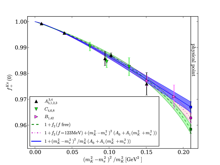
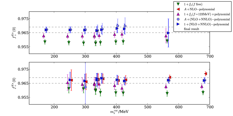
Figure 2 also shows the prediction of chiral perturbation theory at NLO for comparison, i.e. the expression , which depends strongly on the choice for the value of the decay constant used as input (shown for MeV). As already noted in Boyle:2010bh different choices for the value of the decay constant correspond to different forms for the NNLO-effects. In the full chiral expansion such effects are compensated by a change in the decay-constant’s contribution at higher order. Surprisingly, for a value of around MeV all the results seem to be reasonably well described by the NLO-ansatz without any NNLO corrections. We have therefore attempted to determine the decay constant from a fit to the data of only (fit ). The fits were of good quality (cf. the d.o.f.-values in Table 4). The functional form of fit is shown in Figure 3 (dashed central line and green error band) and Figure 4 illustrates how the fit result changes for different choices of the data points included (upside-down green triangles). The top panel shows how the results depend on variations of the lowest pion mass included into the fit (while including all heavier data points) and the bottom plot shows how the results change as the mass of the heaviest pion included into the fit is reduced (while including all results down to the lightest data point). While the central value of the form factor extrapolated to the physical point remained surprisingly stable given the simplicity of the fit function the results for the decay constant as a fit-parameter varied significantly between MeV and 101 MeV (not shown). As data points closer to the -symmetric limit are removed from the fit the central value moves a little towards larger values.
Given the wide range of simulated pion masses the performance of the ansatz is perhaps accidental and higher order terms in the chiral expansion play a role. The number of free parameters in the full NNLO-expression Bijnens:2003uy contained in is, however, too large to allow for a meaningful fit without further external constraints (cf. MILC Bazavov:2012cd who in their analysis of lattice data for the form factor constrain NNLO fits by using the low-energy constants from Bijnen’s “Fit 10” of chiral perturbation theory to experimental data Bijnens:2003uy ). In order to study potential higher order effects we employ a model Boyle:2007qe ; Boyle:2010bh ,
| (15) |
In addition to the dependence on the decay constant this expression has two further parameters, and . Allowing all three parameters to vary did not lead to stable fits – the final result showed a dependence on the choice of starting values for the -minimisation. We have therefore tried fits with the decay constant held fixed for a number of values in the range 95 MeV to 130 MeV (fits , and ). For a given choice of the results for are of good quality and stable under variation of the mass-cuts (cf. Figure 4 for 123 MeV). We did however find a monotonic variation of from 0.9565(17) to when increasing the value of from 95 MeV to 130 MeV (in each case fit to all ensembles). We have observed this behaviour previously in Boyle:2010bh where the final result for was determined from the fit of ansatz (15) to data set A with MeV and a systematic uncertainty due to the dependence on the decay constant was estimated from the variation of the central value between MeV and MeV. We note that the result GeV-4 and GeV-6 for fit agrees with what we found for the fit to data set A alone in Boyle:2010bh , GeV-4 and GeV-6.
As an alternative fit-form a naive polynomial parameterisation of the data seems equally appropriate, particularly as the lattice data further away from the -symmetric point shows little or no curvature. We therefore also consider the fit-ansätze (fit and ),
| (16) | |||||
| (17) |
These expressions are motivated by the expansion of (13) in . The parameter can either be set to 1, i.e. to the -symmetric limit or it can be left floating. The ansatz (16) leads to acceptable fit-quality only when the heavier data points are excluded (otherwise we found large values for d.o.f.). We have added the corresponding results only in the bottom panel of Figure 4. With the exception of the right-most point d.o.f.1, indicating that the linear ansatz describes the data well. Ansatz (17) with fixed to 1 leads to mutually compatible and good-quality fits over the full range of mass-cuts. Leaving freely floating has little impact on the fit results. We find for the fit over all data points which underlines the compatibility of our data with -symmetry and the absence of cut-off and finite volume effects in this limit to very high precision.
Fit and are very stable under a change of the mass-cut (cf. Figure 4, light blue circles and right-pointing blue triangles, respectively) with at the same time very small d.o.f.. We find the fit over all ensembles with ansatz (17) most convincing. The preferred fit-ansatz of our earlier study in Boyle:2010bh which was based on data set A only was (15). This ansatz is also compatible with the data and we use it in the following for an estimate of the model dependence.
6 Error budget and final results
In this section we estimate the magnitude of systematic uncertainties that need to be included in a comprehensive error budget. Following the discussion in Section 5 we estimate finite volume errors to be of order 2% and cutoff effects to be of order 5% on the difference of from 1. The simulation results indicate that these effects are indeed very small and below the level of statistical uncertainty. In order to remain conservative we attach a 5% error on for residual cutoff effects. We proceed in the same way for finite-size effects for which we attach a 2% error on . Uncertainties from the setting of the relative scale of the ensembles are reflected in the error on the lattice spacing which we have folded into the bootstrap analysis and are therefore included in the statistical error.
The chiral extrapolation for our final result is based on fit but ansatz (15) appears to be an adequate alternative with the caveat of the dependence on the external input . When varying the input in the fit with (15) the value of d.o.f. has a flat minimum around MeV. For this value of we find and we take the difference in central value between this fit result and fit as the residual model-dependence. After these considerations our final result is,
| (18) |
where in the last line we have added all systematic errors in quadrature. Our previous result Boyle:2010bh was based on data sets A with fit ansatz (15) where we were very cautious about the curvature suggested by the -term as one moves away from the -symmetric limit. We varied the value of the decay constant entering in order to quantify the induced systematic uncertainty. The result was . The central value is fully compatible with the same fit applied to the enlarged data set, fit .
The first applications of our result are predicting the CKM-matrix element and testing the unitarity of the CKM-matrix which is a crucial Standard Model test. In Antonelli:2010yf the experimental data for semileptonic decays was analysed. Their result combined with our result for gives
| (19) |
Together with the result Hardy:2008gy from super-allowed nuclear -decay and Beringer:1900zz we then confirm CKM-unitarity at the sub per mille level,
| (20) |
7 Discussion and Summary
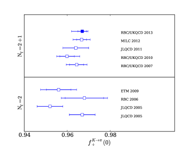
This work constitutes a comprehensive study of the kaon semileptonic decay form factor in three-flavour lattice QCD. Simulations in large lattice volumes with three values of the lattice spacing and pion masses in the range from as low as 171MeV up towards the -symmetric point allow for the detailed study of systematic effects. We have analysed the data using various ansätze for the remaining extrapolation to the physical point and we have identified a preferred functional form. After the extrapolation to the physical point we obtain the form factor with a statistical precision of 2 per mille and estimated per mille systematic errors. The prediction for the form factor, has an overall uncertainty of , where statistical and systematic uncertainties have been added in quadrature. Our collaboration is currently working on supplementing the data set by simulations performed directly at the physical point. These additional data will allow us to reduce the dominant systematic uncertainty, that due to the extrapolation in the quark mass to the physical point, very significantly. An overview of recent lattice results for the form factor including our new result is given in Figure 5.
An immediate phenomenological application of our result is the test of first-row CKM-matrix unitarity in the Standard Model which we are able to confirm at the sub per mille level.
Acknowledgements.
We are grateful to our colleagues within the RBC/UKQCD collaboration for sharing resources and gauge ensembles. The authors gratefully acknowledge computing time granted through the STFC funded DiRAC (Distributed Research utilising Advanced Computing) facility (grants ST/K005790/1, ST/K005804/1, ST/K000411/1, ST/H008845/1), through the Gauss Centre for Supercomputing (GCS) (via John von Neumann Institute for Computing (NIC)) on the GCS share of the supercomputers JUGENE/JUQUEEN at Jülich Supercomputing Centre (JSC) and the Engineering and Physical Sciences Research Council (EPSRC) for substantial allocation of time on HECToR under the Early User initiative and on the QCDOC supercomputer at the University of Edinburgh. AJ acknowledges funding from the European Research Council under the European Community’s Seventh Framework Programme (FP7/2007-2013) ERC grant agreement No 279757. JMF and CTS acknowledge support from STFC Grant ST/G000557/1 and EU contract MRTN-CT-2006-035482 (Flavianet). PAB and NG acknowledge support from STFC Grant ST/J000329/1 and KS is supported by the European Union under the Grant Agreement number 238353 (ITN STRONGnet). JMZ is supported by the Australian Research Council grant FT100100005.References
- (1) J. Hardy and I. Towner, Superallowed nuclear decays: A New survey with precision tests of the conserved vector current hypothesis and the standard model, Phys.Rev. C79 (2009) 055502, [arXiv:0812.1202].
- (2) M. Antonelli, V. Cirigliano, G. Isidori, F. Mescia, M. Moulson, et. al., An Evaluation of and precise tests of the Standard Model from world data on leptonic and semileptonic kaon decays, Eur.Phys.J. C69 (2010) 399–424, [arXiv:1005.2323].
- (3) G. Colangelo, S. Dürr, A. Jüttner, L. Lellouch, H. Leutwyler, et. al., Review of lattice results concerning low energy particle physics, Eur.Phys.J. C71 (2011) 1695, [arXiv:1011.4408].
- (4) S. Hashimoto, A. X. El-Khadra, A. S. Kronfeld, P. B. Mackenzie, S. M. Ryan, et. al., Lattice QCD calculation of anti- lepton anti-neutrino decay form-factors at zero recoil, Phys.Rev. D61 (1999) 014502, [hep-ph/9906376].
- (5) D. Becirevic et. al., The vector form factor at zero momentum transfer on the lattice, Nucl. Phys. B705 (2005) 339–362, [hep-ph/0403217].
- (6) P. A. Boyle, J. M. Flynn, A. Jüttner, C. T. Sachrajda, and J. M. Zanotti, Hadronic form factors in lattice QCD at small and vanishing momentum transfer, JHEP 05 (2007) 016, [hep-lat/0703005].
- (7) P. Boyle, J. Flynn, A. Jüttner, C. Kelly, C. Maynard, et. al., form factors with reduced model dependence, Eur.Phys.J. C69 (2010) 159–167, [arXiv:1004.0886].
- (8) ETM Collaboration Collaboration, V. Lubicz, F. Mescia, S. Simula, and C. Tarantino, for the ETM Collaboration, Semileptonic Form Factors from Two-Flavor Lattice QCD, Phys.Rev. D80 (2009) 111502, [arXiv:0906.4728].
- (9) P. A. Boyle et. al., semileptonic form factor from 2+1 flavour lattice QCD, Phys. Rev. Lett. 100 (2008) 141601, [0710.5136].
- (10) JLQCD Collaboration Collaboration, T. Kaneko et. al., Kaon semileptonic form factors in QCD with exact chiral symmetry, PoS LATTICE2011 (2011) 284, [arXiv:1112.5259].
- (11) A. Bazavov, C. Bernard, C. Bouchard, C. DeTar, D. Du, et. al., Kaon semileptonic vector form factor and determination of using staggered fermions, arXiv:1212.4993.
- (12) G. Amelino-Camelia, F. Archilli, D. Babusci, D. Badoni, G. Bencivenni, et. al., Physics with the KLOE-2 experiment at the upgraded DANE, Eur.Phys.J. C68 (2010) 619–681, [arXiv:1003.3868].
- (13) JLQCD Collaboration, N. Tsutsui et. al., Kaon semileptonic decay form factors in two-flavor QCD, PoS LAT2005 (2006) 357, [hep-lat/0510068].
- (14) C. Dawson, T. Izubuchi, T. Kaneko, S. Sasaki, and A. Soni, Vector form factor in semileptonic decay with two flavors of dynamical domain-wall quarks, Phys. Rev. D74 (2006) 114502, [hep-ph/0607162].
- (15) ETM Collaboration Collaboration, V. Lubicz, F. Mescia, L. Orifici, S. Simula, and C. Tarantino, Improved analysis of the scalar and vector form factors of kaon semileptonic decays with twisted-mass fermions, PoS LATTICE2010 (2010) 316, [arXiv:1012.3573].
- (16) RBC Collaboration, UKQCD Collaboration Collaboration, R. Arthur et. al., Domain Wall QCD with Near-Physical Pions, arXiv:1208.4412.
- (17) C. T. Sachrajda and G. Villadoro, Twisted boundary conditions in lattice simulations, Phys. Lett. B609 (2005) 73–85, [hep-lat/0411033].
- (18) P. F. Bedaque and J.-W. Chen, Twisted valence quarks and hadron interactions on the lattice, Phys. Lett. B616 (2005) 208–214, [hep-lat/0412023].
- (19) G. M. de Divitiis, R. Petronzio, and N. Tantalo, On the discretization of physical momenta in lattice QCD, Phys. Lett. B595 (2004) 408–413, [hep-lat/0405002].
- (20) UKQCD Collaboration, J. M. Flynn, A. Jüttner, and C. T. Sachrajda, A numerical study of partially twisted boundary conditions, Phys. Lett. B632 (2006) 313–318, [hep-lat/0506016].
- (21) Y. Iwasaki and T. Yoshie, Renormalization group improved action for lattice gauge theory and the string tension, Phys. Lett. B143 (1984) 449.
- (22) Y. Iwasaki, Renormalization Group Analysis of Lattice Theories and Improved Lattice Action: Two-Dimensional Nonlinear Sigma Model, Nucl. Phys. B258 (1985) 141–156.
- (23) D. B. Kaplan, A Method for simulating chiral fermions on the lattice, Phys. Lett. B288 (1992) 342–347, [hep-lat/9206013].
- (24) Y. Shamir, Chiral fermions from lattice boundaries, Nucl. Phys. B406 (1993) 90–106, [hep-lat/9303005].
- (25) RBC Collaboration, UKQCD Collaboration Collaboration, Y. Aoki et. al., Continuum Limit Physics from 2+1 Flavor Domain Wall QCD, Phys.Rev. D83 (2011) 074508, [arXiv:1011.0892].
- (26) RBC-UKQCD Collaboration, C. Allton et. al., Physical Results from 2+1 Flavor Domain Wall QCD and SU(2) Chiral Perturbation Theory, Phys. Rev. D78 (2008) 114509, [arXiv:0804.0473].
- (27) RBC and UKQCD Collaboration, C. Allton et. al., 2+1 flavor domain wall QCD on a lattice: light meson spectroscopy with , Phys. Rev. D76 (2007) 014504, [hep-lat/0701013].
- (28) Y. Aoki, R. Arthur, T. Blum, P. Boyle, D. Brommel, et. al., Continuum Limit of from 2+1 Flavor Domain Wall QCD, Phys.Rev. D84 (2011) 014503, [arXiv:1012.4178].
- (29) B. Efron, Bootstrap methods: another look at the jacknife, Ann. Statist. 7 (1979) 1–26.
- (30) UKQCD Collaboration Collaboration, M. Foster and C. Michael, Quark mass dependence of hadron masses from lattice QCD, Phys.Rev. D59 (1999) 074503, [hep-lat/9810021].
- (31) UKQCD Collaboration Collaboration, C. McNeile and C. Michael, Decay width of light quark hybrid meson from the lattice, Phys.Rev. D73 (2006) 074506, [hep-lat/0603007].
- (32) P. Boyle, A. Jüttner, C. Kelly, and R. Kenway, Use of stochastic sources for the lattice determination of light quark physics, JHEP 0808 (2008) 086, [arXiv:0804.1501].
- (33) Particle Data Group Collaboration, J. Beringer et. al., Review of Particle Physics (RPP), Phys.Rev. D86 (2012) 010001.
- (34) J. Gasser and H. Leutwyler, Low-Energy Expansion of Meson Form-Factors, Nucl. Phys. B250 (1985) 517–538.
- (35) M. Ademollo and R. Gatto, Nonrenormalization Theorem for the Strangeness Violating Vector Currents, Phys.Rev.Lett. 13 (1964) 264–265.
- (36) J. Bijnens and P. Talavera, K(l3) decays in chiral perturbation theory, Nucl. Phys. B669 (2003) 341–362, [hep-ph/0303103].
- (37) K. Ghorbani, Chiral and Volume Extrapolation of Pion and Kaon Electromagnetic form Factor within SU(3) ChPT, arXiv:1112.0729.
- (38) K. Ghorbani, Kaon semi-leptonic form factor at zero momentum transfer in finite volume, arXiv:1301.0919.