Rutgers relation for the analysis of superfluid density in superconductors

Abstract

It is shown that the thermodynamic Rutgers relation for the second order phase transitions can be used for the analysis of the superfluid density data irrespective of complexities of the Fermi surface, structure of the superconducting gap, pairing strength, or scattering. The only limitation is that critical fluctuations should be weak, so that the mean field theory of the second order phase transitions is applicable. By using the Rutgers relation, the zero temperature value of the London penetration depth, $\lambda(0)$, is related to the specific heat jump $\Delta C$ and the slope of upper critical field $dH_{c2}/dT$ at the transition temperature $T_{c}$, provided the data on $\Delta\lambda=\lambda(T)-\lambda(0)$ are available in a broad temperature domain. We then provide a new way of determination of $\lambda(0)$, the quantity difficult to determine within many techniques.

I Introduction

The London penetration depth $\lambda$ is one of the most important characteristic length scales of superconductors. The temperature dependent $\lambda(T)$ is subject of many studies, as it provides information on the symmetry of the order parameter.Prozorov and Giannetta (2006); Prozorov and Kogan (2011) It is used to calculate the superfluid density, $\rho(T)\equiv\lambda^{2}(0)/\lambda^{2}(T)$, a quantity that can be directly compared with theory. Determination of $\lambda(0)$ is critical because the shape of $\rho(T)$ extracted from the data on $\Delta\lambda(T)$ depends sensitively on the value of $\lambda(0)$ adopted, and a wrong $\lambda(0)$ could lead to incorrect conclusions on the superconducting order parameter.

Tunnel diode resonator (TDR) provides perhaps the most precise measurements of the variation of $\lambda$ with temperature, $\Delta\lambda=\lambda(T)-\lambda(0)$. With additional sample manipulation by coating it with lower-$T_{c}$ superconductor, the absolute value of $\lambda(0)$ can be determined as well, but with much lower precision compared to $\Delta\lambda$.Prozorov et al. (2000) Other techniques which are used to measure $\lambda(0)$ include muon spin rotation ($\mu$SR),Sonier (2007) infrared spectroscopy,Basov and Timusk (2005) and microwave cavity perturbation technique,Kamal et al. (1998) and local probes.Lippman et al. (2012); Luan et al. (2010) However, each of these techniques has its own limitations. $\mu$SR measures averaged $\lambda(T,H)$ in the mixed state and extrapolated to $H=0$ value is used to estimate $\lambda(0)$. In infrared spectroscopy, $\lambda(0)$ is deduced from the measured plasma frequency, which is not a precisely determined quantity.Basov and Timusk (2005) Local probes, such as scanning SQUID Lippman et al. (2012) and MFM Luan et al. (2010) magnetometry, infer $\lambda(0)$ from the analysis of magnetic interactions between a relevant probe and a magnetic moment induced in a superconductor.Kirtley (2010)

In this paper we show that the thermodynamic relation between the specific heat jump, $\Delta C$, and the slope of thermodynamic critical field, $\partial H_{c}/\partial T$, at the superconducting transition temperature, $T_{c}$, first proposed by Rutgers Rutgers (1934), can be rewritten in terms of measurable quantities, - the slopes of the upper critical field and of the superfluid density in addition to specific heat jump. As a general thermodynamic relation valid at the 2nd order transition (excluding critical fluctuation region), it is applicable for any superconductor irrespective of the pairing symmetry, scattering or multiband nature of superconductivity, as we verified on several well-known systems. Such general applicability of the Rutgers relation offers a method of estimating $\lambda(0)$ if $\Delta C$ and $dH_{c2}/dT$ at $T_{c}$ are known. This idea is checked on Nb and MgB₂ and applied to several unconventional superconductors. In all cases we use $\Delta\lambda(T)$ measured by the TDR technique and the literature data for the other two quantities except for YBa₂Cu₃O_1-δ where its $\rho(T)$ was taken from Ref.Kamal et al., 1998. In all studied cases, the method works well and determined values of $\lambda(0)$ are in agreement with the literature.

I.1 Thermodynamic Rutgers relation

The specific heat jump at $T_{c}$ in materials where the critical fluctuations are weak is expressed through the free energy difference $F_{n}-F_{s}=H_{c}^{2}/8\pi$:Rutgers (1934); Lifshitz et al. (1984)

$$\Delta C=T_{c}\frac{\partial^{2}}{\partial T^{2}}\frac{H_{c}^{2}}{8\pi}\Big{|}_{T_{c}}=\frac{T_{c}}{4\pi}\left(\frac{\partial H_{c}}{\partial T}\right)^{2}_{T_{c}}$$ (1)

Here, $C$ is measured in erg/cm³K and $T$ in K. Within the mean-field Ginzburg-Landau (GL) theory, near $T_{c}$, the thermodynamic critical field $H_{c}=\phi_{0}/2\sqrt{2}\pi\xi\lambda$ with

$$(\xi,\lambda)=\frac{(\xi_{GL},\lambda_{GL})}{\sqrt{1-t}}\,,\qquad t=\frac{T}{T_{c}}\,.$$ (2)

Here $\xi$ and $\lambda$ are the coherence length and the penetration depth, and the constants $\xi_{GL},\lambda_{GL}$ are of the same order but not the same as the zero$-T$ values $\xi(0)$ and $\lambda(0)$. Hence we have:

$$\Delta C=\frac{\phi_{0}^{2}}{32\pi^{3}\xi_{GL}^{2}\lambda_{GL}^{2}T_{c}}\,,$$ (3)

where $\xi_{GL}$ is related to the slope of $H_{c2}(T)$ at $T_{c}$:

$$T_{c}\frac{\partial H_{c2}}{\partial T}\Big{|}_{T_{c}}=\frac{\partial H_{c2}}{\partial t}\Big{|}_{t=1}=-\frac{\phi_{0}}{2\pi\xi_{GL}^{2}}\,.$$ (4)

It is common to introduce the dimensionless superfluid density $\rho=\lambda^{2}(0)/\lambda^{2}$ with the slope at $T_{c}$ given by

$$T_{c}\frac{\partial\rho}{\partial T}\Big{|}_{T_{c}}=\frac{\partial\rho}{\partial t}\Big{|}_{t=1}=-\frac{\lambda^{2}(0)}{\lambda_{GL}^{2}}\,.$$ (5)

We then obtain:

$$\Delta C=\frac{\phi_{0}}{16\pi^{2}\lambda^{2}(0)T_{c}}\,\left(H_{c2}^{\prime}\,\rho^{\prime}\right)_{t=1}$$ (6)

where the primes denote derivatives with respect to $t$.

It should be stressed that being a thermodynamic relation that holds at a 2nd order phase transition, applicability of Rutgers formula is restricted only by possible presence of critical fluctuations. In particular, it can be applied for zero-field phase transition in materials with anisotropic order parameters and Fermi surfaces, multi-band etc, which makes it a valuable tool in studying great majority of new materials.

For anisotropic materials, Eq. (1) is, of course, valid since the condensation energy and $H_{c}$ do not depend on direction. However, already in Eq. (3) the field direction should be specified. In the following we discuss situations with ${\bm{H}}$ parallel to the $c$ axis of uniaxial crystals. Hence, $H_{c2},\rho$, and $\lambda(0)$ in Eq. (6) should have subscripts $ab$; we omit them for brevity. A general case of anisotropic material with arbitrary field orientation requires separate analysis.

II Determination of $\lambda(0)$

The full superfluid density needed for the analysis of the experimental data and comparison with theoretical calculations depends on the choice of $\lambda(0)$:

$$\rho(t)=\frac{\lambda^{2}(0)}{[\lambda(0)+\Delta\lambda(t)]^{2}}\,.$$ (7)

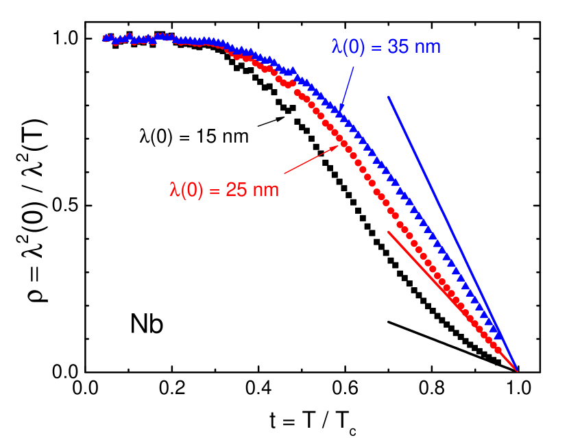
Figure 1: (Color online) Superfluid density $\rho(t)$ calculated from Eq. (7) using the TDR data on $\Delta\lambda(T)$ and assuming $\lambda(0)=$ 15, 25, and 35 nm. Straight lines have the slope $\rho^{\prime}$ estimated from Eq. (6) for each $\lambda(0)$.

Figure 1 shows an example of this dependence of $\rho(t)$ on $\lambda(0)$ for Nb. Symbols represent $\rho(t)$ calculated from measured $\Delta\lambda(t)$ with $\lambda(0)$ chosen as 15, 25 and 35 nm. Clearly, the calculated $\rho(t)$ is sensitive to the choice of $\lambda(0)$. The straight solid lines have the slope $\rho^{\prime}(1)$ calculated by using Eq. (6) for each $\lambda(0)$. We used $\Delta C=137.2$ mJ/mol-K $=126450$ erg/cm³K (Ref. Weber et al., 1991) since in the formulas used here the specific heat is per unit volume. Using $H_{c2}^{\prime}|_{T_{c}}=440$ Oe/K (Ref. Williamson, 1970), we obtain $-\rho^{\prime}(1)=$ 0.49, 1.4, and 2.7 for 15, 25, and 35 nm, respectively. While the choice of $\lambda(0)=25$ nm shows reasonable agreement, for the choices of 15 nm and 35 nm the slopes calculated using the data and Eq. (7) determined by Eq. (6) under- and over-estimates, respectively. Note that with $\lambda(0)=15$ nm, the temperature dependence of $\rho$ is pronouncedly concave near $t=1$, and also $-\rho^{\prime}(1)$ is smaller than one. The idea of our method is to utilize the Rutgers relation (6) and choose such a $\lambda(0)$ that would not contradict the thermodynamics near $T_{c}$.

To this end we rewrite Eq. (6) in the form:

$$\frac{\rho^{\prime}(1)}{\lambda^{2}(0)}=\frac{16\pi^{2}T_{c}\Delta C}{\phi_{0}H^{\prime}_{c2}(1)}\,.$$ (8)

The right-hand side here is determined from independent measurements of $\Delta C$ and $H_{c2}$. Thus, by taking a few test values of $\lambda(0)$, calculating $\rho(t)$ and its slope at $t=1$, we can decide which $\lambda(0)$ and $\rho(t,\lambda(0))$ obey the Rutgers relation.

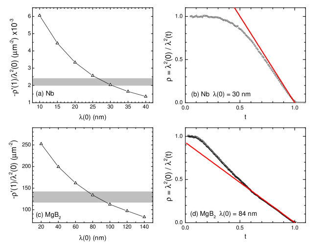
Figure 2: Top row - Nb, Bottom row - MgB₂. Left column: variation of $|\rho^{\prime}|/\lambda^{2}(0)$ as a function of $\lambda(0)$ for Nb and MgB₂. Shaded horizontal bands are the estimated values of the right-hand side of Eq. (8) with literature values of $\Delta C$ and $H_{c2}^{\prime}(1)$ including experimental uncertainties. Right column: superfluid density for the best value of $\lambda(0)$ that satisfies the Rutgers relation, Eq. (8).

We first apply this method to two well-studied superconductors - conventional Nb and two-band MgB₂. For Nb, we obtain $|\rho^{\prime}|/\lambda^{2}(0)\approx 2240$ $\mu$m^-2 using the same thermodynamic quantities as for Fig. 1. Weber et al. (1991); Williamson (1970) We now take a set of values for $\lambda(0)$ shown in top left panel of Fig. 2 and plot $|\rho^{\prime}|/\lambda^{2}(0)$ vs $\lambda(0)$. The value of $\lambda(0)=28\pm 2\,$nm satisfying the Rutgers relation is obtained from the intersection of the calculated curve with the value expected from Eq. (8) (shown by a gray band that takes into account experimental uncertainties in determining $\Delta C$ and $H^{\prime}_{c2}$). It is consistent with the literature values varying between 26 and 39 nm.Weber et al. (1991); Maxfield and McLean (1965) The final calculated superfluid density with the choice of $\lambda(0)=30$ nm is shown in Fig. 2(b). The solid line is determined with the calculated slope $|\rho^{\prime}(1)|=2$, as predicted for isotropic s-wave superconductors (see, Appendix).

In addition to the aforementioned uncertainties, determination of the experimental $|\rho^{\prime}(1)|$ is not trivial even if the quality of measurement is excellent since $\rho(t)$ near $t=1$ is often significantly curved due to several experimental artifacts, most importantly due to the influence of the normal skin effect near $T_{c}$, which is more pronounced for higher frequency measurements on highly conducting materials. TDR technique uses typically $\sim 10$ MHz, so this effect is weak in most of the materials concerned. Analyzing the data for different superconductors, we have found that the data in the regime between $t=0.8$ and 0.95 works well for the determination of $\rho^{\prime}(1)$. The experimental $|\rho^{\prime}(1)|$ in this work is determined from the best linear fit of $\rho(t)$ data in this range.

The same procedure can be employed for a well known multi gap superconductor MgB₂ (shown in the bottom row of Fig. 2), where $|\rho^{\prime}|/\lambda^{2}(0)$ is estimated to be $130\pm 12$ $\mu$m^-2 by using $\Delta C=133$ mJ/mol-K (Ref. Bouquet et al., 2001), $|H^{\prime}_{c2}(1)|=0.45$ T/K (Ref. Bud’ko et al., 2001) within $\pm$5% error. The determined $\lambda(0)=84\pm 10\,$nm is in good agreement with 100 nm estimated by $\mu$SR technique.Niedermayer et al. (2002); Ohishi et al. (2003) For $\lambda(0)=84$ nm, the calculated slope $|\rho^{\prime}(1)|=0.91$ agrees with the expected theoretical value of 0.92. (appendix).

The method described has also been used for SrPd₂Ge₂ for which $\lambda(0)$ was not clear. By using the determined $\lambda(0)$ we have shown that SrPd₂Ge₂ is a single-gap s-wave superconductor.Kim et al. (2013)

II.1 Unconventional superconductors

Table 1: $V_{c}$ is the volume of the unit cell. $\Delta C$ is the specific heat jump at $T_{c}$ in mJ/mol-K. $dH_{c2}/dT$ is slope of $H_{c2}$ at $T_{c}$. $\rho^{\prime}_{Rut}=(d\rho/dt)_{Rut}$ is the calculated slope using Eq. (6) where $t=T/T_{c}$. $\rho^{\prime}_{exp}$ is an experimental slope with given $\lambda(0)$.

compound	$V_{c}$  (Å3)	$T_{c}$ (K)	$\Delta C/T_{c}$ (mJ/mol-K2)	$|dH_{c2}/dT|_{T_{c}}$ (T/K)	$\lambda(0)$ (nm)	$-\rho^{\prime}_{Rut}$	$-\rho^{\prime}_{exp}$
Nb	35.937 [Ito et al., 2006]	9.3 [Weber et al., 1991]	14.8 [Weber et al., 1991]	0.044 [Williamson, 1970]	30	2.0	1.8
MgB2	$29.064$ [Nagamatsu et al., 2001]	39 [Bouquet et al., 2001]	3.4 [Bouquet et al., 2001]	$0.45$ [Bud’ko et al., 2001]	84	0.91	$0.83$
LiFeAs	$90.252$ [Tapp et al., 2008]	15.4 [Wei et al., 2010]	20 [Wei et al., 2010]	3.46 [Cho et al., 2011]	200 [Pratt et al., 2009]	1.2	1.1
FeTe0.58Se0.42	87.084 [Johnston, 2010]	14 [Braithwaite et al., 2010]	20 [Braithwaite et al., 2010]	13 [Klein et al., 2010]	500	1.4	1.5
YBa2Cu3O1-δ	173.57 [Poole et al., 2010]	23 [Kim et al., 2012]	61 [Wang et al., 2001]	1.9 [Welp et al., 1989]	120 [Prozorov et al., 2000]	3.0	2.15 - 4.98 [Kamal et al., 1998]
MgCNi3	54.496 [Shan et al., 2003]	7 [Shan et al., 2003]	129 [Shan et al., 2003]	2.6 [Poole et al., 2010]	232 [MacDougall et al., 2006]	1.8	2.0

Here we examine the validity of our approach for some superconductors for which the necessary experimental quantities have been reported in the literature. Where possible, we use $H_{c2}(T)$ determined from the specific heat jump, because resistive and magnetic measurements may actually determine the irreversibility field, which may differ substantially from the thermodynamic $H_{c2}$.Carrington et al. (1996)

We have selected LiFeAs, FeTe_0.58Se_0.42, YBa₂Cu₃O_1-δ and MgCNi₃ representing stoichiometric pnictide, charchogenide, d-wave high-$T_{c}$ cuprate and close to magnetic instability s-wave superconductor, respectively. $\Delta C$, $dH_{c2}/dT$, and $\lambda(0)$ for the selected compounds have been measured by various techniques by different groups. The superfluid density was calculated from the penetration depth measured by using a TDR technique at Ames Laboratory, except for YBCO for which anisotropic superfluid density was determined by microwave cavity perturbation technique.Kamal et al. (1998) Thermodynamic parameters are discussed in the number of papers.Johnston (2010); Canfield and Bud’ko (2010); Stewart (2011) In-depth discussion of the specific heat is given in Refs. Stewart, 2011; Kim et al., 2012. Table 1 summarizes parameters used in the calculations.

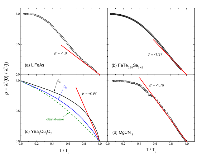
Figure 3: Experimental superfluid density $\rho=\lambda^{2}(0)/\lambda^{2}(T)$ in LiFeAs, FeTe_0.58Se_0.42, YBa₂Cu₃O_1-δ, and MgCNi₃ with $\lambda(0)=$ 500, 200, 120, and 232 nm, respectively. The straight lines in each panel were estimated with the Rutgers formula. Parameters used for the calculation are summarized in Table 1.

Figure 3 shows experimental superfluid density in LiFeAs, FeTe_0.58Se_0.42, YBa₂Cu₃O_1-δ and MgCNi₃ with $\lambda(0)=500$, 200, 120, and 232 nm, respectively. The agreement between $\rho^{\prime}_{Rut}$ calculated with the Rutgers relation and $\rho^{\prime}_{exp}$ extracted from the data on $\Delta\lambda(t)$, given possible uncertainties in the input experimental parameters, is rather remarkable.

III Summary

In conclusion, we have shown that the thermodynamic relation based on Rutgers formula can be used for the analysis of the superfluid density. Based on this relation, a method to estimate $\lambda(0)$ is developed. As a test, it was successfully applied to reproduce known $\lambda(0)$ in Nb and MgB₂. We used this relation to verify reported literature values of $\lambda(0)$ for several unconventional superconductors of different band structure, gap anisotropy, and pairing symmetry.

IV ACKNOWLEDGMENTS

We thank A. Chubukov for useful discussions. The work was supported by the U.S. Department of Energy, Office of Basic Energy Sciences, Division of Materials Sciences and Engineering under contract No. DE-AC02-07CH11358.

Appendix A Theoretical results relevant for the analysis of the superfluid density

A.1 Penetration depth in anisotropic materials

It is knownFetter and Hohenberg (1969) that in isotropic materials,

$$\rho^{\prime}(1)=\lambda^{2}(0)/\lambda_{GL}^{2}=-2\,.$$ (9)

It is easy to reproduce this result for the free electron model of the normal state; it is shown below, however, that this value holds for any Fermi surface provided the order parameter is isotropic.

Here, we are interested in relating $\lambda(0)$ and $\lambda_{GL}$, the $T$ independent part of $\lambda$ near $T_{c}$, for anisotropic Fermi surfaces and order parameters. We start with a known relation,

$$(\lambda^{2})_{ik}^{-1}=\frac{16\pi^{2}e^{2}N(0)T}{c^{2}}\sum_{\omega}\left\langle\frac{\Delta^{2}v_{i}v_{k}}{\beta^{3}}\right\rangle\,,$$ (10)

which holds at any temperature for clean materials with arbitrary Fermi surface and order parameter anisotropies.Kogan (2002); Prozorov and Kogan (2011) Here, $N(0)$ is the density of states at the Fermi level per spin, $\beta^{2}=\Delta^{2}+\hbar^{2}\omega^{2}$ with $\hbar\omega=\pi T(2n+1)$, $\Delta({\bm{k}}_{F},T)=\Psi(T)\Omega({\bm{k}}_{F})$ is the zero-field order parameter which in general depends on the position ${\bm{k}}_{F}$ on the Fermi surface, and $\langle...\rangle$ stand for averaging over the Fermi surface. The function $\Omega({\bm{k}}_{F})$ which describes the variation of $\Delta$ along the Fermi surface, is normalized: $\left\langle\Omega^{2}\right\rangle=1$.

Eq. (10) is obtained within the model of factorizable effective coupling $V({\bm{k}},{\bm{k}}^{\prime})=V_{0}\,\Omega({\bm{k}})\,\Omega({\bm{k}}^{\prime})$.Markowitz and Kadanoff (1963) The self-consistency equation of the weak coupling theory takes the form:

$$\Psi({\bm{r}},T)=2\pi TN(0)V_{0}\sum_{\omega>0}^{\omega_{D}}\Big{\langle}\Omega({\bm{k}})f({\bm{k}},{\bm{r}},\omega)\Big{\rangle}\,,$$ (11)

where $f$ is the Eilenberger Green’s function which, for the uniform current-free state, reads: $f=\Delta/\beta=\Psi\Omega/\beta$. The order parameter near $T_{c}$ is now readily obtained:

$$\Psi^{2}=\frac{8\pi^{2}T_{c}^{2}(1-t)}{7\zeta(3)\langle\Omega^{4}\rangle}\,,$$ (12)

which reduces to the isotropic BCS form for $\Omega=1$. We substitute this in Eq. (10) to obtain near $T_{c}$:

$$(\lambda^{2})_{ik}^{-1}=\frac{16\pi e^{2}N(0)\langle\Omega^{2}v_{i}v_{k}\rangle}{c^{2}\langle\Omega^{4}\rangle}\,(1-t)\,,$$ (13)

from which the constants $\lambda_{GL}$ for any direction readily follow.

As $T\to 0$, the sum over the Matsubara frequencies in Eq. (10) can be replaced with an integral according to $2\pi T\sum_{\omega}\to\int_{0}^{\infty}d(\hbar\omega)$:

$$(\lambda^{2})_{ik}^{-1}(0)=\frac{8\pi e^{2}N(0)}{c^{2}}\,\Big{\langle}v_{i}v_{k}\Big{\rangle}\,.$$ (14)

For free electrons, this reduces to the London value $\lambda^{2}=mc^{2}/4\pi e^{2}n$ where $n=2mN(0)v^{2}/3$ is the electron density.

Hence, we get for the slope of the in-plane superfluid density:

$$\rho_{ab}^{\prime}(1)=-\frac{\lambda^{2}_{ab}(0)}{\lambda^{2}_{GL,ab}}=-2\frac{\langle\Omega^{2}v^{2}_{a}\rangle}{\langle v_{a}^{2}\rangle\langle\Omega^{4}\rangle}\,.$$ (15)

Similarly, one can define $\rho_{c}^{\prime}(1)$ for which $v_{a}$ should be replaced with $v_{c}$ in Eq. (15). In particular, we have:

$$\frac{\rho_{c}^{\prime}(1)}{\rho_{ab}^{\prime}(1)}=\frac{\langle v^{2}_{a}\rangle}{\langle v_{c}^{2}\rangle}\,\frac{\langle\Omega^{2}v^{2}_{c}\rangle}{\langle\Omega^{2}v^{2}_{a}\rangle}=\frac{\gamma_{\lambda}^{2}(0)}{\gamma_{\lambda}^{2}(T_{c})}\,.$$ (16)

E.g., for MgB₂ with $\gamma_{\lambda}(0)\approx 1$, $\gamma_{\lambda}(T_{c})\approx 2.6$, we estimate $\rho_{c}^{\prime}(1)\approx 0.15\,\rho_{ab}^{\prime}(1)$.

It is instructive to note that $\rho^{\prime}(1)$ reduces to the isotropic value of $-2$ for any Fermi surface provided the order parameter is constant, $\Omega=1$.

A.2 MgB₂

Consider a simple two-band model with the gap anisotropy given by

$$\Omega({\textbf{k}})=\Omega_{1,2}\,,\quad{\textbf{k}}\in F_{1,2}\,,$$ (17)

where $F_{1},F_{2}$ are two sheets of the Fermi surface. $\Omega_{1,2}$ are assumed constants, in other words, we model MgB₂ as having two different s-wave gaps. The normalization $\langle\Omega^{2}\rangle=1$ then gives:

$$\Omega_{1}^{2}\nu_{1}+\Omega_{2}^{2}\nu_{2}=1\,,\quad\nu_{1}+\nu_{2}=1\,,$$ (18)

where $\nu_{1,2}=N_{1,2}/N(0)$ are the relative densities of states.

Based on the band structure calculations,Belashchenko et al. (2001); Choi et al. (2002) $\nu_{1}$ and $\nu_{2}$ of our model are $\approx\,$0.56 and 0.44. The ratio $\Delta_{2}/\Delta_{1}=\Omega_{2}/\Omega_{1}\approx 3$. Then, the normalization (18) yields $\Omega_{1}=0.47$ and $\Omega_{2}=1.41$.

Further, we use the averages over separate Fermi sheets calculated in Ref. Belashchenko et al., 2001: $\langle v_{a}^{2}\rangle_{1}=33.2$, $\langle v_{a}^{2}\rangle_{2}=23$ cm²/s². With this input, we estimate

$$\rho_{ab}^{\prime}(1)=-0.92\,.$$ (19)

It should be noted that this number is sensitive to a number of input parameters. The procedure described above, see Fig. 2, gives $\rho_{ab}^{\prime}(1)\approx-0.91$.

Since only even powers of $\Omega$ enter Eq. (15), the same analysis of the slope $\rho^{\prime}(1)$ can, in fact, be exercised for materials modeled by two bands with the $\pm s$ symmetry of the order parameter, for which $\Omega$’s have opposite signs. If the bands relative densities of state $\nu_{1,2}$ and the averages $\langle v_{a}^{2}\rangle_{1,2}$ are comparable to each other and similar to those of MgB₂, we expect a similar $|\rho^{\prime}(1)|\approx 1$ for clean crystals.

A.3 d-wave

It can be shown that $\Omega=\sqrt{2}\cos 2\phi$ for closed Fermi surfaces as rotational ellipsoids (in particular, spheres) or open ones as rotational hyperboloids (in particular, cylinders).Kogan and Prozorov (2012) A straightforward algebra gives:

$$\rho^{\prime}_{ab}(1)=-4/3\,.$$ (20)

A.4 Scattering

In the limit of a strong non-magnetic scattering for an arbitrary Fermi surface but a constant s-wave order parameter we have, see, e.g, Ref. Prozorov and Kogan, 2011:

$$(\lambda^{2})_{ik}^{-1}=\frac{8\pi^{2}e^{2}N(0)\langle v_{i}v_{k}\rangle\tau}{c^{2}\hbar}\,\Delta\tanh\frac{\Delta}{2T}\,.$$ (21)

Here $\tau$ is the average scattering time. It is worth noting that the dirty limit does not make much sense for anisotropic gaps because $T_{c}$ is suppressed even by non-magnetic scattering in the limit $\tau\to 0$. At $T=0$, we have

$$(\lambda^{2})_{ik}^{-1}(0)=\frac{8\pi^{2}e^{2}N(0)\langle v_{i}v_{k}\rangle\tau}{c^{2}\hbar}\,\Delta(0)\,,$$ (22)

whereas near $T_{c}$

$$(\lambda^{2})_{ik}^{-1}=\frac{8\pi^{2}e^{2}N(0)\langle v_{i}v_{k}\rangle\tau}{c^{2}\hbar}\,\frac{\Delta^{2}}{2T_{c}}\,,$$ (23)

Since for non-magnetic scattering, $T_{c}$ and $\Delta(T)$ are the same as in the clean case, in particular $\Delta=8\pi^{2}T_{c}^{2}(1-t)/7\zeta(3)$, we obtain

$$\rho^{\prime}(1)=-\frac{4\pi^{2}T_{c}}{\Delta(0)}=-\frac{4\pi e^{\gamma}}{7\zeta(3)}=-2.66\,.$$ (24)

We thus conclude that scattering causes the slope $\rho^{\prime}(1)$ to increase.

Evaluation of scattering effects on the slope $\rho^{\prime}$ near $T_{c}$ for anisotropic gaps and Fermi surfaces are more involved because both $T_{c}$ and $\Delta$ are affected even by non-magnetic scattering. The case of a strong pair-breaking is an exception: $\lambda^{-2}=\lambda^{-2}_{0}(1-t^{2})$ that immediately gives $\rho^{\prime}(1)=-2$.

References

- Prozorov and Giannetta (2006) R. Prozorov and R. W. Giannetta, Superconductor Science and Technology 19, R41 (2006).
- Prozorov and Kogan (2011) R. Prozorov and V. G. Kogan, Rep. Prog. Phys. 74, 124505 (2011).
- Prozorov et al. (2000) R. Prozorov, R. W. Giannetta, A. Carrington, P. Fournier, R. L. Greene, P. Guptasarma, D. G. Hinks, and A. R. Banks, Appl. Phys. Lett. 77, 4202 (2000).
- Sonier (2007) J. E. Sonier, Rep. Prog. Phys. 70, 1717 (2007).
- Basov and Timusk (2005) D. N. Basov and T. Timusk, Rev. Mod. Phys. 77, 721 (2005).
- Kamal et al. (1998) S. Kamal, R. Liang, A. Hosseini, D. A. Bonn, and W. N. Hardy, Phys. Rev. B 58, R8933 (1998).
- Lippman et al. (2012) T. M. Lippman, B. Kalisky, H. Kim, M. A. Tanatar, S. L. Bud‰Ûªko, P. C. Canfield, R. Prozorov, and K. A. Moler, Physica C: Superconductivity 483, 91 (2012).
- Luan et al. (2010) L. Luan, O. M. Auslaender, T. M. Lippman, C. W. Hicks, B. Kalisky, J.-H. Chu, J. G. Analytis, I. R. Fisher, J. R. Kirtley, and K. A. Moler, Phys. Rev. B 81, 100501 (2010).
- Kirtley (2010) J. R. Kirtley, Reports on Progress in Physics 73, 126501 (2010).
- Rutgers (1934) A. Rutgers, Physica 1, 1055 (1934).
- Lifshitz et al. (1984) E. M. Lifshitz, L. D. Landau, and L. P. Pitaevskii, Electrodynamics of Continuous Media, 2nd ed. (Butterworth-Heinemann, 1984).
- Weber et al. (1991) H. W. Weber, E. Seidl, C. Laa, E. Schachinger, M. Prohammer, A. Junod, and D. Eckert, Phys. Rev. B 44, 7585 (1991).
- Note (1) To convert which is commonly reported in mJ/mol-K into erg/cm3K, one needs to calculate the mass density which requires crystallographic information. For niobium we use parameters found in Ref. \rev@citealpnumIto2006. Crystal structure of elemental niobium belongs to the space group Im-3m (no. 229) with lattice parameters nm, and corresponding volume is nm3. There are two molecular units per the volume (). Using these values the converted mJ/mol-K (Ref. \rev@citealpnumWeber1991) erg/cm3K.
- Williamson (1970) S. J. Williamson, Phys. Rev. B 2, 3545 (1970).
- Maxfield and McLean (1965) B. W. Maxfield and W. L. McLean, Phys. Rev. 139, A1515 (1965).
- Bouquet et al. (2001) F. Bouquet, R. A. Fisher, N. E. Phillips, D. G. Hinks, and J. D. Jorgensen, Phys. Rev. Lett. 87, 047001 (2001).
- Bud’ko et al. (2001) S. L. Bud’ko, C. Petrovic, G. Lapertot, C. E. Cunningham, P. C. Canfield, M.-H. Jung, and A. H. Lacerda, Phys. Rev. B 63, 220503 (2001).
- Niedermayer et al. (2002) C. Niedermayer, C. Bernhard, T. Holden, R. K. Kremer, and K. Ahn, Phys. Rev. B 65, 094512 (2002).
- Ohishi et al. (2003) K. Ohishi, T. Muranaka, J. Akimitsu, A. Koda, W. Higemoto, and R. Kadono, J. Phys. Soc. Japan 72, 29 (2003).
- Kim et al. (2013) H. Kim, N. H. Sung, B. K. Cho, M. A. Tanatar, and R. Prozorov, Phys. Rev. B 87, 094515 (2013).
- Ito et al. (2006) M. Ito, H. Muta, M. Uno, and S. Yamanaka, J. Alloys and Comp. 425, 164 (2006).
- Nagamatsu et al. (2001) J. Nagamatsu, N. Nakagawa, T. Muranaka, Y. Zenitani, and J. Akimitsu, Nature 410, 63 (2001).
- Tapp et al. (2008) J. H. Tapp, Z. Tang, B. Lv, K. Sasmal, B. Lorenz, P. C. W. Chu, and A. M. Guloy, Phys. Rev. B 78, 060505 (2008).
- Wei et al. (2010) F. Wei, F. Chen, K. Sasmal, B. Lv, Z. J. Tang, Y. Y. Xue, A. M. Guloy, and C. W. Chu, Phys. Rev. B 81, 134527 (2010).
- Cho et al. (2011) K. Cho, H. Kim, M. A. Tanatar, Y. J. Song, Y. S. Kwon, W. A. Coniglio, C. C. Agosta, A. Gurevich, and R. Prozorov, Phys. Rev. B 83, 060502 (2011).
- Pratt et al. (2009) F. L. Pratt, P. J. Baker, S. J. Blundell, T. Lancaster, H. J. Lewtas, P. Adamson, M. J. Pitcher, D. R. Parker, and S. J. Clarke, Phys. Rev. B 79, 052508 (2009).
- Johnston (2010) D. C. Johnston, Adv. Phys. 59, 803 (2010).
- Braithwaite et al. (2010) D. Braithwaite, G. Lapertot, W. Knafo, and I. Sheikin, Journal of the Physical Society of Japan 79, 053703 (2010).
- Klein et al. (2010) T. Klein, D. Braithwaite, A. Demuer, W. Knafo, G. Lapertot, C. Marcenat, P. Rodière, I. Sheikin, P. Strobel, A. Sulpice, and P. Toulemonde, Phys. Rev. B 82, 184506 (2010).
- Biswas et al. (2010) P. K. Biswas, G. Balakrishnan, D. M. Paul, C. V. Tomy, M. R. Lees, and A. D. Hillier, Phys. Rev. B 81, 092510 (2010).
- Kim et al. (2010) H. Kim, C. Martin, R. T. Gordon, M. A. Tanatar, J. Hu, B. Qian, Z. Q. Mao, R. Hu, C. Petrovic, N. Salovich, R. Giannetta, and R. Prozorov, Phys. Rev. B 81, 180503 (2010).
- Poole et al. (2010) C. Poole, H. Farach, R. Creswick, and R. Prozorov, Superconductivity, 2nd ed., Superconductivity Series (Academic Press, 2010) p. 670.
- Kim et al. (2012) J. S. Kim, B. D. Faeth, and G. R. Stewart, Phys. Rev. B 86, 054509 (2012).
- Wang et al. (2001) Y. Wang, B. Revaz, A. Erb, and A. Junod, Phys. Rev. B 63, 094508 (2001).
- Welp et al. (1989) U. Welp, W. K. Kwok, G. W. Crabtree, K. G. Vandervoort, and J. Z. Liu, Phys. Rev. Lett. 62, 1908 (1989).
- Shan et al. (2003) L. Shan, K. Xia, Z. Y. Liu, H. H. Wen, Z. A. Ren, G. C. Che, and Z. X. Zhao, Phys. Rev. B 68, 024523 (2003).
- MacDougall et al. (2006) G. MacDougall, R. Cava, S.-J. Kim, P. Russo, A. Savici, C. Wiebe, A. Winkels, Y. Uemura, and G. Luke, Physica B: Condensed Matter 374 - 375, 263 (2006).
- Carrington et al. (1996) A. Carrington, A. P. Mackenzie, and A. Tyler, Phys. Rev. B 54, R3788 (1996).
- Canfield and Bud’ko (2010) P. C. Canfield and S. L. Bud’ko, Ann. Rev. Cond. Matt. Phys. 1, 27 (2010).
- Stewart (2011) G. R. Stewart, Rev. Mod. Phys. 83, 1589 (2011).
- Fetter and Hohenberg (1969) A. Fetter and P. Hohenberg, Superconductivity, edited by R. Parks, Superconductivity No. v.2 (Marcel Dekker, New York, 1969) p. 823.
- Kogan (2002) V. G. Kogan, Phys. Rev. B 66, 020509 (2002).
- Markowitz and Kadanoff (1963) D. Markowitz and L. P. Kadanoff, Phys. Rev. 131, 563 (1963).
- Belashchenko et al. (2001) K. D. Belashchenko, M. v. Schilfgaarde, and V. P. Antropov, Phys. Rev. B 64, 092503 (2001).
- Choi et al. (2002) H. J. Choi, D. Roundy, H. Sun, M. L. Cohen, and S. G. Louie, Phys. Rev. B 66, 020513 (2002).
- Kogan and Prozorov (2012) V. G. Kogan and R. Prozorov, Rep. Prog. Phys. 75, 114502 (2012).