Multi-loop open string amplitudes and their field theory limit.

Abstract

We study the field theory limit of multi-loop (super)string amplitudes, with the aim of clarifying their relationship to Feynman diagrams describing the dynamics of the massless states. We propose an explicit map between string moduli around degeneration points and Schwinger proper-times characterizing individual Feynman diagram topologies. This makes it possible to identify the contribution of each light string state within the full string amplitude and to extract the field theory Feynman rules selected by (covariantly quantized) string theory. The connection between string and field theory amplitudes also provides a concrete tool to clarify ambiguities related to total derivatives over moduli space: in the superstring case, consistency with the field theory results selects a specific prescription for integrating over supermoduli. In this paper, as an example, we focus on open strings supported by parallel D-branes, and we present two-loop examples drawn from bosonic and RNS string theories, highlighting the common features between the two setups.

QMUL-PH-13-06

1 Introduction

Multi-loop string amplitudes have been a subject of intense research for more than four decades, since the days of dual models Alessandrini:1971dd , and studies in this field span a vast literature. Work in this area, aside from the obvious applications to string theories, has always been strictly related to the study of Riemann surfaces, so that it has an interest also from a mathematical point of view. Considering, on the other hand, the implications for high-energy physics, it is natural to expect that multi-loop string amplitudes should be connected to field theory Feynman diagrams. Indeed, in a Wilsonian sense, string theories reduce to quantum field theories at energies much lower than the scale fixed by the string tension $T=1/(2\pi\alpha^{\prime})$. As a consequence, studies of the low-energy limit of perturbative string theories began very early, with the explicit analysis of tree-level and one-loop scalar amplitudes Scherk:1971xy , and the study of gauge boson amplitudes Gervais:1972tr . The connection between string amplitudes and gauge theory amplitudes was later used also as a practical tool for high-energy phenomenology, with string techniques being used to simplify the calculation of tree-level Mangano:1987xk and one-loop gauge theory Bern:1991aq ; Bern:1993mq and gravity Bern:1993wt amplitudes. In these simple cases, it is possible to construct a one-to-one mapping between the integrands of gauge theory Feynman diagrams and those of string amplitudes DiVecchia:1996uq ; Frizzo:1999zx ; Frizzo:2000ez , in the ‘degeneration’ limit where the world-sheet turns into a graph.

One of the aims of this paper is to provide a precise generalization of this correspondence to multi-loop amplitudes. We will use as a laboratory the calculation of string effective actions in constant background gauge fields, which was developed at the one-loop level in Metsaev:1987ju ; Bachas:1992bh , and extended to all orders, for bosonic strings, in Magnea:2004ai ; Russo:2007tc . In this paper, we will also present the generalization of these results to superstrings, for the case of Neveu-Schwarz (NS) spin structures. In the presence of a constant background gauge field, the string partition function is related, at low energies, to the so-called Euler-Heisenberg effective actions (see Dunne:2004nc for a review of this topic), and we will give a preliminary illustration of how known two-loop results can be recovered within our framework. Our string setup will involve $N$ parallel D$p$-branes in bosonic or type-II string theories. In both cases, the bosonic massless spectrum of open strings stretched between the D-branes contains a $U(N)$ gauge field, living in $d=p+1$ dimensions, as well as $s=D-d$ adjoint scalars (where, as usual, $D=26$ and $D=10$ for bosonic strings and superstrings respectively). From the space-time point of view, string configurations with $g+1$ boundaries and no external legs or handles capture planar contributions to the $g$-loop partition function. Notice that by changing the number of coordinates with Dirichlet boundary conditions, and the locations of the D-branes, even from this basic set up one can reach an interesting set of gauge theories in different dimensions, coupled to adjoint scalars, as well as fermions in the superstring case.

In order to study the field theory limit of our chosen string configuration at the multi-loop level, we will make use of the Schottky parametrization of (super) Riemann surfaces, which arises naturally in the context of the operator formalism AlvarezGaume:1988bg ; DiVecchia:1988cy ; AlvarezGaume:1988sj , and is especially well-suited for the mapping between string and field theory quantities. We will be able to derive an explicit relationship between string moduli around the complete degeneration points and Schwinger proper times characterizing individual Feynman diagram topologies. We will illustrate this explicitly at two-loops, but the same procedure can be generalized to higher perturbative orders. As an example, we will consider in detail the two-loop contribution to the open string effective action given by a world-sheet with three boundaries and no handles. We will explain how to construct a one-to-one map, at the level of integrands, between the various two-loop gauge theory Feynman diagrams and different terms in the string amplitudes. In particular, tracing the origin of the various factors occurring in the string partition function to the functional integral over specific world-sheet fields, we will be able to identify the contributions of individual space-time states propagating in different Feynman diagram topologies. This mapping will enable us to identify the gauge chosen by string theory, within the framework of covariant quantization, extending the results of Gervais:1972tr and confirming the proposal of Bern:1991an . Furthermore, in the superstring case, the precise connection between string and field theory results selects a specific prescription for the integration of supermoduli: in particular, if we envisage a higher-loop surface as obtained by gluing together lower-loop surfaces, then one should integrate over fermionic moduli by keeping fixed the (bosonic) gluing parameters Witten:2013cia . This suggests that, by using our approach and comparing each degeneration of a string amplitude with the corresponding Feynman diagrams of the low energy theory, one should be able to fix the total derivative ambiguities that are always present in multi-loop superstring amplitudes.

The paper is structured as follows. In section 2 we provide a brief discussion of the Schottky parametrization for (super) Riemann surfaces; we also introduce a ‘bra-ket’ notation which simplifies manipulations with the (super) Schottky group. In section 3 we review the form of the planar bosonic string partition function in the presence of a constant magnetic field and give its generalisation to the superstring case for the NS spin structures. In Section 4 we focus on the region of moduli space where the string world-sheet degenerates into the graphs corresponding to gauge theory Feynman diagrams. We identify a set of string moduli that are related in a simple way to Schwinger proper times, a connection which leads to an explicit algorithm to extract the field theory limit of the string amplitude for each graph topology. We also describe how one can trace the contribution of individual Feynman diagrams with the same topology, but with different field content, within the full string partition function. In section 5, as an example, we focus on the non-separating degeneration and show explicitly how a specific Feynman diagram with a ghost loop is obtained from the full integrand of the string theory amplitude in the appropriate degeneration limit. We perform the analysis using both bosonic strings and superstrings, in order to illustrate analogies and differences between the two formalisms. The present paper presents our method and the general string setting that enables us to take the field theory limit in a controlled way, for both bosonic strings and RNS superstrings. We leave to forthcoming papers a detailed analysis of how different gauge theories can be reached within this framework, including a complete study of issues related to renormalization and gauge-fixing.

2 A parametrization for (super) Riemann surfaces

Our goal in the present paper is to describe planar interactions among D$p$-branes, therefore we will focus on open string world-sheets with boundaries but no handles. In the simplest case, the relevant world-sheet has the topology of the disk, which can be conformally mapped to $\overline{\mathbb{C}}^{+}$, the upper-half part of the complex plane plus the point at infinity, with the real line representing the boundary. More complicated Riemann surfaces can be described by using a construction due to Schottky: let us briefly summarize this formalism in the case of planar open string world-sheets, first in the bosonic and then in the supersymmetric cases.

A projective transformation maps $\overline{\mathbb{C}}^{+}$ to itself, and can be represented by a $PSL(2,{\mathbb{R}})$ matrix $S$

$$S=\left(\begin{array}[]{cc}a&b\\ c&d\end{array}\right)\,,~{}~{}~{}S:z\rightarrow z^{\prime}=\frac{az+b}{cz+d}\,,~{}~{}~{}\mbox{with}~{}~{}~{}~{}ad-bc=1\,.$$ (1)

Clearly, it is convenient to introduce projective coordinates $(z_{u},z_{d})$, with $z\equiv z_{u}/z_{d}$ when $z_{d}\neq 0$. We will be interested in projective transformations with two distinct eigenvectors $(u_{u},u_{d})^{\rm t}$ and $(v_{u},v_{d})^{\rm t}$, called fixed points, and an eigenvalue $\sqrt{k}<1$, where $k$ is called multiplier (since $\det S=1$, the other eigenvalue must then equal $1/\sqrt{k}$). A nice way to describe the action of these transformations is to use the following bracket notation for the points of the Riemann surface

$$|z\rangle=\left(\begin{array}[]{c}z_{u}\\ z_{d}\end{array}\right)\,,~{}~{}~{}~{}\langle z|\equiv\left[\left(\begin{array}[]{cc}0&1\\ -1&0\end{array}\right)\left(\begin{array}[]{c}z_{u}\\ z_{d}\end{array}\right)\right]^{\rm t}\,\equiv\,\left[I|{z}\rangle\right]^{\rm t}\,=\,(z_{d},-z_{u})\,.$$ (2)

With this definition of the bra-vector we can follow the notation of Witten:2012ga , and introduce a skew-symmetric bilinear form $\langle w|z\rangle$ which is proportional to the difference between the coordinates of the two points. Indeed, $\langle{w}|{z}\rangle\equiv z_{u}w_{d}-z_{d}w_{u}=-\langle{z}|{w}\rangle$. Therefore, if $z_{d},w_{d}\not=0$, $\langle{w}|{z}\rangle=z_{d}w_{d}\,(z-w)$. In this language, we can write a projective transformation $S$ in terms of its multiplier $k$, and of the fixed-point kets $|{u}\rangle$ and $|{v}\rangle$, as

$$S = \!\!{\hbox{ 1\kern-2.27621ptl}}\,+\,\frac{1}{\langle{v}|{u}\rangle}\left[\left(\sqrt{k}+1\right)|{v}\rangle\langle{u}|-\left(\frac{1}{\sqrt{k}}+1\right)|{u}\rangle\langle{v}|\right]$$ (3)

$$= -\,\frac{1}{\sqrt{k}}\left(\!\!{\hbox{ 1\kern-2.27621ptl}}\,+\,\frac{1-k}{\langle{v}|{u}\rangle}|{v}\rangle\langle{u}|\right)\,,$$

where the second form is obtained by using $\!\!{\hbox{ 1\kern-2.27621ptl}}=(|{u}\rangle\langle{v}|-|{v}\rangle\langle{u}|)/\langle{v}|{u}\rangle$. The sign of the square root of $k$ is immaterial, since both choices define the same projective transformation (the situation will be different in the supersymmetric case). It is easy to verify that $S$ turns into $S^{-1}$ under the exchange $|{u}\rangle\leftrightarrow|{v}\rangle$ and that the bra corresponding to the ket $|{Sz}\rangle=S|{z}\rangle$ is simply $\langle{Sz}|=\langle{z}|S^{-1}$, so that the bilinear form is invariant under projective transformations: $\langle{Sz}|{Sw}\rangle=\langle{z}|{w}\rangle$. A single bracket, however, is not a well-defined object, as it depends on the representative chosen for $z$ and $w$; as is well-known, one can form the first projective invariant by using four points, since in this case all $z_{d}$ components cancel in the ratio

$$(z_{1},z_{2},z_{3},z_{4})\,=\,\frac{\langle{z_{1}}|{z_{2}}\rangle\langle{z_{3}}|{z_{4}}\rangle}{\langle{z_{3}}|{z_{2}}\rangle\langle{z_{1}}|{z_{4}}\rangle}\,=\,\frac{(z_{2}-z_{1})(z_{4}-z_{3})}{(z_{2}-z_{3})(z_{4}-z_{1})}\,.$$ (4)

The real projective transformations we have just introduced define an isometry between two half-circles ${\cal C}$ and ${\cal C}^{\prime}$ in the complex plane, each centered on the real axis. For $c\neq 0$, the half-circles are centered respectively in $a/c$ and $-d/c$, and both have radius $1/|c|$; if $c=0$, we can choose ${\cal C}$ to be centered around the fixed point $u$, with radius $\sqrt{k}$, and ${\cal C}^{\prime}$ to be its image under $S^{-1}$. We are now in a position to describe a Riemann surface with $g+1$ boundaries and no handles, by giving $g$ projective transformations $S_{\mu}$, defining $2g$ non-overlapping half-circles $\{{\cal C}_{\mu},{\cal C}^{\prime}_{\mu}\}$. The $g$ projective transformations $S_{\mu}$ freely generate the $g$-loop Schottky group ${\cal S}(g)$, whose elements are arbitrary finite products of the $S_{\mu}$’s and their inverses. The genus-$g$ Riemann surface $\Sigma_{g}$ is then obtained by cutting away the interior of the disks $\{{\cal C}_{\mu},{\cal C}^{\prime}_{\mu}\}$ and by imposing the equivalence relation $z\cong T(z)$, $\forall\,T\in{\cal S}(g)$.

At this point it is easy to derive the dimension of moduli space in this representation: each $S_{\mu}$ contains three real parameters, but we are free to choose coordinates in $\overline{\mathbb{C}}^{+}$ by using a projective transformation $S_{0}$. In the new coordinates the Schottky generators change by a similarity transformation, as $S_{\mu}^{\prime}=S_{0}S_{\mu}S_{0}^{-1}$, so we are free to ‘gauge away’ three parameters among the $2g$ fixed points $u_{\mu}$ and $v_{\mu}$. As a consequence, for $g\geq 2$, the dimension of the bosonic moduli space is $3g-3$, a well-known result.

This construction can be generalized straightforwardly to the supersymmetric case, as described for instance in Martinec:1986bq ; Neveu:1987mn ; DiVecchia:1988jy . To formulate the basic concepts in our notation, we will use boldface letters to indicate superspace coordinates and Greek letters to indicate Grassmann variables. To describe super-projective transformations, we generalize our bracket notation to three-dimensional vectors with one anti-commuting component, as

$$|\mathbf{z}\rangle\,=\,\left(\begin{array}[]{c}z_{u}\\ z_{d}\\ \hat{\chi}\end{array}\right)\,,~{}~{}~{}~{}\langle z|\equiv\left[\left(\begin{array}[]{ccc}0&1&0\\ -1&0&0\\ 0&0&1\end{array}\right)\left(\begin{array}[]{c}z_{u}\\ z_{d}\\ \hat{\chi}\end{array}\right)\right]^{\rm t}\equiv\,\Big{[}\mathbf{I}\,|{\mathbf{z}}\rangle\Big{]}^{\rm t}\,=\,(z_{d},-z_{u},\hat{\chi})\,,$$ (5)

where we define $\mathbf{z}=(z=z_{u}/z_{d},\chi=\hat{\chi}/z_{d})$, since both bosonic and fermionic coordinates are projective variables. The bilinear form is then given by $\langle{{\mathbf{z}}_{1}}|{{\mathbf{z}}_{2}}\rangle\equiv z_{2u}z_{1d}-z_{2d}z_{1u}-\hat{\chi}_{2}\hat{\chi}_{1}=-\langle{{\mathbf{z}}_{2}}|{{\mathbf{z}}_{1}}\rangle$; thus, when $z_{1d},z_{2d}\not=0$, we can define the superspace difference $\mathbf{z}_{2}-\mathbf{z}_{1}\equiv z_{2}-z_{1}-\chi_{2}\chi_{1}$, which allows us to write $\langle{{\mathbf{z}}_{1}}|{{\mathbf{z}}_{2}}\rangle=z_{1d}z_{2d}(\mathbf{z}_{2}-\mathbf{z}_{1})$. A super-projective transformation $\mathbf{S}$ can now be parametrized, in bracket notation, in terms of its multiplier and its two (even) fixed points, as

$$\mathbf{S}\,=\,\!\!{\hbox{ 1\kern-2.27621ptl}}\,+\,\frac{1}{\langle\mathbf{v}|\mathbf{u}\rangle}\left[\left(1-{\rm e}^{{\rm i}\pi\varsigma}\,k^{\frac{1}{2}}\right)|{\mathbf{v}}\rangle\langle{\mathbf{u}}|\,-\,\left(1-{\rm e}^{{\rm i}\pi\varsigma}k^{-\frac{1}{2}}\right)|{\mathbf{u}}\rangle\langle{\mathbf{v}}|\right]\,,$$ (6)

where we set $\mathbf{u}=(u,\theta)$ and $\mathbf{v}=(v,\phi)$. Notice that now the branch of the square root is important; for later convenience, we introduced the parameter $\varsigma$, which can take the values $0$ or $1$, and determines the spin structure along the $b$-cycles of the Riemann surface. In our conventions $k^{\frac{1}{2}}$ is negative and the trivial spin structure corresponds to $\varsigma=0$; the eigenvectors $|\mathbf{v}\rangle$ and $|\mathbf{u}\rangle$ belong to the eigenvalues ${\rm e}^{{\rm i}\pi\varsigma}k^{\frac{1}{2}}$ and ${\rm e}^{{\rm i}\pi\varsigma}\,k^{-\frac{1}{2}}$ respectively. Notice also that we can switch from the choice $\varsigma=0$ to $\varsigma=1$ simply by replacing $k\to{\rm e}^{2\pi{\rm i}}k$. As in the bosonic case, $S$ turns into $S^{-1}$ under the exchange $|{\mathbf{u}}\rangle\leftrightarrow|{\mathbf{v}}\rangle$, so that the bilinear form is again invariant under super-projective transformations. Another novelty of the supersymmetric case is that it is possible to construct, beyond the obvious supersymmetric generalization of the cross-ratio defined in Eq. (4), a non-trivial super-projective and scale invariant combination with only three points Hornfeck:1987wt . It is given by

$$\Theta_{\mathbf{z}_{1}\mathbf{z}_{2}\mathbf{z}_{3}}\,\equiv\,\frac{\hat{\theta}_{1}\langle{\mathbf{z}_{3}}|{\mathbf{z}_{2}}\rangle+\hat{\theta}_{2}\langle{\mathbf{z}_{1}}|{\mathbf{z}_{3}}\rangle+\hat{\theta}_{3}\langle{\mathbf{z}_{2}}|{\mathbf{z}_{1}}\rangle+\hat{\theta}_{1}\hat{\theta}_{2}\hat{\theta}_{3}}{\sqrt{\langle{\mathbf{z}_{2}}|{\mathbf{z}_{1}}\rangle\langle{\mathbf{z}_{3}}|{\mathbf{z}_{2}}\rangle\langle{\mathbf{z}_{1}}|{\mathbf{z}_{3}}\rangle}}\;.$$ (7)

The construction of a super-Riemann surface can now proceed exactly as in the bosonic case. One introduces $g$ independent super-projective transformations $\mathbf{S}_{\mu}$, whose bosonic part defines non-overlapping isometric circles. These generators are then used to construct freely the super Schottky group $\overline{\cal S}(g)$. The elements of the group induce the equivalence relation $\mathbf{z}\cong\mathbf{T}(\mathbf{z}),\forall\,\mathbf{T}\in\overline{\cal S}(g)$. Again, one can easily derive the dimension of moduli space: each generator contains three bosonic and two fermionic variables (notice that the multiplier $k$ does not have a supersymmetric partner, and fermionic components are present only in the fixed points). The $g$ generators, minus the gauge freedom associated with an overall similarity transformation, yield thus $3(g-1)$ bosonic and $2(g-1)$ fermionic coordinates, for $g\geq 2$, as expected. We will now use the Schottky parametrization to construct expressions for string partition functions in a constant background gauge field, considering separately the bosonic string and the superstring cases.

3 Multiloop string effective actions

The operator formalism naturally yields expressions for string amplitudes written in terms of series over the genus-$g$ Schottky group ${\cal S}(g)$, introduced in the previous section. Here we will focus on the two-loop case, $g=2$, but it should be kept in mind that the explicit expressions written below naturally generalize to all orders in the genus expansion.

For bosonic strings, the three independent parameters characterizing the genus-two Riemann surface can be identified as the two multipliers, together with one of the projective invariant cross-ratios of fixed points defined in Eq. (4),

$$k(S_{1})\equiv k_{1}\,,\qquad k(S_{2})\equiv k_{2}\,,\qquad\eta\equiv(u_{1},u_{2},v_{1},v_{2})\,,\quad\mbox{or}\qquad y\equiv(v_{2},u_{2},v_{1},u_{1})\,.$$ (8)

In the bosonic case the two cross-ratios $\eta$ and $y$ are not independent, since $\eta+y=1$: we can therefore parametrize the surface with either one of them. As pointed out in section 5.1.3 of Ref. Witten:2012ga , in the NS case, the relation between the supersymmetric generalizations of $\eta$ and $y$ involves the product of two cubic invariants of the form given in Eq. (7) (see Eq. (31)). From the counting argument of the previous section, we know that two of these cubic invariants are independent, and can be used as Grassmann moduli for the super-Riemann surface we are interested in. The choice between the two bosonic parameters will then have non-trivial consequences.

We focus now on the construction of the string effective action in a background $U(N)$ gauge field. In order to proceed, we consider a stack of $N$ D-branes, supporting non-vanishing background field strengths $F_{\mu\nu}^{(A)},(A=1,\ldots,N)$ on their world-volume. In the case of constant (and mutually commuting) gauge fields, the calculation of the effective action can be written in terms of free two-dimensional conformal field theories, because such configurations affect the world-sheet theory only through a change in the boundary conditions of two-dimensional fields. For example, for the open string coordinates $x^{\mu}$ along the D-brane world-volume, one finds

$$\left[\partial_{\sigma}x_{\mu}\,+\,{\rm i}\,F_{\mu\nu}^{(\sigma)}\,\partial_{\tau}x^{\nu}\right]_{\sigma=0,\pi}=\,0\quad\longrightarrow\quad\partial_{\bar{z}}x^{\mu}\Big{|}_{\sigma=0,\pi}=\,(R_{\sigma})^{\mu}_{~{}\nu}\,\partial_{z}x^{\nu}\,\Big{|}_{\sigma=0,\pi}\,\,.$$ (9)

In Eq. (9), we have set as usual $x_{\mu}(z,\bar{z})=(X_{\mu}(z)+\tilde{X}_{\mu}(\bar{z}))/2$, while $F^{(\sigma)}_{\mu\nu}$ is the field living on the D-brane on which the endpoint $\sigma=0$ or $\pi$ is attached. In the second step, we have introduced the standard complex coordinates $z={\rm e}^{\tau+{\rm i}\sigma}$, and the matrix $(R_{\sigma})^{\mu}_{~{}\nu}=\left[(\eta-F^{(\sigma)})^{-1}(\eta+F^{(\sigma)})\right]^{\mu}_{~{}\nu}$, where $\eta_{\mu\nu}$ is the Minkowski metric of $d$-dimensional space-time. For simplicity, we choose $N=2$ (thus restricting to a $U(2)$ gauge group) and focus on the case where the gauge field $F^{A=1}$ is zero, while $F^{A=2}$ is non-vanishing and constant in the $(x_{1},x_{2})$ plane, and zero in all other directions. Strings stretching between the two available D-branes are then charged under the background field ${\cal F}_{\mu\nu}=F^{A=2}_{\mu\nu}-F^{A=1}_{\mu\nu}$. On the string side, it is more useful to parametrize the external field by using the eigenvalues of $R_{2}$, so as to diagonalize the boundary conditions in Eq. (9). We write then

$${\cal F}_{12}\,=\,{\rm diag}\{B/2,-B/2\}\quad;\quad\qquad\tan\pi\epsilon\,\equiv\,2\pi\alpha^{\prime}\,B\,.$$ (10)

For each open string, one of the two boundary conditions identifies the anti-holomorphic and the holomorphic coordinates, so we can express everything in terms of the latter. The other boundary condition fixes the monodromy of the string coordinates $\partial X$; in particular, strings stretched between D-branes with different background fields have a periodicity fixed by the parameter $\epsilon$. One finds

$$X^{\pm}(z)\,\equiv\,\frac{X^{1}(z)\pm{\rm i}X^{2}(z)}{\sqrt{2}}\quad\longrightarrow\quad\partial_{z}X^{\pm}\left({\rm e}^{2\pi{\rm i}}z\right)\,=\,{\rm e}^{\pm 2\pi{\rm i}\epsilon}\,\partial_{z}X^{\pm}(z)\,.$$ (11)

In the superstring case, the world-sheet fermions $\psi^{\pm}(z)$ have the same monodromy as $\partial X^{\pm}(z)$, since they belong to the same (world-sheet) supermultiplet.

The expression for the $g$-loop bosonic string partition function in this setup was studied in Ref. Magnea:2004ai . In the following we will provide a generalization of the results of Magnea:2004ai to the Neveu-Schwarz spin structure of the the RNS superstring. The partition functions in the two cases can be written in a compact form as

$$Z(\vec{\epsilon})\,=\,C_{g}(\vec{\epsilon}\,)\int\left[dm\right]^{\vec{\epsilon}}_{g}\,,\qquad\mathbf{Z}(\vec{\epsilon})\,=\,C_{g}(\vec{\epsilon}\,)\int\left[d\mathbf{m}\right]^{\vec{\epsilon}}_{g}\;,$$ (12)

where $\vec{\epsilon}$ is a vector with $g$ components defining the periodicity of $\partial X^{\pm}$ along each $b$-cycle and $C_{g}(\vec{\epsilon})$ is an overall normalization (independent of the world-sheet moduli), which can be computed using the results of Ref. DiVecchia:1996uq , and is given explicitly in Ref. Magnea:2004ai . In the following, we will focus on the $g=2$ case. There, the integrands in Eq. (12) receive contributions from two different types of planar string diagrams: the first possibility is to have all three string boundaries on the same D-brane, while in the second case we have one boundary on a D-brane and the other two on the other D-brane. Of course only this second type of diagram receives contributions from charged string states and thus depends non-trivially on the background field ${\cal F}$. In particular, we will choose the description where the external boundary of the diagram is on the magnetized D-brane, while the two internal boundaries are on the ‘neutral’ D-brane, where $F=0$ (of course the other possibilities are obtained simply by permuting the boundaries).

To give an example of the typical form of the expressions for geometric objects in the Schottky parametrization, let us begin by considering the measure of integration for the disk with all three boundaries lying on the same D-brane. In the bosonic case we write

$$\left[dm\right]^{0}_{2}\,\,=\,\,\frac{dk_{1}\,dk_{2}\,d\eta}{k_{1}^{2}\,k_{2}^{2}\,(1-\eta)^{2}}\,F_{\rm gh}(k_{i},\eta)\,F_{\rm gl}^{(0)}(k_{i},\eta)\,F_{\rm scal}(k_{i},\eta)\,,$$ (13)

where we have labelled the various factors anticipating the role that they are going to play in the field theory limit, as discussed below. Since we are interested in studying the limit where the world-sheet degenerates into thin and long strips, we focus on the open string language. In this case one finds DiVecchia:1987uf

$$F_{\rm gh}(k_{i},\eta) = (1-k_{1})^{2}\,(1-k_{2})^{2}\,\,{\prod_{\alpha}}^{\prime}\prod_{n=2}^{\infty}\left(1-k_{\alpha}^{n}\right)^{2}\,,$$

$$F_{\rm gl}^{(0)}(k_{i},\eta) = \Big{[}\det\left({\rm Im}\,\tau\right)\Big{]}^{-\frac{d}{2}}\,{\prod_{\alpha}}^{\prime}\prod_{n=1}^{\infty}\left(1-k_{\alpha}^{n}\right)^{-d}\,,$$ (14)

$$F_{\rm scal}(k_{i},\eta) = {\prod_{\alpha}}^{\prime}\prod_{n=1}^{\infty}\left(1-k_{\alpha}^{n}\right)^{-s}\,.$$

The product ${\prod_{\alpha}}^{\prime}$ is over all elements $T_{\alpha}\in{\cal S}(2)$ which are not integer powers of other elements, taken modulo cyclic permutations of their factors, and with the identity excluded; $\tau$ is the period matrix of the Riemann surface, whose expression in the Schottky parametrization can be found, for instance, in Eq. (A.14) of DiVecchia:1988cy . Notice that the determinant of $\tau$ arises from integration over the zero modes of the $d$ bosonic string coordinates with Neumann boundary condition, while integration over non-zero modes involves also coordinates with Dirichlet boundary conditions. In the following it will be useful to keep separate, as we did in (13), the contributions to the vacuum amplitudes that have a different world-sheet origin. In particular, the factor $F_{\rm gh}$ arises from the partition function of the world-sheet $(b,c)$ system; the factor $F_{\rm gl}^{(0)}$ results from the partition function of $d$ bosonic string coordinates with Neumann boundary conditions, including zero-mode and oscillator contributions; finally, the factor $F_{\rm scal}$ gives the contribution of $s$ string coordinates with Dirichlet boundary conditions.

The superstring version of the same vacuum amplitude can be found in Ref. DiVecchia:1988jy , and can be written as

$$\left[d\mathbf{m}\right]^{0}_{2}\,\,=\left[\frac{1}{dV_{\mathbf{v}_{1}\mathbf{u}_{1}\mathbf{v}_{2}}}\prod_{i=1}^{2}\frac{dk_{i}}{k_{i}^{3/2}}\,\frac{d\mathbf{u}_{i}\,d\mathbf{v}_{i}}{\mathbf{v}_{i}-\mathbf{u}_{i}}\right]\mathbf{F}_{\rm gh}(k_{i},\eta,\theta,\phi)\,\mathbf{F}_{\rm gl}^{(0)}(k_{i},\eta,\theta,\phi)\,\mathbf{F}_{\rm scal}(k_{i},\eta,\theta,\phi)\,.$$ (15)

The factor

$$\frac{1}{dV_{\mathbf{v}_{1}\mathbf{u}_{1}\mathbf{v}_{2}}}\,=\,\frac{\sqrt{(\mathbf{v}_{1}-\mathbf{u}_{1})(\mathbf{u}_{1}-\mathbf{v}_{2})(\mathbf{v}_{2}-\mathbf{v}_{1})}}{d\mathbf{v}_{1}d\mathbf{u}_{1}d\mathbf{v}_{2}}\,d\Theta_{\mathbf{v}_{1}\mathbf{u}_{1}\mathbf{v}_{2}}\,\,$$ (16)

takes into account the super-projective invariance of the integrand, which allows to fix three bosonic and two fermionic variables. As a consequence, the factor in square brackets in Eq. (15) can also be written as

$$\frac{1}{dV_{\mathbf{v}_{1}\mathbf{u}_{1}\mathbf{v}_{2}}}\prod_{i=1}^{2}\frac{dk_{i}}{k_{i}^{3/2}}\,\frac{d\mathbf{u}_{i}\,d\mathbf{v}_{i}}{\mathbf{v}_{i}-\mathbf{u}_{i}}\,=\,\frac{dk_{1}}{k_{1}^{3/2}}\,\frac{dk_{2}}{k_{2}^{3/2}}\,\frac{d\mathbf{u}_{2}\,d\Theta_{\mathbf{v}_{1}\mathbf{u}_{1}\mathbf{v}_{2}}}{\mathbf{v}_{2}-\mathbf{u}_{2}}\,\sqrt{\frac{(\mathbf{u}_{1}-\mathbf{v}_{2})(\mathbf{v}_{2}-\mathbf{v}_{1})}{\mathbf{v}_{1}-\mathbf{u}_{1}}}\,.$$ (17)

As discussed in Ref. Witten:2013cia , it is important to specify the bosonic variables that are kept fixed when performing the Berezin integration over Grassmann variables. We will come back to this point in the next section; now we give the expressions in the Schottky parametrization for the objects entering in the NS vacuum energy, Eq. (15). One finds DiVecchia:1988jy

$$\mathbf{F}_{\rm gh}(k_{i},\eta) = \frac{(1-k_{1})^{2}\,(1-k_{2})^{2}}{(1-{\rm e}^{{\rm i}\pi\varsigma_{1}}\,k_{1}^{\frac{1}{2}})^{2}(1-{\rm e}^{{\rm i}\pi\varsigma_{2}}\,k_{2}^{\frac{1}{2}})^{2}}\,\,{\prod_{\alpha}}^{\prime}\prod_{n=2}^{\infty}\left(\frac{1-k_{\alpha}^{n}}{1-{\rm e}^{{\rm i}\pi\,\vec{\varsigma}\cdot\vec{N}_{\alpha}}\,k_{\alpha}^{n-\frac{1}{2}}}\right)^{\!2}\,,$$

$$\mathbf{F}_{\rm gl}^{(0)}(k_{i},\eta) = \Big{[}\det\left({\rm Im}\tau\right)\Big{]}^{-\frac{d}{2}}\,\,{\prod_{\alpha}}^{\prime}\prod_{n=1}^{\infty}\left(\frac{1-{\rm e}^{{\rm i}\pi\,\vec{\varsigma}\cdot\vec{N}_{\alpha}}\,k_{\alpha}^{n-\frac{1}{2}}}{1-k_{\alpha}^{n}}\right)^{\!\!d}\,,$$ (18)

$$\mathbf{F}_{\rm scal}(k_{i},\eta) = {\prod_{\alpha}}^{\prime}\prod_{n=1}^{\infty}\left(\frac{1-{\rm e}^{{\rm i}\pi\,\vec{\varsigma}\cdot\vec{N}_{\alpha}}\,k_{\alpha}^{n-\frac{1}{2}}}{1-k_{\alpha}^{n}}\right)^{\!\!s}\,.$$

At $g$ loops, the vectors $\vec{\varsigma}$ and $\vec{N}_{\alpha}$ have $g$-components. The vector $\vec{\varsigma}$, whose components can take the values 0 and 1, defines the spin-structure along the $b$-cycles of the homology basis of the Riemann surface; $\vec{N}_{\alpha}$, on the other hand, has integer-valued entries: the $\mu$-th entry counts how many times the generator $S_{\mu}$ enters in the element of the Schottky group $T_{\alpha}$, with $S_{\mu}$ contributing $1$, while $S_{\mu}^{-1}$ contributes $-1$.

However, even for $\vec{\varsigma}=0$, there is still a sign ambiguity in the half-integer powers of $k_{\alpha}$. It is fixed in the following way: for $\vec{\varsigma}=0$, choose all $k_{\mu}^{1/2}$ negative for $\mu=1,2,\ldots,g$; then, always for $\vec{\varsigma}=0$, $k_{\alpha}^{1/2}$ is defined as the smallest (in absolute value) of the three eigenvalues of $T_{\alpha}$. For instance, for the element $\mathbf{S}_{1}\mathbf{S}_{2}^{-1}$, we have $\big{[}k(\mathbf{S}_{1}\mathbf{S}_{2}^{-1})\big{]}^{{1}/{2}}=k_{1}^{{1}/{2}}k_{2}^{{1}/{2}}\cdot(\mathbf{u}_{1},\mathbf{v}_{1},\mathbf{v}_{2},\mathbf{u}_{2})+{\cal O}(k_{i})$ and the sign of the harmonic ratio determines that of $[k(\mathbf{S}_{1}\mathbf{S}_{2}^{-1})]^{{1}/{2}}$. With the choice of fixed points used later in Section 5 ($\mathbf{u_{1}}=(0,0)$, $\mathbf{v_{1}}=(\infty,0)$, $\mathbf{u_{2}}=(u,\theta)$, and $\mathbf{v_{2}}=(1,\phi)$ with $0<u<1$), the harmonic ratio appearing above is negative; therefore the trivial spin structure corresponds to choosing all $k_{1}^{{1}/{2}}$, $k_{2}^{{1}/{2}}$, and $\big{[}k(\mathbf{S}_{1}\mathbf{S}_{2}^{-1})\big{]}^{{1}/{2}}$ negative, while $[k(\mathbf{S}_{1}\mathbf{S}_{2})]^{{1}/{2}}$, got by exchanging $\mathbf{u_{2}}$ with $\mathbf{v_{2}}$ in the above expression of $\big{[}k(\mathbf{S}_{1}\mathbf{S}_{2}^{-1})\big{]}^{{1}/{2}}$, turns out to be positive. This symmetry will be exploited later to define the non-separating complete degeneration. The GSO projection is implemented simply by summing over the four possible values of $\vec{\varsigma}$.

In the presence of a constant background gauge field, the factors $F^{(0)}_{\rm gl}$ and $\mathbf{F}_{\rm gl}^{(0)}$ in the measures of integration, in Eq. (14) and in Eq. (18) respectively, get modified, since string coordinates with Neumann boundary conditions propagate in space-time and are sensitive to such backgrounds. The relevant modification to Eq. (14) was derived in Ref. Magnea:2004ai . One simply needs to substitute the factor $F^{(0)}_{\rm gl}$ in Eq. (13) with the factor

$$F_{\rm gl}^{(\epsilon)}\,=\,\frac{\big{[}\det\left({\rm Im}\,\tau\right)\big{]}^{-\frac{d}{2}+1}}{\det\left({\rm Im}\,\tau_{\epsilon}\right)}\frac{{\rm e}^{-{\rm i}\pi\vec{\epsilon}\cdot\tau\cdot\vec{\epsilon}}\,{\prod_{\alpha}}^{\prime}\prod_{n=1}^{\infty}\left(1-k_{\alpha}^{n}\right)^{-d+2}}{{\prod_{\alpha}}^{\prime}\prod_{n=1}^{\infty}\left(1-{\rm e}^{\,2\pi{\rm i}\vec{\epsilon}\cdot\tau\cdot\vec{N}_{\alpha}}\,k_{\alpha}^{n}\right)\left(1-{\rm e}^{-2\pi{\rm i}\vec{\epsilon}\cdot\tau\cdot\vec{N}_{\alpha}}\,k_{\alpha}^{n}\right)}~{}.$$ (19)

At $g$ loops, the vector $\vec{N}_{\alpha}$ has $g$ integer-valued entries: the $i$-th entry counts how many times the generator $S_{i}$ enters in the element of the Schottky group $T_{\alpha}$, with $S_{i}$ contributing $1$, while $S_{i}^{-1}$ contributes $-1$.

The determinant of a new $(g-1)\times(g-1)$ matrix $\tau_{\epsilon}$, which reduces to $(\det\tau)$ when $\epsilon\to 0$, enters Eq. (19). Geometrically, the matrix $\tau_{\epsilon}$ can be seen as a ‘twisted’ version of the period matrix, related to the periods along the $b$-cycle of the $(g-1)$ regular differentials with the same monodromies as the string coordinates $X^{\pm}$ along the $a$-cycles. An explicit expression for these (Prym) differentials in the Schottky parametrization was derived in Russo:2003tt ; Magnea:2004ai , and their periods were studied in Magnea:2004ai ; Russo:2007tc . In the following, we will use the results in section 4.2 of Magnea:2004ai . Using the same techniques, developed and described in Refs. Russo:2003tt ; Magnea:2004ai ; Russo:2007tc , it is possible to generalize this construction to the Neveu-Schwarz spin structure of the RNS superstring. The result takes the form

$$\mathbf{F}_{\rm gl}^{(\epsilon)} = {F}_{\rm gl}^{(\epsilon)}\,\,{\prod_{\alpha}}^{\prime}\prod_{n=1}^{\infty}\left({1-k_{\alpha}^{n-\frac{1}{2}}}\right)^{d-2}$$

$$\times\,\left({1-{\rm e}^{\,2{\rm i}\pi\vec{\epsilon}\cdot\tau\cdot\vec{N}_{\alpha}}\,k_{\alpha}^{\,n-\frac{1}{2}}}\right)\left({1-{\rm e}^{-2{\rm i}\pi\vec{\epsilon}\cdot\tau\cdot\vec{N}_{\alpha}}\,k_{\alpha}^{\,n-\frac{1}{2}}}\right)\,,$$

where, of course, now we have to use the super-Schottky group to calculate the multipliers $k_{\alpha}$ and all other objects present in Eq. (3). This completes the list of the ingredients needed to compute the partition functions and study their field theory limits. It should perhaps be emphasized that, strictly speaking, the expressions just derived for the partition functions are not completely well defined, because of infrared divergences, which are particularly severe in the bosonic case due to the propagation of states with a negative squared mass. One could use the D-brane separation in space-time as a natural IR regulator, but in this work we are actually interested in the amplitude integrands, so we will not need to discuss the infrared regularization in detail. We can now move on to the analysis of the field theory limit.

4 The field theory limit

The string world-sheet degenerates completely into a Feynman-like graph when all moduli approach one of the boundaries of moduli space. In particular, we focus on the degenerations corresponding to gauge theory diagrams, and analyze how the unique topology of a planar $g$-loop string configuration generates the different graph topologies that contribute to the $g$-loop field theory amplitude. Note that the dimension of moduli space ($3g-3+n$ real parameters for open string amplitudes with genus $g\geq 2$ and $n$ vertex operator insertions), is equal to the number of propagators in a Feynman diagram with only cubic vertices and with the same number of loops and external states. Therefore, complete degenerations of the string amplitude will yield Feynman-like graphs with cubic vertices only; graphs with quartic vertices, which also occur in realistic renormalizable field theories, will arise from partial degenerations, where some of the string moduli are still to be integrated over a finite region of moduli space.

The central issue in analyzing the field theory limit of a string amplitude is the identification of the appropriate change of variables between the dimensionless string moduli and the dimensionful parameters characterizing the propagation of light degrees of freedom in Feynman graphs. Such a change of variables, which is expected to be different for each degeneration limit, must involve the string slope $\alpha^{\prime}$, which is the only dimensionful parameter in the string theory. Once the change of variables pertaining to the selected graph topology has been performed, one may explicitly take the low-energy limit, $\alpha^{\prime}\to 0$, and recover from each corner of moduli space the sum of all Feynman diagrams with the appropriate graph topology, contributing to the amplitude in the effective field theory.

A detailed analysis of one-loop amplitudes Frizzo:2000ez ; Bern:1991aq ; DiVecchia:1996uq led to the identification of the appropriate change of variables at the one-loop level, where the moduli space for vacuum amplitudes is one-dimensional. In that case the gauge theory amplitudes were obtained by taking the Schottky multiplier $k\to 0$. This idea is intuitively appealing, since $k$ is related to the radius of the isometric circles of the Schottky generator $S$, and it is also strongly suggested by the sewing procedure used to construct multi-loop string amplitudes in the context of the operator formalism (see DiVecchia:1988cy and references therein). More precisely, one finds

$$\log k\,\equiv\,-\,\frac{T}{\alpha^{\prime}}\,,$$ (21)

where $T$ is the sum of the Schwinger proper times associated to the propagators forming the loop in the field theory Feynman diagrams. This simple prescription (suitably generalized to include insertions of vertex operators for external string states) is sufficient to recover one-loop scattering amplitudes for low-lying string states, such as scalars (bosonic string tachyons) and gluons.

Beyond one loop, one must face the existence of different degeneration limits for vacuum amplitudes, corresponding to different graph topologies for vacuum Feynman diagrams. It is natural to expect that the field theory limit will still be driven by taking $k_{i}\to 0$ for $i=1,\ldots,g$, while different configurations of the fixed points will identify different graph topologies. This expectation was confirmed, to leading power in the multipliers, by the analysis of Frizzo:1999zx ; Magnea:2004ai ; DiVecchia:1996kf . To illustrate their results, consider the three distinct degeneration limits for two-loop vacuum string amplitudes, depicted in Fig. 1, and naturally related to the three distinct two-loop Feynman graph topologies involving only cubic or quartic vertices.

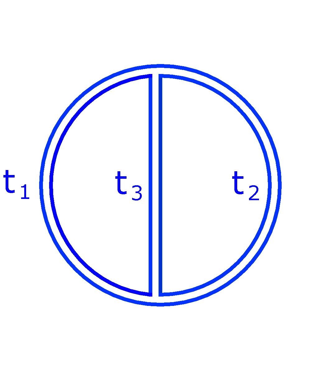
(a)

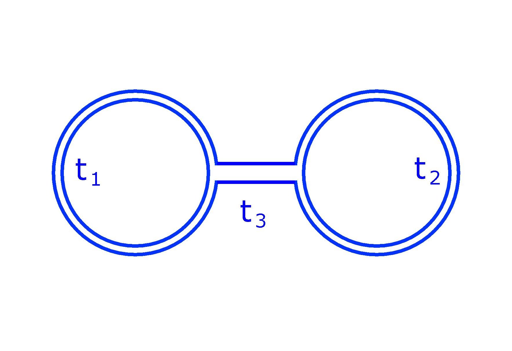
(b)

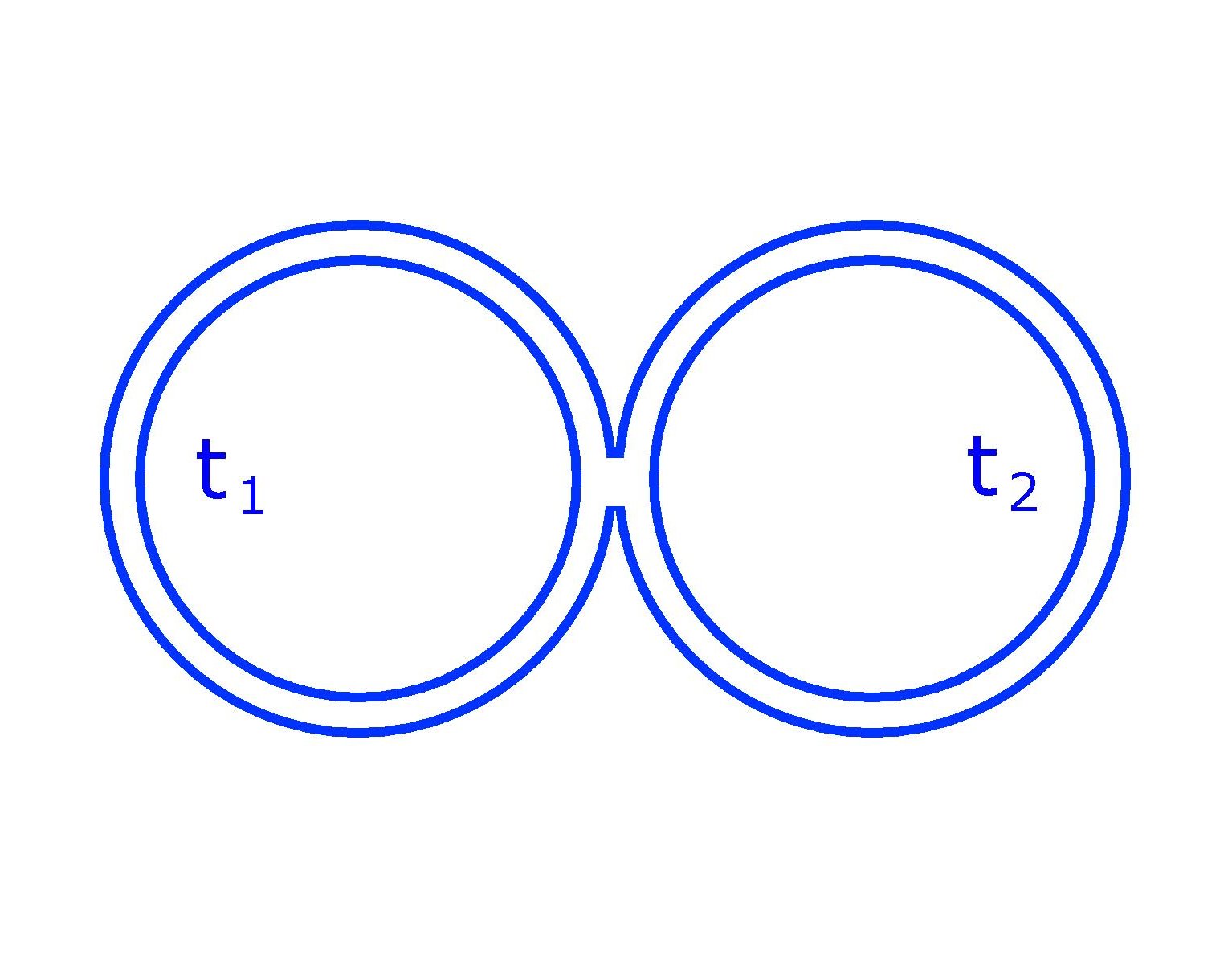
(c)

Figure 1: The three possible degeneration limits of the open string world-sheet for the two-loop vacuum amplitude. Individual propagators are labelled with their Schwinger proper-time variable $t_{i}$.

In these limits, a possible identification between moduli and Schwinger proper times $t_{i}$ for individual propagators is

$$2\pi{\rm i}\tau_{11}\,\simeq\,\log k_{1}\,=\,-\frac{t_{1}+t_{3}}{\alpha^{\prime}}\,,\qquad 2\pi{\rm i}\tau_{22}\,\simeq\,\log k_{2}\,=\,-\frac{t_{2}+t_{3}}{\alpha^{\prime}}\,,$$

$$\hskip 85.35826pt2\pi{\rm i}\tau_{12}\,\simeq\,\log\eta\,=\,-\frac{t_{3}}{\alpha^{\prime}}\,$$ (22)

for Fig. 1a, and

$$2\pi{\rm i}\tau_{11}\,\simeq\,\log k_{1}\,=\,-\frac{t_{1}}{\alpha^{\prime}}\,,\qquad 2\pi{\rm i}\tau_{22}\,\simeq\,\log k_{2}\,=\,-\frac{t_{2}}{\alpha^{\prime}}\,,\qquad\log\left(1-\eta\right)\,=\,-\frac{t_{3}}{\alpha^{\prime}}\,$$ (23)

for Fig. 1b. In the case of the contact interaction of Fig. 1c, no Schwinger proper time is associated to the modulus $\eta$.

This prescription is enough to identify correctly the contributions of the (tachyonic) ground state for bosonic strings, and provides an explicit connections between two-loop string amplitudes and those of a $\phi^{3}$ field theory. One may easily verify that, as shown in Eqns. (22) and (23), the limit $\eta\to 0$ corresponds to the ‘symmetric’ topology shown in Fig. 1a, while the limit $\eta\to 1$ yields the ‘handlebar’ topology of Fig. 1b, as discussed in Ref. Frizzo:1999zx . The first problem we wish to address now is how to generalize the prescriptions in Eqns. (22) and (23), so as to isolate the contributions of the massless degrees of freedom to the various available graph topologies at genus two and higher. Since massless states are not generally the lowest-energy states, corrections to Eqns. (22) and (23) which are subleading by powers of the multipliers may, and do, play a role.

In the present case, the most interesting limit is the ‘symmetric’ topology in Fig. 1a, which we will consider in detail. Our first guiding principle is to connect the sums of all Schwinger proper times forming each loop to the multipliers of some element of the Schottky group. The second key point is that the dictionary between string and field theory quantities must respect the symmetry of the graph representing the degeneration of the Riemann surface, since this symmetry is a remainder of the modular invariance of the original string diagram. At two loops, for the symmetric topology, this is achieved by the following observation. In the Schottky parametrization, acting on the string boundary coordinate with the transformation $S_{i}$ corresponds to moving it around the $i$-th loop once, in a prescribed direction. Similarly, one easily verifies that acting with the transformation $S_{1}S_{2}^{-1}$ corresponds to wrapping once around the outer boundary of the word sheet. In the symmetric topology, these three transformations must be interchangeable, and each one must be associated with the sum of two Schwinger proper times, since each field theory loop is composed of two propagators. These constraints are solved by imposing that

$$k(S_{1})\,=\,p_{1}\,p_{3}\,,\qquad k(S_{2})\,=\,p_{2}\,p_{3}\,,\qquad k(S_{1}S_{2}^{-1})\,=\,p_{1}\,p_{2}\,,$$ (24)

where each $p_{i}$ is then associated with a single field theory propagator, and to the corresponding proper time variable, according to

$$\log p_{i}\,=\,-\,\frac{t_{i}}{\alpha^{\prime}}\,.$$ (25)

Remarkably, the change of variables from the set $\{k_{1},k_{2},\eta\}$ to the set $\{p_{i}\}$ is simple, and one finds

$$\eta\,=\,\frac{(1+p_{1})(1+p_{2})p_{3}}{(1+p_{3})(1+p_{1}p_{2}p_{3})}\,,$$ (26)

which allows us to expand the partition functions in Eq. (12) in a Laurent series in powers of $p_{i}$ without encountering singularities. At leading power in $p_{i}$, the assignment in Eq. (25) coincides with that in Eq. (22). Notice however that, already at next-to-leading power in any of the $p_{i}$, the two choices differ.

In the supersymmetric theory, the approach is similar, but there are also important differences. First of all, the various factors in the partition function must be expanded in powers of $\sqrt{p_{i}}$, instead of $p_{i}$, as can be seen for example in Eq. (18). This means we need to extend equation Eq. (24) to account for the different signs $k_{i}^{{1}/{2}}$. According to the convention explained after (18) we specify

$$k_{1}^{{1}/{2}} =-\sqrt{p_{1}}\sqrt{p_{3}} k_{2}^{{1}/{2}} =-\sqrt{p_{2}}\sqrt{p_{3}} k_{3}^{{1}/{2}}=\big{[}k(S_{1}S_{2}^{-1})\big{]}^{{1}/{2}} =-\sqrt{p_{1}}\sqrt{p_{2}}$$

where all of the $\sqrt{p_{i}}$’s are positive.

More importantly, the standard procedure to extract the field theory limit can be applied only after having performed the Berezin integrations over supermoduli. As noted in Witten:2013cia , it then becomes essential to choose correctly the bosonic moduli that are kept fixed when the Berezin integration is performed. In the present case, one may see that the correct bosonic variable is the quartic invariant $y$ in Eq. (8), and not the closely related one $\eta$. The reason for this is that the bosonic parameter describing the gluing of two punctured annuli that forms our two-loop surface is in fact $y$ Witten:2013cia . In the Schottky approach this can be seen by repeating, in the supersymmetric case, the sewing procedure discussed in Ref. Cristofano:1988cf . In order to extract the field theory limit in the superstring case, we must thus begin by writing the measure of integration in terms of $y$, before performing the integration over the Grassmann parameters. In fact, we expect this prescription to be valid for all values of $y$ that yield a well-defined Riemann surface, and not just around the degeneration point $y=0$. These arguments, which arise from an explicit construction of the two-loop Riemann surface, find a confirmation when the field theory limit is explicitly computed: as we will see in the next section, where we consider the non-separating degeneration $y\to 1$, by using $\eta$ instead of $y$ one gets a result which is inconsistent with basic properties of the low-energy effective theory. By sewing, one constructs an explicit expression for the Schottky generators $\hat{\mathbf{S}}_{1}$, $\hat{\mathbf{S}}_{2}$ of the disk with two holes, as obtained by gluing two annuli with punctures at ${\mathbf{z}}_{1}=(1,\theta_{1})$ and ${\mathbf{z}}_{2}=(1,\theta_{2})$, by means of a propagator of ‘length’ $\log y$. As in the bosonic case Cristofano:1988cf , one finds

$$\hat{\mathbf{S}}_{1}\,=\,{\mathbf{P}}(y)^{-1}\,{\mathbf{V}}_{1}^{-1}\,\mathbf{P}(k_{1})\mathbf{V}_{1}\mathbf{P}(y)\,,\qquad\hat{\mathbf{S}}_{2}\,=\,\mathbf{\Gamma}\,{\mathbf{V}}_{2}^{-1}\,\mathbf{P}(k_{2})\mathbf{V}_{2}\,\mathbf{\Gamma}\,,$$ (27)

where $\mathbf{P}(k_{i})$ are the generators of the two annuli and $\mathbf{P}(y)$ is the propagator which performs the gluing; moreover $\mathbf{V}_{i}$ define local super-coordinates around the two punctures, and the matrix

$${\mathbf{\Gamma}}\,=\,\left(\begin{array}[]{ccc}0&1&0\\ 1&0&0\\ 0&0&1\end{array}\right)\,.$$ (28)

exchanges the origin with the point at infinity.

One can choose the simplest local coordinates, using the supertranslations

$${\mathbf{V}}_{i}\,=\,\left(\begin{array}[]{ccc}1&1&-\theta_{i}\\ 0&1&0\\ 0&\theta_{i}&1\end{array}\right)\,,\qquad$$ (29)

which send the origin to the punctures at ${\mathbf{z}}_{i}$, and one can use the simplest propagator

$${\mathbf{P}}(y)\,=\,\left(\begin{array}[]{ccc}-\sqrt{y}&0&0\\ 0&\frac{-1}{\sqrt{y}}&0\\ 0&0&1\end{array}\right)\,.$$ (30)

In this framework, the Schottky generators $\hat{\mathbf{S}}_{1}$, $\hat{\mathbf{S}}_{2}$ are related by a similarity transformations to the ${\mathbf{S}}_{1}$, ${\mathbf{S}}_{2}$ we will choose in Eq. (40). The gluing parameter $y$ in Eq. (27) is exactly the supersymmetric version of the quartic invariant $y$ introduced in Eq. (8) and is related to the other quartic invariant $\eta$ as

$$\eta\,=\,\big{(}\mathbf{u}_{1},\mathbf{u}_{2},\mathbf{v}_{1},\mathbf{v}_{2}\big{)}\,=\,1-y+\sqrt{\eta}\,\,\Theta_{\mathbf{v}_{1}\mathbf{u}_{1}\mathbf{u}_{2}}\Theta_{\mathbf{v}_{1}\mathbf{u}_{1}\mathbf{v}_{2}}\,.$$ (31)

We can now summarize the prescription for studying the complete degeneration leading to the graph in Fig. 1a: first we have to expand each factor in the measure in a Laurent series in powers of each of the $p_{i}$’s (or $\sqrt{p_{i}}$ in the NS case); then we have to pick the term that cancels all tachyonic poles, so as to have a measure proportional to $dp_{i}/p_{i}=-dt_{i}/\alpha^{\prime}$: indeed, the operator formalism of Ref. DiVecchia:1988cy suggests that in general the propagation of states at the $n$-th mass level of the string should correspond to the term of order $n-2$ in this Laurent series. Finally, in the presence of a background gauge field, we have to rewrite $\epsilon$ in terms of the physical field $B$, by using Eq. (10). At this stage, the field theory integrands for the Feynman diagrams are recovered by taking the limit $\alpha^{\prime}\to 0$, with $B$ and the $t_{i}$’s kept fixed.

By taking the field theory limit as described, string theory yields directly the sum of all Feynman diagrams with the chosen graph topology. For example, both in the bosonic and in the NS cases, each of the three degenerations in Fig. 1 yields a sum of diagrams involving gluons, ghosts, and adjoint scalars. Furthermore, various particles can be charged or neutral with respect to the selected background field, and charged vector particles can be polarized in the ‘magnetized’ $(x_{1},x_{2})$ plane, or in one of the $d-2$ ‘unmagnetized’ directions. One can, however, perform a more detailed analysis. By tracing back the origin of the various factors contributing to the string theory partition function, it is actually possible to disentangle the contributions to each graph topology of each individual particle state, thus extracting directly from string theory the integrands of individual Feynman diagrams. As a byproduct, this leads to the identification of the gauge in which the field theory calculation should be performed to reproduce these results.

The idea is simple. Each factor in the partition functions in Eq. (12) gives a specific contribution, corresponding to the propagation of certain space-time fields and polarizations, which can be identified by recognizing how the factor originates from the path integral over world-sheet fields. First of all, it is natural to identify the factor $F_{\rm scal}$ ($\mathbf{F}_{\rm scal}$ in the supersymmetric case) with the contribution of space-time adjoint scalars, since this factor arises from functional integration over string coordinates with Dirichlet boundary conditions. Thus, if we extract a factor of $p_{i}$ ($\sqrt{p_{i}}$, or a factor quadratic in Grassmannian supermoduli, for the NS case) from this term, we may conclude that the propagator associated with the proper time $t_{i}$ describes a scalar in the corresponding Feynman diagram. Similarly, the factor arising from the functional integral over the world-sheet ghosts $b$ and $c$ must correspond to the space-time propagation of Faddeev-Popov ghosts in the low-energy gauge theory: this identification is supported by comparing the world-sheet and space-time BRST transformations, as done for example in section 4.3 of Ref. Polchinski:1998rq ; we conclude that the expansion of $F_{\rm gh}$ ($\mathbf{F}_{\rm gh}$) will select space-time ghost fields in the corresponding field theory propagators. Finally, the factor $F_{\rm gl}$ ($\mathbf{F}_{\rm gl}$), arising from functional integration over string coordinates with Neumann boundary conditions, yields the gluon contribution to the partition function. In fact, we can distinguish between Feynman diagrams coming from different gluon polarizations: to find the two degrees of freedom parallel to the magnetized ($x_{1}$ $x_{2}$) plane, we extract $p_{i}$ from the $\epsilon$-dependent denominator of Eq. (19), and to get the $(d-2)$ perpendicular degrees of freedom we extract $p_{i}$ from the $\epsilon$-independent terms in the numerator. These give different contributions even if the gluon itself is uncharged with respect to the background field, because of its covariant derivative coupling to charged particles.

While we have described in detail the choice of variables appropriate to the degeneration in Fig. 1a, our approach is completely general and can be extended to other degeneration limits and to higher genus as well. The guiding principles are always the fact that multipliers must be associated with sums of proper time variables for all propagators comprising the loop, and the residual modular symmetries of the diagram must be properly taken into account. These ideas can, for example, be used to analyze the other complete degeneration points at two loops (such as for instance the ‘handlebar’ limit of Fig. 1b), or partial degenerations capturing contributions of diagrams with four-point vertices, as in Fig. 1c. We will discuss in detail the variables appropriate to these cases, and the comparison with the corresponding field theory diagrams, in a forthcoming paper.

5 Extracting Feynman diagrams: an example

To substantiate our arguments in the previous section, we now proceed to extract from the string partition function, in the non-separating degeneration limit depicted in Fig. 1a, the contribution corresponding to a chosen individual Feynman diagram in the low-energy theory. As an example, we select the contribution of charged Faddeev-Popov ghosts circulating in the two external propagators parametrized by $t_{1}$ and $t_{2}$, with a gluon state neutral under the background field $B$ propagating in the middle line parametrized by $t_{3}$. This choice is simple enough to allow for a short derivation and a direct comparison between the bosonic string and the superstring formalisms, and it already contains information about the gauge choice implicit in the string calculation. We postpone the presentation of our detailed analysis of the other diagrammatic contributions to the effective action to a future publication.

As discussed in the previous section, for the symmetric topology in Fig. 1a we need to use the variables $\{p_{i}\}$ defined in Eq. (24). In the bosonic case, it is straightforward to rewrite the zero-mode part of the ghost measure $F_{\rm gh}$ in Eq. (14) in terms of these variables. One finds

$$\frac{dk_{1}}{k_{1}^{2}}\,\frac{dk_{2}}{k_{2}^{2}}\,\frac{d\eta}{(1-\eta)^{2}}(1-k_{1})^{2}(1-k_{2})^{2}\,=\,\frac{dp_{1}}{p_{1}^{2}}\,\frac{dp_{2}}{p_{2}^{2}}\,\frac{dp_{3}}{p_{3}^{2}}\,(1-p_{2}p_{3})(1-p_{1}p_{3})(1-p_{1}p_{2})\,.$$ (32)

One immediately notices the complete symmetry of this expression under permutations of the $p_{i}$’s, which is a pre-requisite for the consistency of the field theory limit for the symmetric topology. One also notes the absence of terms linear in only one of the $p_{i}$’s, which corresponds to the absence of diagrams with a single ghost propagator in the gauge theory. To pick our chosen diagram, we must compensate the quadratic poles in $p_{1}$ and $p_{2}$ by taking the term linear in $p_{1}p_{2}$ from $F_{\rm gh}$. This is completely given in Eq. (32), as one easily sees that the infinite product in the first line of Eq. (14) contributes terms which are at least quadratic in the $p_{i}$’s. In order to complete the calculation, we must next select the term linear in $p_{3}$, but without any powers of $p_{1}$ and $p_{2}$, from the gluon factor $F_{\rm gl}^{(\epsilon)}$. In order to do this, we need the approximate expressions for the only two objects that remain non-trivial when we set $p_{1}$ and $p_{2}$ to zero: the determinant of the period matrix $\det\tau$, and its twisted version, $\det\tau_{\epsilon}$. We can extract these results from Magnea:2004ai ; Russo:2007tc . Up to corrections vanishing as powers of $p_{1}$ or $p_{2}$, the elements of the period matrix are

$$2\pi i\tau_{11}\,=\,\log(p_{1}p_{3})\,,\qquad 2\pi i\tau_{22}\,=\,\log(p_{2}p_{3})\,,\qquad 2\pi i\tau_{12}\,=\,2\pi i\tau_{21}\,=\,\log\eta\,.$$ (33)

Furthermore, the expression for the determinant of the twisted period matrix, at leading power in $p_{1}$ and $p_{2}$ and including the linear term in $p_{3}$, is given in the limit $\epsilon_{2}\to-\epsilon\,,\,\epsilon_{1}\to\epsilon$, as

$${\rm Im}(\tau_{\epsilon}) = \frac{1}{4\pi\sin(\pi\epsilon)}\,\Bigg{[}\frac{1}{\epsilon}\,\left(p_{1}^{\epsilon/2}-p_{1}^{-\epsilon/2}\right)\left(p_{2}^{\epsilon/2}-p_{2}^{-\epsilon/2}\right)+\,\Big{(}2\gamma_{E}+\log p_{3}+\psi(-\epsilon)+\psi(\epsilon)\Big{)}$$ (34)

$$\times\,\left(\left(p_{1}^{\epsilon/2}p_{2}^{\epsilon/2}-p_{1}^{-\epsilon/2}p_{2}^{-\epsilon/2}\right)-\epsilon p_{3}\left(p_{1}^{\epsilon/2}p_{2}^{-\epsilon/2}+p_{1}^{-\epsilon/2}p_{2}^{\epsilon/2}\right)\right)\Bigg{]}~{},$$

where $\psi(z)=\Gamma^{\prime}(z)/\Gamma(z)$ is the digamma function and $\gamma_{E}=-\psi(1)$ is the Euler-Mascheroni constant. Both expressions must be written in terms of $p_{i}$, and to extract our chosen diagram we must further expand in powers of $p_{3}$ and pick the term linear in $p_{3}$. The leading order in $p_{3}$ of Eq. (34) is given by Eq. (4.7) of Russo:2007tc ; it is possible to generalise that derivation to include also the subleading term which is proportional to $p_{3}$. However there is an alternative, simpler approach and we will come back to this point in a subsequent paper. Assembling the various factors, and including the overall normalization $C_{g}(\vec{\epsilon})$, it is then straightforward to take the $\alpha^{\prime}\to 0$ limit, which yields the expression for our chosen diagram, which we label by $D_{\rm gh}^{\rm sym}(B)$. We find

$$D_{\rm gh}^{\rm sym}(B)\,=\,K\,\frac{g^{2}}{(4\pi)^{d}}\,\int_{0}^{\infty}\left[\prod_{i=1}^{3}dt_{i}\right]\frac{t_{3}}{\Delta_{0}^{d/2}\,\Delta_{B}}\Bigg{\{}\frac{d-2}{2}+\frac{\Delta_{0}}{\Delta_{B}}\,\cosh\big{(}B(t_{1}-t_{2})\big{)}\Bigg{\}}\,,$$ (35)

where $g$ is the gauge theory coupling, $K$ is a normalization factor to be discussed below, and we introduced the notations

$$\Delta_{B} \equiv \frac{1}{B^{2}}\Big{[}\sinh(Bt_{1})\sinh(Bt_{2})\,+\,t_{3}B\sinh\big{[}B(t_{1}+t_{2})\big{]}\Big{]}\,,$$

$$\Delta_{0} \equiv \lim_{B\to 0}\Delta_{B}\,=\,t_{1}t_{2}+t_{1}t_{3}+t_{2}t_{3}\,.$$ (36)

These are related to the period matrix and to the twisted period matrix, after making the substitutions in Eq. (10) and Eq. (25), via

$$\Delta_{B}\,=\,\lim_{\alpha^{\prime}\to 0}\,\left[\left(2\pi\alpha^{\prime}\right)^{2}\,\det\left({\rm Im}\tau_{\epsilon}\right)\right]\,,\qquad\Delta_{0}\,=\,\lim_{\alpha^{\prime}\to 0}\,\left[\left(2\pi\alpha^{\prime}\right)^{2}\,{\rm det}\left({\rm Im}\tau\right)\right]\,.$$ (37)

In Eq. (35), one easily identifies the first term in braces as related to the $d-2$ gluon polarizations along ‘neutral’ directions, while the remaining term comes from gluons polarized in the ‘magnetized’ $(x_{1}x_{2})$ plane.

In quantum field theory, the precise value, and in fact the very existence, of diagrams like the one just discussed, depends of course on the gauge choice. For the particular diagram we are considering, it turns out that the structure of the integrand in Eq. (35) follows from the standard choice of the Feynman gauge, see Pawlowski:2008xh (the diagram we considered corresponds to the terms with an explicit ${\cal F}^{2}$ in the integrand ${\cal I}_{\rm ghost}$ in Pawlowski:2008xh ; the remaining contributions are related to the diagram with a neutral ghost and a charged gluon). Even for this simple diagram, however, in order to recover the correct normalization we find that the gauge choice must be modified. In order to identify the gauge, we have performed the calculation of the effective action in the background field $B$, using the background field method, as described in Abbott:1980hw , but with the non-linear covariant gauge-fixing choice suggested by Bern:1991an , which evolves out of the Gervais-Neveu gauge first identified in Ref. Gervais:1972tr . While leaving a detailed analysis of the gauge choice on the field theory side to future work, we note here that the correct choice is to pick the gauge fixing Lagrangian

$${\cal L}_{\rm GF}\,=\,-\,{\rm Tr}\left[{\cal G}^{2}\left({\cal A},{\cal Q}\right)\right]\,,$$ (38)

where ${\cal A}$ is the background field, ${\cal Q}$ the quantum field, and

$${\cal G}\left({\cal A},{\cal Q}\right)\,=\,D_{\mu}^{\cal A}{\cal Q}^{\mu}+\frac{\rm i}{2}\gamma g\left\{{\cal Q},{\cal Q}\right\}\,,$$ (39)

with $D_{\mu}^{\cal A}$ the covariant derivative with respect to the background field. If one computes, for example, the diagram $D_{\rm gh}^{\rm sym}(B)$ in this gauge, one finds precisely the structure of Eq. (35), with an overall normalization $K=1+\gamma^{2}$. We have checked that the string theory results reproduce all gauge theory diagrams, as for the ghost diagram, with the choice $\gamma^{2}=1$ (note that the sign of $\gamma$ is immaterial, since $\gamma$ appears only quadratically in all diagrams).

Let us now outline the analysis of the same example from the superstring point of view. As discussed in the previous section, the Berezin integration should be defined by keeping constant the bosonic variable $y$. Instructed by the bosonic case, we know that the complete degeneration depicted in Fig. 1a is described in terms of the variables $p_{i}$, where however the definition in Eq. (24) now involves the multipliers of super-Schottky transformations. We need thus to write the supersymmetric analogue of Eq. (26). For for simplicity, we fix our global super-projective coordinates by choosing $\mathbf{u_{1}}=(0,0)$, $\mathbf{v_{1}}=(\infty,0)$, $\mathbf{u_{2}}=(u,\theta)$, and $\mathbf{v_{2}}=(1,\phi)$. This implies

$$\eta\,=\,u\,,\ \Theta_{\mathbf{v}_{1}\mathbf{u}_{1}\mathbf{u}_{2}}\,=\,\theta/\sqrt{u}\,,\qquad\Theta_{\mathbf{v}_{1}\mathbf{u}_{1}\mathbf{v}_{2}}\,=\,\phi\,.$$ (40)

If we use $k_{3}^{{1}/{2}}$ to denote the smallest (in absolute value) eigenvalue of $\mathbf{S}_{1}\mathbf{S}_{2}^{-1}$ (so $k_{3}$ is its multiplier), we can express $y$ as

$$y\,=\,\frac{(1-k_{1})(1-k_{2})\,+\,\theta\,\phi\,\Big{[}(1-{\rm e}^{{\rm i}\pi\varsigma_{1}}k_{1}^{{1}/{2}})(1-{\rm e}^{{\rm i}\pi\varsigma_{1}}k_{2}^{{1}/{2}})(1+{\rm e}^{{\rm i}\pi(\varsigma_{1}+\varsigma_{2})}k_{1}^{{1}/{2}}k_{2}^{{1}/{2}})\Big{]}}{1+k_{1}k_{2}-k_{1}^{{1}/{2}}k_{2}^{{1}/{2}}(k_{3}^{{1}/{2}}+k_{3}^{-{1}/{2}})}\,.$$ (41)

With our choice of coordinates, the prefactor in the supersymmetric measure of integration given in square brackets in Eq. (15) takes a particularly simple form, and can be written as

$$\frac{dk_{1}}{k_{1}^{3/2}}\,\frac{dk_{2}}{k_{2}^{3/2}}\,\,d\log y\,d\theta\,d\phi\,=\,\frac{dp_{1}}{p_{1}^{3/2}}\,\frac{dp_{2}}{p_{2}^{3/2}}\,\frac{dp_{3}}{p_{3}}\,d\theta\,d\phi\,\,\frac{1-p_{1}p_{2}}{(1+p_{3})(1+p_{1}p_{2}p_{3})}\,.$$ (42)

Contrary to the bosonic result, Eq. (32), this expression is not symmetric under permutations of the $p_{i}$, and it does not become symmetric even after including the zero-mode contribution of the ghost sectors, given by the first factor in $\mathbf{F}_{\rm gh}$ in Eq. (18). Fortunately, we can restore the symmetry, and the one-to-one correspondence between string and field theory integrands, by exploiting the freedom to rescale Grassmann variables in the Berezin integral. We do so by defining

$$\hat{\theta}_{ij}\,=\,c_{ij}\,\Theta_{\mathbf{v}_{i}\mathbf{u}_{i}\mathbf{u}_{j}}\,,\qquad\hat{\phi}_{ij}\,=\,c_{ij}\,\Theta_{\mathbf{v}_{i}\mathbf{u}_{i}\mathbf{v}_{j}}\,,$$ (43)

where

$$c_{12}\,=\,\left[\left(1+{\rm e}^{{\rm i}\pi\varsigma_{3}}\sqrt{p_{1}}\sqrt{p_{2}}\right)\left(1-{\rm e}^{{\rm i}\pi\varsigma_{1}}\sqrt{p_{1}}\sqrt{p_{3}}\right)\left(1-{\rm e}^{{\rm i}\pi\varsigma_{2}}\sqrt{p_{2}}\sqrt{p_{3}}\right)\right]^{-1/2}\,,$$ (44)

with $c_{23}$ and $c_{31}$ obtained by permuting the indices $(123)$. As before, $\varsigma_{3}=\varsigma_{1}+\varsigma_{2}$, $\mathbf{u}_{3}$ and $\mathbf{v}_{3}$ label respectively the spin structure and the fixed points of the transformation $\mathbf{S}_{1}\mathbf{S}_{2}^{-1}$. In terms of these new Grassmann variables, Eq. (42), multiplied times the zero-mode contribution of the ghost sectors in Eq. (18), reads

$$\prod_{i=1}^{3}\left[\frac{dp_{i}}{p_{i}^{3/2}}\,\frac{1+{\rm e}^{{\rm i}\pi\varsigma_{i}}k_{i}^{{1}/{2}}}{\sqrt{1+p_{i}}}\right]d\hat{\theta}_{12}\,d\hat{\phi}_{12}\,\frac{1}{\sqrt{1+p_{1}p_{2}p_{3}}}\,,$$ (45)

which is the supersymmetric analogue of Eq. (32). One can check that $d\hat{\theta}_{12}d\hat{\phi}_{12}\,=\,d\hat{\theta}_{23}d\hat{\phi}_{23}\,=\,d\hat{\theta}_{31}d\hat{\phi}_{31}$, so that Eq. (45) is fully symmetric under permutations of the super-Schottky transformations $\mathbf{S}_{i}$ as expected.

We can now easily derive the result in Eq. (35) from the superstring partition function $\mathbf{Z}(B)$ in Eq. (12). We first isolate the term proportional to $\sqrt{p_{1}p_{2}}$ in the ghost contribution (45). As before, this corresponds to selecting the contribution of space-time ghosts in the external loop of the diagram in Fig. 1a. Next we must expand $\mathbf{F}_{\rm gl}^{(\epsilon)}$ to first order in $\sqrt{p_{3}}$ and to zeroth order in $\sqrt{p_{1}}$ and $\sqrt{p_{2}}$. As in the bosonic case, terms of this type can arise only from the expansion of the super period matrix, both in the twisted and in the untwisted version. As before, the first case corresponds, on the field theory side, to contributions due to the propagation, in the middle propagator of Fig. 1a, of a gluon neutral with respect to the background field $B$, and with a polarization parallel to the magnetised plane, while the second case corresponds to perpendicular polarizations. It is straightforward to supersymmetrize the standard and the twisted period matrix and repeat the steps outlined in Magnea:2004ai ; Russo:2007tc to calculate the superperiods at zeroth order in $p_{1}$ and $p_{2}$. Indeed, at this order, the result for the untwisted period matrix in terms of $\eta$ is identical to the bosonic one, provided super fixed points and supersymmetric differences $\langle{\mathbf{z}_{1}}|{\mathbf{z}_{2}}\rangle$ are used in place of bosonic ones. On the other hand, at this order the twisted superperiod matrix has a term linear in $\theta\phi$, when written in terms of $\eta$. Our final ingredient is the expression for $\eta$ in the supersymmetric case: by using Eq. (40) and Eq. (41) we find

$$\eta\,=\,\frac{p_{3}}{1+p_{3}}(1+\theta\phi)+{\cal O}(\sqrt{p_{1}},\sqrt{p_{2}})\,=\,{p_{3}}\left(1+\sqrt{p_{3}}\,\hat{\theta}_{12}\,\hat{\phi}_{12}\right)+{\cal O}(\sqrt{p_{1}},\sqrt{p_{2}},p_{3}^{2})\,.$$ (46)

This has to be compared with Eq. (26) in the bosonic case, after expansion in powers of $p_{3}$, which yields $\eta=p_{3}(1-p_{3})+{\cal O}(p_{1},p_{2},p_{3}^{3})$. The integrands have both analytic and logarithmic (e.g. $\eta^{\epsilon}$) dependence on $\eta$. The term coming from the logarithmic dependence of $\mathbf{F}_{\rm gl}^{(\epsilon)}$ on $\eta$ which is linear in $\hat{\theta}_{12}\hat{\phi}_{12}$ has the same structure as the first-order term coming from the logarithmic dependence in the expansion of ${F}_{\rm gl}^{(\epsilon)}$, except for the fact that it is proportional to $\sqrt{p_{3}}$ instead of $p_{3}$. It also turns out that the linear term in $\theta\phi$ in the twisted superperiod matrix has the same form as the linear term in $\eta$ in the twisted period matrix, so when we write $\theta\phi=\sqrt{p_{3}}\hat{\theta}_{12}\hat{\phi}_{12}+{\cal O}(\sqrt{p_{1}},\sqrt{p_{2}},p_{3})$ we see that the untwisted and twisted superperiod matrices are almost identical except the linear terms in $p_{3}$ are instead proportional to $\sqrt{p_{3}}\hat{\theta}_{12}\hat{\phi}_{12}$. This, however, is exactly what we need in order to compensate the tachyonic pole in the superstring measure in (45), so that finally we reproduce exactly the field theory result in Eq. (35).

Let us conclude this section by analysing what happens if we change our local coordinates on supermoduli space and choose, for instance, to fix the bosonic modulus $\eta$ (instead of $y$) in the Berezin integration. It is straightforward to check that this corresponds to the choice of Ref. D'Hoker:2002gw , at least at leading order in the $\tau_{ij}\to{\rm i}\infty$ limit, for the two-loop vacuum amplitude at $\epsilon=0$. With this choice, it is not possible to trace a one-to-one correspondence between each Feynman diagram and individual contributions to the string amplitudes. However, even without aiming at separating different diagrams, we can still ask whether we can interpret from a field theory point of view the leading contribution to the symmetric graph topology in the $B\to 0$ limit. We would expect to find a correspondence with a diagram similar to the one discussed in this paper, where ghost lines have been substituted by NS tachyon propagators, while the third propagator is still a gluon. Now, the main feature of the result obtained by keeping $\eta$ fixed is that the integrand of each NS spin structure in the complete degeneration limit is proportional to $\Delta_{0}^{-d/2}$. Any sensible interaction term with two scalar particles and a gluon must however involve a derivative, which inevitably leads to a numerator linear in the appropriate Schwinger parameter in the diagram integrand. In field theory, it thus appears impossible to generate this dependence on $\Delta_{0}$, which is typical of non-derivative couplings. This is to be contrasted with the integrand obtained by using $y$ in the Berezin integration, which is proportional to $t_{3}/\Delta_{0}^{d/2+1}$, as one finds in the $\epsilon\to 0$ limit of Eq. (35), and as expected from the coupling structure of the low-energy gauge theory.

6 Conclusions

In this paper we have shown how to parametrize a Riemann surface describing a degenerating multi-loop string amplitude, so as to make explicit contact with the corresponding Feynman diagrams of the low-energy quantum field theory. We have been working in the RNS formalism, and we found the Schottky parametrization of (super) Riemann surfaces to be especially suited to study the correspondence between string and field theory amplitudes. We have proposed an essentially algorithmic procedure that allows us to start from the full expression for an open string amplitude, as an integral over (super) moduli space, and derive from it the corresponding gauge theory amplitude on a diagram-by-diagram basis. In the present paper we focused on issues concerning the parametrization of the string world sheet, and on the comparison between the bosonic string setting and the NS sector of the superstring. To this end, we used, as an example of our technique, the study of string effective actions in a constant background gauge field, and, in the process, we also presented some new results concerning the multi-loop expression for this effective action for the NS spin structure of the superstring. To illustrate our results, we have presented a relatively simple example, deriving explicitly from the two-loop string partition function a specific two-loop Feynman diagram involving a loop of space-time ghosts and a gluon propagator. We leave to forthcoming papers a detailed analysis of specific 4D field theories, and the discussion of several issues relevant to the field theory description emerging from the string amplitudes, such as the regularization of IR divergences, the precise gauge fixing procedure, and the most convenient approach to renormalisation. In this concluding section we would like to make some general remarks about what can be learnt from the study of multi-loop (super)string amplitudes in the degeneration limit.

A first interesting point is that, in the low energy limit, we are able to obtain from string amplitudes a set of field theory quantities, such as the Schwinger-parameter integrands of individual Feynman diagrams, which contain off-shell information, allowing for example to infer the Feynman rules of the low-energy theory. We note that this relation works with the specific set of coordinates we used in the degeneration limit, and with a specific choice of gauge on the field theory side. Perhaps not surprisingly, the gauge we identified is a natural generalization of the non-linear gauge found in the study of tree-level string amplitudes in Ref. Gervais:1972tr , as first suggested in Ref. Bern:1991an . Interestingly, it does not seem possible to modify in a simple way the approach on either side of the correspondence. For instance, as discussed at the end of the previous section, a different choice for Berezin integration yields, in the complete degeneration limit, results that are difficult to interpret from the field theory point of view. Similarly, there is no obvious way to change the choice of gauge one finds on the field theory side, at least within the framework of covariant string quantization. We recall that, on the other hand, strings quantized on the light cone Goddard:1973qh ; Thorn:2002fj result in quantum-field theory amplitudes computed in a physical light-cone gauge.

Another important feature of our result is that it is very flexible, and works in setups with a different number of Neumann and Dirichlet directions, and different brane configurations. Here we considered the case where the low energy theory describing massless open string states is a Yang-Mills theory in $D=26$ ($D=10$ super Yang-Mills theory in the superstring case), reduced to $d$ space-time dimensions. We note that actually the number $s$ of scalar states (and thus the number of space-time supersymmetries in the case of RNS string theory) present in the low-energy theory can be easily tuned by introducing orbifold projections to reduce their number below the one dictated by the critical dimension. In a similar vein, we expect that our approach can be extended to higher-genus Riemann surfaces, and to scattering amplitudes with massless external states. It is reasonable to expect that similar techniques could be used to calculate closed string amplitudes, yielding expressions for graviton scattering amplitudes in a variety of gravity theories.

Finally, even in the simplest case, where no orbifold projection is considered, it is interesting to study explicitly the twisted string partition function discussed in this paper for different values of $d$. For instance, while $d=4$ is obviously relevant for making contact with four-dimensional gauge theories, the choice $d=1$ describes the dynamics of D$0$-branes. In this setting, one should analytically continue the twist parameter $\epsilon\to{\rm i}\epsilon$ to describe the relative velocities between different D$0$-branes; this case was studied in detail in the context of the BFFS model in Ref. Banks:1996vh . At the one-loop level we know exact string results Bachas:1995kx ; Billo:1997eg that interpolate between the open string/M(atrix) limit and the closed string/gravity limit. At two loops, the two limits were studied in detail in Okawa:1998pz , but no full string derivation is known. After including the contribution of the Ramond spin structures, our approach should simplify the comparison between the full two-loop string partition function and the formulae describing the interaction of three moving D$0$-branes in an appropriate limit; this should provide stringent checks on whether all the subtleties of RNS multi-loop amplitudes have been properly resolved. We plan to address this range of interesting open issues in our future work.

Acknowledgements.

We would like to thank C. Bachas and P. Di Vecchia for enlightening discussions. This work was supported by STFC (Grant ST/J000469/1, ‘String theory, gauge theory & duality’) and by MIUR (Italy) under contracts 2006020509$\_$004 and 2010YJ2NYW$\_$006. L. M. and S. Sc. are very grateful to CERN and to QMUL for hospitality during the completion of this work; L. M. also thanks NIKHEF (Amsterdam) for hospitality and support. R. R. wishes to thank Université Pierre et Marie Curie (Paris) and Università di Torino for hospitality, and the ‘Institut Lagrange de Paris’ for support during the completion of this work. S. P. also thanks Università di Torino for hospitality.

References

- (1) V. Alessandrini and D. Amati, Properties of dual multiloop amplitudes, Nuovo Cim. A4 (1971) 793–844.
- (2) E. P. Verlinde and H. L. Verlinde, Multiloop Calculations in Covariant Superstring Theory, Phys.Lett. B192 (1987) 95.
- (3) E. D’Hoker and D. Phong, The Geometry of String Perturbation Theory, Rev.Mod.Phys. 60 (1988) 917.
- (4) E. D’Hoker and D. Phong, Lectures on two loop superstrings, Conf.Proc. C0208124 (2002) 85–123, [hep-th/0211111].
- (5) E. Witten, Superstring Perturbation Theory Revisited, 1209.5461.
- (6) J. Scherk, Zero-slope limit of the dual resonance model, Nucl.Phys. B31 (1971) 222–234.
- (7) J.-L. Gervais and A. Neveu, Feynman rules for massive gauge fields with dual diagram topology, Nucl.Phys. B46 (1972) 381–401.
- (8) M. L. Mangano, S. J. Parke, and Z. Xu, Duality and Multi-gluon Scattering, Nucl.Phys. B298 (1988) 653.
- (9) Z. Bern and D. A. Kosower, The Computation of loop amplitudes in gauge theories, Nucl.Phys. B379 (1992) 451–561.
- (10) Z. Bern, L. J. Dixon, and D. A. Kosower, One loop corrections to five gluon amplitudes, Phys.Rev.Lett. 70 (1993) 2677–2680, [hep-ph/9302280].
- (11) Z. Bern, D. C. Dunbar, and T. Shimada, String based methods in perturbative gravity, Phys.Lett. B312 (1993) 277–284, [hep-th/9307001].
- (12) P. Di Vecchia, L. Magnea, A. Lerda, R. Russo, and R. Marotta, String techniques for the calculation of renormalization constants in field theory, Nucl.Phys. B469 (1996) 235–286, [hep-th/9601143].
- (13) A. Frizzo, L. Magnea, and R. Russo, Scalar field theory limits of bosonic string amplitudes, Nucl.Phys. B579 (2000) 379–410, [hep-th/9912183].
- (14) A. Frizzo, L. Magnea, and R. Russo, Systematics of one loop Yang-Mills diagrams from bosonic string amplitudes, Nucl.Phys. B604 (2001) 92–120, [hep-ph/0012129].
- (15) R. Metsaev and A. A. Tseytlin, On loop corrections to string theory effective actions, Nucl.Phys. B298 (1988) 109.
- (16) C. Bachas and M. Porrati, Pair creation of open strings in an electric field, Phys.Lett. B296 (1992) 77–84, [hep-th/9209032].
- (17) L. Magnea, R. Russo, and S. Sciuto, Two-loop Euler-Heisenberg effective actions from charged open strings, Int.J.Mod.Phys. A21 (2006) 533–558, [hep-th/0412087].
- (18) R. Russo and S. Sciuto, The Twisted open string partition function and Yukawa couplings, JHEP 0704 (2007) 030, [hep-th/0701292].
- (19) G. V. Dunne, Heisenberg-Euler effective Lagrangians: Basics and extensions, hep-th/0406216.
- (20) L. Alvarez-Gaume, C. Gomez, G. W. Moore, and C. Vafa, Strings in the Operator Formalism, Nucl.Phys. B303 (1988) 455.
- (21) P. Di Vecchia, F. Pezzella, M. Frau, K. Hornfeck, A. Lerda, and S. Sciuto, N-point g-loop vertex for a free bosonic theory with vacuum charge Q, Nucl.Phys. B322 (1989) 317.
- (22) L. Alvarez-Gaume, C. Gomez, P. C. Nelson, G. Sierra, and C. Vafa, Fermionic strings in the operator formalism, Nucl.Phys. B311 (1988) 333.
- (23) Z. Bern and D. C. Dunbar, A Mapping between Feynman and string motivated one loop rules in gauge theories, Nucl.Phys. B379 (1992) 562–601.
- (24) E. Witten, More On Superstring Perturbation Theory, 1304.2832.
- (25) E. Witten, Notes On Super Riemann Surfaces And Their Moduli, 1209.2459.
- (26) E. J. Martinec, Conformal Field Theory on a (Super)Riemann Surface, Nucl.Phys. B281 (1987) 157.
- (27) A. Neveu and P. C. West, Neveu-Schwarz excited string scattering: a superconformal group computation, Phys.Lett. B200 (1988) 275.
- (28) P. Di Vecchia, K. Hornfeck, M. Frau, A. Lerda, and S. Sciuto, N-string, g-loop vertex for the fermionic string, Phys.Lett. B211 (1988) 301.
- (29) K. Hornfeck, Three reggeon light cone vertex of the Neveu-Schwarz string, Nucl.Phys. B293 (1987) 189.
- (30) P. Di Vecchia, M. Frau, A. Lerda, and S. Sciuto, A simple expression for the multiloop amplitude in the bosonic string, Phys.Lett. B199 (1987) 49.
- (31) R. Russo and S. Sciuto, Twisted determinants on higher genus Riemann surfaces, Nucl.Phys. B669 (2003) 207–232, [hep-th/0306129].
- (32) P. Di Vecchia, L. Magnea, A. Lerda, R. Marotta, and R. Russo, Two loop scalar diagrams from string theory, Phys.Lett. B388 (1996) 65–76, [hep-th/9607141].
- (33) G. Cristofano, F. Nicodemi, and R. Pettorino, Covariant basic operators in bosonic string theory, Int.J.Mod.Phys. A4 (1989) 857–871.
- (34) J. Polchinski, String theory. Vol. 1: An introduction to the bosonic string, .
- (35) J. M. Pawlowski, M. G. Schmidt, and J.-H. Zhang, On the Yang-Mills two-loop effective action with wordline methods, Phys.Lett. B677 (2009) 100–108, [0812.0008].
- (36) L. Abbott, The Background Field Method Beyond One Loop, Nucl.Phys. B185 (1981) 189.
- (37) P. Goddard, J. Goldstone, C. Rebbi, and C. B. Thorn, Quantum dynamics of a massless relativistic string, Nucl.Phys. B56 (1973) 109–135.
- (38) C. B. Thorn, A World sheet description of planar Yang-Mills theory, Nucl.Phys. B637 (2002) 272–292, [hep-th/0203167].
- (39) T. Banks, W. Fischler, S. Shenker, and L. Susskind, M theory as a matrix model: A Conjecture, Phys.Rev. D55 (1997) 5112–5128, [hep-th/9610043].
- (40) C. Bachas, D-brane dynamics, Phys.Lett. B374 (1996) 37–42, [hep-th/9511043].
- (41) M. Billo, P. Di Vecchia, and D. Cangemi, Boundary states for moving D-branes, Phys.Lett. B400 (1997) 63–70, [hep-th/9701190].
- (42) Y. Okawa and T. Yoneya, Multibody interactions of D particles in supergravity and matrix theory, Nucl.Phys. B538 (1999) 67–99, [hep-th/9806108].