Transport of spin-anisotropy without spin currents

Abstract

We revisit the transport of spin-degrees of freedom across an electrically and thermally biased tunnel junction between two ferromagnets with non-collinear magnetizations. Besides the well-known charge and spin currents we show that a non-zero spin-quadrupole current flows between the ferromagnets. This tensor-valued current describes the non-equilibrium transport of spin-anisotropy relating to both local and non-local multi-particle spin correlations of the circuit. This quadratic spin-anisotropy, quantified in terms of the spin-quadrupole moment, is fundamentally a two-electron quantity. In spin-valves with an embedded quantum dot such currents have been shown to result in a quadrupole accumulation that affects the measurable quantum dot spin and charge dynamics. The spin-valve model studied here allows fundamental questions about spin-quadrupole storage and transport to be worked out in detail, while ignoring the detection by a quantum dot. This physical understanding of this particular device is of importance for more complex devices where spin-quadrupole transport can be detected. We demonstrate that, as far as storage and transport are concerned, the spin anisotropy is only partly determined by the spin polarization. In fact, for a thermally biased spin-valve the charge- and spin-current may vanish, while a pure exchange spin-quadrupole current remains, which appears as a fundamental consequence of Pauli’s principle. We extend the real-time diagrammatic approach to efficiently calculate the average of multi-particle spin-observables, in particular the spin-quadrupole current. Although the paper addresses only leading order and spin-conserving tunneling we formulate the technique for arbitrary order in an arbitrary, spin-dependent tunnel coupling in a way that lends itself to extension to quantum-dot spin-valve structures.

I Introduction

Spintronics combines the concepts of electronic transport and spin physics. One of the earliest examples in solid state physics was the tunnel magnetoresistance effect, discovered by Julliere in 1975 M. Julliere (1975): the charge current through two tunnel-coupled ferromagnets decreases when their magnetizations are changed from a parallel to an antiparallel configuration. The simple explanation of Julliere M. Julliere (1975), based on the spin-dependence of the density of states for spin-$\uparrow$ and $\downarrow$, has been refined and extended by later works. Slonczewski calculated  the spin current through the FM-I-FM junction  J. C. Slonczewski (1989), which can be detected by a second tunnel junction Potok et al. (2002). The spin current is responsible for an exchange coupling between magnetizations of the two ferromagnets Braun et al. (2005); J. C. Slonczewski (1989)). An important early application of spin currents is spin injection from ferromagnets into non-magnetic systems, (for a review see Schmidt (2005)).

Since then, the frontiers of spintronics have been pushed more and more towards the nanoscale, in particular by attaching macroscopic leads to small quantum dots. To name only a few interesting effects in which the transport heavily relies on the spin physics, we mention the Kondo effect Glazman and Raikh (1988); Goldhaber-Gordon et al. (1998), Pauli blockade K. Ono et al. (2002), and various types of spin-blockade effects Weinmann et al. (1994). The spintronic features mentioned for the mesoscopic systems also have a counterpart in microscopic quantum dot physics. For instance, spin injection into quantum dots and spin currents have been measured Chye et al. (2002). Moreover, for non-collinearly magnetized ferromagnets, the above mentioned exchange effects translates into a dipolar exchange field Braun et al. (2004), which can even lift the spin-valve effect.

Besides these analogies, there are, however, profound differences when microscopic systems such as quantum dots are involved. Due to the spatial confinement of electrons, Coulomb electron-electron interaction becomes all-important and correlations between electrons play a prominent role. Spin correlations are built up due to the exchange spin-spin interaction, which results from the concerted action of charging effects and the Pauli principle. This couples the spin-dipole moments of the individual electrons to high-spin states ($S\geqslant 1$). Such high-spin quantum systems have non-trivial higher spin-moments beyond the average spin, such as the spin-quadrupole moment (SQM), which is usually the dominant part. In the physical language of atomic and molecular magnetism, the SQM characterizes the quadratic spin anisotropy. It quantifies the preference of pairs of spins that make up the large moment $S\geqslant 1$ to be aligned along a specific axis irrespective of their orientation along this axis (up, down). SQM is also relevant to transport: for example, a spin anisotropy barrier can completely determine the signatures of the conductance through molecule magnets D. Gatteschi and Villain (2006) and magnetic adatoms Brune and Gambardella (2009). However, in these devices the spin anisotropy appears rather as a property  “fixed”  to the atoms/molecule and not something that could be moved around. This latter idea has been introduced by recent publications Sothmann and König (2010); Baumgärtel et al. (2011); Misiorny et al. (2012a), which point out that spin-quadrupole moment, like spin-dipole moment, can be injected and accumulated in a high-spin quantum dot attached to ferromagnets. Thus, spin anisotropy has turned out to be a true transport quantity in some ways similar to spin-dipole moment. Thus, the transport picture of spin degrees of freedom needs to be extended beyond that offered by charge and spin currents. This is at the heart of this paper, which studies the storage and transport of spin-quadrupole moment in spintronic devices, merging concepts of spintronics and electron-spin correlations (for example present in single-molecule magnets). The aim of this paper is to answer the following three fundamental questions raised by the above cited studies:

i. How is SQM stored in macroscopic system, i. e., ferromagnets?

ii. How is SQM transported macroscopically between such reservoirs?

iii. How can one define an SQM current operator and what is the physical interpretation of its average?

The answers are by no means obvious since SQM, unlike charge and spin, is a two-electron quantity. We therefore resort to the simplest possible setting – the Julliere model of two tunnel-coupled ferromagnets without an embedded quantum dot. The idea is to take one step “back” relative to the references Sothmann and König (2010); Baumgärtel et al. (2011); Misiorny et al. (2012b, a) and to learn as much as possible from this simple spin-valve model about the concepts essential to multi-spin transport.

We emphasize from the start that we thereby completely ignore the complications of the measurable effects of SQM currents, which seem to occur only when SQM can accumulate in a quantum dot. In the tunnel-junction spin-valve the charge current as in Sothmann and König (2010); Baumgärtel et al. (2011); Misiorny et al. (2012a) does not measure the spin-current, although it displays spin-dependent effects. Similarly, this study shows that the charge and spin current do not measure the SQM current. Thus, our results in no way invalidate results of previous studies of charge and spin currents; in this simple setup they simply coexist with the SQM currents. As long as one is only interested in the charge current, one can ignore SQM currents in this setup. We will therefore not suggest any concrete “meters” of SQM effects in this paper. These were addressed elsewhere Baumgärtel et al. (2011); Sothmann and König (2010); Misiorny et al. (2012a) where for instance in Misiorny et al. (2012a) the Kondo effect was shown to be sensitive to the quadrupolar analogue of the spin-torque.

Still, the physical insights gained by this study provide a sound foundation for the discussion of their counterparts in more complex, interacting nanoscale devices, which allow for SQM detection. For this reason, we will also address how SQM transport through the spin-valve may be controlled by various non-linear driving parameters such as voltage, temperature gradients and magnetic parameters. Finally, we note that all our results are obtained within a modern version of the real-time transport formalism, which we have extended to deal efficiently with multi-particle spin-degrees of freedom.

The paper is structured as follows: in Sec. II we formulate the spin-valve model and discuss the physical situations it applies to. We define the one- and two-particle densities of states that enter into the results. In Sec. III we show that simple Stoner ferromagnets provide reservoirs of uniaxial spin anisotropy in addition to spin polarization. We introduce a spin-multipole network picture extending the idea of a charge and spin transport network. For multi-electron quantities, such as spin anisotropy, this picture is radically different since they describe local and non-local correlations. In Sec. IV. we will see how this naturally suggests the general definition of spin quadrupole current operators. In  Sec. V the non-equilibrium averages of these operators are presented for our spin-valve model. We discuss the decomposition of the spin-quadrupole currents into a dissipative part (spin-quadrupole injection/emission) and a coherent part (spin-quadrupole torque), similar to the spin dipole current.  The appendices contain – besides details – a systematic account of some important technical developments of the real-time transport theory that we employ.

II Spin-valve model

We start with an overview of the main concepts and ideas, which are central to our comprehensive analysis, aimed at answering the three guiding questions posed in the introduction. The key to understanding the first question, i. e., how SQM is stored, is to investigate the microscopic origin of SQM by considering a system two coupled spin $1\text{/}2$. This provides a natural link to atomic and molecular physics, which will be discussed in II.1. Note that we deal here with the spin-quadrupole moment of a system consisting of electrons and not with the electric nuclear quadrupole moment, which have been investigated in great detail Cottingham and Greenwood (2001).

We moreover introduce the Hamiltonian for the spin-valve structure (see Sec. II.2) consisting of two tunnel-coupled ferromagnets, allowing for non-collinear magnetization directions. The ferromagnets are described using a Stoner model. Importantly, the spin-dependent one-particle density of states is not sufficient to quantify spin-multipole properties of ferromagnets. In II.3, we introduce a two-particle density of states (see Eq. (16)), which is required for the calculation of the average spin-quadrupole moment and its current (Secs.  III.1.2 and V). It can only be calculated if the explicit spin-dependence of the dispersion relation is available. For all concrete results presented in this paper, we employ a single, wide, flat band approximation, whose validity will be discussed in Sect. II.4. Throughout we set $\hbar=e=c=k_{B}=1$.

II.1 Spin-quadrupole Moment: From Atomic Physics to Spintronics

To address the storage of SQM, we consider two electrons occupying two different orbitals with the combined system being in a spin-triplet state. The single-particle spin vector operators of these electrons, $s^{1}_{i}$ and $s^{2}_{i}$, add up the total spin operator $S_{i}=s^{1}_{i}+s_{i}^{2}$ ($i=x,y,z$). From the operator components of the latter, the spin-quadrupole moment tensor operator $\bm{\mathcal{Q}}=\sum_{ij}Q_{ij}\mathbf{e}_{i}\mathbf{e}_{j}$ can be constructed,

$$Q_{ij} = \frac{1}{2}\{S_{i},S_{j}\}-\frac{1}{3}\mathbf{S}^{2}\delta_{ij},$$ (1)

where $i,j=x,y,z$. In the triplet states $|T+\rangle=|\uparrow\uparrow\rangle$ or $|T-\rangle=|\downarrow\downarrow\rangle$, the average spin dipole moment is non-zero: $\langle Tm|\mathbf{S}|Tm\rangle=m\mathbf{e}_{z}$, for $m=\pm$. The average spin-quadrupole moment has non-zero components as well (see App. A.3):

$$\langle T\pm|\bm{\mathcal{Q}}|T\pm\rangle = \tfrac{1}{3}\mathbf{e}_{z}\mathbf{e}_{z}-\tfrac{1}{6}\sum_{l\neq z}\mathbf{e}_{l}\mathbf{e}_{l}.$$ (2)

Since the largest element of this tensor, given by the component $\langle T\pm|Q_{zz}|T\pm\rangle$, is positive, the spins are likely to be aligned with the $z$-th axes in state $|T\pm\rangle$ – irrespective of their orientation. Thus besides spin-polarization, spin-quadrupole moment is “stored” in this two-electron system. One may object and ask whether the quadrupole moment is not completely determined by the spin-dipole moment since the tensor (2) could be entirely expressed in terms of $\langle T\pm|\mathbf{S}|T\pm\rangle$. However, in a quantum system, even without two-particle interactions, we have $\langle S_{i}S_{j}\rangle\neq\langle S_{i}\rangle\langle S_{j}\rangle$ due to exchange processes. As a result a system may be purely “quadrupolarized”, i.e. $\langle\bm{\mathcal{Q}}\rangle\neq 0$ while $\langle\mathbf{S}\rangle=0$. An example of this is the triplet state $|T0\rangle=\frac{1}{\sqrt{2}}\left(|\uparrow\downarrow\rangle+|\downarrow\uparrow\rangle\right.)$ for which the expectation values of all spin components vanish, $\langle T0|\mathbf{S}|T0\rangle=0$, but

$$\langle T0|\bm{\mathcal{Q}}|T0\rangle = -\tfrac{2}{3}\mathbf{e}_{z}\mathbf{e}_{z}+\tfrac{1}{3}\sum_{l\neq z}\mathbf{e}_{l}\mathbf{e}_{l},$$ (3)

indicating that this is a “planar” spin state, in contrast to the axial spin state (2). In the context of quantum information, this state is one of the triplet Bell states  $|B_{z}\rangle=|T0\rangle$. The other two Bell states  $|B_{x}\rangle=\frac{1}{\sqrt{2}}\left(|\uparrow\uparrow\rangle-|\downarrow\downarrow\rangle\text{}\right)$ , $|B_{y}\rangle=\frac{1}{\sqrt{2}}\left(|\uparrow\uparrow\rangle+|\downarrow\downarrow\rangle\text{}\right)$ further illustrate that states of zero spin-polarization ($\langle B_{k}|\mathbf{S}|B_{k}\rangle=0$ for each $k=x,y,z$) can be distinguished by their spin anisotropy: the latter is quantified by the average of the spin-quadrupole tensor (see App. A.3), which reads

$$\langle B_{k}|\bm{\mathcal{Q}}|B_{k}\rangle = -\tfrac{2}{3}\mathbf{e}_{k}\mathbf{e}_{k}+\tfrac{1}{3}\sum_{l\neq k}\mathbf{e}_{l}\mathbf{e}_{l}.$$ (4)

Since the largest element of this tensor, $\langle B_{k}|Q_{kk}|B_{k}\rangle$, is negative in state $|B_{k}\rangle$, the spins lie in the plane perpendicular to the $k$-th axes without any definite orientation. Such states appear as eigenstates of bi-axial spin Hamiltonians of type $H=-DS_{z}^{2}+E(S_{x}^{2}-S_{y}^{2})$, which are also well-known in molecular magnetism. In general, the average of $\bm{\mathcal{Q}}$ in any triplet superposition state is a symmetric tensor, whose principal values lie in the interval  $[-2\text{/}2,+1\text{/}3]$. In fact, a triplet quantum state is completely specified by giving the average of both the spin-dipole and the spin-quadrupole moment: formally, one can show that an arbitrary mixed-state density operator in the triplet subspace can be decomposed into a bases of spin dipole and quadrupole operators Sothmann and König (2010); Baumgärtel et al. (2011). In this sense, the spin-quadrupole moment is thus a degree of freedom independent of the spin-dipole moment in any system of more at least two spins. Quadrupole moments are not limited to the spin degree of freedom only. One may define pseudo-spin dipole and -quadrupole operator whenever one deals with a system of at least three levels. Such systems arise, for instance, when combining spin and orbital degrees of freedom. Such pseudo-quadrupole moments then express other types of correlations, which are inevitably needed to fully characterize the state of such systems. In this paper we are, however, only concerned with the spin-quadrupole moment, which is most relevant for spintronics.

The above ideas can be extended to one of the basic, circuit element of spintronics: a ferromagnetic many-electron system (see Sec. III.1.2). The average of the macroscopic spin operator  $S_{i}=\sum_{a}s_{i}^{a}$, where $s_{i}^{a}$  is the $i$-the component of the spin of electron $a$, quantifies the magnetization of the ferromagnet. Similar to the spin, the macroscopic spin-quadrupole moment can also be decomposed into a sum of microscopic contributions coming from electron pairs. By inserting $S_{i}=\sum_{a}s_{i}^{a}$ into Eq. (1), we obtain

$$Q_{ij} = \sum_{a<b}q^{ab}_{ij},$$ (5)

$$q^{ab}_{ij} = s_{i}^{a}s^{b}_{j}-\frac{2}{3}\left(\mathbf{s}^{a}\cdot\mathbf{s}^{b}\right)\delta_{ij}.$$ (6)

The average spin-quadrupole moment thus quantifies spin correlations between all possible electron pairs. It can be shown that $\bm{\mathcal{Q}}$ captures the triplet correlations between the spins (see App. A.3). Other types of spin correlations become important if spin singlet states are additionally considered. This does not only concern spin-singlet correlations, but also correlations of Dzyaloshinskii-Moriya type, related to antisymmetric tensors quadratic in the spin, as found in  Ref. Sothmann and König (2010). Furthermore, observables expressed by higher powers in the spin operators describe spin-multipole correlations of higher rank (e.g., spin octupoles, etc.). Although all of these are of interest, we focus in this paper only on two-electron spin-triplet correlations, which are exclusively determined by the spin-quadrupole moment, and were found in the simplest possible situation Baumgärtel et al. (2011) to be the dominant spin-multipole moment coupling to the spin-dipole dynamics.

For a ferromagnet, we will see later that the spin-dipolarization induces a spin-quadrupolarization similar to the simple example of two-electron triplet states $|T\pm\rangle$, see the discussion of Eq. (2). This will become evident when we identify a classical or direct contribution, which is completely determined by the spin polarization. In addition, there is a quantum or exchange contribution to spin anisotropy, which is independent of spin. The latter reveals the two-electron nature of spin-quadrupole moment and comes as a consequence of the Pauli-principle. We will see that this pure quantum anisotropy can be understood as an tensor-valued “Pauli-exlusion hole” in the triplet spin-correlations, accounting for correlations that are forbidden by the Pauli principle (see Sec. III.2.4). This in particular makes the spin-quadrupole moment an independent degree of freedom that is “stored” in a ferromagnet in addition to the charge and the spin-dipole moment. The studies Baumgärtel et al. (2011); Sothmann and König (2010) indicate that it is a quantity that must be reckoned with in nanoscale spintronic systems with high spin-polarizations.

We now turn to the second, central question announced in the introduction: how can one transport spin-quadrupole moment (see Secs. IV.2 and V)? If we tunnel-couple two ferromagnets and apply a finite voltage bias, it is well-known that besides a charge current a spin-current will flow J. C. Slonczewski (1989) since electrons carry both charge and spin as an intrinsic degree of freedom. But can there also be a flow of spin anisotropy? At first sight, one may answer “no” because single electrons do not have an intrinsic spin-quadrupole moment. However, as an electron spin tunnels from one ferromagnet to the other, it retains its correlations with other electrons. By this, triplet correlations initially stored locally in one of the ferromagnets turn into nonlocal triplet correlations between electrons in different ferromagnets. This leads, even by tunneling of single electrons, to a nonzero spin-anisotropy current. The aspect of non-locality of SQM is another essential aspect of its two-particle nature. Even on a macroscopic level, spin-anisotropy transport can therefore only be understood in a network picture accounting for both local and non-local sources of SQM. Such a spin-multipole network picture – radically different from that for charge and spin – will be developed here. It illustrates that storage and transport of SQM cannot be understood independently from each other.

These general considerations bring us to the third main question of our paper, namely how to define the SQM current operator (see IV.2). It can then be identified with the rate of change in SQM stored in these local and non-local sources. To develop a further understanding of SQM transport, we need to calculate the average currents for the simple spin-valve. We will discuss how to decompose the result into various physically meaningful contributions. Besides a direct and an exchange part we find in analogy to the spin-current dissipative and coherent contributions. The interplay of these contributions causes the SQM current to generate a biaxial spin-anisotropy for non-collinear ferromagnets. This transport of spin-anisotropy opens up the interesting possibility to generate anisotropic magnetic systems starting with isotropic ones, in a way similar to creating spin-polarized systems by spin-transport. To our knowledge, this has not been discussed so far, even though the effects of “static” spin anisotropy on transport have been studied extensively in atomic / molecular magnetism D. Gatteschi and Villain (2006) and spintronics. Based on this it is expected that spin-quadrupole currents play a role in many nanoscale spintronics devices with significant quantum spin-correlations.

In our comprehensive study of the dependence of the SQM current on physical parameters we will find a striking result, highlighting the above mentioned different nature of SQM transport as compared to spin transport. We predict the possibility of a pure spin-quadrupole current, i.e., a quadrupole current not accompanied by charge and spin current. This SQM current is entirely due to quantum exchange processes and is driven by a density gradient of “Pauli exclusion holes” across the junction. A clear notion of the Pauli exclusion holes will be defined in Sec. III.2.4. We find that the spin-anisotropy flow direction can be controlled by the direction of the thermal bias - a non-trivial result as a deeper analysis of SQM storage will reveal. Transport of spin correlations is thus possible and controllable without affecting net spin polarization or charge distribution. This remarkable conclusion illustrates most clearly that the spin quadrupole moment is really an independent transport quantity that should be incorporated into spintronics theories. It also indicates possible, promising applications: injection of such an SQM current may, for instance, modify or even generate spin-anisotropy in an embedded system without changing its spin-polarization. This may perhaps allow for novel ways of performing operation in multi-spin systems.

II.2 Spin-valve Hamiltonian

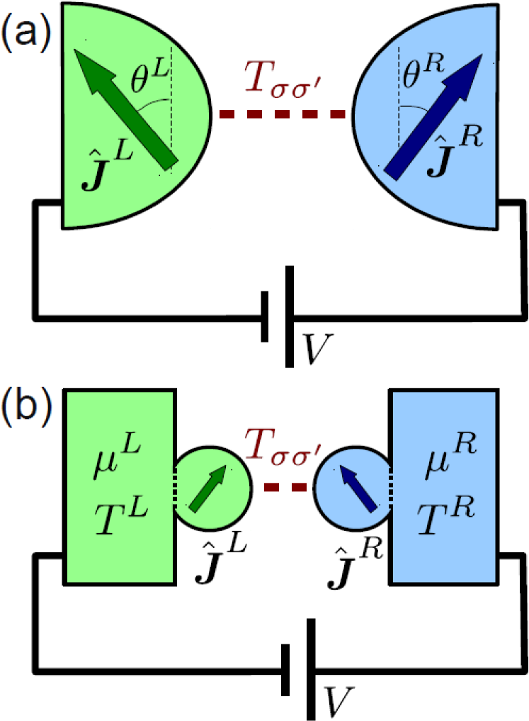
Figure 1: Spin-valve setup: a tunnel junction between  (a)  macroscopic ferromagnets with Stoner fields  $\mathbf{J}^{r}=J^{r}\widehat{\mathbf{J}}^{r}$. (b) mesoscopic islands with local magnetic fields $B^{r}=J^{r}\widehat{\mathbf{J}}^{r}$, each in equilibrium with energy- and particle- reservoir. A combination of (a) and (b) is another possibility (not shown).

We start from a quite general model Hamiltonian

$$H = H^{L}_{0}+H^{R}_{0}+H_{T}$$ (7)

with the non-interacting Hamiltonians of subsystem $r=L,R$:

$$H_{0}^{r} = \sum_{nk\sigma}\varepsilon_{nk\sigma}^{r}c^{{\dagger}}_{rnk\sigma}c_{rnk\sigma},$$ (8)

and the tunneling Hamiltonian with $T^{LR}_{\sigma\sigma^{\prime}}=(T^{RL}_{\sigma^{\prime}\sigma})^{\ast}$:

$$H_{T} =\sum_{nn^{\prime}kk^{\prime}\sigma\sigma^{\prime}}T^{LR}_{\sigma\sigma^{\prime}}c_{Lnk\sigma}^{{\dagger}}c_{Rnk^{\prime}\sigma^{\prime}}+\text{h.c.}$$ (9)

Here the field operators $c_{rnk\sigma}$ act on the single particle level $k$ of band $n$ in subsystem $r=L,R$ with spin $\sigma=\uparrow,\downarrow$. We assume that the single-electron spin $\mathbf{s}$ for every orbital $(n,k)$ in the same ferromagnet can be quantized along a common physical direction $\hat{\mathbf{J}}^{r}$ (with $|\hat{\mathbf{J}}^{r}|=1$), i. e.,

$$\left(\widehat{\mathbf{J}}^{r}\cdot\mathbf{s}\right)|\sigma\rangle_{r}=\sigma|\sigma\rangle_{r},$$ (10)

with $|\sigma\rangle_{r}=e^{-i\theta^{r}\hat{\mathbf{m}}\cdot\mathbf{s}}|\sigma\rangle_{\mathbf{e}_{z}}$ where we rotate by the angle $\theta^{r}$ between $\widehat{\mathbf{J}}^{r}$ and $\mathbf{e}_{z}$ about the axis perpendicular to both these vectors, defined by $\hat{\mathbf{m}}=\mathbf{e}_{z}\times\hat{\mathbf{J}}^{r}\text{/}|\mathbf{e}_{z}\times\hat{\mathbf{J}}^{r}|$ . For simplicity, we assume the tunneling amplitudes to be band- ($n$) and energy-($k$) independent; moreover, the spin is conserved by the tunneling, $\left[H_{T},\mathbf{S}\right]=0$. Nevertheless, the tunneling amplitudes in Eq. (9)

$$T^{LR}_{\sigma\sigma^{\prime}} = t{}\text{}_{L}\langle\sigma|\sigma^{\prime}\rangle_{R}$$ (11)

are in general spin-dependent because the field operators $c_{Lnk\sigma}$ and $c_{Rnk\sigma}$ annihilate electrons with spins quantized along non-collinear directions $\widehat{\mathbf{J}}^{L}\nparallel\widehat{\mathbf{J}}^{R}$. The spin conservation in the tunneling is reflected by a spin-independence of the “bare” tunneling amplitude $t$. More on this can be found in App. E, where we include spin-symmetry breaking tunneling processes in our extension of the real-time transport theory.

We model the two subsystems as reservoirs, each kept in a thermal equilibrium state $\rho^{r}=e^{-(H^{r}_{0}-\mu^{r}N^{r})/T^{r}}/Z_{r}$ where $Z^{r}=\text{Tr}e^{-(H^{r}_{0}-\mu^{r}N^{r})/T^{r}}$ is the grand-canonical partition function and $N^{r}$ is the particle number operator of electrode $r$. Both electrodes are have fixed electrochemical potentials $\mu^{r}$and temperatures $T^{r}$, whose gradients drive the stationary state currents of interest. Note that even if the tunneling is present, each electrode is held in equilibrium at each instant of time.

II.3 Two-Particle Density of States

In Sec. III we will calculate the expectation values of the charge and the spin multipoles involving sums over the mode index $k$. We now indicate which quantities parametrize the spin information from the ferromagnetic electrodes. As usual, we take the continuum limit and replace sums over $k$ by a frequency integral. For one-particle quantities such as charge and spin, one can expresses the results in terms of the spin-dependent one-particle density of states (1DOS):

$$\nu^{r}_{\sigma}(\omega) = \sum_{n,k}\delta(\varepsilon_{nk\sigma}^{r}-\omega)$$ (12)

$$= \bar{\nu}^{r}(\omega)(1+\sigma n^{r}(\omega)),$$ (13)

where $\bar{\nu}^{r}(\omega)$ is the spin-averaged DOS

$$\bar{\nu}^{r}(\omega) = \frac{\nu_{\uparrow}^{r}(\omega)+\nu_{\downarrow}^{r}(\omega)}{2}.$$ (14)

All the spin-dependence of the 1DOS is contained in the spin polarization (of the 1DOS)

$$n^{r}(\omega) = \frac{\nu_{\uparrow}^{r}(\omega)-\nu_{\downarrow}^{r}(\omega)}{\nu_{\uparrow}^{r}(\omega)+\nu_{\downarrow}^{r}(\omega)}.$$ (15)

Importantly, we will find that the 1DOS (13), although formulated for a general one-particle energy spectrum $\varepsilon^{r}_{nk\sigma}$, is not sufficient to quantify quantum transport of spin completely, in particular the spin-spin correlations described by the spin-quadrupole moment. We will see that the latter requires an additional, spin-dependent two-particle exchange DOS (2DOS):

$$\nu^{r}_{\sigma\sigma^{\prime}}(\omega,\omega^{\prime}) = \sum_{n,k}\delta(\varepsilon_{nk\sigma}^{r}-\omega)\delta(\varepsilon_{nk\sigma^{\prime}}^{r}-\omega^{\prime}).$$ (16)

The physical meaning of the 2DOS can be understood most easily by considering two identical copies of the same ferromagnet. The 2DOS is nonzero if there is a pair of states for an electron with spin $\sigma$ at energy $\omega$ in the first copy and an electron of spin $\sigma^{\prime}$ at energy $\omega^{\prime}$ in the second copy, but within the same $k$-mode in the same band $n$. We emphasize that the latter restriction requires additional modeling: one cannot make independent approximations for the 1DOS and the 2DOS since they are not completely independent of each other: for example, the spin-diagonal components of the 2DOS must satisfy the relation $\nu_{\sigma\sigma}^{r}(\omega,\omega^{\prime})=\delta(\omega-\omega^{\prime})\nu^{r}_{\sigma}(\omega)$. Yet, the remaining components of the 2DOS, $\nu_{\sigma\bar{\sigma}}(\omega,\omega^{\prime})$, where $\bar{\sigma}=-\sigma$ denotes the opposite of $\sigma$, can not be constructed from 1DOS. If the energies of electrons with spin $\sigma$ and $\bar{\sigma}$ are related by a function $\varepsilon^{r}_{nk\bar{\sigma}}=g^{r}_{n\sigma\bar{\sigma}}(\varepsilon^{r}_{nk\sigma})$ (for example, if the dispersion relation can be solved for $k$), then

$$\nu^{r}_{\sigma\sigma^{\prime}}(\omega,\omega^{\prime}) = \nu^{r}_{\sigma}(\omega)\delta(g^{r}_{n\sigma\sigma^{\prime}}(\omega)-\omega^{\prime})$$ (17)

with $g^{r}_{n\sigma\sigma}(\omega)=\omega$ trivially. Clearly, more than the 1DOS is needed here. As a consequence, in general one has to start from the spin dependent dispersion relation and calculate all required components of the 1- and 2DOS consistently. Transport of two-particle transport properties therefore probes more of the electronic structure of the ferromagnets than the one-particle currents of charge and spin.

II.4 Stoner Model and Flat Band Approximation

The central results of this paper, Eq. (96)-(98), are valid for general case of the above 1-DOS and 2DOS. However, since we focus on physically understanding spin-anisotropy transport, rather than making material-specific predictions, we keep all complications by band structure / dispersion relation features to a minimum.

Stoner model / external magnetic field. As explained above, we must specify the spin-dependence of the dispersion relation for a consistent treatment of the 1DOS and 2DOS. We model this by a rigid (i. e., energy-independent) splitting of absolute value $J^{r}_{n}$ between the spin $\uparrow$ and spin $\downarrow$ states,

$$\varepsilon^{r}_{nk\sigma} = \varepsilon^{r}_{nk}-\sigma J^{r}_{n}\text{/}2,$$ (18)

which may be different in each band $n$. This model can be used to discuss several situations, sketched in Fig. 1 (a)-(b). In case (a) macroscopic ferromagnets are treated within the Stoner model. In this case $J^{r}_{n}$ can differ depending on the strength of the electron-electron interaction in each band. In this case the restriction $J^{r}_{n}\gtrsim T^{r}$ must imposed to avoid the breakdown of ferromagnetism (which is not modeled by  Eq. (8)). In case (b) we consider mesoscopic magnetic islands, each in equilibrium with a reservoir. One may now let the $J^{r}_{n}$ model an external magnetic field, which may be different locally in each electrode, i.e., we identify $J^{r}_{n}=B^{r}$. The main difference between (a) and (b) is the relative importance of quantum exchange contributions in two-particle spin quantities due to the smaller magnetic moment of the reservoirs (see below). When considering nanoscopic islands charging and non-equilibrium effects on the transport will of course be important, which are neglected here. The main motivation for considering case (b) is that it provides an interesting comparison with results for quantum dot spin-valves where the latter effects are fully taken into account Sothmann and König (2010); Baumgärtel et al. (2011). For readability we will discuss the results throughout the paper in the language of case (a), ferromagnets with Stoner splittings, unless explicitly stated otherwise.

Flat Band Approximation. We secondly restrict ourselves to a single, flat band (sketched in Fig. 2) in each ferromagnet in the limit of large bandwidth $2D^{r}=2D$. The latter limit assumes that all other energy scales $(T^{r},J^{r},\mu^{r})$ are much smaller than the distance $W$ of the band edge closest to all electro-chemical potentials, given

$$W := \underset{r,r^{\prime},\sigma,p}{\min}\left(pD-\sigma\frac{J^{r}}{2}-\mu^{r^{\prime}}\right),$$ (19)

which is positive since we assume all $\mu^{r}$ to lie inside the bands. We refer to this in the following shortly as the flat band approximation, keeping in mind that we actually refer to a set of assumptions. For all frequencies $\omega<W$, the spin-dependent DOS is given by

$$\nu^{r}_{\uparrow}=\nu^{r}_{\downarrow} = \frac{N_{o}}{2D},$$ (20)

where $N_{o}$ is the total number of orbitals in each subsystem and

$$\nu_{\sigma\sigma^{\prime}}^{r}(\omega,\omega^{\prime}) = \nu_{\sigma}^{r}(\omega)\delta\left(\omega+\tfrac{\sigma-\sigma^{\prime}}{2}J-\omega^{\prime}\right),$$ (21)

where we used Eq. (18) to rewrite Eq. (17). One may criticize the simplicity of this approximation in that it does not account for spin-polarization near the Fermi energy, but only for a Stoner shift, which is only noticeable at the band edges. We will see in Sec. V.1, however, that this already captures plenty of important aspects in SQM transport.

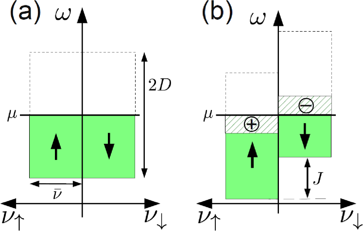
Figure 2: Spin-dependent density of states of a single flat band for a non-magnetic system (left) and a Stoner ferromagnet (right). The Stoner splitting redistributes a fraction of $J\text{/}4D$ of the $N_{o}$ particles from spin-down to the spin-up states relative to the non-magnetic case as indicated by the $+$ and $-$. We omit the electrode and band index for simplicity.

Clearly, the results for the average particle number, spin, SQM and their currents have to be independent of the choice of both the coordinate system and the spin-quantization axis (spin Hilbert space basis); they may only depend on the physical vectors $\hat{\mathbf{J}}^{r}$ and the scalar parameters $\mu^{r},T^{r}$ and $J^{r}_{n}$ and $t$ (below). A key technical result of the paper is that we reformulate real-time diagrammatic transport theory such the calculation is explicitly shows this covariance at every stage, which also makes it much more efficient (see  App. E).

Moreover, the usual modification that implements a spin-dependent DOS as $\nu_{\sigma}=\bar{\nu}(1+\sigma n)$ with constant $\bar{\nu}$ and $n$ is only valid as long one deals with single-particle observables such as the spin (even when accounting for many-body effects). For these calculations, all results can usually be expressed using the 1DOS. However, when dealing with two-particle observables relying on the 2DOS, it is crucial to specify the dispersion relation as we discussed in Sec. II.3. The above spin-dependent but constant DOS physically arises from mixing of different types orbitals in a tight-binding picture, resulting in more than one band. These additional bands can often be ignored, but this is no longer true for the 2DOS which is sensitive to these details. To make this clear, we merely mention two possible valid alternative models accounting consistently for a spin-polarization at the Fermi energy: (i) a single curved band (see Fig. 3 (a)) and (ii) two bands with different bandwidths and a large Stoner splitting so that different bands overlap at the Fermi energy (see Fig. 3 (b)). Since our single, flat wide band approximation is already sufficient to illustrate essential effects of spin-quadrupole storage and transport we will not pursue these band-structure details further here.

Figure 3: (a) Spin- and energy-dependent density of states for a one-band Stoner ferromagnet (b) Spin-dependent, constant density of states for a two-band Stoner ferromagnet with different bandwidths $2D_{n}$ and Stoner splittings $J_{n}$ for band $n=1,2$.

III Spin-Multipole Storage

In this section, we show that a system of ferromagnets, each kept at equilibrium, does not only store charge and spin polarization, but also stores spin anisotropy, quantified by the expectation value of the spin-quadrupole moment operator (1).

In Sec. III.1 we will first investigate the simplest case of a single ferromagnet at zero temperature. We discuss how the average SQM tensor relates to fluctuations in a macro-spin picture and relate this to the microscopic triplet spin-spin correlations. We identify an exchange contribution, which accounts for a “hole” in the quantum two-particle correlations of the spins due to the Pauli principle, giving rise to negative or Pauli-forbidden anisotropy.

In Sec. III.2 we extend these considerations to finite temperatures and multiple electrodes (without coupling them, i.e., $H_{T}=0$), both of which introduce new aspects. The case of two electrodes needs to be carefully addressed in order to define an SQM current later on: we must understand from where and to where SQM flows. It turns out that the ferromagnetic electrodes cannot simply be identified with the sources of SQM and we formalize our considerations in a convenient general spin-multipole network theory in Sec. III.2.2.

III.1 Single Electrode at $T=0$

We first calculate and analyse the average particle number, spin-dipole moment and spin-quadrupole moment of an isolated electrode in the simple limit of zero temperature in the approximation of a Stoner-shifted flat band (see II.4). In this subsection we will omit the electrode index $r$ and band index $n$ and denote by $\langle\text{ \ }\rangle=\langle\psi_{0}|\text{ \ }|\psi_{0}\rangle$ the $T=0$ ground state average.

III.1.1 Average Charge and Spin

We first review the average charge and spin-dipole moment for later comparison of these one-particle quantities with the SQM, a two-particle quantity. For zero temperature, all states with energy $\varepsilon_{k\sigma}\leqslant\mu$ below the electro-chemical potential $\mu$ are occupied and all levels with $\varepsilon_{k\sigma}>\mu$ are empty (cf. Fig. 2). Thus, the ground state average of particle number operator

$$N = \sum_{k,\sigma}c^{{\dagger}}_{k\sigma}c_{k\sigma},$$ (22)

corresponds to the sum of the green areas below the electro-chemical potential in Fig. 2: with $\nu_{\sigma}=\bar{\nu}$ we find

$$\langle N\rangle = \sum_{\sigma}\bar{\nu}\left(\mu+D+\frac{\sigma}{2}J\right)$$ (23)

$$= N_{o}\left(1+\frac{\mu}{D}\right).$$ (24)

Here $N_{o}=2D\bar{\nu}$ is the number of orbitals in the bandwidth $2D$. The particle number is independent of the Stoner splitting $J$ in this simple approximation.

The average of the spin operator,

$$\mathbf{S} = \sum_{k,\sigma}\mathbf{s}_{\sigma\sigma^{\prime}}c^{{\dagger}}_{k\sigma}c_{k\sigma^{\prime}},$$ (25)

measures the spin-dipolarization of the system, where $(s_{i})_{\sigma\sigma^{\prime}}=(\sigma_{i})_{\sigma\sigma^{\prime}}\text{/}2$ and $\sigma_{i}$,  $i=x,y,z$  are the Pauli matrices. Choosing the coordinate system such that $\mathbf{e}_{z}=\hat{\mathbf{J}}$, we obtain for $T=0$: $\langle S_{x}\rangle=\langle S_{y}\rangle=0$ and

$$\langle S_{z}\rangle = \tfrac{1}{2}\sum_{\sigma}\sigma\bar{\nu}\left[\mu-\left(-D-\frac{\sigma}{2}J\right)\right]=\tfrac{1}{2}N_{s}.$$ (26)

This equals the difference of the number of spin up and down electrons, i.e., the number of half-filled orbitals with polarized spins,

$$N_{s} = \bar{\nu}J=\frac{J}{2D}N_{o},$$ (27)

and corresponds to the difference of the areas under two DOS curves below $\mu$ in Fig. 2.

III.1.2 Average SQM and Spin Anisotropy

The average SQM $\langle\bm{\mathcal{Q}}\rangle=\sum_{ij}\langle Q_{ij}\rangle\mathbf{e}_{i}\mathbf{e}_{j}$ is a real and symmetric tensor, which can therefore always be diagonalized. With the above choice of the coordinate system with $\mathbf{e}_{z}=\hat{\mathbf{J}}$, $\langle Q_{ij}\rangle$ is already diagonal by symmetry with respect to rotations about $\hat{\mathbf{J}}$. The average of the non-zero tensor operator component

$$Q_{zz} = \tfrac{2}{3}S_{z}^{2}-\tfrac{1}{3}(S^{2}_{x}+S^{2}_{y})$$ (28)

now measures the spin anisotropy with respect to the $z$-axis in the ground state:  $\langle Q_{zz}\rangle>0$ indicates that the spin is aligned (but not necessarily oriented) with the easy $z$-axis, while $\langle Q_{zz}\rangle<0$ indicates an easy-plane configuration where the spin preferably lies in the perpendicular $xy$-plane. If $\langle Q_{zz}\rangle$ vanishes, neither alignment longitudinal or transverse to the $z$-direction is favoured. This is the case, e.g., for a spin-isotropic state for which $\langle S_{x}^{2}\rangle=\langle S_{y}^{2}\rangle=\langle S_{z}^{2}\rangle$; however, it can also be realized by states that are anisotropic in $xy$-plane, for which $\langle S_{x}^{2}\rangle\neq\langle S_{y}^{2}\rangle$ while $\langle S_{z}^{2}\rangle=\frac{1}{2}\left(\langle S_{x}^{2}\rangle+\langle S_{y}^{2}\rangle\right)$. These two situations are thus distinguished by the average of one other non-zero SQM tensor components $\langle Q_{xx}\rangle$ or $\langle Q_{yy}\rangle$ (since $\sum_{i}\langle Q_{ii}\rangle=0$ these are not independent).

We now investigate to what extent the average spin polarization in a Stoner ferromagnet implies a uniaxial anisotropy. Classically, one expects spin polarization to always imply some nonzero spin anisotropy, but the converse need not be true as our example in Sec. I showed. We now calculate the average SQM in two ways, first focusing an a collective macrospin picture, common in atomic and molecular magnetism, and then disentangling it into its microscopic contributions from electron pairs relevant to spintronics.

Average Macrospin SQM

The ground state of the ferromagnet is a maximally polarized pure spin state,  $|\psi_{0}\rangle=|S,m=S\rangle$(as sketched in Fig. 4).

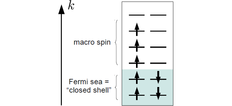
Figure 4: Schematics of the occupation of the orbitals for an electrode at zero temperature: doubly occupied orbitals form a zero spin state (Pauli principle) while all spins in the singly occupied orbitals are parallel, maximizing the total spin (c. f. text)

The value of the spin $S$ is determined from the half-filled orbitals with $N_{s}$ polarized spins

$$\begin{array}[]{lllll}S&=&\langle S_{z}\rangle&\approx&\tfrac{1}{2}N_{s}\end{array}.$$ (29)

Since $|\psi_{0}\rangle$ is a maximal spin eigenstate there are no quantum fluctuations in the first, longitudinal part of Eq. (28): $\langle S_{z}^{2}\rangle=\langle S_{z}\rangle^{2}$. The second, transverse contribution, however, can be written as $S^{2}_{x}+S^{2}_{y}=S_{-}S_{+}-i[S_{x},S_{y}]=S_{-}S_{+}+S_{z}$ using $S_{\pm}=S_{x}\pm iS_{y}$. It has a non-vanishing part due to the quantum spin commutation relations: since $S_{+}|\psi_{0}\rangle=0$, $\langle S^{2}_{x}+S^{2}_{y}\rangle=\langle S_{z}\rangle$. The $T=0$ average Eq. (28) is found to be

$$\langle Q_{zz}\rangle = \tfrac{2}{3}\langle S_{z}^{2}\rangle-\tfrac{1}{3}\langle S^{2}_{x}+S^{2}_{y}\rangle$$ (30)

$$= \tfrac{2}{3}S^{2}-\tfrac{1}{3}S,$$ (31)

The spin-anisotropy, quantified by the average SQM, thus has competing contributions: spin-polarization induces anisotropy in the $z$-direction ($\propto S^{2}$), but transverse spin fluctuations tend to suppress it ($\propto S$). The quantum fluctuations of the spin  in the ground state “resist” perfect alignment of the spin, despite the maximal spin alignment. In fact, Eq. (31) also holds with $N_{s}=1$, $S=1/2$ in which case the longitudinal term is completely cancelled by the transverse fluctuations: a spin 1/2 is “so quantum” that it always has zero spin anisotropy due to spin fluctuations, in fact, in any state. Since the filled shells do not contribute to the value of $S$, this suggests that $\langle Q_{zz}\rangle$ at $T=0$ only accounts for triplet correlations between the open shell electrons with parallel spin. However, a full understanding of the transverse fluctuations needs a further refinement of that picture.

Microscopic SQM Storage

Above we linked the zero-temperature average SQM to the spin anisotropy stored in a ferromagnet and related it to its average collective spin and its transverse quantum fluctuations. We will investigate now how these quantum fluctuations tend to smear out the spin, reducing the uniaxial anisotropy. For this, we decompose the spin anisotropy into its microscopic contributions from all particles: we start with the longitudinal contribution to $Q_{zz}$ in Eq. (28) and express the total spin operator $S_{z}=\sum_{a}s_{z}^{a}$ as the sum of the single- electron spins:

$$S_{z}^{2}=\sum_{a}(s_{z}^{a})^{2}+2\sum_{a<b}s_{z}^{a}s_{z}^{b}$$ (32)

$$=\sum_{k\sigma}\tfrac{1}{4}c^{{\dagger}}_{k\sigma}c_{k\sigma}+\sum_{kk^{\prime}\sigma\sigma^{\prime}}\tfrac{\sigma\sigma^{\prime}}{4}c^{{\dagger}}_{k\sigma}c^{{\dagger}}_{k^{\prime}\sigma^{\prime}}c_{k^{\prime}\sigma^{\prime}}c_{k\sigma}.$$ (33)

Thus, $S_{z}^{2}$ has both a one- and a two-electron part. When averaging, the first term gives $\sum_{\sigma}\tfrac{1}{4}N_{\sigma}$ where $N_{\sigma}=(D+\sigma J)\text{/}2$ is the number of orbitals occupied with spin $\sigma$. For the two-particle part, we can first treat the electrons as if they were classically distinguishable, yielding a contribution whenever the states $(k,\sigma)$ and $(k^{\prime},\sigma^{\prime})$ are occupied. This allows us to factorize the resulting expression $\left(\sum_{\sigma}\tfrac{\sigma}{2}N_{\sigma}\right)\left(\sum_{\sigma^{\prime}}\tfrac{\sigma^{\prime}}{2}N_{\sigma^{\prime}}\right)=\tfrac{1}{4}N_{s}^{2}$ into the product of averages, i. e., $\langle S_{z}\rangle^{2}$ . We therefore call this a direct (two-particle) contribution. However, if $(k,\sigma)=(k^{\prime},\sigma^{\prime})$, we have to be careful: due to Pauli’s principle, it is forbidden to annihilate electrons in the same state twice, hence we have to exclude this possibility by a correction term $-\sum_{\sigma}\tfrac{\sigma\sigma}{4}N_{\sigma}=-N_{o}$. We call this the exchange (two-particle) contribution, a denotation that will become more clear in III.2.3. This yields altogether

$$\langle S^{2}_{z}\rangle = \tfrac{1}{4}(N_{o}+N_{s}^{2}-N_{o})=\langle S_{z}\rangle^{2},$$ (34)

confirming the result trivially obtained in the macrospin picture (since $|\psi_{0}\rangle$ is an eigenstate of $S_{z}$). The classical intuition is only correct because of a non-trivial cancellation of a one-particle and “quantum” Pauli-exclusion term on a microscopic level. This importance of this subtlety will become clear later (cf. Sec. III.2.4).

We proceed with decomposing the transverse fluctuations into a one-particle and a two-particle term,

$$S_{x}^{2}+S_{y}^{2}=\sum_{i=x,y}\left[\sum_{a}(s_{i}^{a})^{2}+2\sum_{a<b}s_{i}^{a}s_{i}^{b}\right]$$ (35)

$$=\sum_{k\sigma}\tfrac{1}{2}c^{{\dagger}}_{k\sigma}c_{k\sigma}+\sum_{kk^{\prime}\sigma\sigma^{\prime}}\tfrac{1-\sigma\sigma^{\prime}}{4}c^{{\dagger}}_{k\bar{\sigma}}c^{{\dagger}}_{k^{\prime}\bar{\sigma}^{\prime}}c_{k^{\prime}\sigma^{\prime}}c_{k\sigma},$$ (36)

and averaging over the ground state yields a non-vanishing one-particle term $\tfrac{1}{2}\sum_{\sigma}N_{\sigma}$, describing transverse single-spin fluctuations. For the two-particle part, the direct term vanishes as the individual spins are flipped in the modes $k$ and $k^{\prime}$ so that the ground state is not reproduced any more. This agrees with the fact that the averages $\langle S_{x}\rangle=\langle S_{y}\rangle=0$. However, we must again treat the case $k=k^{\prime}$ separately: when this mode is doubly occupied and we have $\sigma^{\prime}=\bar{\sigma}$, the sequence of the four field operators together exchanges the spins, reproducing the ground state. This gives a correction $-N_{\downarrow}$, which is again due to Pauli’s principle: a configuration of two indistinguishable spins and the same configuration with both spin exchanged cannot be told apart. This two-electron exchange fluctuations together with the single-spin fluctuations make up for the total transverse fluctuations of the macrospin,

$$\begin{array}[]{lllll}\langle S^{2}_{x}+S^{2}_{y}\rangle&=&\tfrac{1}{2}N_{o}-N_{\downarrow}&=&\langle S_{z}\rangle\end{array}.$$ (38)

If we we next combine the longitudinal and the transverse term to obtain $\langle Q_{zz}\rangle$, we see that the one-particle contributions drop out:

$$\langle Q_{zz}\rangle = \tfrac{1}{6}N_{s}^{2}-\left(\tfrac{1}{6}N_{o}+\tfrac{1}{3}N_{\downarrow}\right).$$ (39)

As the SQM of a spin-1/2 vanishes (cf. the end of Sect. III.1.2), the SQM exclusively measures true two-spin correlations and does not contain any single-spin information: The second bracket in Eq. (39) is a pure two-spin exchange correction that accounts a kind of “hole” in the triplet correlations. The notion of this “Pauli exclusion hole” will be explained prescisely in Sec. III.2.4. It physically arises from exchange contributions both in $\langle S^{2}_{z}\rangle$ and $\langle S^{2}_{x}+S^{2}_{y}\rangle$. Eq. (39) can be expressed as

$$\langle Q_{zz}\rangle = \tfrac{1}{3}\times\tfrac{1}{2}N_{s}(N_{s}-1).$$ (40)

Thus, in the present case, the SQM counts the number of pairs of the parallel spins in different half-filled orbitals. In accordance with the macrospin picture, the doubly occupied orbitals can be simply ignored. However, at finite temperatures, the Fermi edge becomes unsharp and modes below the the electro-chemical potential $\mu$ also contribute to SQM. In contrast to the macrospin picture, the present microscopic description already included the entire Fermi sea into the description and can therefore be extended to finite temperatures (see Sect. III.2.4). For $T>0$ we will also directly start from $\bm{\mathcal{Q}}$ in second-quantized from, which provides a clear way to demonstrate why SQM only senses spin-triplet correlations.

Importantly, these direct and exchange contribution to Eq. (39) scale differently with the number of polarized spins $N_{s}=\frac{J}{2D}N_{o}$. For a macroscopic ferromagnet, the exchange contribution to the SQM can be be neglected due to the relative unimportance of excluding a single orbital among many. In this case, SQM is entirely induced by spin-dipolarization. For $N_{s}\rightarrow\infty$ the SQM per pair of polarized spins has only a finite direct contribution of $1/3$ by Eq. (40), or alternatively, per orbital $(J\text{/}2D)^{2}\text{/}3$. For mesoscopic ferromagnetic systems with $N_{s}\sim 10-100$ polarized spins the exchange corrections start to become relevant, and for magnetic molecular quantum dots in magnetic field $N_{s}\sim 1-10$ and both terms can even be of comparable size. In both these cases, the exclusion principle for a few quantum levels becomes relatively important.

III.2 Two Electrodes at $T>0$

We now extend the above analysis to two electrodes, which are, moreover, at finite temperatures $T^{L}$ and $T^{R}$. This brings in two new aspects. First, in Sec. III.2.1, we find that for finite temperatures that the average SQM cannot be expressed anymore in the average spin as for $T=0$. The exchange SQM contribution is responsible for this difference, quantifying pure quantum contributions to the anisotropy as we will see in Sec. III.2.3. This contribution involves a  two-particle exchange DOS, which is evaluated and discussed in Sec. III.2.4. This new quantity is used to explain the notion of a “Pauli exclusion hole” in the triplet spin correlations, which are encoded in the SQM. This provides the key to understanding how quantum two-particle exchange processes allow for an SQM current in the absence of spin-dipole current, the central result of the paper in Sec. V.3.

The second new aspect, the subdivision of the system into smaller units, touches upon the seemingly naive question of how to define an SQM current. Clearly, an SQM current cannot quantify the “amount” of spin anisotropy that flows through a tunnel barrier as single tunneling electrons have zero SQM: this idea only makes sense for a one-particle quantity such as charge or spin. In contrast, SQM is a two-particle quantity, i. e., built up by pairs of electrons. As the electrons of a pair can stay at different sides of the tunnel junction, SQM is not only stored locally in each ferromagnet, but also non-locally between the ferromagnets. The concept of storage of SQM thus needs to include nonlocal sources of SQM in addition to the local ones discussed so far. In Sec. III.2.2 we develop a spin-multipole network theory to aid the physical intuition and which will prove to be very helpful  for the discussion of SQM transport later on and which has a wider range of application than the model studied in this paper.

III.2.1 Average Charge and Spin

In the following we calculate the average charge and spin-dipole moment in a more technical way and in some more detail. We illustrate how to rewrite the spin-dependent part of expectation values most elegantly in terms of expressions independent of the choice of the coordinate system and of the spin quantization axis. This serves as a good example of the manipulations we present in App. E where we reformulate the real time diagrammatic transport theory in an explicitly covariant way. Firstly, the one-particle operators (22) for the charge  and (25) for the spin (now including the reservoir index $r$) are jointly described by the four-component operator

$$R_{\mu}^{r} = \sum_{k,\sigma,\sigma^{\prime}}(r^{r}_{\mu})_{\sigma\sigma^{\prime}}c^{{\dagger}}_{rk\sigma}c_{rk\sigma^{\prime}}.$$ (41)

Here $(r^{r}_{\mu})_{\sigma\sigma^{\prime}}=\text{}_{r}\langle\sigma|r_{\mu}|\sigma^{\prime}\rangle_{r}$ denotes the matrix elements of the single-particle operator $r_{\mu}$ for spin states quantized along $\hat{\mathbf{J}}^{r}$. Using $r_{0}=\mathbbm{1}$ and $r_{i}=s_{i}$ ensures that $R_{0}=N$ and $R_{i}=S_{i}$ for $i=1,2,3$. We will from hereon distinguish whether the 0-component is included or not by using Greek or Latin indices, respectively. Taking the average of Eq. (41) involves

$$\langle c_{rk\sigma}^{{\dagger}}c_{r^{\prime}k^{\prime}\sigma^{\prime}}\rangle = f^{r}_{+}(\varepsilon^{r}_{k\sigma})\delta_{rr^{\prime}}\delta_{kk^{\prime}}\delta_{\sigma\sigma^{\prime}}$$ (42)

with the Fermi function

$$f^{r}_{+}(\omega) = \frac{1}{e^{(\omega-\mu^{r})/T^{r}}+1}.$$ (43)

Recasting the sum over all $k$-modes as an integral over all energies by inserting the DOS (see Eq. (13)) yields

$$\langle R_{\mu}^{r}\rangle = \sum_{\sigma,\sigma^{\prime}}(r^{r}_{\mu})_{\sigma\sigma^{\prime}}\int\mathrm{d}\omega\delta_{\sigma\sigma^{\prime}}\nu_{\sigma}f^{r}_{+},$$ (44)

where we suppressed the $\omega$-dependence for brevity. Using Eq. (10), i. e. $\left(\mathbf{J}^{r}\cdot\mathbf{s}\right)|\sigma\rangle_{r}=\sigma|\sigma\rangle_{r}$, we may rewrite

$$\nu^{r}_{\sigma}(\omega)\delta_{\sigma\sigma^{\prime}} = \bar{\nu}^{r}(\omega)\text{}_{r}\langle\sigma|\check{\mathbf{n}}^{r}(\omega)\cdot\check{\mathbf{r}}|\sigma^{\prime}\rangle_{r},$$ (45)

introducing $\check{r}_{0}=\mathbbm{1}\text{/}\sqrt{2}$ and $\check{\mathbf{r}}=\sqrt{2}\mathbf{s}$  and the four-component vector $\widehat{\mathbf{n}}^{r}=\sqrt{2}(1,\widehat{\mathbf{J}}^{r}n^{r})$. The spin-dependent part of Eq. (44) can be recast as a trace in spin space:

$$\left\langle\mathbf{R}^{r}\right\rangle = \int\mathrm{d}\omega\bar{\nu}^{r}f^{r}_{+}\text{Tr}\left[\mathbf{r}\left(\check{\mathbf{n}}^{r}\cdot\check{\mathbf{r}}\right)\right].$$ (46)

The trace is clearly covariant in the general sense, i.e., form-invariant under changes of either the coordinate system and / or quantization axis (it is not related to concepts from relativity; vectors with four elements are just convenient). We obtain

$$\langle N^{r}\rangle = \int d\omega 2\bar{\nu}^{r}(\omega)f^{r}_{+}(\omega),$$ (47)

$$\langle\mathbf{S}^{r}\rangle = \int d\omega 2\bar{\nu}^{r}(\omega)s^{r}(\omega)\widehat{\mathbf{J}}^{r},$$ (48)

Analogous to the average occupation number of a single level at energy $\omega$ in (47), $f^{r}_{+}(\omega)$, we denote

$$s^{r}(\omega) = f^{r}_{+}(\omega)\tfrac{1}{2}n^{r}(\omega)$$ (49)

in Eq. (48) as the average spin-polarization function of electrons at frequency $\omega$, where $n^{r}(\omega)$ is the spin-polarization (15). Note that we only needs to use spin 1/2 operator algebra to calculate the average in Eq. (46) in coordinate-free form and the same can be done for all the less transport calculations, see App. E.

III.2.2 Network Picture: Non-Locality

Eqs. (47) and (48) show that each physical electrode  corresponds to a single source of charge and spin. We now formalize the concept of particle and spin-dipole storage  in terms of a network theory, which at first sight may seem superfluous. In fact, it will prove to be helpful to compare this with the storage and transport of spin-quadrupole moment.

The following considerations are formulated more compactly and hold more generally for a composite system of any number of subsystems labeled by an index $r$. Such a system may comprise of just two electrodes, each at equilibrium, as discussed in this paper (then $r=L,R$), but it may also include, e.g., strongly interacting quantum dots out of equilibrium as discussed in Sothmann and König (2010); Baumgärtel et al. (2011); Misiorny et al. (2012a) and in forthcoming works. We first ask how the total charge and spin-dipole moment is distributed over the subsystems. The answer is fairly intuitive for these one-particle quantities: the total charge (spin) is the sum of the charge (spin) stored in each electrode, i. e.,

$$R^{\mathrm{tot}}_{\mu} = \sum_{r}R^{r}_{\mu}.$$ (50)

We can simply associate each subsystem shown in Fig. 5 (a) with a node of charge (spin) as depicted in Fig. 5 (b). Note that decomposition (50) is even possible if $R^{\mathrm{tot}}_{\mu}$ is not conserved. (We postpone the discussion of the links in the network until we defined current operators in Sec IV where we complete the network theory.)

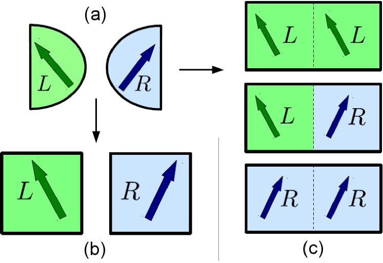
Figure 5: (a) Physical setup of two ferromagnets and network picture for (b) the spin-dipole moment, a one-particle quantity (like the charge) and for (c) the spin-quadrupole moment, a two-particle quantity.

This simple correspondence breaks down for SQM. When we ask how this two-particle quantity is distributed over composite system, the answer is radically different. We start from the total SQM of the system, written as

$$\bm{\mathcal{Q}}^{\mathrm{tot}} = \mathbf{S}^{\mathrm{tot}}\odot\mathbf{S}^{\mathrm{tot}}$$ (51)

abbreviating the symmetric, traceless dyadic product of two vector operators $\mathbf{a}$ and $\mathbf{b}$ as

$$\left(\mathbf{a}\odot\mathbf{b}\right)_{ij} = \tfrac{1}{2}(a_{i}b_{j}+b_{i}a_{j})-\tfrac{1}{3}\delta_{ij}\mathbf{a}\cdot\mathbf{b}$$ (52)

We decompose $\bm{\mathcal{Q}}^{\mathrm{tot}}$ by inserting $\mathbf{S}^{\mathrm{tot}}=\sum_{r}\mathbf{S}^{r}$,

$$\bm{\mathcal{Q}}^{\mathrm{tot}} = \sum_{\langle rr^{\prime}\rangle}\bm{\mathcal{Q}}^{rr^{\prime}},$$ (53)

where $\langle rr^{\prime}\rangle$ indicates that we sum only over all pairs

$$\begin{array}[]{lllll}\bm{\mathcal{Q}}^{rr^{\prime}}&=&\bm{\mathcal{Q}}^{r^{\prime}r}&=&g^{rr^{\prime}}\mathbf{S}^{r}\odot\mathbf{S}^{r^{\prime}},\end{array}$$ (55)

and the factor $g^{rr}=1$ and $g^{rr^{\prime}}=2$ ($r\neq r^{\prime}$) accounts for the double occurrence of each pair $r,r^{\prime}$ with $r\neq r^{\prime}$ in the expansion (51). Eq. (55) is symmetric in $r$ and $r^{\prime}$ since  $\mathbf{S}^{r}\odot\mathbf{S}^{r^{\prime}}=\mathbf{S}^{r^{\prime}}\odot\mathbf{S}^{r}$ and we can write

$$\bm{\mathcal{Q}}^{rr^{\prime}} = \tfrac{1}{2}g^{rr^{\prime}}(\mathbf{S}^{r}\odot\mathbf{S}^{r^{\prime}}+\mathbf{S}^{r^{\prime}}\odot\mathbf{S}^{r}).$$ (56)

Note that $\bm{\mathcal{Q}}^{rr^{\prime}}$ is a Hermitian operator and therefore an observable because spin operators of different subsystems commute: $(\mathbf{S}^{r}\odot\mathbf{S}^{r^{\prime}})^{{\dagger}}=\mathbf{S}^{r^{\prime}}\odot\mathbf{S}^{r}=\mathbf{S}^{r}\odot\mathbf{S}^{r^{\prime}}$.

We now develop a network picture for the SQM by associating to each pair of subsystems $\langle rr^{\prime}\rangle$ a single effective source or node. For the two-terminal spin-valve in Fig. 5(a) that we study, three SQM-nodes appear in the corresponding network picture of Fig. 5 (c). The total SQM is stored in two local nodes ($\bm{\mathcal{Q}}^{LL}$, $\bm{\mathcal{Q}}^{RR}$) and in one non-local node ($\bm{\mathcal{Q}}^{LR}=\bm{\mathcal{Q}}^{RL}$). The (non)local nodes describe spin-triplet correlations between pairs of electrons of the same (different) subsystem(s). This non-locality of SQM storage is very important for the physical understanding and definition of a SQM current operator. It is the injection of SQM currents from these non-local nodes that drive the measurable local SQM dynamics in embedded quantum dots, as found in Ref. Baumgärtel et al. (2011). For the spin-valve considered here it now becomes clear how single electron tunneling can transport SQM: first, local correlations, e. g., in the $\langle LL\rangle$-node are turned into non-local correlations in the $\langle LR\rangle$-node. The transfer of SQM is then completed by another single-electron tunneling event that re-localizes the pair, but now in the right electrode, contributing then to the $\langle RR\rangle$-node. This picture will be refined once we defined SQM current operators in Sec. IV.2.

III.2.3 Direct and Exchange Contribution to Average SQM

We next inquire to which extent the stored SQM is independent of the average spin-dipole moment, extending the discussion of Sec. III.1.2. The average of the SQM operator for node $\langle rr^{\prime}\rangle$ given by (55), can be decomposed it into a direct and an exchange part using Wick’s theorem for the averages of products of field operators (see App. A.3 for details):

$$\begin{array}[]{lll}\langle\bm{\mathcal{Q}}^{rr^{\prime}}\rangle&=&\langle\bm{\mathcal{Q}}^{rr^{\prime}}\rangle_{\mathrm{dir}}+\langle\bm{\mathcal{Q}}^{rr^{\prime}}\rangle_{\mathrm{ex}}\end{array}.$$ (57)

Direct SQM.  The first possible direct contraction combines field operators from the same spin operator in Eq. (30). It can therefore be factorized into the expectation values of the spin operators given by Eq. (48):

$$\langle\bm{\mathcal{Q}}^{rr^{\prime}}\rangle_{\mathrm{dir}} = \sum_{kk^{\prime}\sigma\sigma^{\prime}}\mathbf{s}^{r}_{\sigma\sigma}\odot\mathbf{s}^{r^{\prime}}_{\sigma^{\prime}\sigma^{\prime}}f_{+}^{r}(\varepsilon^{r}_{k\sigma})f^{r^{\prime}}_{+}(\varepsilon^{r^{\prime}}_{k^{\prime}\sigma^{\prime}})$$ (58)

$$= \langle\mathbf{S}^{r}\rangle\odot\langle\mathbf{S}^{r^{\prime}}\rangle=q^{rr^{\prime}}_{\text{dir}}\widehat{\mathbf{J}}^{r}\odot\widehat{\mathbf{J}}^{r^{\prime}}$$ (59)

with

$$q_{\text{dir}}^{rr^{\prime}} = |\langle\mathbf{S}^{r}\rangle|\,|\langle\mathbf{S}^{r^{\prime}}\rangle|.$$ (60)

This direct SQM incorporates the cumulative effect of the energy resolved spin-polarization $s^{r}(\omega)$. It quantifies the uncorrelated contribution of the quantum spins to the spin anisotropy: as intuitively expected, an electrode with a favoured spin direction (polarization) possesses a favoured spin alignment (anisotropy). For a macroscopic system in equilibrium, the average SQM is dominated by the direct part, which is completely determined by the average spin-dipole moment.

Exchange SQM. For meso- and  nanoscopic systems the last statement ceases to be true due to the neglect of the Pauli’s principle in the spin-spin correlations. In the second exchange contraction field operators of different spin operators are contracted, giving a term

$$\langle\bm{\mathcal{Q}}^{rr^{\prime}}\rangle_{\mathrm{ex}} = \delta^{rr^{\prime}}\sum_{k\sigma\sigma^{\prime}}\mathbf{s}^{r}_{\sigma\sigma^{\prime}}\odot\mathbf{s}^{r^{\prime}}_{\sigma^{\prime}\sigma}f_{+}^{r}(\varepsilon^{r}_{k\sigma})f^{r}_{+}(\varepsilon^{r}_{k\sigma^{\prime}}),$$ (61)

which accounts for true correlations in the sense of Spearman’s rank correlation coefficient. This becomes clear when rewriting Eq. (61) using Eq. (59):

$$\langle\bm{\mathcal{Q}}^{rr^{\prime}}\rangle_{\mathrm{ex}} = \mathbf{}\langle\mathbf{S}^{r}-\langle\mathbf{S}^{r}\rangle\rangle\odot\mathbf{}\langle\mathbf{S}^{r^{\prime}}-\langle\mathbf{S}^{r^{\prime}}\rangle\rangle.$$ (62)

Note that Eq. (61) involves only one sum over $k$. Thus, the exchange term indeed scales linearly with the system size in contrast to the direct term (see Eq. (59)) and can be neglected for macroscopic systems (cf. last paragraph in Sect. III.1.2). Here it is interesting to consider our Hamiltonian as a model for a mesoscopic ferromagnet or a metallic island in a strong external magnetic field, Fig. 1(b). In this case the exchange contribution may even become the dominant part in transport when the spin current vanishes: then the spin-polarization $\langle\mathbf{S}^{r}\rangle$ and therefore also $\langle\bm{\mathcal{Q}}^{rr^{\prime}}\rangle_{\mathrm{dir}}$ do not change, while $\langle\bm{\mathcal{Q}}^{rr^{\prime}}\rangle_{\mathrm{ex}}$ does. When including a tunnel-coupling between the ferromagnets the transport through the junction correlates spins of both systems and non-local exchange SQM currents can indeed arise. For this reason, we keep the exchange term here and study it in some more detail.

Tensorial structure. Eq. (62) can be expressed as

$$\langle\bm{\mathcal{Q}}\rangle_{\mathrm{ex}} = -\delta^{rr^{\prime}}q^{rr}_{\mathrm{ex}}\widehat{\mathbf{J}}^{r}\odot\widehat{\mathbf{J}}^{r}$$ (63)

with the positive quantity

$$q_{\mathrm{ex}}^{rr} = \tfrac{1}{4}\sum_{k}(f_{+}^{r}(\varepsilon^{r}_{k\uparrow})-f_{+}^{r}(\varepsilon^{r}_{k\downarrow}))^{2}>0.$$ (64)

(see App. A.2). Clearly, only if $\varepsilon_{k\uparrow}-\varepsilon_{k\downarrow}\ll T$ for all $k$, the exchange contribution vanishes, i.e., for the Stoner model if $J\ll T$. However, if $J<T$, each spin-polarized orbital $k$ gives a negative correction to the direct spin anisotropy. We will refer to this as the Pauli exclusion hole, located in orbital $k$ with a “distribution function” $(f(\varepsilon_{k\uparrow})-f(\varepsilon_{k\downarrow}))^{2}$. We give a microcopic interpetation of this below in Sec. III.2.4. A gradient of these Pauli exclusion holes across the junction results drives an exchange SQM current, which may even flow in the absence of a spin current, see Sec. V.3.

We moreover note that the tensor $\langle\bm{\mathcal{Q}}\rangle_{\mathrm{ex}}$ has the same principal axes as $\langle\bm{\mathcal{Q}}\rangle_{\text{dir}}$ (the reason for this is discussed in the following section). Thus, the local SQM $\left\langle\bm{\mathcal{Q}}^{rr}\right\rangle\propto\widehat{\mathbf{J}}^{r}\odot\widehat{\mathbf{J}}^{r}$, has a diagonal representation in any coordinate system that includes the Stoner field direction, e.g., $\mathbf{e}_{z}=\widehat{\mathbf{J}}^{r}$, with non-zero elements $\langle Q^{rr}_{xx}\rangle=\langle Q^{rr}_{yy}\rangle=-\langle Q^{rr}_{zz}\rangle\text{/}2$. This shows that the local SQM sources are uniaxially anisotropic, and different alignments in the plane perpendicular to $\hat{\mathbf{J}}^{r}$ are not preferred. Since the direct contribution exceeds the exchange contributions, we find as expected$\langle Q^{rr}_{zz}\rangle>0$, i.e., an easy-axis anisotropy favoring the collinear orientation of the spins into the $z$-direction over any orientation in the $xy$-plane, $\langle Q^{rr}_{xx}\rangle=\langle Q^{rr}_{yy}\rangle<0$.

The non-local SQM $\langle\bm{\mathcal{Q}}^{rr^{\prime}}\rangle$, $r\neq r^{\prime}$, has three non-degenerate principal values: it describes bi-axial anisotropy. It has a unique principal axes in which $\langle Q^{rr}_{zz}\rangle>\langle Q^{rr}_{yy}\rangle>\langle Q^{rr}_{xx}\rangle$, i.e., directions perpendicular to the dominant easy axis ($z$) are distinguished, see App. B.

III.2.4 Microscopic Picture of SQM Storage

The physical meaning of the exchange SQM becomes transparent when revisiting the microscopic picture of SQM storage. When calculating the direct SQM by Eq. (58) one pretends to have to two distinct ferromagnets $r$ and $r^{\prime}$ and “counts” triplet correlations by adding all cross-correlations between electrons occupying these distinguishable ferromagnets. This procedure gives the full result for the non-local SQM (cf. Eq. (61)): for $r\neq r^{\prime}$

$$\langle\bm{\mathcal{Q}}^{rr^{\prime}}\rangle = \langle\bm{\mathcal{Q}}^{rr^{\prime}}\rangle_{\mathrm{dir}}.$$ (65)

This is correct as we we treat the two ferromagnets as distinguishable objects by assumption (the total density operator is a direct product).

The direct, local SQM $(r=r^{\prime})$ also correctly “counts” the local spin anisotropy as long as it concerns correlations of electrons from different modes $k\neq k^{\prime}$, which are also distinguishable (green lines in Fig. 6). However, this procedure fails for electrons occupying the same mode $k^{\prime}=k$: a single mode (irrespective of whether being singly or doubly occupied) does not contribute to the total SQM (see App. A.3). Thus, the local exchange SQM has to cancel the contribution that the direct SQM  (58)  incorrectly ascribes to single modes (indicated by the red line in Fig. 6)

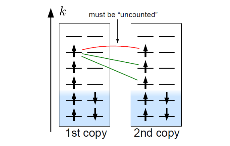
Figure 6: Microscopic contributions to the local SQM $\langle\bm{\mathcal{Q}}^{rr}\rangle$. Two copies of the same ferromagnet are considered and green lines indicate correlations between pairs of distinguishable electrons in different orbitals (counted by the direct SQM). The red line indicates the correlations between indistinguishable electrons in the same orbital that the direct SQM counts too much: according to Pauli’s principle two electrons cannot form a triplet state in the same orbital. The exchange SQM contribution takes care of this and thus represents a Pauli hole in the correlations, corresponding to the red line. When considering only the 1st copy at finite temperature, the macrospin picture discussed in Sect. III.1.2 is recovered. For finite temperature, the occupation probabilities are  thermally smeared at the Fermi edge.

For establishing an “uncounting” procedure to exclude the single-mode SQM, one may again simply think of two identical, but distinguishable copies of the same mode $k$ and calculate the direct SQM generated from all these modes (see Fig. 6). In this picture, exchange SQM represents a “spin-anisotropy hole” ascribed to each mode and therefore shows a formal analogy to a one-particle quantity. This analogy will reemerge when we consider the transport of SQM in Sect. III.2.5. To emphasize this multi-particle exchange aspect, we will refer to this as a Pauli exclusion hole in the spin triplet correlations.

As a consequence, local exchange SQM must have the same tensorial structure as the direct SQM, but with opposite magnitude, which is explicitly conveyed by the negative sign in Eq. (63). Since $q_{\text{dir}}^{rr}>0$ (by Eq. (60)), it follows also that $q_{\text{ex}}^{rr}>0$ must hold. This is confirmed explicitly by Eq. (64), which shows that the exchange SQM senses the spin alignment, a non-negative quantity that accumulates when summing over all energies or $k$-modes, respectively. This prohibits cancellations of signed contributions as they occur in the spin-dipole moment. This means that spin-dipole moment may cancel whence SQMs do not. Eq. (64) also shows explicitly that exchange corrections become negligible at high temperatures, i. e., if $T^{r}\gg\varepsilon^{r}_{k\uparrow}-\varepsilon^{r}_{k\downarrow}$ for all $k$, as expected.

III.2.5 Energy-Resolved Exchange SQM Storage

So far, it was helpfull to discuss the microscopic picture of SQM storage in terms of contributions from orbitals $k$. However, to make progress in calculations we replace the $k$-sums by energy integrals. An energy-resolved picture of SQM storage will therefore be important for understanding the key features of SQM transport compared to charge and spin see Sec. V.3. For the rest of this chapter, we will only discuss the local exchange SQM, i. e., $r^{\prime}=r$, and therefore drop the electrode index for brevity. Replacing the sum over $k$ in Eq. (64) by integrals over frequencies $\omega,\text{ }\omega^{\prime}$ and inserting the two-particle density of states (16), we can recast the exchange SQM into the form of Eq. (61) after carrying out the spin sum (see App. A). The SQM exchange magnitude then reads as

$$q_{\mathrm{ex}} = \int\mathrm{d}\omega\bar{\nu}(\omega)q_{\mathrm{ex}}(\omega)$$ (66)

The average exchange spin-quadrupolarization for electrons at frequency $\omega$,

$$q_{\mathrm{ex}}(\omega) = f_{+}(\omega)a(\omega),$$ (67)

with the spin-anisotropy function

$$a(\omega) = \sum_{\sigma}a_{\sigma}(\omega),$$ (68)

and

$$\bar{\nu}(\omega)a_{\sigma}(\omega) = \int\mathrm{d}\omega^{\prime}f_{+}(\omega^{\prime})\sum_{\sigma^{\prime}}\tfrac{\sigma\sigma^{\prime}}{4}\nu_{\sigma\sigma^{\prime}}(\omega,\omega^{\prime}).$$ (69)

valid for general dispersion relations. Note that the integrand in (66) is not a positive function, in contrast to each term in Eq. (64). For the discussion of the SQM currents, it will be important to understand the meaning of the function $q_{\mathrm{ex}}(\omega)$: it quantifies the cumulative exchange triplet correlation for electrons occupying the same orbital. It is the formal analogue to the average spin-polarization function $s(\omega)$. To link the above result further to the microscopic picture developed in Sec. III.2.4 and to simplify the interpretation of the exchange SQM current in Sec. V.1, we decomposed the spin-anisotropy function $a(\omega)$ into its spin-dependent contributions $a_{\sigma}(\omega)$: they give the direct single-mode SQM, provided that an electron with spin $\sigma$ is present at frequency $\omega$ in the first copy while summing over the contributions from the second copy in Fig. 6 (cf. App. A.4). This reveals the formal anlogy between $a(\omega)$ and average spin-polarization function in Eq. (49), given by  $n(\omega)\text{/}2\text{}$. The latter quantifies the average spin at frequency $\omega$, provided we have full occupation is at this frequency. However, in stark contrast to the latter, $a(\omega)$ is not solely a band structure property as it depends on a Fermi function due to its two-particle origin. Note that the exchange SQM is entirely described by $q_{\mathrm{ex}}(\omega)$ and that the spin polarization $s(\omega)$ does not enter, in contrast to the direct SQM. These two functions have very different temperature and energy dependence, again making explicit that the SQM is independent of the spin-polarization due to the presence of exchange terms.

The functions $q_{\mathrm{ex}}(\omega)$ and $a(\omega)$ are of key importance for the results of this paper and we will therefore explain their basic physical meaning using the simple Stoner model $\varepsilon_{k\sigma}=\varepsilon_{k}-\sigma J\text{/}2$ and the flat band approximation (cf. II.4).  Then the spin-anisotropy function $a(\omega)$ has the spin-resolved contributions

$$a_{\sigma}(\omega) = \tfrac{1}{4}[f_{+}(\omega)-f_{+}(\omega+\sigma J)].$$ (70)

In Fig. 7 we plot these two contributions and their sum together with the average spin quadrupolarization $q_{\mathrm{ex}}$.

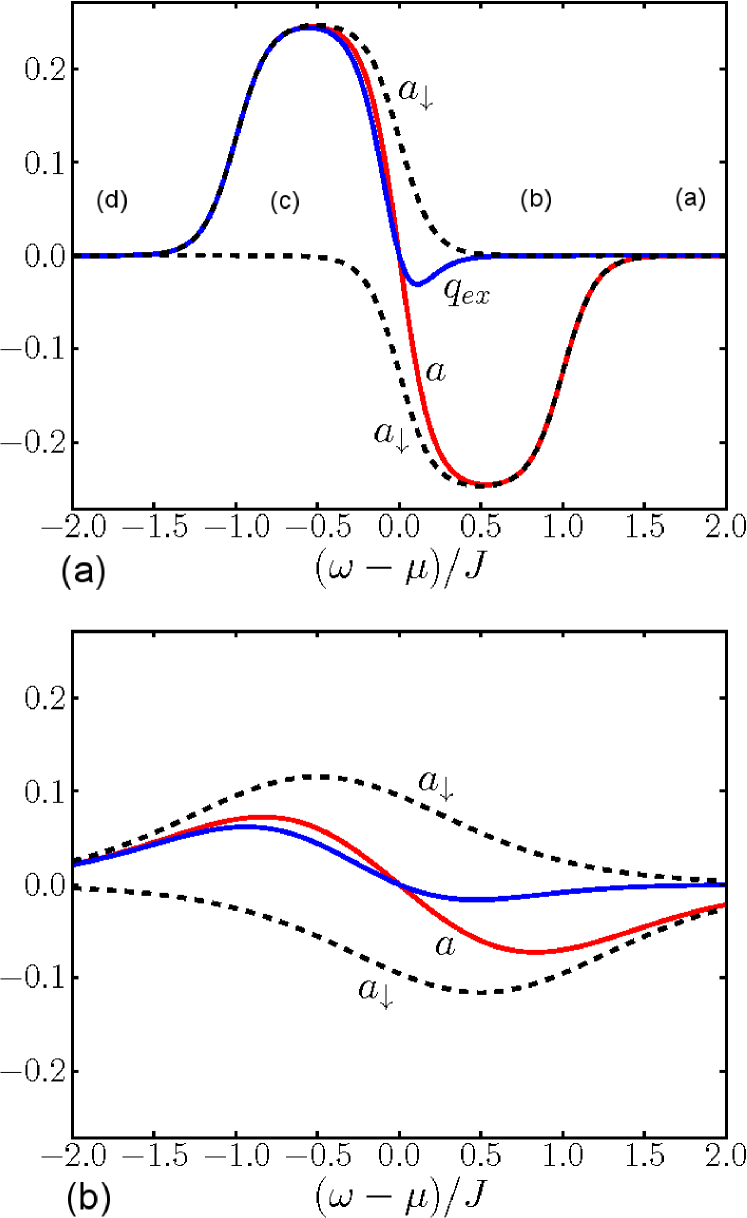
Figure 7: Average local exchange quadrupolarization $q_{\mathrm{ex}}(\omega)$ (blue), spin anisotropy $a(\omega)$ (red) and its two contributions $a_{\uparrow}(\omega)>0$ (broken line) and  $a_{\downarrow}(\omega)<0$ (broken line) as function of $(\omega-\mu)\text{/}J$ for two temperatures $T\text{/}J=0.1$  in (a) and $T\text{/}J=0.5$ in (b). As $T$ approaches $J$ from below, the weight of $a_{\uparrow}(\omega)$ ($a_{\downarrow}(\omega)$) considerably shrinks (rises) and $q_{\mathrm{ex}}(\omega)$ is strongly suppressed. See also Sect. III.2.6.

We first discuss the shape of $a_{\sigma}(\omega)$ for $\sigma=\uparrow,\downarrow$ for low temperature $4T\text{/}J<1$ translating the arguments of the microscopic picture of Fig. 6 into energy space in Fig. 8. As mentioned, the function $a_{\sigma}(\omega)$ characterizes the single-orbital SQM for a spin $\sigma$ occupying a mode at energy $\omega$ and displays four regimes (in the following $\sim$ means ‘”up to thermal smearing $T$”). These are marked (a)-(d) in Fig. 7 (a) and correspond to the regimes in Fig. 8. We discuss them now in detail:

(a) $\omega\gtrsim\mu+J$ $\Rightarrow$ $a_{\uparrow}(\omega)=a_{\downarrow}(\omega)=0$: there are no occupied states at energy $\omega$, so no exchange correction is needed.

(b) $\mu\lesssim\omega\lesssim\mu+J$ $\Rightarrow$ $a_{\downarrow}(\omega)<0,a_{\uparrow}(\omega)=0$: if a spin-$\uparrow$ is in the first copy, the corresponding mode in the second copy has vanishing probability to be occupied with electrons of any spin since both $\varepsilon_{k\uparrow}=\omega\gtrsim\mu$ and $\varepsilon_{k\downarrow}=\omega+J\gtrsim\mu$. Thus, similar to regime (a), no exchange correction for spin-$\uparrow$ electrons is needed and we obtain $a_{\uparrow}(\omega)=0$. In contrast, if a spin-$\downarrow$  is in the first copy, the corresponding mode in the second copy is predominantly occupied with spin-$\uparrow$ because $\varepsilon_{k\downarrow}=\omega\gtrsim\mu$, but $\varepsilon_{k\uparrow}=\omega-J\lesssim\mu$. This contributes negatively to direct SQM, resulting in $a_{\downarrow}(\omega)<0$.

(c) $\mu-J\lesssim\omega\lesssim\mu$ $\Rightarrow$ $a_{\uparrow}(\omega)>0,a_{\downarrow}(\omega)=0$: if in this case a spin-$\uparrow$ is in the first copy, the corresponding mode in the second copy is also mostly occupied with spin-$\uparrow$ since $\varepsilon_{k\uparrow}=\omega\lesssim\mu$, but $\varepsilon_{k\downarrow}=\omega+J\gtrsim\mu$. This gives a positive correction to the direct SQM. In contrast, $a_{\downarrow}(\omega)=0$ as $\varepsilon_{k\downarrow}=\omega$ and $\varepsilon_{k\uparrow}=\omega-J$ refers to a mostly doubly occupied mode in the second copy, which has a vanishing direct SQM contribution (cf. case (d)).

(d) $\omega\lesssim\mu-J$ $\Rightarrow$ $a_{\uparrow}(\omega)=a_{\downarrow}(\omega)=0$: the corresponding orbital deep inside the Fermi sea is doubly occupied: $f(\varepsilon_{k\uparrow})=f(\varepsilon_{k\downarrow})=1$. By  Eq. (64) the direct SQM due to both spin-$\uparrow$ and spin-$\downarrow$-electrons cancel each other.

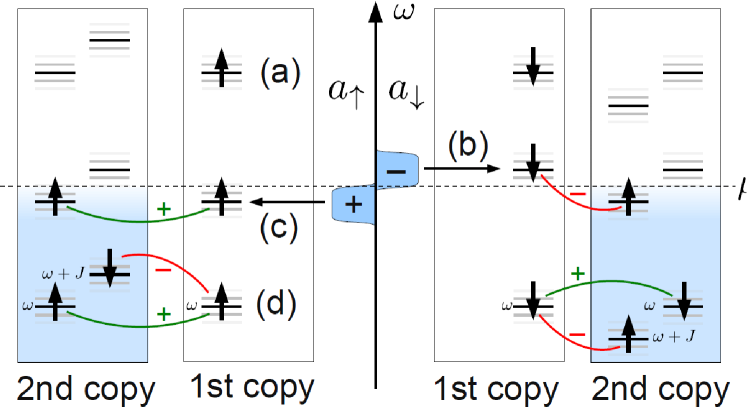
Figure 8: Microscopic picture of the spin-quadrupolarization function $a_{\sigma}(\omega)$, $\sigma=\uparrow,\downarrow$ characterizing the energy resolved spin-anisotropy content of a ferromagnet (cf. Fig. 6), see text.

Altogether, the anisotropy function $a(\omega)=\sum_{\sigma}a_{\sigma}(\omega)$ is exactly antisymmetric with respect to the electrochemical potential (see Fig. 7 and App. A.3)

$$a(\mu+\omega) = -a(\mu-\omega).$$ (71)

As mentioned at the outset, the average exchange quadrupolarization $q_{\mathrm{ex}}(\omega)=f_{+}(\omega)[a_{\uparrow}(\omega)+a_{\downarrow}(\omega)]$ has both positive and negative contributions; however, $q_{\mathrm{ex}}>0$ as the integrated $q_{\mathrm{ex}}(\omega)$ in Eq. (66) is always positive by Eq. (64). At $T=0$ only positive correlations at $\omega<\mu$ count, and we recover the result (38). For $T>0$, thermally excited spins $\downarrow$ negatively correlate with spins $\uparrow$ in the same orbital, thus reducing $q_{\mathrm{ex}}$ (see Fig. 7). Eventually at $T\gg J$ this cancellation reduces $q_{\mathrm{ex}}$ exactly to zero without ever becoming negative. We now see explicitly that the exchange SQM only becomes thermally suppressed for $T\gg J$.

The average exchange quadrupolarization makes explicit that Pauli-forbidden triplet correlations are stored by electrons in an energy window $\sim 2J$ with opposite signs above and below the Fermi energy. Thus, the integrated exchange quadrupolarization is thermally suppressed for $T\gg J$ when the occupation probability  is nearly constant across the energy scale $J$.

III.2.6 Parameter Dependence of Average Exchange SQM

In the flat band approximation (cf. Sect. II.4),  the integral (66) can be carried out yielding (see App. A.4)

$$q_{\mathrm{ex}} = \left.\frac{\bar{\nu}T}{2}\left[\frac{J}{2T}\coth\left(\frac{J}{2T}\right)\right.-1\right],$$ (72)

which is positive since $x\coth(x)>1$, in agreement with the above discussion. In the limit $J\text{/}T\rightarrow 0$, $q_{\mathrm{ex}}$ vanishes as it should (see above) and in the opposite limit of $T\text{/}J\rightarrow 0$, $q_{\mathrm{ex}}$ scales linearly with $N_{s}$, the number of free spins in the ferromagnet (cf. Eq. (27)),

$$\begin{array}[]{lllll}q_{\mathrm{ex}}|_{T=0}&=&\tfrac{1}{4}\bar{\nu}J&=&\tfrac{1}{4}N_{s}\end{array},$$ (74)

in accordance with the $T=0$ result (31). The average one-particle spin-dipole moment $\langle S_{z}\rangle_{T=0}=\tfrac{1}{2}N_{s}$ thus basically serves as a reference scale for two-particle $q_{\mathrm{ex}}$ (when multiplied by $\hbar=1$ in our units). The low $T<J$ behavior is most interesting because in the regime $J<T$ the results do not apply to a Stoner ferromagnet, for which the self-consistent magnetization $J$ would break down (our model Fig. 1 (a) assumes fixed $J$). However, considering our model as a description of mesoscopic islands in an external magnetic field of strength $B=J$ (Fig. 1 (b), this range may also be relevant. With this in mind we show in Fig. 9 the pronounced temperature dependence of the exchange SQM (normalized to the spin polarization) over the entire range for fixed $J$. This should be contrasted with the average spin for which all $T$-dependence completely cancels out due to the constancy of the assumed DOS. As already anticipated in Sec. II.3, a two-particle quantity, the SQM, probes more of the electronic structure of the ferromagnets than the one-particle charge and spin-dipole moment do.

Figure 9: Magnitude of the local exchange SQM, $q_{\mathrm{ex}}$, normalized to $\langle S_{z}\rangle=N_{s}/2$ as a function of temperature $T\text{/}J$ for $\bar{\nu}=N_{o}\text{/}2D$, $D=25J$, $\mu=0$.

In  Fig. 10, we plot  the dependence of the exchange SQM (72) on the Stoner splitting $J$, illustrating that while $\left|\langle\mathbf{S}\rangle\right|$ scales linearly with $J$, $\langle\bm{\mathcal{Q}}\rangle_{\mathrm{ex}}$ initially increases quadratically and then approaches a linear asymptote:

$$q_{\mathrm{ex}} = \tfrac{\bar{\nu}T}{4}\left\{\begin{array}[]{ll}(J\text{/}T)^{2}/6&J\text{/}T\ll 1\\ (J\text{/}T)-2&J\text{/}T\gg 1\end{array}\right..$$ (77)

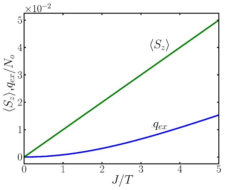
Figure 10: Magnitude of the spin $\langle S_{z}\rangle\approx N_{s}/2=N_{o}J/2D$ (green) (Eq. (26)) and the exchange SQM $q_{\mathrm{ex}}$ (Eq. (72)) (blue) as a function of Stoner splitting $J\text{/}T$ for $\bar{\nu}=N_{o}\text{/}(2D)$, $D=25T$, $\mu=0$.

IV Spin-Multipole Current Operators

We now turn to the third central question posed in the introduction - the proper definition of the SQM current operator.  In the previous section, we answered the important question from where and to where SQM can be transported in terms of nodes in a spin-multipole network, cf. III.2.2. We now investigate the links between the nodes in this network, which correspond to the SQM current operators as noted at the end of Sec. III.2. Their definition and physical interpretation requires some care because (i) like the spin, the total SQM is not conserved in a device comprising Stoner ferromagnets and (ii) unlike the spin, this two-particle quantity does not flow directly between local nodes, but is buffered in non-local nodes.

To tackle point (i), we first revisit the one-particle charge and spin current operator. The spin-dipole current does not have the intuitive definition similar to the charge current (total outgoing current = rate of loss of charge) since the spin is not conserved internally in the ferromagnets. Starting from continuity equations in integral form, the spin currents rather have to be defined as the change in spin induced by the tunneling. In close analogy, we derive SQM current operators obeying a continuity equation and current conservation laws.

Due to point (ii), we have also consider SQM current operators, accounting for the flow of SQM between local and non-local nodes. These turn out to be of central physical importance and reflect that on a microscopic level SQM is carried by pairs of correlated spin dipoles. The flow of spin anisotropy in an electronic system is thus inherently a two-particle process. We will see that, as a result, the layout of the physical device and the network for SQM transport are different: the 2-terminal spin-valve requires a serial 3-node SQM network. For more complex devices even the connectivity is different Hell and Wegewijs (2013).

IV.1 Charge and Spin-Dipole Current

The physical quantities of interest are the rates of change in local quantities in the physical subsystems of the circuit due to transport processes. For one-particle quantities such as charge and spin the physical subsystems are in one-to-one correspondence with the nodes of the charge / spin network, cf. Fig. 5. The time derivative operator $\dot{R}^{r}_{\mu}(t)$ giving the rate of change in the combined charge-spin one-particle operator $R^{r}_{\mu}$ (cf. Eq. (41)), $\tfrac{\mathrm{d}}{\mathrm{d}t}\langle R^{r}_{\mu}(t)\rangle=\langle\dot{R}^{r}_{\mu}(t)\rangle$, is given by

$$\dot{R}^{r}_{\mu}(t) := i[H,R^{r}_{\mu}],$$ (78)

exploiting the von-Neumann equation $\dot{\rho}(t)=-i[H,\rho(t)]$ and the cyclic invariance of the trace $\mathrm{tr}(R^{r}_{\mu}\dot{\rho}(t))=\mathrm{tr}(i[H,R^{r}_{\mu}]\rho(t))$. We next decompose the total system Hamiltonian $H$ into the part describing the decoupled subsystems, $H_{0}$, and the tunneling $H_{T}=\sum_{\langle rs\rangle}H_{T}^{rs}$ with $H_{T}^{rs}$ only accounting for tunneling processes between a pair of nodes $r$ and $s$. This yields a continuity equation in integral form for operators,

$$\dot{R}^{r}_{\mu}(t) = \dot{R}^{r}_{\mu}(t)|_{0}+\sum_{s\neq r}I_{R_{\mu}}^{rs},$$ (79)

which decomposes the total rate of change in the charge (spin) operator in node $r$ into two physically meaningful contributions: The first contribution to Eq. (79) is given by

$$R_{\mu}^{r}|_{0} = i[H_{0},R_{\mu}^{r}]$$ (80)

and accounts for the time-evolution due to internal processes in node $r$. We will depict this contribution in the network picture in  Fig. 11 by an external arrow attached to node $r$. The second part $I_{R_{\mu}}^{r}=\sum_{s\neq r}I_{R_{\mu}}^{rs}=i[H_{T},R_{\mu}^{r}]$ quantifies the rate of change induced by tunneling, i. e., this defines the current of observable $R_{\mu}^{r}$ into node $r$. In the form of Eq. (79), it has already decomposed into its various contributions emanating from all other subsystems $s$:

$$I_{R_{\mu}}^{r} = \sum_{s\neq r}I_{R_{\mu}}^{rs},$$ (81)

Whenever the operator $I_{R_{\mu}}^{rs}\neq 0$, we depict this in the network picture by an arrow inking the two nodes $r$ and $s$. Note that still the average current $\langle I_{R_{\mu}}^{rs}\rangle$ that flows between the nodes may vanish, e. g., for a some special set of parameters. So far, our considerations are quite general and also apply to systems including quantum dots.

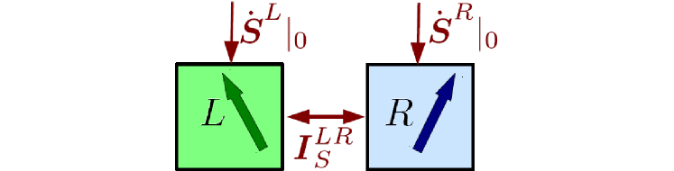
Figure 11: Network picture for the spin with current operators represented by links. The network picture for charge is similar, but without external arrows pointing to the nodes (indicated by $\dot{\mathbf{S}}^{r}|_{0}$). The latter must be introduced due to the internal violation of spin conservation in each spin-node

In our model (Eqs. (7)-(9)), the particle number $R^{r}_{0}=N^{r}$ is conserved internally in each electrode individually and therefore

$$\begin{array}[]{lllll}N^{r}|_{0}&=&[H_{0},N^{r}]&=&0\end{array},$$ (83)

which is the 0-component of Eq. (80) and $\dot{N}=\sum_{\alpha}I_{N}^{\alpha}$.  These make up for the total change in charge. The spin $R^{r}_{i}=S^{r}_{i}$ ($i\neq 0$), however, is not conserved internally in the ferromagnets:

$$\begin{array}[]{lll}\dot{\mathbf{S}}^{\alpha}&=&\dot{\mathbf{S}}^{r}|_{0}+\mathbf{I}^{\alpha}_{\mathbf{S}}\end{array},$$ (84)

where $\mathbf{I}^{\alpha}_{\mathbf{S}}$ is the operator for spin-current into node $\alpha$. Using Eq. (8), one finds

$$\begin{array}[]{lllll}\dot{\mathbf{S}}^{r}|_{0}&=&\sum_{n}J_{n}^{r}\hat{\mathbf{J}}^{r}\times\mathbf{S}^{r}_{n}&\neq&0\end{array}$$ (85)

for $\mathbf{S}^{r}_{n}=\sum_{k\sigma}\mathbf{s}^{r}_{\sigma\sigma^{\prime}}c^{{\dagger}}_{rnk\sigma}c_{rnk\sigma}$ being the contribution from band $n$ to the spin of electrode $r$. This describes a precession of $\mathbf{S}^{r}_{n}$ about the Stoner field of electrode $r$.

To obtain an explicit starting point for the real-time calculation of the average charge and spin current (see App. E), we use Eq. (80) and Eq. (9) and recover the familiar form of the charge and spin current operators,

$$I^{rs}_{R_{\mu}} = \sum_{nn^{\prime}kk^{\prime}\sigma\sigma^{\prime}}(-ir_{\mu}T)^{rs}_{\sigma\sigma^{\prime}}c^{{\dagger}}_{rnk\sigma}c_{sn^{\prime}k^{\prime}\sigma^{\prime}}-\text{h.c.},\,$$ (86)

abbreviating the matrix product in spin-space $(r_{\mu}T)^{rs}_{\sigma\sigma^{\prime}}=\sum_{\tau}(r_{\mu})_{\sigma\tau}T^{rs}_{\tau\sigma^{\prime}}$. The operator (86) describes the net current injected from node $s$ into $r$, accounting for tunneling processes from node $s$ to $r$ (the first contribution in Eq. (86)) and the reverse process (the second). Only the sum of both terms is a Hermitian operator and therefore a physical observable. Since both processes contribute with an opposite sign to the current (86), we obtain the antisymmetry relation $I_{R_{\mu}}^{rs}=-I_{R_{\mu}}^{sr}$. This has an important physical consequence: summing up all charge (spin) currents in the system yields the zero operator:

$$\sum_{r}\sum_{s\neq r}I^{rs}_{R_{\mu}} = 0.$$ (87)

This charge (spin) current conservation law expresses that charge (spin) is conserved by tunneling, that is $[H_{T},R^{\mathrm{tot}}_{\mu}]=0$. Since the total spin is not conserved under the full time evolution (due to the internal evolution $\dot{\mathbf{S}}^{\mathrm{tot}}|_{0}\neq 0$), there is no analogue of Eq. (87) for the total time derivative $\dot{\mathbf{S}}^{r}$. We emphasize furthermore that this conservation law holds on an operator level and not only for expectation values.

IV.2 Spin-quadrupole Current

We now try to proceed analogously for the SQM network in Fig. 5 of Sec. III.2. Generally, we are interested in finding the rate of change in the spin anisotropy stored in local nodes. To this end, we need to consider the change in SQM, $\dot{\bm{\mathcal{Q}}}^{rr^{\prime}}$, in both the local nodes ($r=r^{\prime}$) and the non-local nodes ($r\neq r^{\prime}$). Taking the time derivative of Eq. (56) and using Eq. (79) we obtain:

$$\dot{\bm{\mathcal{Q}}}^{rr^{\prime}} = \dot{\bm{\mathcal{Q}}}^{rr^{\prime}}|_{0}+\sum_{\langle ss^{\prime}\rangle\neq\langle rr^{\prime}\rangle}\bm{\mathcal{I}}_{\bm{\mathcal{Q}}}^{rr^{\prime},ss^{\prime}},$$ (88)

where $\langle ss^{\prime}\rangle$ denotes the sum over pairs of indices $ss^{\prime}$ (i.e., ignoring their order). This is the continuity equation in integral form for the change in SQM in node $\langle rr^{\prime}\rangle$. The first term is the change in SQM due to the internal time evolution

$$\dot{\bm{\mathcal{Q}}}^{rr^{\prime}}|_{0} = \tfrac{g^{rr^{\prime}}}{2}\left[\dot{\mathbf{S}}^{r}|_{0}\odot\mathbf{S}^{r^{\prime}}+\mathbf{S}^{r}\odot\dot{\mathbf{S}}^{r^{\prime}}|_{0}+(r\leftrightarrow r^{\prime})\right],$$ (89)

which involves the non-zero internal time evolution $\dot{\mathbf{S}}^{r}|_{0}$ given by Eq. (85). Like the spin, the SQM is thus not conserved in any of the nodes in our model. The responsible Stoner fields also effectively exert a “torque” on the SQM, thereby rotating the principal axes of this tensor. Similar to the spin, we depict this in the network picture (Fig. 12) by one-sided arrows pointing at this node.

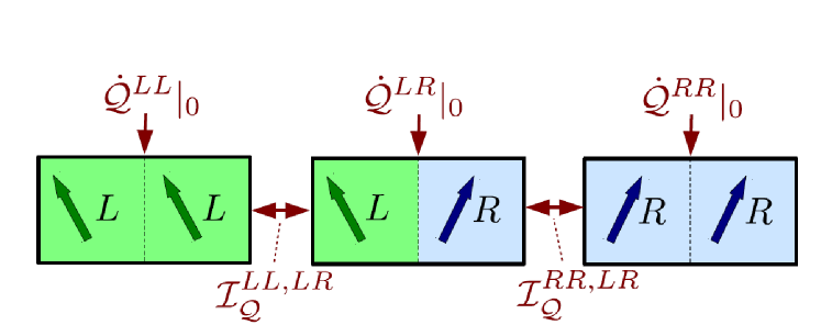
Figure 12: Network picture for SQM including the links representing SQM current operators. Similar to spin, SQM is not conserved internally in the nodes giving rise to external SQM currents.

The SQM current $\bm{\mathcal{I}}_{\bm{\mathcal{Q}}}^{rr^{\prime}}=\sum_{\langle ss^{\prime}\rangle\neq\langle rr^{\prime}\rangle}\bm{\mathcal{I}}_{\bm{\mathcal{Q}}}^{rr^{\prime},ss^{\prime}}$ is given by the Hermitian tensor operator

$$\bm{\mathcal{I}}_{\bm{\mathcal{Q}}}^{rr^{\prime}} = \tfrac{g^{rr^{\prime}}}{2}\left[\mathbf{I}_{\mathbf{S}}^{r}\odot\mathbf{S}^{r^{\prime}}+\mathbf{S}^{r}\odot\mathbf{I}_{\mathbf{S}}^{r^{\prime}}+(r\leftrightarrow r^{\prime})\right].$$ (90)

This is a central result of the paper. Since the spin and the spin current do in general not commute as operators on Fock space, the individual terms in this expression are not Hermitian and therefore not observables. The operator (90) reflects that in general the average SQM current is not simply the product of spin and spin current since $\langle\mathbf{I}_{\mathbf{S}i}^{r}\mathbf{S}^{r^{\prime}}_{j}\rangle\neq\langle\mathbf{I}_{\mathbf{S}i}^{r}\rangle\langle\mathbf{S}_{j}^{r^{\prime}}\rangle$ due to quantum mechanical exchange correlations, interactions, etc. Therefore, SQM is not determined by spin-dipole moment: it requires a separate description in spintronics transport theory. For the bilinear tunnel coupling (9), the contribution to the net current from node $\langle ss^{\prime}\rangle$ into in node $\langle rr^{\prime}\rangle$ is

$$\bm{\mathcal{I}}_{\bm{\mathcal{Q}}}^{rr^{\prime},ss^{\prime}} = \tfrac{g^{rr^{\prime}}}{2}\left[\mathbf{I}_{\mathbf{S}}^{rs}\odot\mathbf{S}^{r^{\prime}}\delta^{r^{\prime}s^{\prime}}+\mathbf{S}^{r}\delta^{rs}\odot\mathbf{I}_{\mathbf{S}}^{r^{\prime}s^{\prime}}\right]$$ (91)

$$+(r\leftrightarrow s^{\prime})].$$

Notably, this SQM current is zero unless one of the indices $s,s^{\prime}$ match the indices $r,r^{\prime}$. This puts an important restriction on the network connectivity: the local SQM nodes are only linked to non-local nodes, and not to other local nodes. Changes of local spin-anisotropy,

$$\dot{\bm{\mathcal{Q}}}^{rr} = \dot{\bm{\mathcal{Q}}}^{rr}|_{0}+\bm{\mathcal{I}}_{\bm{\mathcal{Q}}}^{rr},$$ (92)

which are due to ransport thus only occur through changes in non-local spin correlations:

$$\begin{array}[]{lll}\bm{\mathcal{I}}_{\bm{\mathcal{Q}}}^{rr}&=&\sum_{s\neq r}\left(\mathbf{I}_{\mathbf{S}}^{rs}\odot\mathbf{S}^{r}+\mathbf{S}^{r}\odot\mathbf{I}_{\mathbf{S}}^{rs}\right),\end{array}$$ (94)

where $\mathbf{I}_{\mathbf{S}}^{rs}$ is the spin-current operator from node $s$ into $r$.

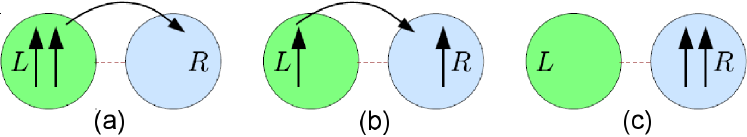
Figure 13: Illustration of the microscopic picture of SQM transport. (a) Consider two electrons in electrode $L$ that contribute to the SQM of the local node $\langle LL\rangle$. (b) By transferring one of these electrons to subsystem $R$, the local spin-spin correlation is lost but a new non-local correlations are established, increasing the SQM of node $\langle LR\rangle$. Thus, emitting spin-polarized electrons non-local correlations are set up in the circuit. (c) When the second electron follows the first, local SQM correlations are created, but now in subsystem $R$ (node $\langle RR\rangle$). Note that this picture is only meant to illustrate the non-locality aspect of SQM, but incorrectly portrays the spins as distinguishable objects.

All the considerations so far in this section were are general. For the simple spin-valve we consider n this paper the general theory above implies that SQM cannot be directly transferred from the local node $\langle LL\rangle$ to the local node $\langle RR\rangle$; it is rather first “buffered” in the intermediate, non-local node $\langle LR\rangle$. This restriction on the SQM network connectivity is related to the real-space picture of  SQM transport sketched in Fig. 13. This picture unveils why SQM transport is possible even in the single electron transport limit (leading order in $H_{T}$), as discussed for spin-values with embedded spin-isotropic quantum dots Sothmann and König (2010); Baumgärtel et al. (2011); Misiorny et al. (2012a). In this case we have on the right hand side of Eq. (92) $\dot{\bm{\mathcal{Q}}}^{rr}|_{0}=0$ where $r$ now labels the quantum dot embedded in this spin-valve. Then SQM currents are responsible for the change in the local QD spin-anisotropy of a subsystem $r$, i. e. $\dot{\bm{\mathcal{Q}}}^{rr}=\bm{\mathcal{I}}_{\bm{\mathcal{Q}}}^{rr}$ where $\bm{\mathcal{I}}_{\bm{\mathcal{Q}}}^{rr}$ of Eq. (94) was already obtained in Ref. Baumgärtel et al. (2011) for a spin-valve with an embedded quantum dot, however, without using the new network picture. The calculations in Baumgärtel et al. (2011) demonstrate that in such more complicated devices the SQM current $\bm{\mathcal{I}}_{\bm{\mathcal{Q}}}^{rr}$, averaged over the non-equilibrium state, depends non-trivially on the average accumulated charge and spin of the dot. The SQM current thus couples to measurable charge and spin currents and should in general be considered for the description of spin and charge dynamics.

Analogous to the charge and spin current the SQM current (91) is antisymmetric with respect to the node indices, i.e., when the two pairs of subsystem-indices $rr^{\prime}$ and $ss^{\prime}$ are interchanged:  $\bm{\mathcal{I}}_{\bm{\mathcal{Q}}}^{rr^{\prime},ss^{\prime}}=-\bm{\mathcal{I}}_{\bm{\mathcal{Q}}}^{ss^{\prime},rr^{\prime}}$. (Note that the order of indices denoting a pair does not matter, i.e., $rr^{\prime}=r^{\prime}r$). As a consequence, the SQM currents sum to the zero tensor operator:

$$\sum_{\langle rr^{\prime}\rangle}\bm{\mathcal{I}}_{\bm{\mathcal{Q}}}^{rr^{\prime}} = \sum_{\langle rr^{\prime}\rangle}\sum_{\langle ss^{\prime}\rangle\neq\langle rr^{\prime}\rangle}\bm{\mathcal{I}}_{\bm{\mathcal{Q}}}^{rr^{\prime},ss^{\prime}}=0.$$ (95)

Similar to spin, this SQM current conservation law expresses the conservation of total circuit SQM (51) in the tunneling. This is a direct consequence of the total spin-dipole conservation by tunneling: $\left[H_{T},\bm{\mathcal{Q}}^{\mathrm{tot}}\right]=\mathbf{S}^{\mathrm{tot}}\odot\left[H_{T},\mathbf{S}^{\mathrm{tot}}\right]+\left[H_{T},\mathbf{S}^{\mathrm{tot}}\right]\odot\mathbf{S}^{\mathrm{tot}}=0$.

Finally, we note that the restriction on the network connectivity found above derives from the particular form of our tunneling Hamiltonian (9), which is bilinear in the field operators. The network thus describes the connectivity on the operator level. The topology of this network is different when $H_{T}$ is, e.g., an effective exchange coupling that is quartic in the fields. Since such a coupling is usually derived from the bilinear tunneling model (9) studied here, we will not dwell on this further.

V Average Spin-Multipole Currents

In this section we complete the discussion of the third main question posed in the introduction: we present explicit results for the average spin-quadrupole current calculated to first order in the tunnel coupling $\Gamma$ of the two ferromagnets and compare it to the average charge and spin current. The calculations of these are compactly presented in in App. D, applying a covariant reformulation of the real-time diagrammatic technique (for a systematic, self-contained technical presentation see App. E). Covariance is used here in the sense that all expressions are form-invariant under a change of the spatial coordinate system and the spin quantization axis. An advantage of this technique is that it can be extended to spin-valves with embedded quantum dots Hell and Wegewijs (2013).

In Sec. V.1 we discuss the results for a general multi-band dispersion relation $\varepsilon^{r}_{nk\sigma}$, applying the insights obtained from the spin-multipole network theory developed in III.2.2 and IV and the microscopic picture explained in III.2.4. We decompose the SQM current into physically meaningful contributions: direct vs. exchange (Pauli exclusion hole aspects) and dissipative vs. coherent (quantum fluctuation aspects). An intimate connection between storage (see III) and transport of charge, spin and SQM is then established by comparing their energy-resolved contributions (see Sec. III.2.5).

In Sec. V.2 we specialize to the flat band approximation (cf. II.4) to obtain tangible analytical and numerical results. Even in this simple limit – where the dissipative spin-current vanishes due to the energy independent DOS – the average SQM current tensor has a non-trivial parameter dependence. This concerns both its magnitude (principal values) and its alignment (principal vectors), which are substantially controllable by magnetic and electric parameters for non-collinear Stoner vectors.

In Sec. V.3 we demonstrate that a pure SQM current, i. e., not accompanied by a spin current, is in principle possible. This spin-anisotropy transfer is entirely carried by Pauli exclusion holes, giving rise to a non-vanishing exchange SQM current. For a temperature bias between ferromagnets with collinear Stoner vectors, we even show that a pure SQM currents even persists in the absence of a charge current. Electrodes with non-trivial spin structure can thus “talk” to each other in ways not described by charge and spin currents

V.1 Charge, spin and SQM current

The average charge, spin and spin-quadrupole current associated with the left electrode read

$$\langle I^{L}_{N}\rangle = I_{N,0}^{L}+I^{L}_{N,F}\left(\widehat{\mathbf{J}}^{L}\cdot\widehat{\mathbf{J}}^{R}\right),$$ (96)

$$\langle\mathbf{I}^{L}_{\mathbf{S}}\rangle = E_{\mathbf{S}}^{L}\widehat{\mathbf{J}}^{L}+A^{L}_{\mathbf{S}}\widehat{\mathbf{J}}^{R}+T^{L}_{\mathbf{S}}\left(\widehat{\mathbf{J}}^{L}\times\widehat{\mathbf{J}}^{R}\right),$$ (97)

$$\langle\bm{\mathcal{I}}^{LL}_{\bm{\mathcal{Q}}}\rangle = 2\left\langle\mathbf{S}^{L}\right\rangle\odot\langle\mathbf{I}^{L}_{\mathbf{S}}\rangle-$$ (98)

$$\widehat{\mathbf{J}}^{L}\odot\left[E_{\mathrm{ex}}^{L}\widehat{\mathbf{J}}^{L}+A^{L}_{\mathrm{ex}}\widehat{\mathbf{J}}^{R}+T^{L}_{\mathrm{ex}}\text{ }\widehat{\mathbf{J}}^{L}\times\widehat{\mathbf{J}}^{R}\right]$$

These were calculated in App. D to the first order in the energy-resolved tunneling rate

$$\Gamma(\omega) = 2\pi t^{2}\bar{\nu}^{L}(\omega)\bar{\nu}^{R}(\omega),$$ (99)

where $\bar{\nu}^{r}(\omega)$ is given by Eq. (14). Here $\odot$ denotes the symmetric, traceless tensor product (52). The charge current coefficients are (we will not write the $\omega$ dependence unless confusion may arise)

$$I_{N,0} = \int\mathrm{d}\omega 2\Gamma\Delta,$$ (100)

$$I^{L}_{N,F} = \int\mathrm{d}\omega 2\Gamma\Delta n^{L}n^{R},$$ (101)

where the spin-polarization function $n^{r}(\omega)$ is given by Eq. (15). The well-known bias function,

$$\Delta(\omega) = f^{R}_{+}(\omega)-f^{L}_{+}(\omega),$$ (102)

is only non-zero in the bias window, $\mu^{L}\gtrsim\omega\gtrsim\mu^{R}$, up to thermal smearing. The occurrence of the factor $\Delta(\omega)$ signals that a term arises from dissipative processes in which the energy of initial and final state have to be the same. The spin current coefficients are

$$E^{L}_{\mathbf{S}} = \int\mathrm{d}\omega\Gamma\Delta n^{L},$$ (103)

$$A^{L}_{\mathbf{S}} = \int\mathrm{d}\omega\Gamma\Delta n^{R},$$ (104)

$$T^{L}_{\mathbf{S}} = \int\mathrm{d}\omega\Gamma\left(\beta^{L}\frac{n^{R}}{\bar{\nu}^{L}}+\beta^{R}\frac{n^{L}}{\nu^{R}}\right),$$ (105)

the function $\beta^{r}(\omega)$ incorporates the effect of the spin-polarization of the DOS, $n^{r}(\omega)$, through the principal value integral,

$$\beta^{r}(\omega) = \mathrm{Re}\int\frac{d\omega^{\prime}}{\pi}\frac{\bar{\nu}^{r}(\omega^{\prime})n^{r}(\omega^{\prime})f^{r}_{+}(\omega^{\prime})}{\omega-\omega^{\prime}+i0},$$ (106)

integrating over all virtual state energies $\omega^{\prime}$. Here and below such functions, not limited by energy conservation as they involve virtual intermediate states, appear in contributions from coherent processes. Finally, the exchange SQM emission, absorption and torque coefficients

$$E^{L}_{\mathrm{ex}} = 2\int\mathrm{d}\omega\Gamma\Delta a^{L},$$ (107)

$$A^{L}_{\mathrm{ex}} = 2\int\mathrm{d}\omega\Gamma\Delta n^{R}\tilde{a}^{L},$$ (108)

$$T^{L}_{\mathrm{ex}} = 2\int\mathrm{d}\omega\Gamma(\alpha^{R}f^{L}_{+}-\beta^{R})\frac{a^{L}}{\bar{\nu}^{R}},$$ (109)

depend on the local spin-anisotropy function $a^{L}$, cf. (68), and an additional even spin-anisotropy function,

$$\tilde{a}^{L}(\omega) = \int\mathrm{d}\omega^{\prime}f^{r}_{+}(\omega^{\prime})\sum_{\sigma,\sigma^{\prime}}\frac{\sigma^{\prime}}{4}\frac{\nu^{r}_{\sigma\sigma^{\prime}}(\omega,\omega^{\prime})}{\bar{\nu}^{r}(\omega)}$$ (110)

$$= \sum_{\sigma}\sigma a_{\sigma}^{r}(\omega),$$ (111)

where $\nu^{r}_{\sigma\sigma^{\prime}}(\omega,\omega^{\prime})$ is the 2DOS (16).  Finally, the torque coefficient $T^{L}_{\bm{\mathcal{Q}}}$ involves an additional function similar to Eq. (106) but without the distribution function $f_{+}^{R}(\omega)$ under the principal value integral:

$$\alpha^{R}(\omega) = \mathrm{Re}\int\frac{d\omega^{\prime}}{\pi}\frac{n^{R}(\omega^{\prime})\bar{\nu}^{R}(\omega^{\prime})}{\omega-\omega^{\prime}+i0}.$$ (112)

The reader should note that the coefficients of Eqs. (107)-(109) are defined such that a minus sign appears in Eq. (98), which we introduced in agreement with the sign convention for exchange SQM in Eq. (63), that is, $\langle\bm{\mathcal{Q}}^{LL}\rangle=-q_{\mathrm{ex}}^{L}\widehat{\mathbf{J}}^{L}\odot\widehat{\mathbf{J}}^{L}$. Moreover, one obtains the expressions for $\langle\bm{\mathcal{I}}^{RR}_{\bm{\mathcal{Q}}}\rangle$ by formally substituting $L\leftrightarrow R$ in Eq. (98), and $\langle\bm{\mathcal{I}}^{LR}_{\bm{\mathcal{Q}}}\rangle=-\langle\bm{\mathcal{I}}^{LL}_{\bm{\mathcal{Q}}}\rangle-\langle\bm{\mathcal{I}}^{RR}_{\bm{\mathcal{Q}}}\rangle$ follows from the SQM current conservation law (95) (see also below). One checks that the results are invariant under scalar gauge transformations (global energy shifts). Finally, we note that since positive currents are defined as entering a node, positive (negative) absorption coefficients correspond to injection (ejection) of particles and vice versa for emission coefficients.

The SQM current Eq. (98) is the central result of this paper. It depends explicitly (but not exclusively) on the spin current (97). Therefore, its physical interpretation is aided by first giving a pertinent review of the different contributions to the charge and spin-currents (96) and (97), respectively.

V.1.1 Charge Current

Eq. (96) is a well-known and experimentally tested result for the charge current, which accounts for single electron tunneling processes between the left and right electrode. It has only dissipative contributions (i.e., involving $\Delta(\omega)$): the first part $I_{N,0}$ in  Eq. (96) only depends in the average DOS $\bar{\nu}^{r}$ whereas the second, spin-dependent correction that depends on the DOS spin-polarizations $n^{r}$ through $I^{L}_{N,F}$ and on the angle between the Stoner vectors through $\widehat{\mathbf{J}}^{L}\cdot\widehat{\mathbf{J}}^{R}=\cos\theta$. The reduction going from $\theta=0\rightarrow\pi$ is the celebrated spin-valve or tunnel magneto resistance (TMR) effect.

V.1.2 Spin Current

The spin current (97) was obtained by Braun et. al and we review here its two type of contributions.

Dissipative spin emission $\sim\hat{\mathbf{J}}^{L}$ and absorption $\sim\hat{\mathbf{J}}^{R}$

The dissipative spin-dipole current (first two terms in Eq. (97), containing $\Delta(\omega)$) is analogous to the particle current:  an electron emitted from the left node transports a spin-dipole moment $\hat{\mathbf{J}}^{L}/2$ and the electrons absorbed from the right node transports $\hat{\mathbf{J}}^{R}/2$. The expression for particle current Eq. (100) simply has to be supplemented by a factor $n^{r}(\omega)\hat{\mathbf{J}}^{r}/2$ to obtain the terms for spin emission (103) and absorption (104).

Coherent spin torque $\sim\hat{\mathbf{J}}^{L}\times\hat{\mathbf{J}}^{R}$

The coherent spin current (last term in Eq. (97)) has no such analogy to the particle current and corresponds to a spin-torque. This corresponds to spin flips induced by virtual fluctuations between the left and the right electrode restricted by energy conservation only in the final state, but not in the intermediate state. This is reflected by its dependence on the principal value integral $\beta^{r}(\omega)$ (cf. discussion of Eq. (106)): an electron with spin $\sigma$ occupying a level at energy $\omega$ in the left electrode can fluctuate to all empty levels with energy $\omega^{\prime}$ in the right electrode with an amplitude $\propto 1/(\omega-\omega^{\prime})$. While in the right electrode, the electron spin $\propto\hat{\mathbf{J}}^{L}$ is not collinear to the Stoner field $\propto\hat{\mathbf{J}}^{R}$ in the right electrode and precesses about it, explaining the factor $\widehat{\mathbf{J}}^{L}\times\widehat{\mathbf{J}}^{R}$ in the coherent spin current (105). Note that a net spin-torque on the magnetization of the left electrode only occurs if the 1DOS of both electrodes are spin-polarized.

Finally, we note that at zero bias, the dissipative spin-current vanishes, $E_{\mathbf{S}}^{L}=A^{L}_{\mathbf{S}}=0$, but the coherent spin-current (torque contribution) remains, $T^{L}_{\mathbf{S}}\neq 0$: non-collinear ferromagnets keep interacting by virtual fluctuations, thereby exerting a torque on each other.

V.1.3 SQM Current

SQM current conservation

The most immediate property of the SQM current expression (98) is its formal lack of symmetry with respect to interchanging the electrodes $L\leftrightarrow R$. This differs notably from charge and spin current, for which the original expression is reproduced with a minus sign when interchanging $L\leftrightarrow R$. This distinction is related to the striking characteristics of the SQM network picture compared to the charge and spin network (see Sec. V.1.3): the currents of the latter, $\langle I^{L}_{R_{\mu}}\rangle$, describe the net flow into the $L$-node coming from from the $R$-node (see Fig. 11). Interchanging $L$ and $R$ yields then the opposite current from $R$ to the $L$-node, reflecting the current conservation law (87): $\langle I^{L}_{R_{\mu}}\rangle+\langle I^{R}_{R_{\mu}}\rangle=0$. In contrast, $\langle\bm{\mathcal{I}}^{LL}_{\bm{\mathcal{Q}}}\rangle$ describes the net flow of SQM from the local $\langle LL\rangle$-node to the nonlocal $\langle LR\rangle$-node (see Fig. 12). If we interchange $L\leftrightarrow R$ in Eq. (98), we obtain the current $\langle\bm{\mathcal{I}}^{RR}_{\bm{\mathcal{Q}}}\rangle$ emanating from the $\langle RR\rangle$-node. Importantly, $\langle\bm{\mathcal{I}}^{LL}_{\bm{\mathcal{Q}}}\rangle+\langle\bm{\mathcal{I}}^{RR}_{\bm{\mathcal{Q}}}\rangle=-\langle\bm{\mathcal{I}}^{LR}_{\bm{\mathcal{Q}}}\rangle\neq 0$ in accordance with the SQM current conservation law (95). This again emphasizes the relevance of the nonlocal node $\langle LR\rangle$, which “buffers” the SQM currents from both local nodes.

Direct and Exchange SQM Current

The SQM current allows for two physically meaningful, different decompositions. The first decomposition is given by Eq. (98), which breaks up the SQM current into different two-particle contributions, the first, direct term Eq. (98) and the second, exchange term. This has no analogue in the one-particle charge and spin current.

The direct current $\langle\bm{\mathcal{I}}^{LL}_{\bm{\mathcal{Q}}}\rangle_{\mathrm{dir}}$ quantifies the tunneling-induced change in the direct part of the average SQM (59), $\langle\bm{\mathcal{Q}}^{LL}\rangle_{\mathrm{dir}}:=\langle\mathbf{S}^{L}\rangle\odot\langle\mathbf{S}^{L}\rangle$, which ignores the Pauli exclusion hole (cf. Sec. III). Indeed, using Eq. (94), we reproduce the first term in Eq. (98):

$$\langle\bm{\mathcal{I}}^{LL}_{\bm{\mathcal{Q}}}\rangle_{\mathrm{dir}} := \langle\dot{\bm{\mathcal{Q}}}^{LL}-\dot{\bm{\mathcal{Q}}}^{LL}|_{0}\rangle_{\mathrm{dir}}$$ (113)

$$= 2\langle\mathbf{S}^{L}\rangle\odot\langle\mathbf{I}_{\mathbf{S}}^{L}\rangle.$$ (114)

Similar to the average SQM, the direct average SQM current is completely determined by a product of average spin-dipole properties, here the spin $\langle\mathbf{S}^{L}\rangle$ and the spin-current $\langle\mathbf{I}_{\mathbf{S}}^{L}\rangle$, given by Eq. (48) and (97), respectively. This equation substantiates the classical picture of transport SQM or spin-anisotropy sketched in Fig. 13: when single electrons move, the triplet correlations between pairs of electron spins first delocalize and then relocalize, resulting in a change of the local SQM, the part described by $\langle\bm{\mathcal{Q}}^{LL}\rangle_{\mathrm{dir}}$.

The exchange SQM current $\langle\bm{\mathcal{I}}^{LL}_{\bm{\mathcal{Q}}}\rangle_{\mathrm{ex}}$, the second term in Eq. (98),  accounts for the tunnel-induced change in $\langle\bm{\mathcal{Q}}^{LL}\rangle_{\mathrm{ex}}$, i.e., a negative quantum anisotropy due to the Pauli-exclusion holes in the triplet spin correlations. It cannot be expressed in the average spin-current. The above classical picture of SQM transport thus needs correction: by reducing SQM transport to “spin times spin-current” one over-estimates the anisotropy flow, by counting Pauli-forbidden, local triplet correlations (those coming from the same orbital) and accounting for their transformation into non-local correlations when one of the two electrons tunnels out. The SQM exchange current compensates for this: it is an effective back-flow of non-local anisotropy into to the local nodes of the SQM network (Fig. 12). We now reach a central conclusion of the paper: whenever the average spin-current is made to vanish $\langle\mathbf{I}_{\mathbf{S}}^{L}\rangle=0$, a non-zero SQM exchange current is generally present since $\langle\mathbf{S}^{L}\odot\mathbf{I}_{\mathbf{S}}^{L}\rangle\neq\langle\mathbf{S}^{L}\rangle\odot\langle\mathbf{I}_{\mathbf{S}}^{L}\rangle$ due to the Pauli exclusion holes. In Sec. V.3 we explicitly verify that the cancellations of the single-particle contributions that cause the spin-current to cancel have no counterpart for the two-particle exchange SQM current. This indicates the possibility of pure SQM transport, that is, without spin current.

The most prominent distinction between the direct and exchange SQM currents is that they differ by a relative factor $|\langle\mathbf{S}^{L}\rangle|$. To see this explicitly, we express the SQM current (98) as a symmetric, traceless tensor product of the unit vector $\hat{\mathbf{J}}^{L}$ with a linear combination of $\hat{\mathbf{J}}^{L}$, $\hat{\mathbf{J}}^{R}$ and $\hat{\mathbf{J}}^{L}\times\hat{\mathbf{J}}^{R}$ by inserting the explicit spin current (97):

$$\langle\bm{\mathcal{I}}^{LL}_{\bm{\mathcal{Q}}}\rangle = \widehat{\mathbf{J}}^{L}\odot\left[E^{L}_{\bm{\mathcal{Q}}}\widehat{\mathbf{J}}^{L}+A^{L}_{\bm{\mathcal{Q}}}\widehat{\mathbf{J}}^{R}\right]$$ (115)

$$+T^{L}_{\bm{\mathcal{Q}}}\widehat{\mathbf{J}}^{L}\odot(\widehat{\mathbf{J}}^{L}\times\widehat{\mathbf{J}}^{R}),$$

Each of the coefficients has a direct and exchange contribution, respectively:

$$E^{L}_{\bm{\mathcal{Q}}} = 2E^{L}_{\mathbf{S}}\left(\langle\mathbf{S}^{L}\rangle\cdot\hat{\mathbf{J}}^{L}\right)-E_{\mathrm{ex}}^{L},$$ (116)

$$A^{L}_{\bm{\mathcal{Q}}} = 2A^{L}_{\mathbf{S}}\left(\langle\mathbf{S}^{L}\rangle\cdot\hat{\mathbf{J}}^{L}\right)-A_{\mathrm{ex}}^{L},$$ (117)

$$T^{L}_{\bm{\mathcal{Q}}} = 2T^{L}_{\mathbf{S}}\left(\langle\mathbf{S}^{L}\rangle\cdot\hat{\mathbf{J}}^{L}\right)-T_{\mathrm{ex}}^{L}.$$ (118)

Since all coefficients Eq. (103)-(105) and Eq. (107)-(109) appearing on the right hand sides are in general of the same order, the ratio of the direct SQM current to the exchange SQM scales linearly with the average spin $|\langle\mathbf{S}^{L}\rangle|\sim N_{s}=(J/D)N_{o}$ as expected from our analysis below Eq. (62) in Sec. III.2.2. Consequently, for a macroscopic ferromagnet, the SQM current is dominated by its direct part (114) and is thus induced by the spin-current.Furthermore, since the SQM current accounts for the change in the correlations between the spin of a transported electron with all other spins in the system, only the SQM current per electron is expected to be a meaningful quantity in the thermodynamic limit. As soon as one of the subsystems is of meso- or nanoscopic dimensions the relative factor $|\langle\mathbf{S}^{L}\rangle|$ matters (cf. Sec. III.1.2) and the exchange SQM current should be reckoned with. For a nanoscopic system, the full SQM current was already studied in Baumgärtel et al. (2011), while also including the relevant charging and non-equilibrium effects, which were neglected here. With this in mind, we will in the following always first discuss the direct part, dominating the SQM current for macroscopic ferromagnets (Fig. 1 (a)), and then separately consider the exchange correction, relevant for mesoscopic ferromagnets, (Fig. 1 (b)).

Dissipative and Coherent SQM Current

The second, alternative decomposition of the SQM current is that into a dissipative and coherent part, the first and second term of Eq. (115), respectively, similar to the spin-dipole current. For non-collinear $\hat{\mathbf{J}}^{L}$ and $\hat{\mathbf{J}}^{R}$ these terms are linearly independent tensors and their coefficients have very different parameter dependencies. The tensorial structure of the total SQM current is determined by their non-trivial interplay. Its discussion requires explicit results and is therefore postponed to Sec. V.2.3 where we use the flat band approximation.

The decomposition of the direct SQM current follows by Eq. (114) directly from the decomposition of the spin-current (97) into a dissipative emission, dissipative absorption and coherent torque part. Since the exchange SQM current is a correction to the direct current accounting for  Pauli-forbidden triplet correlations, cf. explanation below  Eq. (114), it must have the same decomposition into emission, absorption and torque part with coefficients given by Eqs. (116)-(118), respectively.

Dissipative SQM emission $\sim\widehat{\mathbf{J}}^{L}\odot\widehat{\mathbf{J}}^{L}$ and absorption $\sim\widehat{\mathbf{J}}^{L}\odot\widehat{\mathbf{J}}^{R}$.

The SQM emission can be microscopically understood as the delocalization of triplet spin correlations from node $\langle LL\rangle$ to node $\langle LR\rangle$ (see Fig. 5). The SQM absorption describes the converse relocalization of such correlations from node $\langle LR\rangle$ to node $\langle LL\rangle$. This is reflected by the tensorial structure of these contributions to the average SQM currents: they coincide with the average SQM stored in the node, from where they are emitted ($\widehat{\mathbf{J}}^{L}\odot\widehat{\mathbf{J}}^{L}\sim\langle\bm{\mathcal{Q}}^{LL}\rangle$) or absorbed ($\widehat{\mathbf{J}}^{L}\odot\widehat{\mathbf{J}}^{R}\sim\langle\bm{\mathcal{Q}}^{LR}\rangle$). Importantly, there is no SQM absorption in $\langle\bm{\mathcal{I}}^{LL}_{\bm{\mathcal{Q}}}\rangle$ that originates from the $\langle RR\rangle$-node ( $\widehat{\mathbf{J}}^{R}\odot\widehat{\mathbf{J}}^{R}\sim\langle\bm{\mathcal{Q}}^{RR}\rangle$) as expected from the connectivity in the SQM network picture of Sec. IV.2.

The relation between the storage and transport is also reflected by the integrands of the exchange SQM current in Eqs. (107)-(108): these resemble the average local spin-quadrupolarization $q^{L}_{\mathrm{ex}}(\omega)=f^{L}_{+}(\omega)a^{L}(\omega)$ in the expression (66) for $\langle\bm{\mathcal{Q}}^{LL}\rangle_{\mathrm{ex}}$. These can formally be obtained by a replacement $f_{+}^{L}(\omega)\rightarrow\Delta(\omega)$, i.e., similar to the relation between charge current and the dissipative spin current in Sec. V.1.2. However, the symmetry of the function $a^{L}(\omega)$ with respect to $\omega$ is is very different from that of $n^{L}(\omega)$ appearing the spin current emission (Eq. (103)-(104)). This fact underlies a key result of the paper in Sec. V.3.

The microscopic picture of exchange SQM storage can be extended to capture a precise, physical understanding of the exchange SQM current as follows: as explained in Sect. III.2.4, the Pauli exclusion holes can be “counted” as single-mode cross correlations between two identical copies of the same ferromagnet (cf. Fig. 8). For the exchange SQM current, we have to imagine that the electron in the first copy undergoes a tunneling process (representing to the spin current in Eq. (94)), and the second copy is left unchanged (representing the spin in Eq. (94)). For the dissipative exchange SQM emission, this becomes directly clear from the expression (107): the Fermi function in $\Delta(\omega)$ refers to the electron tunneling at energy $\omega$ in the first copy and the local anisotropy function $a^{L}$ contains the single-mode correlation of that electron with the average (unchanged) second copy. This term therefore describes the flow of Pauli exclusion holes arising from the spin emission $\sim\hat{\mathbf{J}}^{L}$. The exchange coefficient (108) corresponding to the spin absorption $\sim\hat{\mathbf{J}}^{R}$, the the first factor $\Delta n^{R}$ relates to the absorbed spin from the right electrode and the second factor $\tilde{a}^{L}$ represents the correlations of that absorbed spin with the local spins in the left electrode. Notably, the spin-dependent contributions $a^{L}_{\sigma}$ to $a^{L}=\sum_{\sigma}a_{\sigma}^{L}$ are added in $\tilde{a}^{L}=\sum_{\sigma}\sigma a^{L}_{\sigma}>0$ such that they always count as positive. Here the sign of how to count the Pauli-forbidden anisotropy is related to the sign of $n^{R}$: if $n^{R}>0$, mostly spin-$\uparrow$ is absorbed and the missing anisotropy generated by this is positive, while for $n^{R}<0$ mostly spin-$\downarrow$ is absorbed and the missing anisotropy is negative as explained in Sect. III.2.4

Coherent SQM torque $\sim\widehat{\mathbf{J}}^{L}\odot(\hat{\mathbf{J}}^{L}\times\widehat{\mathbf{J}}^{R})$

The coherent contribution to the SQM current basically originates from the spin torque. This follows by considering the direct contribution that derives from the spin current, cf. Eq. (114). It accounts for the change of the correlation between of the spin of an electron fixed in the left electrode with the spin of an electron that virtually fluctuates into the right electrode (spin-flip scattering). Since during this fluctuation the latter spin precesses about the Stoner field and a net conversion of local into non-local correlations results, i.e., there is an associated SQM current. The exchange SQM torque coefficient $T_{\mathrm{ex}}^{L}$ excludes the single-mode correlations: in the microscopic picture only the electron in the first copy undergoes a virtual fluctuation (indicated by $\beta^{R}$ and $\alpha^{R}$ in Eq. (109)) , while the second copy is left unchanged (indicated by $a^{LL}$ in Eq. (109)). This is the effect of the spin torque on the local Pauli-exclusion holes.

V.2 Parameter Dependence

Having discussed the general structure and physical meaning of the main results (96)-(98), we now simplify them as far as possible by making the flat band approximation. Although this is a crude approximation, it reveals a general key feature of the exchange SQM, namely its sensitivity to the spin alignment, a non-negative quantity that accumulates when summing over energies / $k$-modes. This prohibits cancellations in the exchange SQM current as they occur due to  signed contributions in the charge and spin-dipole current. (cf. Sec. III.2.4). As noted in Sec. II.4 the 2DOS appearing in the exchange expressions requires modelling of the electrodes that goes beyond the 1DOS. However, in the flat-band approximation we only need Eq. (192). We furthermore apply the bias voltage symmetrically to the ferromagnets, $\mu^{L}=+V/2$ and $\mu^{R}=-V/2$ while considering arbitrary non-collinear Stoner vectors $\hat{\mathbf{J}}^{L}$ and $\hat{\mathbf{J}}^{R}$. We assume all further parameters to be symmetric: $J^{r}=J$, $T^{r}=T$, $D^{r}=D$ and $\nu^{r}_{\sigma}=\nu_{\sigma}$ for $\sigma=\uparrow,\downarrow$ (except for a temperature gradient discussed in Sec. V.3). In this approximation the densities of states are fixed by the bandwidths, $\nu_{\sigma}=1/2D$, and the tunneling rate is set by the spin-conserving tunnel amplitude $t$: $\Gamma=2\pi(t/2D)^{2}$, cf. Eq. (11). Together with the leading order approximation in $\Gamma$ this limits the applicability of the results to the regime $\Gamma\ll T,J,\ll W$ (cf. Eq. (19)). The central equations (96)-(98) now simplify to

$$\langle I^{L}_{N}\rangle = I_{N,0}^{L},$$ (119)

$$\langle\mathbf{I}^{L}_{\mathbf{S}}\rangle = T^{L}_{\mathbf{S}}\left(\widehat{\mathbf{J}}^{L}\times\widehat{\mathbf{J}}^{R}\right),$$ (120)

$$\langle\bm{\mathcal{I}}^{LL}_{\bm{\mathcal{Q}}}\rangle = 2\left(\langle\mathbf{S}^{L}\rangle\cdot\widehat{\mathbf{J}}^{L}\right)\widehat{\mathbf{J}}^{L}\odot\langle\mathbf{I}^{L}_{\mathbf{S}}\rangle-\widehat{\mathbf{J}}^{L}\odot\left[E_{\bm{\mathcal{Q}}}^{L}\widehat{\mathbf{J}}^{L}+T^{L}_{\bm{\mathcal{Q}}}\left(\widehat{\mathbf{J}}^{L}\times\widehat{\mathbf{J}}^{R}\right)\right]$$ (121)

$$= -E_{\mathrm{ex}}^{L}\widehat{\mathbf{J}}^{L}\odot\widehat{\mathbf{J}}^{L}+\left(2\left(\langle\mathbf{S}^{L}\rangle\cdot\widehat{\mathbf{J}}^{L}\right)T^{L}_{\mathbf{S}}-T^{L}_{\mathrm{ex}}\right)\widehat{\mathbf{J}}^{L}\odot\left(\widehat{\mathbf{J}}^{L}\times\widehat{\mathbf{J}}^{R}\right).$$ (122)

In this approximation the DOS (13) is not spin-polarized in the bias window: $n^{r}(\omega)=0$ for $\mu^{L}\lesssim\omega\lesssim\mu^{R}$. Therefore the charge current  Eq. (119) reduces to its non-magnetic part, i.e., there is no spin-valve effect. By the same token, the dissipative part of the spin current (120) vanishes due to the cancellation of particle and hole contributions. Thus only the coherent spin torque part remains, whose coefficient we now estimate as follows: inserting Eq. (106) into Eq. (105), we obtain

$$T^{L}_{\mathbf{S}} = 2t^{2}\mathrm{Re}\int\mathrm{d}\omega\int\mathrm{d}\omega^{\prime}\prod_{r}(\bar{\nu}^{r}(\omega)n^{r}(\omega))$$ (123)

$$\times\frac{f_{+}^{R}(\omega^{\prime})-f_{+}^{L}(\omega)}{\omega-\omega^{\prime}+i0}.$$

For our DOS approximation, we have $\bar{\nu}^{L}(\omega)n^{L}(\omega)\bar{\nu}^{R}(\omega^{\prime})n^{R}(\omega^{\prime})=\mathrm{sgn}(\omega\omega^{\prime})/(4D)^{2}$ if $|\omega|-D\leqslant J/2$ and $|\omega^{\prime}|-D\leqslant J/2$ and zero otherwise. At these energies the Fermi functions are 0 or 1 and if their difference in Eq. (123) is nonzero, we can approximate $1/|\omega-\omega^{\prime}|\approx 1/(2D)$, yielding

$$T^{L}_{\mathbf{S}} \approx -\frac{\Gamma}{4\pi}\frac{J^{2}}{D}.$$ (124)

where $\Gamma=2\pi|t|^{2}/(2D)^{2}$. The resulting spin current is equivalent to a spin-torque exerted by an magnetic field $\mathbf{B}^{R}\approx\bar{\nu}^{R}J|t|^{2}/D\widehat{\mathbf{J}}^{R}$on the spin on $\mathbf{S}^{L}$ (insert Eq. (26) for $\left|\mathbf{S}^{L}\right|$ into Eq. (120)). Finally, in the SQM current (121)-(122) the absorption coefficient $A_{\bm{\mathcal{Q}}}^{L}$  – and with it, the non-local anisotropy function $a^{LR}$ – drops out in this approximation because of the vanishing of the spin-polarization, $n^{r}(\omega)=0$ in the bias window.

V.2.1 Dissipative SQM Flow Direction

We first discuss the direction of the dissipative spin-anisotropy emission, $\langle\bm{\mathcal{I}}^{LL}_{\bm{\mathcal{Q}}}\rangle=-2E_{\bm{\mathcal{Q}}}^{L}\widehat{\mathbf{J}}^{L}\odot\widehat{\mathbf{J}}^{L}$, which entirely arises from the exchange term in Eq. (121) (the direct part vanishes in absence of dissipative spin current). Remarkably, the emission always results in a loss of local exchange spin-anisotropy $\langle\bm{\mathcal{Q}}^{LL}\rangle_{\mathrm{ex}}=-q^{LL}_{\mathrm{ex}}\hat{\mathbf{J}}^{L}\odot\hat{\mathbf{J}}^{L}$ irrespective of the voltage bias direction, because $E_{\bm{\mathcal{Q}}}^{L}$ is always negative (unless zero). By interchanging the left and right electrode index in all expressions, we  observe that the spin-anisotropy of the $\langle RR\rangle$-node decreases as well. We conclude from the SQM current conservation law that non-local spin-triplet correlations are built up irrespective of the bias direction. This is in accordance with the physical intuition of SQM transport that we have developed using our network picture the tunneling of electrons across the junction delocalizes spin-triplet correlations. However, such a pure delocalization is special to a voltage-biased tunnel junction. When we discuss the situation of thermal bias later, we will see that an effective transfer of spin-anisotropy between the local nodes is still possible.

These results can also be clearly understood in terms of the microscopic picture of SQM storage introduced in Sect. III.2.5. To see this, we first note that the exchange SQM emission (107) is obtained from the average (see Eqs. (66) -(67)) by replacing the Fermi function $f^{L}_{+}$ by the bias function $\Delta$. If $\mu^{L}>\mu^{R}$, electrons leave the left electrode, which is indicated by $\Delta(\omega)>0$ at energies $\mu^{R}\lesssim\omega\lesssim\mu^{L}$. This destroys the positive local exchange SQM content at this energy (given by $a^{L}(\omega)>0$, see also Fig. 7). Conversely, for the opposite bias $\mu^{L}<\mu^{R}$, we find $\Delta(\omega)<0$ for $\mu^{L}\lesssim\omega\lesssim\mu^{R}$ since the tunneling electrons enter the left electrode. Electrons at these frequencies provide negative exchange SQM (as $a^{L}(\omega)<0$). In both cases this results in a negative change in $q^{L}_{\mathrm{ex}}$.

V.2.2 Scalar Parameter Dependence

We next discuss the dependence of the direct and exchange SQM current on the scalar parameters $J$, $V=\mu^{L}-\mu^{R}$ and $T$. For the direct SQM current,

$$\langle\bm{\mathcal{I}}^{LL}_{\bm{\mathcal{Q}}}\rangle_{\mathrm{dir}} = 2\left(\langle\mathbf{S}^{L}\rangle\cdot\widehat{\mathbf{J}}^{L}\right)T^{L}_{\mathbf{S}}\widehat{\mathbf{J}}^{L}\odot\left(\widehat{\mathbf{J}}^{L}\times\widehat{\mathbf{J}}^{R}\right),$$ (125)

this is simple because $T^{L}_{\mathbf{S}}$ is nearly independent of $V$ and $T$ and increases as $J^{3}$ (use Eqs. (124) and (26)), as shown in Fig. 14.

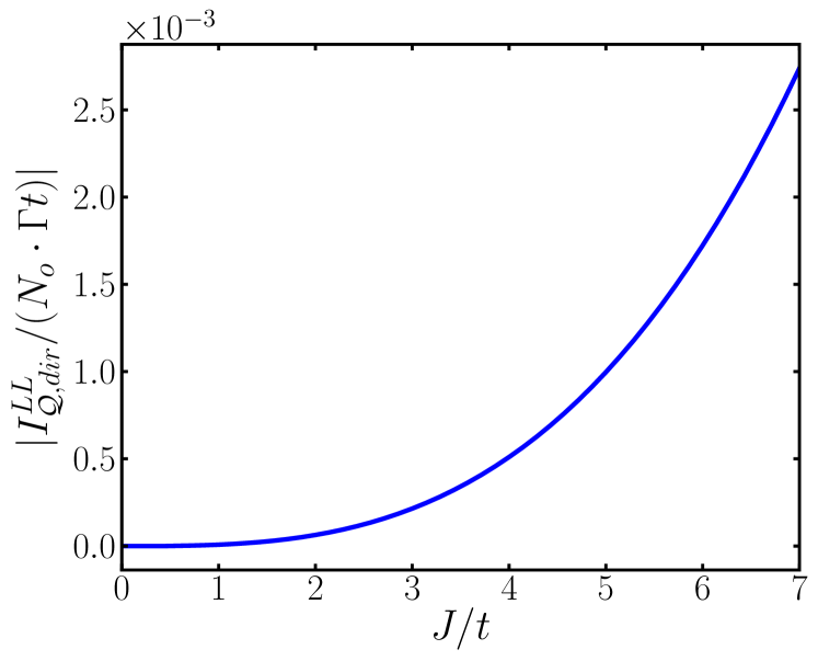
Figure 14: Dependence of $I^{LL}_{\bm{\mathcal{Q}},\text{dir}\text{}}=2\langle\mathbf{S}^{L}\rangle\cdot\hat{\mathbf{J}}^{L}T^{L}_{\mathbf{S}}$ on the Stoner splitting $J/t$, where $N_{o}$ is the fixed number of orbital states of the left subsystem and $J=5t$, $D=25t$, $T=t/2$.

The exchange SQM current, in contrast, shows a stronger dependence on the scalar parameters. To see this, we first roughly estimate how its emission and torque coefficients scale with $V$ and $J$ for low temperatures $T\lesssim V,J$. For $T=0$ the integrand of (107) is the product of the anisotropy function $a^{LL}(\omega)$, which has a support of width $2J$, and the bias function $\Delta(\omega)$ with a support of width $V$, and the smaller one of these energy scales limits the SQM emission:

$$E_{\mathrm{ex}}^{L} \approx -\frac{\Gamma}{2}\min(|V|,|J|),$$ (126)

where $\Gamma=2\pi|t|^{2}/(2D)^{2}$. In contrast, the SQM torque (109) scales in the same way as the spin torque:

$$T_{\mathrm{ex}}^{L} \approx -\frac{\Gamma}{\pi}\frac{J^{2}}{D},$$ (127)

where we also set $T=0$ and proceeded analogous to the estimation of the spin torque (cf. Eq. (124)). The additional suppression factor $J/D$ in Eq. (127) relative to Eq. (126) for $V<J$ reflects that the SQM torque originates from coherent virtual fluctuations to states near the band edges where the spin-polarization is nonzero in an energy window proportional to the Stoner splitting $J$. This gives rise to two regimes, in which the coherent exchange term (127) is larger (smaller) than the dissipative exchange term (126) for $V\lessgtr V^{\ast}$, where $E_{\mathrm{ex}}^{L}\sim T^{L}_{\mathrm{ex}}$ occurs for

$$V^{\ast} = \frac{J^{2}}{\pi D}.$$ (128)

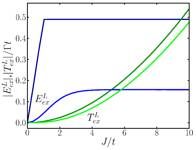
Figure 15: Dependence of the magnitude of SQM emission $|E^{L}_{\mathrm{ex}}|\text{/}\Gamma t$ (blue) and torque $|T_{\mathrm{ex}}^{L}|\text{/}\Gamma t$ (green) on the Stoner splitting  $J/t$ for $T=0$ (dark colors) and $T=0.5t$ (light colors). The residual parameters are $V=t$, $D=25t$. For $T=0$, the crossover occurs at $J\sim J^{\ast}=\sqrt{\pi DV\text{}}\approx 9t$. The initial non-linearity of the SQM emission coefficient for the finite temperature (preceded by a linear regime), and the smaller saturation value compared to the $T=0$ case are due to the thermal smearing.

Stoner-field dependence

In Fig. 15 we show a numerical calculation of the precise shapes (107) and (109) of the exchange emission coefficient $E_{\mathrm{ex}}^{L}$ and the torque coefficient $T_{\mathrm{ex}}^{L}$, confirming the estimates (126) and (127): they show that the torque increases quadratically and the emission saturates to a constant on the scale of bias $V$ (which is smaller than the value predicted by Eq. (126) due to finite temperature).

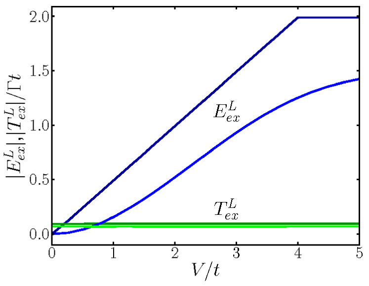
Figure 16: Dependence of the magnitude of SQM emission $|E_{\mathrm{ex}}^{L}|/\Gamma t$ (blue) and torque $|T_{\mathrm{ex}}^{L}|/\Gamma t$ (green) on the bias voltage $V/t$ for $T=0$ (dark colors) and $T=0.5t$ (light colors). The residual parameters are $J=5t$, $D=25t$. For both temperatures, the torque is constant at $|T^{L}_{\mathrm{ex}}|\approx 0.15$ according to estimation (127). The small deviation of this value and the saturation level of $|E_{\mathrm{ex}}^{L}|/\Gamma t$ for finite temperature compared to $T=0$ is due to the thermal smearing. Therefore, the rough estimate $V^{\ast}\approx J^{2}/\pi D\approx 1/3$ for the crossing point at $E_{\mathrm{ex}}^{L}=T^{L}_{\mathrm{ex}}$ is exactly fulfilled only for $T=0$.

Bias dependence

Fig. 16 shows the same crossover, but now as function of the bias $V$ for fixed $J$ and $T$. The torque is constant and given approximately by (127) and the emission saturates at the value set by (126) when $V$ approaches the scale of $J$. This  voltage dependence allows for magnetic and electric control over the orientation of the exchange SQM current tensor, discussed in the next Sec. V.2.3. The saturation at $V\sim J$ is an interesting, new feature of the dissipative exchange SQM current, not present in the charge or spin current. It provides access to the Stoner shift of the DOS, cf. Fig. 7, even without spin-polarization of the DOS in the bias window. Similar to the spin current a finite coherent SQM term remains at zero bias, even though the dissipative SQM current vanishes.

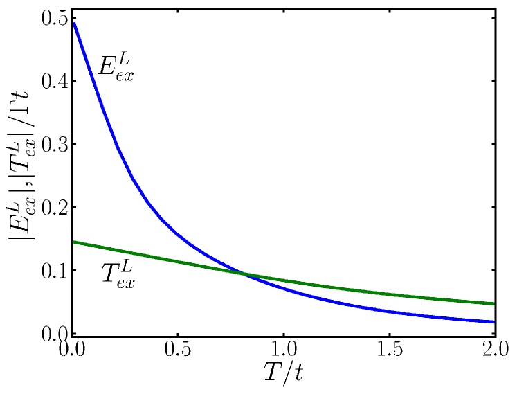
Figure 17: Dependence of the magnitude of exchange SQM emission $|E_{\mathrm{ex}}^{L}|/\Gamma t$ (blue) and torque $|T^{L}_{\mathrm{ex}}|/\Gamma t$ (green) on temperature $T/t$ for $V=t$, $J=5t$ $D=25t$.

Temperature dependence

In Fig. 17 we show the temperature dependence of the exchange SQM emission and torque coefficients, keeping $V$ and $J$ fixed. Both coefficients decrease monotonously with temperature, but with very different characteristic dependencies on $T$. The reason is that the emission integral (107) incorporates Fermi functions, which have a much stronger exponential dependence with $T^{-1}$, whereas torque integral (109) comprises the renormalization function $\beta^{R}$, which depends much weaker, namely algebraically on $T^{-1}$. Moreover, Fig. 17 shows that exchange SQM emission is strongly suppressed when $T$ approaches the voltage $V(<J)$ when the bias function $\Delta=f^{R}_{+}-f_{+}^{L}$ is largely broadened over an energy range of $\sim 4T\sim J$ (for the parameters of Fig. 17), so that positive and negative contributions of the spin-anisotropy function $a^{L}$ cancel each other. This is similar to the discussion of the exchange SQM storage in Sec. III.2.5.

V.2.3 Angle Dependence

The exchange SQM current, in contrast to the direct part, has a nontrivial dependence on the angle between the two Stoner vectors $\hat{\mathbf{J}}^{L}$ and $\hat{\mathbf{J}}^{R}$ due to the interplay of its dissipative and coherent contributions (see Sec. V.2.3). This requires a more extensive analysis since we are dealing with a tensor-valued current. There are two relevant questions relating to the orientation of the SQM tensors. The first question is whether the orientation of the local SQM $\langle\bm{\mathcal{Q}}^{LL}\rangle$ is changed by the injected SQM current $\langle\bm{\mathcal{I}}_{\bm{\mathcal{Q}}}^{LL}\rangle$. One can show that if these tensors commute, $[\langle\bm{\mathcal{I}}_{\bm{\mathcal{Q}}}^{LL}\rangle,\langle\bm{\mathcal{Q}}^{LL}\rangle]=0$, then the SQM current corresponds only to a change in the principal values of the local SQM without changing its principal axes (see App. C). Now Eq. (98) shows that for non-collinear $\widehat{\mathbf{J}}^{L}$ and $\widehat{\mathbf{J}}^{R}$  the average SQM current $\langle\bm{\mathcal{I}}_{\bm{\mathcal{Q}}}^{LL}\rangle$ is a superposition of three linearly independent, symmetric and traceless tensors, $\widehat{\mathbf{J}}^{L}\odot\widehat{\mathbf{J}}^{L}$ (emission (107)) , $\widehat{\mathbf{J}}^{L}\odot\widehat{\mathbf{J}}^{R}$(absorption (108)) and $\widehat{\mathbf{J}}^{L}\odot(\hat{\mathbf{J}}^{L}\times\widehat{\mathbf{J}}^{R})$ (torque (109)). The latter two tensors do not commute with $\langle\bm{\mathcal{Q}}^{LL}\rangle\propto\widehat{\mathbf{J}}^{L}\odot\widehat{\mathbf{J}}^{L}$ for non-collinear $\widehat{\mathbf{J}}^{L}$ and $\widehat{\mathbf{J}}^{R}$ and vanish only for collinear $\widehat{\mathbf{J}}^{L}$ and $\widehat{\mathbf{J}}^{R}$. This holds for both the direct and exchange contributions. Therefore the injected average SQM current $\langle\bm{\mathcal{I}}_{\bm{\mathcal{Q}}}^{LL}\rangle$ will tend to change the principal axes of the average local SQM $\langle\bm{\mathcal{Q}}^{LL}\rangle$, besides changing its principal values.

The second question is whether the direct and exchange SQM currents tend to induce the same rotation of the principal axis of the SQM, which is equivalent to these tensors commuting, $[\langle\bm{\mathcal{I}}_{\bm{\mathcal{Q}}}^{LL}\rangle_{\mathrm{dir}},\langle\bm{\mathcal{I}}_{\bm{\mathcal{Q}}}^{LL}\rangle_{\mathrm{ex}}]=0$. To show that this is not the case, we now first explicitly find the (different) principal axes and values of $\langle\bm{\mathcal{I}}^{LL}_{\bm{\mathcal{Q}}}\rangle_{\mathrm{dir}}$ and $\langle\bm{\mathcal{I}}^{LL}_{\bm{\mathcal{Q}}}\rangle_{\mathrm{ex}}$. This will furthermore allow us to plot and discuss these average SQM currents in a clear way.

Principal axes and values

The following analysis holds for any dispersion $\varepsilon^{r}_{nk\sigma}$. We first diagonalize the full average SQM current tensor Eq. (98) and then show how the direct and exchange part can be obtained from the result. Since the former is real and symmetric tensor it can always be diagonalized:

$$\langle\bm{\mathcal{I}}^{LL}_{\bm{\mathcal{Q}}}\rangle = \sum_{\lambda=\pm,0}I_{\lambda}\hat{\mathbf{v}}_{\lambda}\hat{\mathbf{v}}_{\lambda}.$$ (129)

Here the $\hat{\mathbf{v}}_{\lambda}$ denote the orthonormal principal axes (the hat indicating normalization) and the $I_{\lambda}$ denote principal SQM currents, which quantify the magnitude of the SQM current. (We dropped the superscripts “$LL$” on $I_{\lambda}$ and $\hat{\mathbf{v}}_{\lambda}$ for brevity). In App. B we show that for non-collinear Stoner vectors ($\cos(\theta)=\widehat{\mathbf{J}}^{L}\cdot\widehat{\mathbf{J}}^{R}\neq\pm 1$) the principal SQM currents are

$$I_{0} = -\tfrac{1}{3}D_{\theta},$$ (130)

$$I_{\pm} = \tfrac{1}{6}D_{\theta}\pm\tfrac{1}{2}S_{\theta},$$ (131)

which add up to 0 as they should (traceless tensor). The unnormalized principal axes read

$$\mathbf{v}_{0} = \widehat{\mathbf{J}}^{L}\times\left(A_{\bm{\mathcal{Q}}}^{L}\widehat{\mathbf{J}}^{R}+T^{L}_{\bm{\mathcal{Q}}}\widehat{\mathbf{J}}^{L}\times\widehat{\mathbf{J}}^{R}\right),$$ (132)

$$\mathbf{v}_{\pm} = (D_{\theta}\pm S_{\theta})\widehat{\mathbf{J}}^{L}+A^{L}_{\bm{\mathcal{Q}}}\widehat{\mathbf{J}}^{R}+T^{L}_{\bm{\mathcal{Q}}}\widehat{\mathbf{J}}^{L}\times\widehat{\mathbf{J}}^{R}.$$ (133)

In Eqs. (130)-(133), we used the abbreviations

$$D_{\theta} := \left(E^{L}_{\bm{\mathcal{Q}}}+A^{L}_{\bm{\mathcal{Q}}}\cos\theta\right),$$ (134)

$$S_{\theta} := \sqrt{D_{\theta}^{2}+\left(\left(T^{L}_{\bm{\mathcal{Q}}}\right)^{2}+\left(A^{L}_{\bm{\mathcal{Q}}}\right)^{2}\right)\sin^{2}\theta}.$$ (135)

The principal SQM currents obey the inequalities

$$I_{-}\leqslant I_{0}\leqslant I_{+}$$ (136)

since $S_{\theta}\geqslant D_{\theta}$. For collinear Stoner vectors ($\theta=0,\pi$), two eigenvalues are degenerate,

$$I_{+} = \left(\tfrac{p}{6}+\tfrac{1}{2}\right)\left|E^{L}_{\bm{\mathcal{Q}}}+A^{L}_{\bm{\mathcal{Q}}}\right|,$$ (137)

$$I_{-} = \left(\tfrac{p}{6}-\tfrac{1}{2}\right)\left|E^{L}_{\bm{\mathcal{Q}}}+A^{L}_{\bm{\mathcal{Q}}}\right|,$$ (138)

$$I_{0} = \tfrac{p}{3}\left|E^{L}_{\bm{\mathcal{Q}}}+A^{L}_{\bm{\mathcal{Q}}}\right|$$ (139)

with $p=\mathrm{sgn}(D_{0})$, $\hat{\mathbf{v}}_{+}=\hat{\mathbf{J}}^{L}$ and any two vectors in the plane perpendicular to $\hat{\mathbf{J}}^{L}$ are principal axes of the SQM current. We thus see that in general, the principal SQM currents take three different values, i.e. a bi-axial spin-anisotropy is transported whenever the Stoner vectors are non-collinear. We emphasize that by itself the average spin-current vector provides no information about the non-collinearity of the spin-valve. The SQM current tensor, in contrast, does: the transported anisotropy only becomes uniaxial for collinear Stoner vectors ($\theta=0,\pi$), in which case $\hat{\mathbf{J}}^{L}$ is the hard axis. The possibility of injecting biaxial anisotropy into molecular scale systems is of interest since this type of anisotropy it is associated with interesting quantum-spin tunneling effects Gatteschi and Sessoli (2003).

We obtain the diagonal form of the direct and exchange SQM individually by replacing the coefficients Eq. (116)-(118) in the above formulas by $E^{L}_{\bm{\mathcal{Q}}}\rightarrow E^{L}_{\text{dir}}=\left(\mathbf{S}^{L}\cdot\widehat{\mathbf{J}}^{L}\right)E^{L}_{\mathbf{S}}$ and $E^{L}_{\bm{\mathcal{Q}}}\rightarrow-E^{L}_{\mathrm{ex}}$, respectively, etc. Since these two sets of coefficients are in general different functions of the various parameters, we conclude that the direct and exchange SQM tensors have different principal axes and do not commute, $[\langle\bm{\mathcal{I}}_{\bm{\mathcal{Q}}}^{LL}\rangle_{\mathrm{dir}},\langle\bm{\mathcal{I}}_{\bm{\mathcal{Q}}}^{LL}\rangle_{\mathrm{ex}}]\neq 0$. They therefore tend to induce the different rotations of the principal axis of the local SQM.  As a result the total principal SQM currents are not the sum of the direct and exchange principal SQM currents.

Flat band approximation

So far the considerations were general. We now investigate the magnetic tuning of the exchange SQM orientation by the Stoner vectors. For the flat band approximation, Eq. (119)-(121), the principal SQM currents and the principal axes are symmetric with respect to $\theta=\pi/2$, i. e.,

$$I_{\lambda}\left(\tfrac{\pi}{2}-\alpha\right) = I_{\lambda}\left(\tfrac{\pi}{2}+\alpha\right),$$ (140)

$$\hat{\mathbf{v}}_{\lambda}\left(\tfrac{\pi}{2}-\alpha\right) = \hat{\mathbf{v}}_{\lambda}\left(\tfrac{\pi}{2}+\alpha\right).$$ (141)

This is due to the vanishing SQM absorption coefficient, $A^{L}_{\bm{\mathcal{Q}}}$, in this limit. In Fig. 18 we plot both the direct and the exchange principal SQM currents as a function of the angle $\theta\in[0,\pi/2]$. We observe that both $I_{0}^{\mathrm{dir}}$ and $I_{0}^{\mathrm{ex}}$ are constant. In both cases, the repulsion of both  $I_{\pm}^{\mathrm{dir}/\mathrm{ex}}$ is caused by the respective torque coefficient (see Eq. (134)), which increases with $J$ and decreases with $D$ (cf. Eq. (124)-(127)).

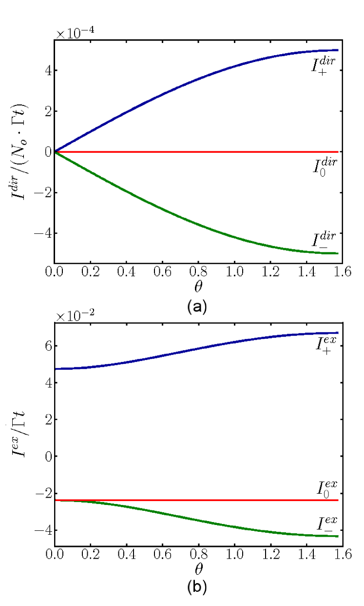
Figure 18: Angle dependence of the principal SQM currents (a) $I_{\lambda}^{\text{dir}}/(t\cdot N_{s})$ and (b) $I_{\lambda}^{\mathrm{ex}}/t$, respectively (red: $I_{0}$, green: $I_{-}$, blue: $I_{+}$). The principal direct SQM currents only depend on the nonzero spin torque $I_{\lambda}^{\mathrm{dir}}=\lambda 2|\mathbf{S}^{L}||T^{L}_{\mathbf{S}}\sin\theta|$ $(\lambda=0,\pm)$, whence the principal exchange SQM currents depend both the nonzero exchange SQM emission and torque. Parameters: $J=5T$, $D=25t,V=T=t$, $\Gamma=2\pi/2500$. Note that the inequalities Eq. (136) and $\sum_{\lambda}I_{\lambda}^{\mathrm{dir}}=\sum_{\lambda}I_{\lambda}^{\mathrm{ex}}=0$ are fulfilled.

To analyse the angle dependence of the principal axes $\hat{\mathbf{v}}_{\lambda}$, we construct a right handed coordinate system from the non-collinear, non-orthogonal Stoner vectors: let $\mathbf{e}_{z}=\widehat{\mathbf{J}}^{L}$, $\mathbf{e}_{x}=\widehat{\mathbf{J}}^{L}\times\widehat{\mathbf{J}}^{R}/\sin\theta$, $\mathbf{e}_{y}=\mathbf{e}_{z}\times\mathbf{e}_{x}$. In Fig. 19 we show the trajectories of the direct and exchange principal axes as we rotate $\widehat{\mathbf{J}}^{R}=-\sin\theta\mathbf{e}_{y}+\cos\theta\mathbf{e}_{z}$ through $\theta\in[0,\pi/2]$. Then both $\hat{\mathbf{v}}_{0}^{\text{dir}}=\hat{\mathbf{v}}^{\mathrm{ex}}_{0}=\mathbf{e}_{y}$ are a fixed directions in this coordinate system, i.e., independent of the angle $\theta$. The other principal axes $\hat{\mathbf{v}}_{\pm}^{\text{dir$/\mathrm{ex}$}}$ lie in the $xz$-plane perpendicular to $\hat{\mathbf{v}}^{\text{dir$/$ex}}_{0}$ and are different for the direct and exchange contribution.

The direct SQM current only consists of a torque contribution and therefore its principal axes are independent of $\theta$ in the above coordinate system fixed by $\widehat{\mathbf{J}}^{L}$ and $\widehat{\mathbf{J}}^{R}$. With $A^{L}_{\text{dir}}=E^{L}_{\text{dir}}=0$ and $T^{L}_{\text{dir}}=2(\mathbf{S}^{L}\cdot\widehat{\mathbf{J}}^{L})T^{L}_{\mathbf{S}}$, Eq. (132)-(133) give $\hat{\mathbf{v}}^{\text{dir}}_{\pm}=\left(\pm\mathbf{e}_{z}-\mathbf{e}_{x}\right)\text{/}\sqrt{2}$ for $\theta\neq 0,\pi$ (when the direct SQM current is nonzero). In contrast, the exchange SQM current shows a nontrivial competition of the torque and emission contributions: in Fig. 19 we plot the trajectories of its principal axes in the plane perpendicular to $\hat{\mathbf{v}}_{0}^{\mathrm{ex}}=\mathbf{e}_{y}$ as $\theta$ is increased to from 0 to $\pi/2$.

We emphasize that already in this simple model of flat-band ferromagnets the spin-anisotropy flow has non-trivial tensorial structure: in general the principal axes of the exchange SQM tensor are neither collinear to $\widehat{\mathbf{J}}^{L}$, $\widehat{\mathbf{J}}^{R}$ nor collinear to $\widehat{\mathbf{J}}^{L}\times\widehat{\mathbf{J}}^{R}$. Only for nearly collinear configurations ($\theta\approx 0,\pi$), when the torque contribution is negligible, do we have such a simple result: $\widehat{\mathbf{v}}_{+}^{\mathrm{ex}}\approx\mathbf{e}_{x}=\widehat{\mathbf{J}}^{L}$ and $\widehat{\mathbf{v}}_{-}\approx\mathbf{e}_{z}=\widehat{\mathbf{J}}^{L}\times\widehat{\mathbf{J}}^{R}\text{/}\sin(\theta)$.

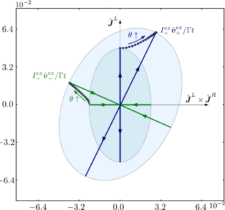
Figure 19: Angle dependence of the exchange SQM tensor $\langle\bm{\mathcal{I}}_{\bm{\mathcal{Q}}}^{LL}\rangle_{\mathrm{ex}}$. Each point corresponds an principal vector $I^{\mathrm{ex}}_{+}\hat{\mathbf{v}}^{\mathrm{ex}}_{+}/t$ (blue) and $I^{\mathrm{ex}}_{-}\hat{\mathbf{v}}_{-}^{\mathrm{ex}}/t$ (green) of $\langle\bm{\mathcal{I}}_{\bm{\mathcal{Q}}}^{LL}\rangle_{\mathrm{ex}}$ for increasing angle $\theta$ in steps of $\pi/36$ from $0$ to $\pi/2$. Each pair of vectors $I^{\mathrm{ex}}_{\pm}\hat{\mathbf{v}}_{\pm}^{\mathrm{ex}}/t$ for one angle defines the semi axes of an ellipse, drawn for the extremal values $\theta=0$ and $\theta=\pi/2$. The axes of this ellipse indicate the principal axes of $\langle\bm{\mathcal{I}}_{\bm{\mathcal{Q}}}^{LL}\rangle_{\mathrm{ex}}$ and and the diameter $2|I_{\pm}/t|$ gives the principal SQM currents. The arrows of the semi axes indicate the sign of the principal SQM current: it is positive (negative) if the arrow points away from (towards) the origin. The full tensor can be visualized by including the principal vector $I^{\mathrm{ex}}_{0}\hat{\mathbf{v}}^{\mathrm{ex}}_{0}/t\propto\mathbf{e}_{y}$ (pointing into the plane), completing the ellipse to an ellipsoid. $\hat{\mathbf{J}}^{R}$ is rotated from $\hat{\mathbf{J}}^{L}$ $(\theta=0)$ out of the plane when $\theta$ increases. The residual parameters are $D=25T$, $J=5T$ , $V=T=t$,  $\Gamma=2\pi/2500$.

A further striking property of the exchange principal axes is that they can not only be tuned magnetically by the Stoner vectors but also to a large extent electrically. As discussed in Sec. V.2.2 there is a crossover, shown in Fig. 16, from a torque-dominated (low bias) to an emission-dominated exchange SQM (large bias). As a result, increasing the voltage results in a change of the principal axes of the SQM current - an effect that is comparable to that resulting from tuning the angle $\theta$ between the magnetizations in Fig. 19.

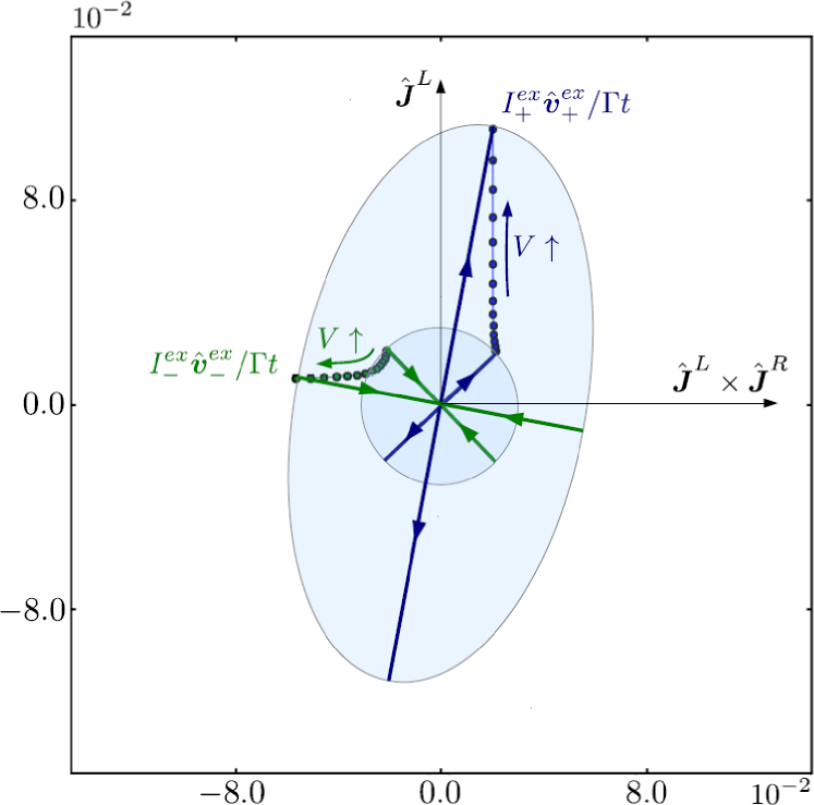
Figure 20: Voltage dependence of the exchange SQM tensor. For explanation see Fig. 19 where each points corresponds to a a different voltage $V/t$, increasing in steps of $1/10$ from $0$ to $1.5$. The remaining parameters are $\theta=\pi/4$, $D=25T$, $J^{L}=J^{R}=5t$ , $T=t$, $\Gamma=2\pi/2500$.

The voltage scale at which the direct and exchange SQM current compete, i.e., $|E^{L}_{\mathrm{ex}}|\sim|T^{L}_{\mathrm{dir}}|=2|\mathbf{S}^{L}|T_{\mathbf{S}}^{L}$, can be estimated using $|\mathbf{S}^{L}|\sim JN_{o}/D\sim N_{s}$ (cf. Eq. (27)) to

$$V \sim (J^{2}/D)N_{s}.$$ (142)

Since by Eq. (126) $E^{L}_{\mathrm{ex}}$ has a voltage dependence only for $V\lesssim J$, the electric tuneability is feasible only when the crossover scale (142)  $\lesssim$ $J$: this is the case when the number of polarized spin $N_{s}\lesssim D/J$, i. e. the number of orbitals is limited to $N_{o}\lesssim(D\text{/}J)^{2}$, which can still be fairly large number. This is a first indication that for mesoscopic ferromagnets this electrical tuneability of the SQM orientation may be possible and may be an interesting topic for future analysis. We emphasize the crudeness of our model here and the importance of investigating charging and non-equilibrium effects, see Ref. Hell and Wegewijs (2013).

V.3 Transport of spin anisotropy without spin current

Finally, we explore the possibility of a pure spin-anisotropy current, i. e. a non-vanishing SQM current in the absence of  a spin current, which was anticipated in Sec. V.1.3.

V.3.1 Conditions for zero charge and spin current

We first discuss the conditions for a vanishing spin current for a general band structure $\varepsilon^{r}_{nk\sigma}$. We expect zero spin current only for collinear magnetizations. If the magnetizations are non-collinear, the spin current has three non-collinear contributions and demanding that all these vanish requires $E_{\mathbf{S}}^{L}=A_{\mathbf{S}}^{L}=T_{\mathbf{S}}^{L}=0$. This might be possible, but only for special band structures and parameter values ($T^{r},\mu^{r}$), but this is beyond the scope of this paper. For collinear magnetizations, the spin torque automatically vanishes and the spin current reads $\langle\mathbf{I}_{\mathbf{S}}\rangle=\int\mathrm{d}\omega\Gamma\Delta\left(n^{L}\hat{\mathbf{J}}^{L}+n^{R}\hat{\mathbf{J}}^{R}\right)$ with $\widehat{\mathbf{J}}^{L}||\widehat{\mathbf{J}}^{R}$. A generic situation with cancelling spin current is then given for antiparallel magnetized ($\widehat{\mathbf{J}}^{L}=-\widehat{\mathbf{J}}^{R}$) ferromagnets with identical spin-polarization of the 1DOS in the bias window, that is, $n^{L}(\omega)=n^{R}(\omega)$, so that the bracket in the above integrand is zero. This defines a parameter regime for which $\langle\mathbf{I}_{\mathbf{S}}\rangle=0$, as one may still apply any voltage or temperature bias. Again, there might be exotic material combinations, for which the spin current even vanishes for $\widehat{\mathbf{J}}^{L}=+\widehat{\mathbf{J}}^{R}$. For our crude flat band approximation (cf. Sect. II.4), the dissipative spin current is zero in any case, so that collinearity $\widehat{\mathbf{J}}=\widehat{\mathbf{J}}^{L}=\pm\widehat{\mathbf{J}}^{R}$ of the Stoner vectors is already sufficient for cancelling spin current.

We can even go one step further and envisage a situation, for which the charge current vanishes as well: note that it still has a non-magnetic contribution (100) $\propto\int\mathrm{d}\omega\Delta$ ($\Gamma$ is constant in the bias window and we consider $T^{r}\ll D$). For pure voltage bias $\mu^{L}\neq\mu^{R}$, but $T^{L}=T^{R}$, the bias function $\Delta(\omega)$ is symmetric and positive and we will always have a charge current. However, for a pure temperature bias, $T^{L}\neq T^{R}$ and $\mu^{L}=\mu^{R}$, the bias function $\Delta=f^{R}_{+}-f^{L}_{+}$ is antisymmetric and the charge current contributions above and below the common electrochemical potential cancel. Since $T^{R}>T^{L}$ the right “hot” electrode has a larger (smaller) occupation probability for electrons with energy $\omega>\mu$ ($\omega<\mu$) than the left electrode. Consequently, the particle current flowing from left to right for electrons with energy $\omega>\mu$ exactly cancels the charge current for electrons flowing from the right to the left at energies $\omega<\mu$. Integrated over all frequencies this gives the zero net charge current.

V.3.2 Pure quadrupole current

Strikingly, in contrast to charge and spin current, the SQM current remains non-zero for a pure thermal bias. It comes entirely from the exchange emission part:

$$\langle\bm{\mathcal{I}}^{LL}_{\bm{\mathcal{Q}}}\rangle = -2\Gamma\int\mathrm{d}\omega\Delta a^{L}\widehat{\mathbf{J}}\odot\widehat{\mathbf{J}}\neq 0,$$ (143)

where $\Gamma$ can be pulled out of the integral since the DOS is constant at energies $\omega$ for which $a^{L}(\omega)\neq 0$. Since the spin-anisotropy function $a^{L}(\omega)$, Eq. (68), is antisymmetric as well we integrate an overall symmetric function and $\langle\bm{\mathcal{I}}^{LL}_{\bm{\mathcal{Q}}}\rangle$ is non-zero. This is a central result of the paper. In Fig. 21 we plot the total SQM current for a thermal bias with collinear Stoner vectors as function of the temperature difference, as given by Eq. (143). In Fig. 22 we plot the dependence on the Stoner field $J^{L}$.

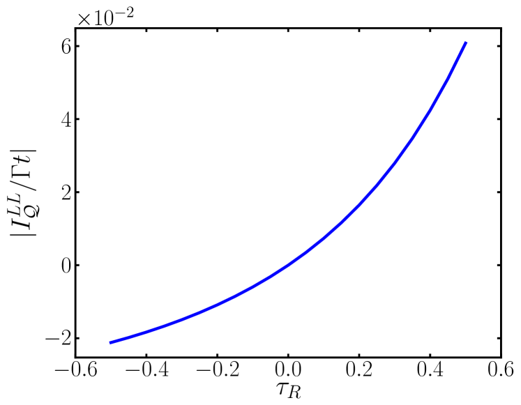
Figure 21: $\left|I_{\bm{\mathcal{Q}}}^{LL}\right|/t$ (from Eq. (143) with $\langle\bm{\mathcal{I}}^{LL}_{\bm{\mathcal{Q}}}\rangle=-I_{\bm{\mathcal{Q}}}^{LL}\widehat{\mathbf{J}}\odot\widehat{\mathbf{J}}$ as a function of the temperature bias ratio $\tau^{R}=(T^{R}-T^{L})/T^{R}$ for $T^{L}=t$, $J=5t$, $D=25t$ and $\Gamma=2\pi/2500$.

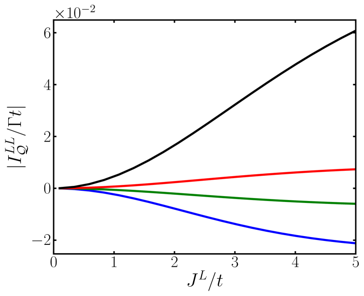
Figure 22: Same as Fig. 21, but now showing $\left|I_{\bm{\mathcal{Q}}}^{LL}\right|/t$ as function of Stoner splitting $J^{L}/t$ for fixed thermal bias $\tau^{R}=(T^{R}-T^{L})/T^{R}=-0.5,-0.1,0.1,0.5$ (from topmost to bottommost curve). The antisymmetry of the linear result Eq. (144), $I_{\bm{\mathcal{Q}}}^{LL}(\tau_{R})\approx I_{\bm{\mathcal{Q}}}^{LL}(-\tau_{R})$, breaks down in the non-linear regime as shown in  as Fig. 22 for $\tau_{R}=\pm 0.5$.

The linear response in the temperature bias ratio $\tau^{R}=(T^{R}-T^{L})/T^{R}\ll 1$ varied for fixed $T^{L}$ gives for the SQM current magnitude, defined here by $\langle\bm{\mathcal{I}}^{LL}_{\bm{\mathcal{Q}}}\rangle=-I^{LL}_{\bm{\mathcal{Q}}}\widehat{\mathbf{J}}\odot\widehat{\mathbf{J}},$

$$I_{\bm{\mathcal{Q}}}^{LL} = \frac{\Gamma}{2}(T^{L}-T^{R})\times$$ (144)

$$\frac{T^{L}}{T^{R}}\left[1-\left(\frac{J^{L}/2T^{L}}{\sinh(J^{L}/2T^{L})}\right)^{2}\right].$$

For fixed, different temperatures, the magnitude of the SQM current increases monotonously as a function of the Stoner splitting as shown in Fig. 22. It eventually saturates for $J^{L}\approx 10T^{L}$ at the asymptotic value of $I_{\bm{\mathcal{Q}}}^{LL}\approx(\Gamma\text{/2})\tau^{R}T^{L}$.

A crude understanding of the above results is the following. Since the magnitude of local exchange SQM decreases with temperature (Pauli exclusion effects get washed out thermally), cf. Fig. 9 and Eq. (72), the thermal gradient induces a “gradient in the correlations” resulting in the SQM flow of Pauli exlusion holes from the colder to the hotter reservoir, roughly speaking.

We emphasize, however, that this should not be interpreted as a direct transfer of spin-correlations between the two local SQM nodes since they first have to be converted into non-local spin-correlations: in the language of our network picture, these are first buffered in the non-local intermediate node. This becomes clearer in view of the SQM conservation law (95), which reads of our device (cf. Fig. 12) after averaging $\langle\bm{\mathcal{I}}^{LR}_{\bm{\mathcal{Q}}}\rangle=-\langle\bm{\mathcal{I}}^{LL}_{\bm{\mathcal{Q}}}\rangle-\langle\bm{\mathcal{I}}^{RR}_{\bm{\mathcal{Q}}}\rangle$. Interchanging the role of the left and the right electrode in Eq. (144), we see that the change in the local spin-anisotropy of the $\langle LL\rangle$- and $\langle RR\rangle$-node have opposite sign. Taking only the $O(\Delta T)$- contribution, we may replace $T^{L}$ and $T^{R}$, respectively, by the average temperature in the second line of Eq. (144): we then find that there is no net creation of non-local spin-correlations only to first order in in the thermal bias $\Delta T$, i. e., $\langle\bm{\mathcal{I}}^{LR}_{\bm{\mathcal{Q}}}\rangle=O(\Delta T^{2})$.

A more rigorous explanation of the thermally driven SQM current is based on a microscopic point of view (cf. Secs. III.2.4 and III.2.5). These considerations may be useful for proposals for more complicated device setups that would allow for the detection a pure SQM current (an issue that is not covered here). The exchange SQM in (143) is quantified by the anisotropy function $a^{L}(\omega)$ (cf. Eq. (68) and Fig. 7), which describes the Pauli exclusion hole to which an electron at energy $\omega$ contributes. The microscopic reason why $a^{L}(\omega)$ changes sign was explained in detail in Sec. III.2.5: basically for $\omega<\mu$ ($\omega>\mu$) a given electron at energy $\omega$ most likely sees a parallel (antiparallel) spin at energy $\omega+J$ ($\omega-J$). Electrons with opposite energies relative to $\mu$ thus contribute with an opposite sign to the Pauli exclusion hole. Since the thermal bias transports electrons above and below the Fermi edge into opposite directions, the contributions to the local average SQM $\langle\bm{\mathcal{Q}}^{LL}\rangle$ thus add up, explaining why Eq. (143) is finite. Notably, the thermal bias drives this flow of spin correlations between the ferromagnets without any other one-particle quantity being net transported. For example, the charge of each electron is independent of its energy and therefore the contributions above and below the Fermi energy cancel.

Importantly, in this case the direction of the spin-anisotropy flow can be controlled by the sign of the temperature gradient: for $T^{L}<T^{R}$, the SQM current magnitude $I^{LL}_{\bm{\mathcal{Q}}}$ is negative, i. e., local planar spin-triplet correlations are net delocalized by the tunneling. The left local node therefore loses Pauli exclusion holes. This can be understood following arguments similar to that of the purely voltage-biased tunnel junction (see Sect. V.2.1). However, in stark contrast to pure voltage bias, the current magnitude $I^{LL}_{\bm{\mathcal{Q}}}$ becomes positive if $T^{R}<T^{L}$. This physically means that net local planar spin-correlations are created by tunneling. The reason is that electrons are injected into the left electrode below the Fermi energy. As these electron obey Pauli’s principle, they are forced to form new Pauli-exclusion holes. Furthermore, the electrons are extracted only above the Fermi energy and they carry away positive (axial) spin correlations (leaving a negative contribution behind). For the contrasting situation of a pure voltage bias, the energy-resolved flow direction has to be opposite: electrons care only net injected (extracted) at energies larger (lower) then the Fermi energy.

As a conclusion, the possibility to control the spin-anisotropy flow direction by the thermal bias applied to the tunnel junction is a non-trivial result of this paper. This fact and the prediction of a pure spin-quadrupole moment current demonstrate most clearly that triplet-spin correlations form an independent degree of freedom which is not only stored in a system of ferromagnets, but can also be transported between them.

VI Summary and Outlook

In this paper we investigated fundamental questions about the spin anisotropy, as quantified by the spin-quadrupole moment (SQM), which arise when it is considered as a transport quantity. In the physical language of atomic and molecular magnetism, the SQM characterizes the quadratic spin anisotropy, which is usually its dominant part. It quantifies the preference of spins to be aligned along a specific axis irrespective of their orientation along it (up, down). We addressed three central questions related to the quantum transport of spin-anisotropy: (i) how can SQM be stored in and (ii) transported between two ferromagnets in a spintronic circuit; (iii) how can one define an SQM current tensor operator, derive SQM continuity equations and SQM current conservation laws; how does the non-equilibrium steady-state average of the SQM current relate to the spin-current?

Our work was motivated by studies Sothmann and König (2010); Baumgärtel et al. (2011); Misiorny et al. (2012a) that indicated that the physical picture of the transport of spin degrees of freedom through magnetic nanostructures needs to be extended. A refinement of this picture, resulting from this paper, is as follows. Electrons are charged particles with an intrinsic spin-dipole moment and vanishing higher spin moments. Therefore, the motion of an isolated electron is associated with a charge and spin current only. However, in a multi-electron system the electron becomes correlated with other electrons. Moving this electron therefore implies a change of correlations. In particular, the transfer of spin-triplet correlations between different subsystems is quantified by the spin-quadrupole current. This complements the results of prior studies Sothmann and König (2010); Baumgärtel et al. (2011); Misiorny et al. (2012a), which demonstrated that these tensor-valued currents lead to an accumulation of SQM. The latter couples to the accumulation of spin and charge and their measurable currents. In this paper we ignored the complications of this accumulation, as well as interaction and non-equilibrium effects that appear in nanoscale spintronic devices. We exclusively focused on the description of transort of SQM between macro- and mesoscopic circuit elements.

Answering question (i), we found that macroscopic ferromagnets, the basic elements of spintronic devices, store a macroscopic SQM, which is generated by their internal Stoner field. This direct spin-anisotropy is of easy-axis type and scales quadratically with the number of half-filled, spin-polarized orbitals $N_{s}$. This follows the classical intuition that orientation of spins also implies their alignment. However, for mesoscopic systems, an additional quantum exchange contribution to the SQM becomes relevant Misiorny et al. (2012a), which scales linearly with $N_{s}$. It quantifies the effect of Pauli-exclusion holes that exist in the triplet two-particle spin correlations, expressing the simple fact that electrons in the same orbital do not form a triplet spin state. This Pauli-forbidden spin-anisotropy is of the easy-plane type, countering therefore the direct easy-axis anisotropy.

Importantly, the effect of the Pauli exclusion holes is cumulative, i. e., their contributions always add up and cannot cancel each other. This is in stark contrast to the average spin-dipole moment, for which contributions from electrons with opposite spin orientation can cancel each other. This shows that the average SQM is a degree of freedom independent of one-particle quantities such as average charge and spin.

To answer question (ii) we developed a spin-multipole transport theory with an associated network picture. For spin-dipole moment, each ferromagnet is represented by a node of the network storing spin-dipole moment. However, due to its two-particle nature in electronic systems, SQM is also stored as non-local correlations between spins from different spin-polarized subsystems. The network picture of SQM therefore incorporates also non-local SQM nodes. As a consequence, the  SQM network differs from the physical layout of the system of ferromagnets, both in the number of nodes and in their connectivity. For the two-terminal spin-valve that we studied in this paper, this network thus consists of three SQM nodes. This network theory also applies also to spin-valves with embedded quantum dots Hell and Wegewijs (2013).

Based on this microscopic picture, we  inferred the proper definition of the spin-quadrupole current tensor operators, answering question (iii). By a continuity equation, the SQM currents generate the change of the local anisotropy due to quantum transport processes. They furthermore obey a current conservation law expressing the conservation of SQM in the tunneling. For the two-terminal spin-valve it reads $\mathcal{I}^{LL}_{\mathcal{Q}}+\mathcal{I}^{RR}_{\mathcal{Q}}+\mathcal{I}^{LR}_{\mathcal{Q}}=0$.

Finally, we found by explicit calculation that the non-equilibrium steady-state average of all these these SQM currents is non-zero, even for this elementary spintronic setup and analysed these in detail. Similar to the average SQM, these average SQM currents have a decomposition into classical and quantum two-particle contributions, similar to the average SQM itself. The direct SQM current is implied by a non-zero average spin and spin current. It reflects the classical intuition that “orientation implies alignment”. In addition to this, we found an quantum exchange SQM current, which is profoundly different from spin currents.

In analogy to the spin, we also distinguished dissipative and coherent contributions to the SQM: the spin precession responsible for the spin-torque term in the spin-current – lifting the spin out of the plane of the Stoner vectors – has a counterpart in the SQM current. These spin-torque SQM terms similarly result from coherent fluctuations by virtual tunneling into a ferromagnet (i. e., spin-dependent scattering) which probe the spin-dependence of the entire band structure. This effect is also responsible for the exchange field J. König and J. Martinek (2003) in quantum dot spin-valves. The different bias-voltage dependence of the dissipative and coherent terms allows for electric control of both the magnitude and the orientation of the spin-anisotropy current tensor.

Furthermore, for non-collinear ferromagnets, the spin-anisotropy current was found to be a bi-axial tensor. Its three distinct principal values and axes reflect the lowered symmetry of a non-collinear setup, which is not revealed by the spin current, which is just a vector. We showed that this dependence on the Stoner vectors allows for substantial magnetic tuning of the SQM current tensor orientation. The possibility of injecting biaxial anisotropy into, e.g., molecular magnets is of interest since the intrinsic, spin-orbit generated anisotropy of this type is associated with quantum-spin tunneling effects Gatteschi and Sessoli (2003).

The striking central result of this paper, as announced by the paper title, is a pure SQM current whenever the spin current vanishes by net cancellation of one-particle contributions. This spin-anisotropy flow is  driven by a gradient of Pauli exclusion holes in the triplet spin-spin correlations, that is, a true quantum two-particle current. We illustrated this general result for a temperature-biased junction connecting two anti-parallel ferromagnets with a flat-band DOS. In this case, a pure SQM current generates an uniaxial, easy plane anisotropy, i.e., a negative anisotropy that counteract an easy axis anisotropy. It may be of interest to inject such an SQM current into a single-molecule magnet considered as a memory cell in order to temporarily switch off its easy-axis anisotropy barrier in order to put it into “writing” mode. This also relates to the recently studied tunnel-induced renormalization of the intrinsic anisotropy of molecular magnets in contact with spin-polarized electrodes Misiorny et al. (2011); May et al. (2011); Misiorny et al. (2012a). One may even envisage the utilization of SQM as a resource, as an alternative to conventional spintronics, i.e., utilize the storage, transport, manipulation and readout of spin anisotropy without transporting or affecting spin polarization. The possibility of pure SQM currents pointed out in this paper indicates that this is principle conceivable and warrants further study. Altogether the above indicates that the theory of a generalized “spin-multipoletronics”, is a real possibility, if not a necessity when spintronics moves to the nanoscale.

We acknowledge G. E. W. Bauer, M. Büttiker, D. P. DiVincenzo, J. König, M. Misiorny, R. Saptsov and J. Splettstösser for useful discussions.

Appendix A Storage of Spin-quadrupole Moment

In this appendix we give the calculation of the local average SQM stored in a ferromagnet, cf. Sec. III.2.3. We present three derivations, each of which unveils different physical and technical aspects used in the main part. The first, most straightforward approach is given in Sec. A.1. It shows how the Pauli exclusion hole arises in Eq. (150), which provides the key to the physical interpretation of exchange SQM. Secondly, we give a technically more sophisticated derivation in Sec. A.2, which will be helpful to understand all steps of our transport calculations. It expresses the Pauli exclusion hole in a coordinate-free form in Eq. (161). Thirdly, we present in Sec. A.3 a derivation that makes explicit the spin-triplet content of the correlations by vector coupling of the spins of electron pairs. Finally, we discuss the spin-anisotropy function and derive a closed expression for the exchange SQM in the flat band approximation (cf. II.4). Throughout the appendix we focus on understanding the exchange contributions to the SQM, which we showed in the absence of tunneling to appear only locally for $(r=r^{\prime})$, cf. III.2.3. We therefore only consider one electrode $r$ with one band $n$ and subsequently drop these indices in all expressions below, e. g. $c_{rnk\sigma}\rightarrow c_{k\sigma}$, when convenient.

A.1 Exchange SQM and the Pauli Principle

We furthermore take a coordinate system for which $\mathbf{e}_{z}=\hat{\mathbf{J}}$ and quantize the spin along this vector. The calculation of the average local SQM starts from the operator Eq. (55) in the main text. We insert the second-quantized form (41) of the spin operator and anticommute $c^{{\dagger}}_{k_{1}\sigma_{1}^{\prime}}$ twice to the right:

$$\bm{\mathcal{Q}} = \sum_{\{k_{i}\sigma_{i}^{\prime}\sigma_{i}\}}\mathbf{s}_{\sigma_{2}^{\prime}\sigma_{2}}\odot\mathbf{s}_{\sigma_{1}^{\prime}\sigma_{1}}c^{{\dagger}}_{k_{2}\sigma_{2}^{\prime}}c_{k_{2}\sigma_{2}}c^{{\dagger}}_{k_{1}\sigma_{1}^{\prime}}c_{k_{1}\sigma_{1}}$$ (145)

$$= \sum_{\{k_{i}\sigma_{i}^{\prime}\sigma_{i}\}}\mathbf{s}_{\sigma_{2}^{\prime}\sigma_{2}}\odot\mathbf{s}_{\sigma_{1}^{\prime}\sigma_{1}}c^{{\dagger}}_{k_{1}\sigma_{1}^{\prime}}c^{{\dagger}}_{k_{2}\sigma_{2}^{\prime}}c_{k_{2}\sigma_{2}}c_{k_{1}\sigma_{1}}$$ (146)

This generates a term $\delta_{k_{2}k_{1}}\delta_{\sigma_{2}\sigma^{\prime}_{1}}c^{{\dagger}}_{k_{2}\sigma_{2}^{\prime}}c_{k_{1}\sigma_{1}}$, which we omitted because it vanishes after performing the sum over the spin indices by virtue of $\mathbf{s}\odot\mathbf{s}=0$: for all $\sigma_{2}^{\prime},\sigma_{1}$

$$\sum_{\sigma_{2}\sigma_{1}^{\prime}}\mathbf{s}_{\sigma_{2}^{\prime}\sigma_{2}}\odot\mathbf{s}_{\sigma_{1}^{\prime}\sigma_{1}}\delta_{\sigma_{2}\sigma_{1}^{\prime}} = \langle\sigma_{2}^{\prime}|\mathbf{s}\odot\mathbf{s}|\sigma_{1}\rangle=0.$$ (147)

Computing the average of Eq. (146) using Wick’s theorem $\langle c^{{\dagger}}_{k^{\prime}\sigma^{\prime}}c_{k\sigma}\rangle=\delta_{kk^{\prime}}\delta_{\sigma\sigma^{\prime}}f_{+}(\varepsilon_{k\sigma})$ in the standard way with $f_{+}(\omega)$ denoting the Fermi function,

$$\langle c^{{\dagger}}_{k_{1}\sigma_{1}^{\prime}}c^{{\dagger}}_{k_{2}\sigma_{2}^{\prime}}c_{k_{2}\sigma_{2}}c_{k_{1}\sigma_{1}}\rangle$$

$$= \langle c^{{\dagger}}_{k_{1}\sigma_{1}^{\prime}}c_{k_{1}\sigma_{1}}\rangle\langle c^{{\dagger}}_{k_{2}\sigma_{2}^{\prime}}c_{k_{2}\sigma_{2}}\rangle-\langle c^{{\dagger}}_{k_{1}\sigma_{1}^{\prime}}c_{k_{2}\sigma_{2}}\rangle\langle c^{{\dagger}}_{k_{2}\sigma_{2}^{\prime}}c_{k_{1}\sigma_{1}}\rangle$$

yields a direct and an exchange part:

$$\langle\bm{\mathcal{Q}}\rangle = \sum_{k_{2}k_{1}\sigma_{2}\sigma_{1}}f_{+}(\varepsilon_{k_{2}\sigma_{2}})f_{+}(\varepsilon_{k_{1}\sigma_{1}})\times$$ (150)

$$\left(\mathbf{s}_{\sigma_{1}\sigma_{2}}\odot\mathbf{s}_{\sigma_{2}\sigma_{1}}-\delta_{k_{2}k_{1}}\mathbf{s}_{\sigma_{2}\sigma_{2}}\odot\mathbf{s}_{\sigma_{1}\sigma_{1}}\right)$$

$$= \tfrac{1}{4}\sum_{k_{2}k_{1}}(1-\delta_{k_{2}k_{1}})$$

$$\sum_{\sigma_{2}\sigma_{1}}\sigma_{1}\sigma_{2}f_{+}(\varepsilon_{k_{2}\sigma_{2}})f_{+}(\varepsilon_{k_{1}\sigma_{1}})\mathbf{e}_{z}\odot\mathbf{e}_{z}.$$

Here we used the result

$$\begin{array}[]{lllll}\mathbf{s}_{\sigma_{1}\sigma_{1}}\odot\mathbf{s}_{\sigma_{2}\sigma_{2}}&=&\mathbf{s}_{\sigma_{1}\sigma_{2}}\odot\mathbf{s}_{\sigma_{2}\sigma_{1}}&=&\tfrac{\sigma_{1}\sigma_{2}}{4}\mathbf{e}_{z}\odot\mathbf{e}_{z}\end{array}.$$ (151)

Clearly, $\mathbf{s}_{\sigma_{1}\sigma_{1}}\odot\mathbf{s}_{\sigma_{2}\sigma_{2}}=\sigma_{1}\sigma_{2}\tfrac{1}{4}\mathbf{e}_{z}\odot\mathbf{e}_{z}$, whereas for $\sigma_{1}=-\sigma_{2}$ we have $\mathbf{s}_{\sigma_{1}\sigma_{2}}\odot\mathbf{s}_{\sigma_{2}\sigma_{1}}=\tfrac{1}{2}\left(\mathbf{e}_{x}+i\sigma_{1}\mathbf{e}_{y}\right)\odot\tfrac{1}{2}\left(\mathbf{e}_{x}-i\sigma_{1}\mathbf{e}_{y}\right)=\tfrac{1}{4}\left(\mathbf{e}_{x}\odot\mathbf{e}_{x}+\mathbf{e}_{y}\odot\mathbf{e}_{y}\right)=-\tfrac{1}{4}\mathbf{e}_{z}\odot\mathbf{e}_{z}$. The last step follows from $\sum_{i}\mathbf{e}_{i}\odot\mathbf{e}_{i}=0$ which is just the traceless, symmetric part of the unit tensor by the coordinate-space completeness relation $\sum_{i}\mathbf{e}_{i}\mathbf{e}_{i}=\bm{\mathcal{I}}$.

With the two-particle operator (146) in the standard second-quantized form (see also Eq. (165) below) the contributions to the average $\langle\bm{\mathcal{Q}}\rangle$ can be discussed as scattering processes, treating $\bm{\mathcal{Q}}$ as if it were an interaction (although it is tensor-valued). In Fig. 23 we represent the contributions to the average SQM (150) by Feynman diagrams for scattering processes between an initial pair of states $(1,2)$ to a final to pair of states $(1^{\prime},2^{\prime})$.

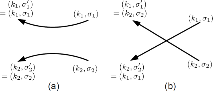
Figure 23: Feynman diagrams for calculating the (a) direct and (b) the exchange contribution the the average SQM.

The momenta in the final states are the same as for the initial states, $k_{i}=k_{i^{\prime}}$, since the SQM operator does not act on the orbital part of the wave function (cf. Eq. (166)). Two different scattering processes are permitted: the first one is a direct scattering, for which the electron in initial state $i$ ends up in state $i^{\prime}$, restricting the spin indices to $\sigma_{i}=\sigma_{i}^{\prime}$ (while already $k_{i}=k_{i^{\prime}}$). These direct scattering contributions, multiplied with their tensor-valued amplitudes $\mathbf{s}_{\sigma_{1}\sigma_{2}}\odot\mathbf{s}_{\sigma_{2}\sigma_{1}}$ in (150) add up to the direct SQM. This contribution to the spin anisotropy is thus generated by two electrons (labelled by their states $1$ and 2) as if they were distinguishable, i.e., by treating the two-particle scattering classically.

The second type of scattering process, in which the particles are exchanged, accounts for the fact that electrons are indistinguishable. This is only possible if the momenta are the same, $k_{1}=k_{2}$, and furthermore, the spins are exchanged, $\sigma_{1}^{\prime}=\sigma_{2}$ and $\sigma_{2}^{\prime}=\sigma_{1}$. This exchange contribution to the average SQM entirely cancels the direct contribution for equal $k_{1}=k_{2}$, correcting for the treatment of electrons as distinguishable particles. In other words, the exchange SQM accounts for Pauli “holes” in the triplet spin-spin correlation tensor. The Pauli principle thus counters the direct classical contribution to the spin anisotropy.

Indistinguishability becomes important if we consider pairs of electrons from the same $k$-mode. Due to Pauli’s principle, their wave function must have a symmetric orbital part and an antisymmetric spin part, that is, they form a spin singlet with zero SQM, i. e., triplet correlations are forbidden. This is analogous to the direct and exchange contributions to the average Coulomb interaction with respect to Slater determinants (e.g., in Hartree-Fock theory). In that case, nearby electrons with parallel spins repel each other due to the exchange potential. We mention that as expected from this analogy, thermal fluctuations suppress the effect of the Pauli principle on SQM as well, c.f. Eq. (182) below.

A.2 Spin-Trace Technique

We now reformulate the above calculation in a way that will be used in the transport calculations (cf. Sec. E.4): the result (161) then assumes the coordinate-free form presented in Sec. III.2.3.

$$\langle\bm{\mathcal{Q}}^{rr}\rangle_{\mathrm{ex}} = \sum_{k\sigma\sigma^{\prime}\tau\tau^{\prime}}\left(\mathbf{s}^{r}_{\sigma\sigma^{\prime}}\odot\mathbf{s}^{r}_{\tau\tau^{\prime}}\right)\delta_{\sigma\tau^{\prime}}\delta_{\sigma^{\prime}\tau}$$ (152)

$$\times f_{+}^{r}(\varepsilon^{r}_{k\sigma})f^{r}_{-}(\varepsilon^{r}_{k\sigma^{\prime}}).$$

Here we reintroduced the electrode index. To recast this into covariant expression, we first introduce the two-particle density of states (16),

$$\nu^{r}_{\sigma\sigma^{\prime}}(\omega,\omega^{\prime}) = \sum_{n,k}\delta(\omega-\varepsilon^{r}_{k\sigma})\delta(\omega^{\prime}-\varepsilon^{r}_{k\sigma^{\prime}}),$$ (153)

and rewrite Eq. (152) in terms of frequency integrals

$$\langle\bm{\mathcal{Q}}^{rr}\rangle_{\mathrm{ex}}=\sum_{k\sigma\sigma^{\prime}\tau\tau^{\prime}}\int d\omega d\omega^{\prime}\left(\mathbf{s}^{r}_{\sigma\sigma^{\prime}}\odot\mathbf{s}^{r^{\prime}}_{\tau\tau^{\prime}}\right)$$

$$\delta_{\sigma\tau^{\prime}}\delta_{\sigma^{\prime}\tau}\nu_{\sigma\sigma^{\prime}}(\omega,\omega^{\prime})f_{+}^{r}(\omega)f^{r}_{-}(\omega^{\prime}).$$ (154)

The 2DOS $\nu^{r}_{\sigma\sigma^{\prime}}(\omega)$ can be expressed as a matrix element in spin space by

$$\nu^{r}_{\sigma\sigma^{\prime}}(\omega,\omega^{\prime})\delta_{\sigma\tau^{\prime}}\delta_{\sigma^{\prime}\tau}$$ (155)

$$= 2\sum_{\mu_{1},\mu_{2}}\text{}^{r}\langle\tau^{\prime}|\check{r}_{\mu_{1}}|\sigma\rangle^{r}\bm{\mathcal{A}}^{r}_{\mu_{1}\mu_{2}}(\omega,\omega^{\prime})^{r}\langle\sigma^{\prime}|\check{r}_{\mu_{2}}|\tau\rangle^{r}.\hskip 10.00002pt$$

Here we used the four component operator $\mathbf{\check{r}}$ with $\check{r}_{0}=\mathbbm{1}\text{/}\sqrt{2}$ and $\check{r}_{i}=\sqrt{2}s_{i}\text{}$ for $i=x,y,z$. The four dimensional matrix $\bm{\mathcal{A}}^{r}_{\mu_{1}\mu_{2}}$ incorporates all relevant 2DOS information. It decomposes into a scalar, two vectors and a tensor in coordinate space:

$$\bm{\mathcal{A}}_{00}^{r} = \frac{1}{4}\overset{}{\sum_{\sigma\sigma^{\prime}}}\nu^{r}_{\sigma\sigma^{\prime}}(\omega,\omega^{\prime}),$$ (156)

$$\bm{\mathcal{A}}_{i0}^{r} = \frac{1}{4}\overset{}{\sum_{\sigma\sigma^{\prime}}}\sigma\nu^{r}_{\sigma\sigma^{\prime}}(\omega,\omega^{\prime})\hat{J}^{r}_{i},$$ (157)

$$\bm{\mathcal{A}}_{0j}^{r} = \frac{1}{4}\overset{}{\sum_{\sigma\sigma^{\prime}}}\sigma^{\prime}\nu^{r}_{\sigma\sigma^{\prime}}(\omega,\omega^{\prime})\hat{J}^{r}_{j},$$ (158)

$$\bm{\mathcal{A}}_{ij}^{r} = \frac{1}{4}\overset{}{\sum_{\sigma\sigma^{\prime}}}\sigma\sigma^{\prime}\nu^{r}_{\sigma\sigma^{\prime}}(\omega,\omega^{\prime})\hat{J}^{r}_{i}\hat{J}^{r}_{j}.$$ (159)

Inserting Eq. (155) into Eq. (154) and recasting the sum over the spin indices as a trace in spin space yields

$$\langle\bm{\mathcal{Q}}^{rr}\rangle_{\mathrm{ex}} = \int d\omega d\omega^{\prime}f^{r}_{+}(\omega)f^{r}_{-}(\omega^{\prime})$$ (161)

$$2\sum_{\mu_{1}\mu_{2}}\bm{\mathcal{A}}^{r}_{\mu_{1}\mu_{2}}(\omega,\omega^{\prime})\text{Tr}\left[\check{r}_{\mu_{1}}\mathbf{s}\odot\check{r}_{\mu_{2}}\mathbf{s}\right]$$

$$= \int d\omega d\omega^{\prime}\overset{}{\tfrac{1}{4}\sum_{\sigma\sigma^{\prime}}}\sigma\sigma^{\prime}\nu^{r}_{\sigma\sigma^{\prime}}(\omega,\omega^{\prime})$$

$$\times f^{r}_{+}(\omega)f^{r}_{-}(\omega^{\prime})\widehat{\mathbf{J}}^{r}\odot\widehat{\mathbf{J}}^{r}.$$

This recovers the results (66)-(69) obtained in the main text from Eq. (150). The explicit calculation in the last step is now reduced to using spin-1/2 operator algebra $s_{i}s_{j}=\tfrac{1}{4}\delta_{ij}\mathbbm{1}+\tfrac{1}{2}\sum_{k}i\varepsilon_{ijk}s_{k}$ and $\mathbf{s}\odot\mathbf{s}=0$, i.e., without using matrix elements. These steps are analogous to the evaluation of the diagrammatic expressions for the SQM current in App. D.

A.3 SQM and Triplet Spin Correlations

Finally, we express the SQM tensor operator $\bm{\mathcal{Q}}$ in the second-quantized form. This allows one to perform vector-coupling of the pairs of involved spin, thereby making explicit that only triplet correlations are “measured” by $\langle\bm{\mathcal{Q}}\rangle$, something that did not become clear in the above calculations. This is merely important for the physical understanding, but seems to bring no advantage for calculations. The many-body quadrupole operator is a sum over quadrupole operators of pairs of particles, the latter labeled by $a,b=1,2,3,\ldots$

$$\bm{\mathcal{Q}} = \sum_{a<b}\bm{\mathcal{Q}}^{ab}$$ (162)

with  Cartesian components $i,j=x,y,z$:

$$Q^{ab}_{ij} = 2\left(\tfrac{1}{2}(s^{a}_{i}s^{b}_{j}+s^{a}_{j}s^{b}_{i})-\tfrac{1}{3}\mathcal{\delta}_{ij}\sum_{k}s^{a}_{k}s_{k}^{b}\right).$$ (163)

Here we inserted the total spin operator $\mathbf{S}=\sum_{a}\mathbf{s}^{a}$ into Eq. (1) and used the result $\bm{\mathcal{Q}}^{aa}=0$ (‘a ‘single electron has no anisotropy”, cf. Sec. II.1). The SQM from pair $\langle ab\rangle$ can also be expressed by introducing coupling the two spins to $\mathbf{S}^{ab}=\mathbf{s}^{a}+\mathbf{s}^{b}$,

$$Q^{ab}_{ij} = \tfrac{1}{2}(S^{ab}_{i}S^{ab}_{j}+S^{ab}_{j}S^{ab}_{i})-\tfrac{1}{3}\delta_{ij}\left(\mathbf{S}^{ab}\right)^{2},$$ (164)

using $s^{a}_{i}s_{j}^{a}=\tfrac{1}{4}\delta_{ij}+i\tfrac{1}{2}\sum_{k}\varepsilon_{ijk}s_{k}^{a}$. Note the factor 2 in Eq. (163). The general second quantization prescription immediately gives

$$\bm{\mathcal{Q}} = \sum_{\{k_{i}\sigma_{i}\}}\tfrac{1}{2}\langle k_{2}^{\prime}\sigma_{2}^{\prime}k_{1}^{\prime}\sigma_{1}^{\prime}|\mathcal{\bm{\mathcal{Q}}}^{12}|k_{2}\sigma_{2}k_{1}\sigma_{1}\rangle$$ (165)

$$c^{{\dagger}}_{k_{1}^{\prime}\sigma_{1}^{\prime}}c^{{\dagger}}_{k_{2}^{\prime}\sigma_{2}^{\prime}}c_{k_{2}\sigma_{2}}c_{k_{1}\sigma_{1}}.$$

We now make explicit use the particular property of the matrix elements of the pair SQM $\bm{\mathcal{Q}}^{12}$. First, we note that $\bm{\mathcal{Q}}^{12}$ acts only on the spin of the electrons,

$$\langle k_{2}^{\prime}\sigma_{2}^{\prime}k_{1}^{\prime}\sigma_{1}^{\prime}|\mathcal{\bm{\mathcal{Q}}}^{12}|k_{2}\sigma_{2}k_{1}\sigma_{1}\rangle$$ (166)

$$= \delta_{k_{2}^{\prime}k_{2}}\delta_{k_{1}^{\prime}k_{1}}\langle\sigma_{2}^{\prime}\sigma_{1}^{\prime}|\mathcal{\bm{\mathcal{Q}}}^{12}|\sigma_{2}\sigma_{1}\rangle.$$

If we inserted this into Eq. (165) we would recover Eq. (146). Instead of this, we now introduce a singlet-triplet basis for each pair of  considered spins $\sigma_{1}$ and $\sigma_{2}$ above:

$$|S\rangle = \tfrac{1}{\sqrt{2}}\sum_{\sigma}\sigma|\sigma\bar{\sigma}\rangle,$$ (167)

$$|T0\rangle = \tfrac{1}{\sqrt{2}}\sum_{\sigma}|\sigma\bar{\sigma}\rangle,$$ (168)

$$|Tm\rangle = |mm\rangle,\text{ \ \ \ \ }m=\pm$$ (169)

where $\bar{\sigma}=-\sigma$. The crucial point is that $\bm{\mathcal{Q}}^{12}$ only has matrix elements in the triplet sector. This follows from the fact that $\bm{\mathcal{Q}}^{12}$ is symmetric under exchange of the spins, i.e., $\left[P,\bm{\mathcal{Q}}^{12}\right]=0$ where $P$ is the exchange operator. Therefore $\bm{\mathcal{Q}}^{12}$ is block-diagonal with respect to the eigen spaces of $P$, which are here the singlet and triplet states satisfying $P|S\rangle=-|S\rangle$ and $P|Tm\rangle=+|Tm\rangle$. Thus, $\langle S|\bm{\mathcal{Q}}^{12}|Tm\rangle=\langle Tm|\bm{\mathcal{Q}}^{12}|S\rangle=0$. Moreover, the diagonal singlet block is zero, $\langle S|\bm{\mathcal{Q}}^{12}|S\rangle=0$ by Eq. (164) with $a=1,b=2$ and $\mathbf{S}^{12}|S\rangle=0$, completing the proof. As a result

$$\langle\sigma_{2}^{\prime}\sigma_{1}^{\prime}|\mathcal{\bm{\mathcal{Q}}}^{12}|\sigma_{2}\sigma_{1}\rangle=$$

$$\sum_{mm^{\prime}}\langle\sigma_{2}^{\prime}\sigma_{1}^{\prime}|Tm\rangle\langle Tm|\bm{\mathcal{Q}}\mathcal{}^{12}|Tm^{\prime}\rangle\langle Tm^{\prime}|\sigma_{2}\sigma_{1}\rangle.\hskip 10.00002pt$$ (170)

Inserting Eq. (170) into Eq. (165), we obtain the central result of the appendix,

$$\bm{\mathcal{Q}} = \sum_{mm^{\prime}}\tfrac{1}{2}\langle Tm^{\prime}|\mathcal{\bm{\mathcal{Q}}}^{12}|Tm\rangle\sum_{\{k_{i}\}}E^{m^{\prime}{\dagger}}_{k_{2}k_{1}}E^{m}_{k_{2}k_{1}},$$ (171)

with two-particle operators that explicitly generate only triplet pairs:

$$E^{m}_{k_{2}k_{1}} = \sum_{\sigma_{2}\sigma_{1}}\langle Tm|\sigma_{2}\sigma_{1}\rangle c_{k_{2}\sigma_{2}}c_{k_{1}\sigma_{1}}$$ (172)

$$= \left\{\begin{array}[]{ll}c_{k_{2}m}c_{k_{1}m}&m=\pm 1\\ \frac{1}{\sqrt{2}}\sum_{\sigma}c_{k_{2}\sigma}c_{k_{1}\bar{\sigma}}&m=0\end{array}\right..$$ (175)

Considered as an interaction, $\bm{\mathcal{Q}}$ thus only scatters triplet correlated pairs of electrons. Due to the restrictions on the spins in these operators $E^{m}_{k_{2}k_{1}}$, the averages are

$$\langle E^{m^{\prime}{\dagger}}_{k_{2}k_{1}}E^{m}_{k_{2}k_{1}}\rangle=\delta_{mm^{\prime}}\times$$

$$\left\{\begin{array}[]{ll}f(\varepsilon_{k_{2}m})f(\varepsilon_{k_{1}m})(1-\delta_{k_{2}k_{1}}),&m=\pm 1\\ \tfrac{1}{2}\sum_{\sigma}f(\varepsilon_{k_{2}\sigma})f(\varepsilon_{k_{1}\bar{\sigma}})(1-\delta_{k_{2}k_{1}}),&m=0\end{array}\right.$$ (178)

with the tensor-valued matrix elements $\langle T+|\mathcal{\bm{\mathcal{Q}}}^{12}|T+\rangle=\langle T-|\mathcal{\bm{\mathcal{Q}}}^{12}|T-\rangle=-\langle T0|\mathcal{\bm{\mathcal{Q}}}^{12}|T0\rangle/2=\tfrac{1}{2}\mathbf{e}_{z}\odot\mathbf{e}_{z}$ given by Eqs. (2)-(3) in the main text. These relations follow from the fact that $\bm{\mathcal{Q}}^{12}$ is traceless in the Hilbert space, $\sum_{m=0,\pm 1}\langle Tm|\mathcal{\bm{\mathcal{Q}}}^{12}|Tm\rangle=0$ and that the $m=\pm$ states have the identical spin-anisotropy. We recover Eq. (150):

$$\langle\bm{\mathcal{Q}}\rangle=\tfrac{1}{4}\mathbf{e}_{z}\odot\mathbf{e}_{z}\sum_{k_{2}k_{1}}(1-\delta_{k_{2}k_{1}})$$

$$\times\left(\sum_{m=\pm}f_{+}(\varepsilon_{k_{2}m})f_{+}(\varepsilon_{k_{1}m})\right.$$

$$-\left.\sum_{\sigma=\pm}f_{+}(\varepsilon_{k_{2}\sigma})f_{+}(\varepsilon_{k_{1}\bar{\sigma}})\right)$$ (179)

This derivation, however, shows explicitly that the $m=\pm 1$ terms contribute the same, uniaxial anisotropy tensor $\langle T\pm|\mathcal{\bm{\mathcal{Q}}}^{12}|T\pm\rangle$, whereas the $m=0$ term contributes an easy-plane anisotropy tensor $\langle T0|\mathcal{\bm{\mathcal{Q}}}^{12}|T0\rangle=-2\langle T+|\mathcal{\bm{\mathcal{Q}}}^{12}|T+\rangle$. Moreover, the Pauli-exclusion hole factor $1-\delta_{k_{2}k_{1}}$ is immediately explicit. Thus, $\langle\bm{\mathcal{Q}}\rangle$ can be calculated by first accounting for triplet correlations between spins of pairs of electrons in all possible orbitals, including the same orbital,

$$\langle\bm{\mathcal{Q}}\rangle_{\mathrm{dir}} = \tfrac{1}{4}\sum_{k_{2}k_{1}\sigma_{2}\sigma_{1}}\sigma_{2}f(\varepsilon_{k_{2}\sigma_{2}})\sigma_{1}f(\varepsilon_{k_{1}\sigma_{1}})\mathbf{e}_{z}\odot\mathbf{e}_{z}$$ (180)

$$= \langle\mathbf{S}\rangle\odot\langle\mathbf{S}\rangle,$$

giving Eq. (59), and then subsequently cancelling the latter violation of the Pauli principle by the exchange term,

$$\langle\bm{\mathcal{Q}}\rangle_{\mathrm{ex}} = -q_{\mathrm{ex}}\mathbf{e}_{z}\odot\mathbf{e}_{z}$$ (181)

with the positive exchange magnitude

$$q_{\mathrm{ex}} = \tfrac{1}{4}\sum_{k}(f_{+}(\varepsilon_{k\uparrow})-f_{+}(\varepsilon_{k\downarrow}))^{2}.$$ (182)

We obtain Eq. (64) from the main text. Finally, we show that the two-particle DOS $\nu_{\sigma\sigma^{\prime}}$ can be decomposed explicitly into triplet DOS components: converting the sums in Eq. (182) to integrals we obtain

$$q_{\mathrm{ex}} = \int d\omega d\omega^{\prime}f_{+}(\omega)f_{+}(\omega^{\prime})\sum_{\sigma\sigma^{\prime}}\sigma\sigma^{\prime}\nu^{r}_{\sigma\sigma^{\prime}}(\omega,\omega^{\prime}).$$ (183)

The only relevant combination of the 2DOS in the above expression can be recast as

$$\sum_{\sigma\sigma^{\prime}}\sigma\sigma^{\prime}\nu^{r}_{\sigma\sigma^{\prime}} = \nu^{r}_{T+}+\nu_{T-}^{r}-\sqrt{2}\nu^{r}_{T0}$$ (184)

with the triplet exchange 2DOS function ($m=\pm$)

$$\nu^{r}_{Tm}(\omega,\omega^{\prime}) := \nu^{r}_{mm}(\omega,\omega^{\prime}),$$ (185)

$$\nu^{r}_{T0}(\omega,\omega^{\prime}) := \frac{1}{\sqrt{2}}\sum_{\sigma}\nu^{r}_{\sigma\bar{\sigma}}(\omega,\omega^{\prime}).$$ (186)

This gives a precise decomposition into triplet spin correlations that contribute to $\langle\bm{\mathcal{Q}}^{rr}\rangle_{\mathrm{ex}}$.

A.4 Spin-anisotropy Function

Finally, we further substantiate the physical interpretation of the anisotropy function, which plays a key role in the main text. The basic idea of “quadrupolarization” of two triplet-correlated electrons is simply to “count” whether the spins are parallel ($\uparrow\uparrow$ or $\downarrow\downarrow$, counted as $+$), or antiparallel ($\uparrow\downarrow$ or $\downarrow\uparrow$, counted as $-$). In both cases their individual orientations, i.e., their dipolarization $\uparrow$ or $\downarrow$, is ignored. Eq. (183) precisely expresses this notion for the exchange SQM. It is instructive to start from the $k$-sum representation (182) and to write it as

$$q_{\mathrm{ex}} = \sum_{k\sigma}f_{+}(\varepsilon_{k\sigma})a_{k\sigma}.$$ (187)

Here, given that an electron with spin $\sigma$ occupies orbital $k$, we “count” by

$$a_{k\sigma} = \sum_{\sigma^{\prime}}\tfrac{\sigma\sigma^{\prime}}{4}f(\varepsilon_{k\sigma^{\prime}})$$ (188)

the average quadrupolarization contribution from electrons in that same orbital $k$: parallel spin $\sigma^{\prime}=\sigma$ gives $+f_{+}(\varepsilon_{k\sigma})$, antiparallel $\sigma^{\prime}=\bar{\sigma}$ gives $-f(\varepsilon_{k\bar{\sigma}})$. Converting the sum to an integral, we obtain Eq. (66) of the main text:

$$q_{\mathrm{ex}} = \int\mathrm{d}\omega f_{+}(\omega)\bar{\nu}(\omega)a(\omega).$$ (189)

The anisotropy function $a(\omega)=\sum_{\sigma}a_{\sigma}(\omega)$ has two contributions:

$$\bar{\nu}(\omega)a_{\sigma}(\omega) := \sum_{k}a_{k\sigma}\delta(\omega-\varepsilon_{k\sigma}).$$ (190)

The quantity $\bar{\nu}(\omega)a_{\sigma}(\omega)$ is the exchange quadrupolarization of a spin $\sigma$ electron at energy $\omega$. One should note that the function $a_{k\sigma}$, defined by Eq. (188), does not only depend on the energy $\varepsilon_{k\sigma}$, but also on the energy $\varepsilon_{k\bar{\sigma}}$. Since $\varepsilon_{k\bar{\sigma}}$ is not necessarily an implicit function of $\varepsilon_{k\sigma}$ for arbitrary band structures, one can in general reformulate Eq. (190) only in terms of the 2DOS (16):

$$\bar{\nu}(\omega)a_{\sigma}(\omega) = \int\mathrm{d}\omega^{\prime}f_{+}(\omega^{\prime})\sum_{\sigma^{\prime}}\tfrac{\sigma\sigma^{\prime}}{4}\nu_{\sigma\sigma^{\prime}}(\omega,\omega^{\prime}),$$ (191)

resulting in Eq. (69) of the main text.

However, for the Stoner model, which we discuss from hereon, the simple relation $\varepsilon_{k\bar{\sigma}}=\varepsilon_{k\sigma}-\sigma J\text{/}2$ can be exploited to express $a_{k\sigma}$ as a function of $\varepsilon_{k\sigma}$ only. We therefore obtain the simpler result

$$\bar{\nu}(\omega)a_{\sigma}(\omega) = \nu_{\sigma}(\omega)(f_{+}(\omega)-f_{+}(\omega+\sigma J)),$$ (192)

which only depends on the 1DOS $\nu_{\sigma}$. This unfortunately hides the underlying two-particle nature of the exchange SQM, but aids the interpretation of the total spin-anisotropy function: Eq. (192) shows that the contribution $a_{\uparrow}(\omega)$ from up-spins is positive and comes from the range of energies $\mu-J<\omega<\mu$, whereas the contribution $a_{\downarrow}(\omega)$ from down-spins is negative and comes from energies  $\mu<\omega<\mu+J$ (both up to thermal smearing). Adding both contributions yields for the full spin-anisotropy function after some manipulations

$$a(\omega) = \tfrac{1}{4}[2f_{+}(\omega)-f_{+}(\omega+J)-f_{+}(\omega-J)]$$ (193)

$$+\tfrac{1}{4}n(\omega)[f_{+}(\omega+J)-f_{+}(\omega-J)].$$

Here it should be noted that $n(\omega)$ is not independent of $J$ but is a function of it through Eq. (13),  (15) and (18). The combinations of Fermi-functions are non-zero only for energies $|\omega-J|\lesssim T$.

It was pointed out in Sec. V.3 for a purely thermally biased tunnel junction that the finite SQM current that remains whenever the spin current vanishes arises entirely from the exchange SQM, i.e., from the antisymmetric part of the spin-anisotropy function $a(\omega)$ relative to $\mu$. Generally, when assuming a weakly energy dependent average DOS $\bar{\nu}(\omega)$ in the range $|\omega-J|\lesssim T$, the first term Eq. (193) always gives rise to such a term. The second term, in which the spin-polarization $n(\omega)$ is multiplied by a symmetric function relative to $\mu$, can only cancel this function if $n(\omega)$ is strongly antisymmetric (i.e., $n(\omega)=\pm 1$ for $\omega\gtrless 0$, up to thermal smearing). If we further specialize to the approximation of a flat band symmetric about $\mu$ (cf. Sec. II.4), this second term is exactly zero because the spin polarization vanishes in the window $[\omega-J,\omega+J]$ up to thermal smearing. Only the first line of Eq. (193) remains and gives a thermally induced pure SQM current as discussed in Sec. V.3: substituting $x=(\omega-\mu)\text{/}T$, Eq. (189) can be rewritten as

$$q_{\mathrm{ex}} = \frac{\bar{\nu}T}{4}\int\mathrm{d}xf(x)[2f(x)-f(x-j)-f(x+j)],\quad$$ (194)

where $f(x)=[e^{x}+1]^{-1}$ and $j=J\text{/}T$. As $a(\omega)$ is nonzero in an energy window $2J$ centered at $\mu$, which is far away from the band edges, we can replace the 1DOS by its constant value $\bar{\nu}$ and extend the limits integration to $\pm\infty$. Using the identity $f(x)=1-f(-x)$ and the result

$$\int dxf(x)f(-(x-y)) = \left\{\begin{array}[]{ll}1&y=0\\ yb(y)&\text{else}\end{array},\right.$$ (197)

where $b(x)=[e^{x}-1]^{-1}$ is the Bose function, and taking the limit $y\rightarrow 0$ we obtain Eq. (72) of the main text:

$$q_{\mathrm{ex}} = \frac{\bar{\nu}}{4}[-2+jb(j)+(-j)b(-j)]$$ (198)

$$= \frac{\bar{\nu}}{2}\left[\frac{j}{2}\coth\left(\frac{j}{2}\right)-1\right].$$ (199)

Appendix B Symmetric and Traceless Tensors

In this appendix, we collect some relevant results on symmetric, traceless tensors. We first show how a particular type of such tensors, constructed from two real vectors $\mathbf{a}$ and $\mathbf{b}$,

$$\begin{array}[]{lllll}\mathcal{A}&=&\mathbf{a}\odot\mathbf{b}&=&\frac{1}{2}\left(\mathbf{a}\mathbf{b}+\mathbf{b}\mathbf{a}\right)-\frac{1}{3}\left(\mathbf{a}\cdot\mathbf{b}\right)\mathcal{I},\end{array}$$ (201)

can be diagonalized using dyadic calculus Lindell (1992), i. e., without introducing a coordinate system. The tensor $\mathcal{A}$ can be expressed in terms of its principal values $\lambda_{\mu}$ and normalized vectors $\hat{\mathbf{v}}_{\mu}$ that define the principal axes as

$$\mathcal{A} = \overset{}{\sum_{\mu=0,\pm}}\lambda_{\mu}\hat{\mathbf{v}}_{\mu}\hat{\mathbf{v}}_{\mu}^{T}.$$ (202)

The results (130)-(139) of the main text can then be obtained from Eq. (122) by setting $\mathbf{a}=\hat{\mathbf{J}}^{L}$ and $\mathbf{b}=E^{L}\hat{\mathbf{J}}^{L}+A^{L}\hat{\mathbf{J}}^{R}+T^{L}\left(\hat{\mathbf{J}}^{L}\times\hat{\mathbf{J}}^{R}\right)$. To diagonalize (201), we have to distinguish two cases:

Case (i) $\mathbf{\mathbf{a}\nparallel\mathbf{b}}$: eigenvalues

$$\lambda_{\mu} = -\tfrac{1}{3}\left(\mathbf{a}\cdot\mathbf{b}\right)+\tfrac{1}{2}\delta_{\mu,\pm}\left[\left(\mathbf{a}\cdot\mathbf{b}\right)+\mu ab\right],$$ (203)

where $\mu=0,\pm$ and normalized eigenvectors

$$\hat{\mathbf{v}}_{0} = \frac{1}{\left|\mathbf{a}\times\mathbf{b}\right|}\left(\mathbf{a}\times\mathbf{b}\right),$$ (204)

$$\hat{\mathbf{v}}_{\pm} = \frac{1}{2ab\left(ab\pm\left(\mathbf{a}\cdot\mathbf{b}\right)\right)}\left[a\mathbf{b}\pm b\mathbf{a}\right]$$ (205)

with $a=\left|\mathbf{a}\right|,b=\left|\mathbf{b}\right|$.

Case (ii) $\mathbf{a}\parallel\mathbf{b}$, i. e., $\mathbf{b}=\alpha\mathbf{a}$: eigenvalues for $\mu=0,\pm$

$$\lambda_{\mu} = \left(\delta_{\mu,+}-\tfrac{1}{3}\right)\alpha a^{2},$$ (206)

and $\hat{\mathbf{v}}_{+}=\mathbf{a}\text{/}a$ and $\hat{\mathbf{v}}_{0}$,  $\hat{\mathbf{v}}_{-}$  are any two orthonormal vectors that span the plane perpendicular to $\hat{\mathbf{v}}_{+}$.

To prove case (i), we first note that one principal axis is obviously $\mathbf{v}_{0}=\mathbf{a}\times\mathbf{b}\neq 0$:

$$\mathcal{A}\cdot\mathbf{v}_{0} = \left[\tfrac{1}{2}\left(\mathbf{a}\mathbf{b}+\mathbf{b}\mathbf{a}\right)-\tfrac{1}{3}\left(\mathbf{a}\cdot\mathbf{b}\right)\mathcal{I}\right]\cdot\left(\mathbf{a}\times\mathbf{b}\right)$$ (207)

$$= -\tfrac{1}{3}\left(\mathbf{a}\cdot\mathbf{v}\right)\mathbf{v}_{0}=\lambda_{0}\mathbf{v}_{0}.$$ (208)

In order to derive the the remaining principal values, we need to set up the characteristic equation:

$$0 = \det\left(\mathcal{\bm{\mathcal{A}}}-\lambda\bm{\mathcal{I}}\right)$$ (209)

$$= \det\left(\mathcal{\bm{\mathcal{A}}}\right)-\lambda\mathrm{spm}\left(\bm{\mathcal{A}}\right)+\lambda^{2}\mathrm{tr}\left(\mathcal{\bm{\mathcal{A}}}\right)-\lambda^{3},$$ (210)

where the coefficients are given by the trace, the sum of principal minors and the determinant of $\mathcal{\bm{\mathcal{A}}}$, respectively:

$$\mathrm{tr}\left(\bm{\mathcal{A}}\right) = \sum_{i}\mathcal{\bm{\mathcal{A}}}_{ii},$$ (211)

$$\mathrm{spm}\left(\bm{\mathcal{A}}\right) = \tfrac{1}{2}\mathrm{tr}\left(\mathcal{\bm{\mathcal{A}}}^{\times}_{\times}\mathcal{\bm{\mathcal{A}}}\right),$$ (212)

$$\det\left(\bm{\mathcal{A}}\right) = \tfrac{1}{6}\left(\mathcal{\bm{\mathcal{A}}}^{\times}_{\times}\bm{\mathcal{\mathcal{A}}}\right):\bm{\mathcal{\mathcal{A}}}.$$ (213)

Here we used the shorthand notations  $\begin{array}[]{lll}\left(\mathcal{\bm{\mathcal{A}}}^{\times}_{\times}\mathcal{\bm{\mathcal{A}}}\right)_{i_{1}i_{2}}&=&\varepsilon_{i_{1}j_{1}k_{1}}\mathcal{\bm{\mathcal{A}}}_{j_{1}j_{2}}\mathcal{\bm{\mathcal{A}}}_{k_{1}k_{2}}\varepsilon_{j_{2}k_{2}i_{2}}\end{array}$ and  $\mathcal{\bm{\mathcal{B}}}:\mathcal{\bm{\mathcal{A}}}=\sum_{i,j}\bm{\mathcal{\mathcal{B}}}_{ij}\mathcal{\bm{\mathcal{A}}}_{ij}$. Eqs. (211)-(213) are the (only) three rotational invariants, i. e. they are invariant under transformations $\mathcal{\bm{\mathcal{A}}}\rightarrow\mathcal{\bm{\mathcal{R}}}\cdot\mathcal{\bm{\mathcal{A}}}\cdot\mathcal{\bm{\mathcal{R}}}^{T}$ where $\mathcal{\bm{\mathcal{R}}}$ is a rotation matrix: $\mathcal{\bm{\mathcal{R}}}\cdot\bm{\mathcal{\mathcal{R}}}^{T}=\bm{\mathcal{\mathcal{R}}}^{T}\cdot\mathcal{\bm{\mathcal{R}}}=\mathcal{\bm{\mathcal{I}}}$. Inserting Eq. (201) we obtain

$$\mathrm{tr}\left(\mathcal{\bm{\mathcal{A}}}\right) = \left(\mathbf{a}\cdot\mathbf{b}\right),$$ (214)

$$\mathrm{spm}\left(\mathcal{\bm{\mathcal{A}}}\right) = -\tfrac{1}{3}\left(\mathbf{a}\cdot\mathbf{b}\right)^{2}-\tfrac{1}{4}\left(\mathbf{a}\times\mathbf{b}\right)^{2},$$ (215)

$$\det\left(\mathcal{\bm{\mathcal{A}}}\right) = \tfrac{2}{27}\left(\mathbf{a}\cdot\mathbf{b}\right)^{3}+\tfrac{1}{12}\left(\mathbf{a}\cdot\mathbf{b}\right)\left(\mathbf{a}\times\mathbf{b}\right)^{2}.$$ (216)

Inserting these into Eq. (210), one finds that $\lambda_{0}$, given by (203) with $\mu=0$, is indeed a principal value of $\mathcal{\bm{\mathcal{A}}}$. By polynomial division we obtain a quadratic equation for the remaining principal values $\lambda_{\pm}$, which is solved by Eq. (203) with $\mu=\pm$. The general solution of $\begin{array}[]{l}\left(\bm{\mathcal{\mathcal{A}}}-\lambda_{\pm}\mathcal{\bm{\mathcal{I}}}\right)\cdot\mathbf{v}_{\pm}=0\end{array}$is given by Lindell (1992):

$$\mathbf{v}_{\pm} = \mathbf{c}\cdot\left[\left(\mathcal{\bm{\mathcal{A}}}-\lambda_{\pm}\mathcal{\bm{\mathcal{I}}}\right)^{\times}_{\times}\left(\mathcal{\bm{\mathcal{A}}}-\lambda_{\pm}\mathcal{\bm{\mathcal{I}}}\right)\right]$$ (218)

$$= -\tfrac{1}{2}\mathbf{c}\cdot\left[{\color[rgb]{1,1,1}]}\left.\left(\mathbf{a}\times\mathbf{b}\right)\right.\left(\mathbf{a}\times\mathbf{b}\right)\right.$$

$$\left.+\left(2q_{\pm}\left(\mathbf{a}\cdot\mathbf{b}\right)-q_{\pm}^{2}\right)\bm{\mathcal{\mathcal{I}}}-q_{\pm}\left(\mathbf{a}\mathbf{b}+\mathbf{b}\mathbf{a}\right)\right].$$

where  $q_{\pm}=\left(\mathbf{a}\cdot\mathbf{b}\right)\pm\left|\mathbf{a}\right|\left|\mathbf{b}\right|$. Here $\mathbf{c}$ is a vector such that $\mathbf{v}_{\pm}\neq 0$ and either $\mathbf{c}=\mathbf{a}$ or $\mathbf{c}=\mathbf{b}$ fulfills this condition, yielding the result (205) after normalization.

For case (ii) we have $\bm{\mathcal{\mathcal{A}}}=\mathbf{a}\odot\alpha\mathbf{a}=\alpha\left(\mathbf{a}\mathbf{a}-a^{2}\mathcal{\bm{\mathcal{I}}}/3\right)$. Since $\mathbf{a}\times\mathbf{b}=0$, the above results cannot be applied. The vector $\mathbf{a}$ obviously defines a principal axes since $\mathcal{\bm{\mathcal{A}}}\cdot\mathbf{a}=+\tfrac{2}{3}\alpha a^{2}\mathbf{a}$, and for any vector $\mathbf{a}_{\perp}$ in the plane perpendicular to $\mathbf{a}$ we have $\bm{\mathcal{\mathcal{A}}}\cdot\mathbf{a}_{\perp}=-\tfrac{1}{3}\alpha a^{2}$. This confirms the principal values (206), completing the proof.

Appendix C Rotation of the SQM by SQM Currents

In this appendix we show that a SQM tensor $\bm{\mathcal{Q}}$ is rotated if it does not commute with the SQM current tensor $\bm{\mathcal{I}}_{\bm{\mathcal{Q}}}$ as pointed out in V.2.3. More formally,  $\left[\bm{\mathcal{Q}},\bm{\mathcal{I}}_{\bm{\mathcal{Q}}}\right]_{-}=0$ implies the both tensors have collinear principal axes. We outline the analogous situation for the spin vector: it is geometrically clear that the spin $\mathbf{S}$ does not rotate, that is, $\mathbf{S}=S(t)\mathbf{e}_{3}$ in some time-independent basis if and only if the spin current vector $\mathbf{I}_{\mathbf{S}}=\dot{\mathbf{S}}$ is collinear to $\mathbf{S}$ at all times.

We now outline a proof of this statement, which can be extended to the SQM. Assume $\mathbf{S}$ does not rotate, then $\mathbf{S}=S(t)\mathbf{e}_{3}$  in some time independent basis $\mathbf{e}_{i}$ and. Then $\dot{\mathbf{S}}=\dot{S}(t)\mathbf{e}_{3}=\mathbf{I}_{\mathbf{S}}$. Thus, $\mathbf{I}_{\mathbf{S}}\cdot\mathbf{S}=\pm\left|\mathbf{S}\right|\left|\mathbf{I}_{\mathbf{S}}\right|\mathbf{e}_{3}\cdot\mathbf{e}_{3}=\pm\left|\mathbf{S}\right|\left|\mathbf{I}_{\mathbf{S}}\right|$. Conversely, assume $\mathbf{S}\cdot\mathbf{I}_{\mathbf{S}}=\pm\left|\mathbf{S}\right|\left|\mathbf{I}_{\mathbf{S}}\right|$, i. e. $\mathbf{S}=S(t)\mathbf{e}_{3}(t)$ and $\mathbf{I}_{\mathbf{S}}=I_{\mathbf{S}}(t)\mathbf{e}_{3}(t)$, but for some time-dependent $\mathbf{e}_{3}(t)$. One can derive a contradiction from the latter assumption: first, we have  $\dot{\mathbf{S}}=S(t)\mathbf{e}_{3}(t)+S(t)\dot{\mathbf{e}}_{3}(t)=\mathbf{I}_{\mathbf{S}}=I_{\mathbf{S}}(t)\mathbf{e}_{3}(t)$. By assumption, the normalization is preserved, that is, $\frac{d}{\mathrm{dt}}\left(\mathbf{e}_{3}\cdot\mathbf{e}_{3}\right)=2\mathbf{e}_{3}\cdot\dot{\mathbf{e}}_{3}=0$. Thus, if $\dot{\mathbf{e}}_{3}\perp\mathbf{e}_{3}$, we have $\dot{S}(t)=I_{\mathbf{S}}(t)$ and either  $S(t)=0$ (which implies a trivial spin) or $\dot{\mathbf{e}}_{3}=0$, contradicting our assumption. This completes the proof.

We now prove a similar statement for the SQM tensor $\bm{\mathcal{Q}}$ and its current $\bm{\mathcal{I}}_{\bm{\mathcal{Q}}}=\dot{\bm{\mathcal{Q}}}$,

$$\bm{\mathcal{Q}}\text{ has fixed principal axes} \Leftrightarrow \left[\bm{\mathcal{Q}},\bm{\mathcal{I}}_{\bm{\mathcal{Q}}}\right]_{-}=0.$$ (219)

Assume $\bm{\mathcal{Q}}=\sum_{i}Q_{i}(t)\mathbf{e}_{i}\mathbf{e}^{T}_{i}$ has a time-independent basis, i.e., only the principal values $Q_{i}(t)$ change but the principal axes $\mathbf{e}_{i}$ do not rotate. Thus, $\dot{\bm{\mathcal{Q}}}=\sum_{i}\dot{Q}_{i}(t)\mathbf{e}_{i}\mathbf{e}^{T}_{i}=\bm{\mathcal{I}}_{\bm{\mathcal{Q}}}=\sum_{ij}I_{ij}(t)\mathbf{e}_{i}\mathbf{e}^{T}_{j}$, implying $I_{ij}(t)=\delta_{ij}\dot{Q}_{i}(t)$ and consequently $\left[\bm{\mathcal{Q}},\bm{\mathcal{I}}_{\bm{\mathcal{Q}}}\right]_{-}=0$. Now assume the converse, i. e., $\bm{\mathcal{I}}_{\bm{\mathcal{Q}}}$ and $\bm{\mathcal{Q}}$ commute. Since both are real, symmetric tensors, they can be diagonalized and since they commute they have common principal axes: $\bm{\mathcal{Q}}=\sum_{i}Q_{i}(t)\mathbf{e}_{i}(t)\mathbf{e}^{T}_{i}(t)$ and $\bm{\mathcal{I}}_{\bm{\mathcal{Q}}}=\sum_{i}I_{i}(t)\mathbf{e}_{i}(t)\mathbf{e}^{T}_{i}(t)$.  We next a derive a contradiction from the assumption $\dot{\mathbf{e}}_{i}(t)\neq 0$. We first find $\dot{\bm{\mathcal{Q}}}=\sum_{i}\left[\dot{Q}_{i}\mathbf{e}_{i}\mathbf{e}^{T}_{i}+Q_{i}\left(\dot{\mathbf{e}}_{i}\mathbf{e}^{T}_{i}+\mathbf{e}_{i}\dot{\mathbf{e}}^{T}_{i}\right)\right]=\bm{\mathcal{I}}_{\bm{\mathcal{Q}}}$ and note that $\dot{\mathbf{e}}_{i}\mathbf{e}^{T}_{i}$ is independent of $\mathbf{e}_{k}\mathbf{e}^{T}_{k}$ for all $k$ because $\dot{\mathbf{e}}_{i}\perp\mathbf{e}_{k}$. Thus, we have $I_{i}=\dot{Q}_{i}$ and either $Q_{i}=0$ for all $i$ or  $\dot{\mathbf{e}}_{i}\mathbf{e}^{T}_{i}+\mathbf{e}_{i}\dot{\mathbf{e}}^{T}_{i}=0$, which would implies $\dot{\mathbf{e}}_{i}=0$. Thus, $\mathbf{e}_{i}$ is time independent and the proof is complete.

Appendix D Charge, Spin and Spin-quadrupole Current in O($\Gamma$)

In this section, we apply the general diagrammatic technique developed in App. E accounting only for contributions up to 1st order in the tunneling rate $\Gamma$ assuming spin-conserving tunneling. For the charge and spin current, the construction as described in E.7 gives two contributing diagrams, depicted in Fig. 24 (a).

Figure 24: Diagrams representing $O(\Gamma)$-contributions to (a) charge and spin current, (b) direct SQM current and (c) exchange SQM current.

In first order, there is only one irreducible contraction possible. Furthermore, the h. c. indices $\eta$ are fixed by the observable vertex. However, there are two possibilities to chose the charge indices $\chi$ for the tunneling double vertex. The total sign of the diagram equals $\chi$ since we have (i) a factor $-1$ due to one crossing (ii) a factor $\bar{\chi}$ due to the early and late vertices and (iii) a factor + since there are no intermediate vertices. This results in

$$\langle I_{R_{\mu}}^{L}\rangle = 2\mathrm{Im}\left[\int d\omega_{1}d\omega_{1^{\prime}}\frac{1}{i0-\omega_{1^{\prime}}+\omega_{1}}\sum_{\rho_{1}\rho_{1^{\prime}}\tau_{1}\tau_{1^{\prime}}}\right.$$ (220)

$$\sum_{\chi}\chi(F^{L}_{\chi})_{\rho_{1}}(\omega_{1})(F_{\bar{\chi}}^{R})_{\rho_{1^{\prime}}}(\omega_{1^{\prime}})(\check{t}_{\tau_{1}}\check{t}_{\tau_{2}})$$

$$\mathrm{tr}(\check{r}_{\rho_{1}^{\prime}}\check{r}_{\tau_{2}}\check{r}_{\rho_{1}}r_{\mu}\check{r}_{\tau_{1}})],$$

where $(F_{i})_{\rho_{i}}=\bar{\nu}^{r_{i}}(\omega_{i})f^{r_{i}}_{\bar{\chi}_{i}}(\omega_{i})\sqrt{2}[\delta_{\rho_{i},0}+(1-\delta_{\rho_{i},0})n^{r}\hat{J}^{r}_{\rho_{i}}]$. Note that $r_{\mu}$ is associated with the current vertex and therefore has no “check”. For our case, the tunneling is spin-independent so that $\check{t}_{\tau}=\sqrt{2}t\delta_{\tau,0}$. We will use furthermore $\check{r}_{0}=r_{0}\text{/}\sqrt{2}=\mathbbm{1}\text{/}\sqrt{2}$, $\check{r}_{i}=\sqrt{2}r_{i}=\sqrt{2}s_{i}$ for $i=1,2,3$ and

$$\mathrm{tr}(\check{r}_{\rho_{1^{\prime}}}\check{r}_{\rho_{1}}\check{r}_{\mu})=\frac{1}{\sqrt{2}}\delta_{\mu 0}\delta_{\rho_{1}\rho_{1^{\prime}}}$$

$$+\frac{1}{\sqrt{2}}\bar{\delta}_{\mu,0}(\delta_{\rho_{1}0}\delta_{\rho_{1^{\prime}}\mu}+\delta_{\rho_{1^{\prime}}0}\delta_{\rho_{1}\mu}+i\varepsilon_{\rho_{1^{\prime}}\rho_{1}\mu}).$$ (221)

We obtain the charge current (96) given in the main text,

$$\langle I_{N}^{L}\rangle = 2\mathrm{Im}\left[\int_{11^{\prime}}\frac{1}{\pi}\Gamma^{LR}_{11^{\prime}}(-\Delta_{11^{\prime}})\left(1+\mathbf{n}^{L}_{1}\cdot\mathbf{n}^{R}_{1^{\prime}}\right)\right.$$ (222)

$$\left.\left(P\frac{1}{\omega_{1}-\omega_{1^{\prime}}}-i\pi\delta(\omega_{1}-\omega_{1^{\prime}})\right)\right]$$

$$= 2\int_{11^{\prime}}\Gamma_{1}\Delta_{1}\left(1+\mathbf{n}^{L}_{1}\cdot\mathbf{n}^{R}_{1}\right),$$

and for the spin current we obtain Eq. (97) of the main text,

$$\langle I_{S_{i}}^{L}\rangle=\text{ }2\mathrm{Im}\left[\int_{11^{\prime}}\Gamma^{LR}_{11^{\prime}}(-\Delta_{11^{\prime}})\right.$$

$$\text{ \ \ \ \ \ \ \ }\times\left(P\frac{1}{\omega_{1}-\omega_{1^{\prime}}}-i\pi\delta(\omega_{1}-\omega_{1^{\prime}})\right)$$

$$\left.\text{ \ \ \ \ \ \ \ }\times\frac{1}{2}\left(\mathbf{n}^{L}_{1}+\mathbf{n}^{R}_{1^{\prime}}+i\left(-\mathbf{n}^{L}_{1}\times\mathbf{n}^{R}_{1^{\prime}}\right)\right)\right]$$ (223)

$$=\int_{1}\Gamma_{1}\left[\Delta_{1}\left(\mathbf{n}^{L}_{1}+\mathbf{n}^{R}_{1}\right)+\tfrac{\mathbf{n}^{L}_{1}}{\bar{\nu}^{R}_{1}}\times\mathbf{\beta}^{R}_{1}+\mathbf{\beta}^{L}_{1}\times\tfrac{\mathbf{n}^{R}_{1}}{\bar{\nu}^{L}_{1}}\right].\,$$ (224)

Here we introduced the short-hand notations $\Gamma_{1}=\Gamma^{LR}_{11}$, $n_{1}^{r}=n^{r}(\omega_{1})$ and furthermore

$$\Gamma^{LR}_{11^{\prime}}=\Gamma^{RL}_{11^{\prime}} = 2\pi|t|^{2}\bar{\nu}^{L}(\omega_{1})\bar{\nu}^{R}(\omega_{1^{\prime}})$$ (225)

$$\Delta_{11^{\prime}} = f^{R}_{+}(\omega_{1^{\prime}})-f^{L}_{+}(\omega_{1})$$ (226)

$$\beta^{r}(\varepsilon) = -\int d\omega P\frac{f_{+}^{r}(\omega)\bar{\nu}^{r}(\omega)n^{r}(\omega)}{\omega-\varepsilon}$$ (227)

Here $P\left(\tfrac{1}{z}\right)=\mathrm{Re}\left(\frac{1}{z+i0}\right)$ denotes the principal value.

The calculation of the SQM current in O($\Gamma$) for spin-independent tunneling proceeds in a similar way. However, due to its two-particle nature, there are two pairs of diagrams with different contraction topologies, which make up the direct (Fig. 24 (b)) and the exchange contribution (Fig. 24 (c)) to the SQM current, respectively. Each pair differs with respect to charge indices.

On the level of diagrams, one immediately sees that the expressions involving the spin operator and the spin current operator factorize for the direct contribution since the contraction labelled with 2’ in Fig. 24 (b) does not cross any other lines. This corresponds to the product of the expectation value of two operators. Therefore, without only further calculation, we obtain

$$\langle\bm{\mathcal{I}}^{LL}_{\bm{\mathcal{Q}}}\rangle_{\text{dir}} = 2\langle\mathbf{I}_{\mathbf{S}}^{L}\rangle\odot\langle\mathbf{S}^{L}\rangle.$$ (228)

where $\langle\mathbf{I}_{\mathbf{S}}^{L}\rangle$ is the previously calculated spin current (224). The evaluation of the exchange contribution is more complicated because the $2^{\prime}$-contraction does cross other lines. Applying the diagram rules from E.8, we obtain

$$\langle\bm{\mathcal{I}}^{LL}_{\bm{\mathcal{Q}}}\rangle_{\text{ex}} = 2\cdot 2\sum_{\chi}\bar{\chi}\mathrm{Im}\int d\omega_{1}d\omega_{1^{\prime}}d\omega_{2^{\prime}}$$ (229)

$$\frac{2t^{2}f^{L}_{-}(\omega_{2^{\prime}})f^{L}_{\chi}(\omega_{1})(F^{R}_{\bar{\chi}})_{\rho_{1^{\prime}}}(\omega_{1^{\prime}})}{i0+\omega_{1}-\omega_{1^{\prime}}}$$

$$\times\mathcal{A}^{L}_{\mu\nu}\mathrm{tr}(\check{r}_{\mu}\mathbf{s}\odot\check{r}_{\nu}\mathbf{s}\check{r}_{\rho_{1^{\prime}}})$$

where the 2DOS (16) enters through the matrix $\bm{\mathcal{A}}^{L}_{\mu\nu}$ given by (156)-(159). The first factor $2$ comes from Hermitian conjugation symmetry, the second factor of 2 is due to the product rule when applying the derivative to the SQM operator, which is quadratic in spin (cf. Eq. (91)) and the third one in the second line is associated with the SQM current vertex (see Sec. E.8). The sign factor is obtained as follows: The number of crossings is even and the intermediate spin vertex has $\eta_{e}=+$, giving no sign, but from the early and late vertex, we obtain a sign factor $\bar{\chi}$. It remains to calculate the spin trace by employing the anticommutation relations of spin-1/2 operator algebra and the identity $\mathbf{s}\odot\mathbf{s}=0$ (cf. Eq. (52)):

$$\langle\bm{\mathcal{I}}^{LL}_{\bm{\mathcal{Q}}}\rangle_{\text{ex}} = \text{ \ }2\int_{1,2^{\prime}}f^{L}_{-}(\omega_{2^{\prime}})\Gamma_{1}^{LR}\Delta_{1}\left[\frac{(\mathcal{A}_{12^{\prime}}^{L})_{0i}}{\bar{\nu}^{L}_{1}}n^{R}_{1}\mathbf{e}_{i}\odot\hat{\mathbf{J}}^{R}+\frac{(\mathcal{A}_{12^{\prime}}^{L})_{ij}}{\bar{\nu}^{L}_{1}}\mathbf{e}_{i}\odot\mathbf{e}_{j}\right]$$ (230)

$$+2\int_{1,1^{\prime},2^{\prime}}f^{L}_{-}(\omega_{2^{\prime}})\Gamma^{LR}_{11^{\prime}}\Delta_{11^{\prime}}P\frac{1}{\omega_{1}-\omega_{1^{\prime}}}\left[\frac{(\mathcal{A}_{12^{\prime}}^{L})_{ij}}{\bar{\nu}^{L}_{1}}n^{R}_{1^{\prime}}\mathbf{e}_{i}\odot\left(\mathbf{e}_{j}\times\hat{\mathbf{J}}^{R}\right)\right]$$

$$= -2\int_{1}\Gamma_{1}^{LR}\Delta_{1}\left[\tilde{a}^{L}_{1}n^{R}_{1}\hat{\mathbf{J}}^{L}\odot\hat{\mathbf{J}}^{R}+a^{L}_{1}\hat{\mathbf{J}}^{L}\odot\hat{\mathbf{J}}^{L}\right]-2\int_{1,1^{\prime}}\Gamma^{LR}_{11^{\prime}}\Delta_{11^{\prime}}P\frac{1}{\omega_{1}-\omega_{1^{\prime}}}\left[a^{L}_{1}n^{R}_{1^{\prime}}\hat{\mathbf{J}}^{L}\odot\left(\hat{\mathbf{J}}^{L}\times\hat{\mathbf{J}}^{R}\right)\right].\,$$ (231)

In the last step, we inserted $f^{L}_{-}(\omega_{2^{\prime}})=1-f^{L}_{+}(\omega_{2^{\prime}})$ into Eq. (230) and used that the contribution from 1 vanishes when summing over all spin indices. Restoring all indices explicitly, we obtain Eq. (98), the main result of the paper. Moreover, we identified the spin-anisotropy functions (111) and (68):

$$a^{L}(\omega) = \int d\omega^{\prime}f^{L}_{+}(\omega^{\prime})\sum_{\sigma\sigma^{\prime}}\frac{\sigma\sigma^{\prime}}{4}\frac{\mathcal{\nu}_{\sigma\sigma^{\prime}}^{L}(\omega,\omega^{\prime})}{\bar{\nu}^{L}(\omega)},$$ (232)

$$\tilde{a}^{L}(\omega) = \int d\omega^{\prime}f^{L}_{+}(\omega^{\prime})\sum_{\sigma\sigma^{\prime}}\frac{\sigma^{\prime}}{4}\frac{\mathcal{\nu}_{\sigma\sigma^{\prime}}^{L}(\omega,\omega^{\prime})}{\bar{\nu}^{L}(\omega)}.$$ (233)

Appendix E Covariant Real Time Diagrammatics

In this appendix, we give a self-contained derivation of the technique used for calculating the charge, spin-dipole and SQM currents. Using this technique the actual calculation becomes very compact and is presented Sec. V.1. The interest in presenting the derivation here lies in three factors: (i) The real-time technique is more general and can be applied to more complex systems containing strongly interacting localized systems. Therefore, it is not often applied to non-interacting systems since other approaches are available in that case. However, for the calculation of multi-particle averages, its practical rules of calculation prove to be very convenient. Therefore it is of interest to point out how the technique simplifies when applied to non-interacting problems. (ii) We reformulate the real-time technique here such that one can deal more efficiently with any non-trivial spin dependencies. In a forthcoming work we show that this generalizes to the more complex cases Hell and Wegewijs (2013). (iii) Finally, it is also of great help to have these simpler calculations, formulated in the same way, for comparison the more complex ones (for which other approaches do not work anymore) Hell and Wegewijs (2013).

After reviewing the compact Liouville space notation Schoeller (2009); Leijnse and Wegewijs (2008); Saptsov and Wegewijs (2012) in (E.1), we indicate how the general real-time approach simplifies and show that the calculation of operator expectation values in the long-time limit and to any order in the tunnel-coupling $\Gamma=2\pi\nu^{L}\nu^{R}|t|^{2}$ amounts to evaluation of irreducible diagrams in a perturbation expansion (E.3). The central technical achievement of this paper is a covariant formulation of these diagram rules for the charge, spin-dipole and SQM current: the expressions they produce are manifestly invariant under the change of the coordinate system and of the spin-quantization axis (cf. Sec. III.2.1 and III.2). They are thus coordinate-free both in real space and in Hilbert / Liouville space. This reformulation is crucial to keep the calculation of the non-equilibrium steady state average of the spin-quadrupole moment tractable. The required steps are:

1. Separation of spin and energy dependence in the diagrammatic expressions, recasting the spin part as traces over Pauli operators (E.4),

2. Collection of all sign factors (E.5),

3. Halving the number of diagrams by exploiting  their complex conjugation symmetry (E.6),

4. Identification of observable-specific diagram rules for charge, spin-dipole (E.7), and finally

5. Spin-quadrupole current (E.8).

Steps 1, 4 and 5 are presented for the first time in this paper. We note that the technique formulated is more general than the problem of interest in two ways: it applies to (i) arbitrary orders of the tunnel coupling and (ii) models with spin-dependent tunnel amplitudes.

E.1 Compact Notation in Liouville Space

The calculation is formulated entirely in Liouville space, the space of linear operators acting on a Hilbert space of a quantum mechanical system. The linear transformations of operators, the elements of Liouville space, are called superoperators. Although our notation follows Ref. Schoeller (2009) and recent developments reported in Ref. Saptsov and Wegewijs (2012), we have made some further convenient modifications which warrant some discussion.

Similar to any usual operator, any superoperator can be expressed in terms of field superoperators, which we define following Saptsov and Wegewijs (2012) by

$$J_{1}\cdot = (-\chi_{1}\eta_{1})^{\mathcal{N}}\left\{\begin{array}[]{ll}c_{r_{1}\eta_{1}n_{1}k_{1}\sigma_{1}}\cdot&\chi_{1}\eta_{1}=-\\ \cdot c_{r_{1}\eta_{1}n_{1}k_{1}\sigma_{1}}&\chi_{1}\eta_{1}=+\end{array}\right..$$ (236)

Here the $\cdot$ denotes the operator argument of the superoperator. Here $\mathcal{N}\cdot=[N,\cdot]$ is the particle number superoperator. The subscript “1” is an abbreviation for all indices

$$1 = (\chi_{1},\eta_{1},r_{1},n_{1},k_{1},\sigma_{1}).$$ (237)

Here $\eta_{1}$ is the Hermitian conjugation index, which determines whether the field operator is a creation operator ($c_{\eta_{1}=-}=c^{{\dagger}}$) or an annihilation operator ($c_{\eta_{1}=+}=c$) of an electron in electrode $r_{1}$ in band $n_{1}$ in mode $k_{1}$ with spin $\sigma_{1}$. New in this notation is the charge index $\chi$, which distinguishes whether physically the total superparticle number is increased ($\chi=+$) or decreased $(\chi=-$) by the action of $J_{1}$ (note $\eta_{1}$ does not have such physical meaning: an annihilation (creation) operator acting from the right increases (decreases) the superparticle number). We prefer this physically more meaningful charge index $\chi$ instead of the commonly combination of the Keldysh index $p=-\chi\eta$.

The time evolution of the density operator in Sec. E.3 is generated by the Liouvillian superoperator $L=L_{0}+L_{T}$ describing the internal evolutions, $L_{0}\cdot=[H_{0},\cdot]$, and the one due to tunneling, $L_{T}=[H_{T},\cdot]$. Using Eq. (236), we obtain

$$L_{0} = \chi_{1}\delta_{\eta_{1},-}\varepsilon_{1}J_{1}J_{\bar{1}}$$ (238)

with $\varepsilon_{1}=\varepsilon^{r_{1}}_{n_{1}k_{1}\sigma_{1}}$ and

$$L_{T} = T_{11^{\prime}}J_{1}J_{1^{\prime}},$$ (239)

where

$$T_{11^{\prime}} = \bar{\chi}_{1^{\prime}}\delta_{\eta_{1}\bar{\eta}_{1^{\prime}}}\delta_{\chi_{1}\bar{\chi}_{1^{\prime}}}\delta_{r_{1}L}\delta_{r_{1^{\prime}}R}[T^{LR}_{\sigma_{1}\sigma_{1^{\prime}}}]^{\eta_{1^{\prime}}}$$ (240)

Here we extended the use the Hermitian-conjugation index $\eta$ as superscript to indicate complex conjugation, i. e., $[T^{LR}_{\sigma_{1}\sigma_{1^{\prime}}}]^{+}:=T^{LR}_{\sigma_{1}\sigma_{1^{\prime}}}$ and $[T^{LR}_{\sigma_{1}\sigma_{1^{\prime}}}]^{-}:=T^{LR^{\ast}}_{\sigma_{1}\sigma_{1^{\prime}}}$. In both Eqs. (238) and (239) we implicitly sum over all indices contained Eq. (237).

Our main interest is to deal efficiently with the dependence of expressions on the choice of the spin-quantization axis. However, for non-collinear spin-polarized systems, there exists no specific choice for the spin-quantization axis that simplifies the calculations considerably. The best strategy is therefore to completely remove a reference to the spin quantization axis in all expressions. We start with the tunneling Liouvillian, for which we allow any type of symmetry breaking tunneling processes, for example due to a magnetic impurity in the barrier. The most general tunneling amplitudes reads

$$T^{LR}_{\sigma\sigma^{\prime}} = {}_{L}\langle\sigma|\check{\mathbf{t}}\cdot\check{\mathbf{r}}|\sigma^{\prime}\rangle_{R},$$ (241)

where $\check{\mathbf{r}}\cdot\check{\mathbf{t}}=\sum_{\mu=0}^{3}\check{r}_{\mu}\check{t}_{\mu}$. Here $\check{\mathbf{r}}$ is a four-component vector of operators $\check{r}_{0}=\mathbbm{1}\text{/}\sqrt{2}$ and $\check{r}_{i}=\sqrt{2}s_{i}$ for $i=x,y,z$ forming an basis for the Liouville space formed by operators on the spin-1/2 Hilbert space. The basis is orthonormal with respect to the scalar product $(A,B)=\mathrm{tr}(A^{{\dagger}}B)$. The tunneling is completely specified by a four-component vector $\check{\mathbf{t}}$: if $L_{T}$ is spin-conserving, as assumed in the main part of the paper, the spatial components of $\check{t}_{\mu}=\delta_{\mu,0}\sqrt{2}t$ must be zero (and Eq. (241) reduces to Eq. (11) of Sec. II). Spin non-conserving tunneling processes are thus introduced by any further non-zero components $\check{t}_{i}=t_{i}\text{/}\sqrt{2}$ for $i=x,y,z$. Note that the spin-dependence through the bra and ket in Eq. (241) merely reflects the choice of (different, arbitrary) quantization axes for the field operators in the reservoirs connected by the tunneling: clearly it should cancel out of the final answer. Written in the form (241), the tunneling Liouvillian is explicitly covariant: changing either of these quantization axis merely changes the meaning of the dummy indices $\sigma,\sigma^{\prime}$. There is also no explicit dependence on the coordinate system either, since $\check{\mathbf{t}}\cdot\check{\mathbf{r}}$ is a coordinate-free expression.

E.2 Wick’s theorem for Super Operators

For the perturbative calculation of expectation values in Sec. E.3, we will use Wick’s theorem for the super field operators as defined in Eq. (236), which reads as Saptsov (2010):

$$\langle J_{n}\ldots J_{1}\rangle = \mathrm{tr}(J_{n}\ldots J_{1}\rho_{0})$$ (242)

$$= \sum_{\mathrm{contr}.}(-1)^{N_{P}}\prod_{i>j}\gamma_{ij}$$

with the grand canonical distribution

$$\rho_{0} = \prod_{r}\frac{1}{Z^{r}}e^{-(H^{r}_{0}-\mu N^{r})/T^{r}},$$ (243)

the partition function $Z^{r}=\mathrm{tr}_{r}(e^{-(H^{r}_{0}-\mu N^{r})/T^{r}})$ and the contraction function

$$\gamma_{11^{\prime}} = (-\chi_{1^{\prime}}\eta_{1^{\prime}})\delta_{1\bar{1}^{\prime}}\left|{}_{\mathrm{excl}.\chi}f_{1}.\right.$$ (244)

Here $f_{1}=f(\bar{\chi}_{1}(\varepsilon^{r_{1}}_{k_{1}\sigma_{1}}-\mu^{r_{1}})/T^{r_{1}})$ with the Fermi function $f(x)=1\text{/}(e^{x}+1)$. In Eq. (244), $\delta_{1\bar{1}^{\prime}}|_{\mathrm{excl}.\chi}$ denotes a Kronecker symbol for all indices $1$ and $\bar{1}^{\prime}$ except for the charge indices $\chi$. In agreement with physical intuition, the charge index $\chi_{1}$, at the beginning of the process determines the type of distribution function appearing: $\chi_{1^{\prime}}=+(-)$ corresponds to a particle (hole). In Eq. (242), we sum as usual over all possible pair contractions and $N_{P}$ is the signature of the permutation that is needed to disentangle all pairs of contracted superoperators while keeping the order of the contracted operators within a pair. The easy form of Eq. (242) relies on the fact that the field superoperators obey anti-commutation relations:

$${}[J_{1},J_{1^{\prime}}]_{+} = (-\chi_{1}\eta_{1})\delta_{1\bar{1}^{\prime}}$$ (245)

with $\delta_{1\bar{1}^{\prime}}=\delta_{r_{1}r_{1^{\prime}}}\delta_{k_{1}k_{1^{\prime}}}\delta_{n_{1}n_{1^{\prime}}}\delta_{\sigma_{1}\sigma_{1^{\prime}}}\delta_{\chi_{1}\chi_{\bar{1}^{\prime}}}\delta_{\eta_{1}\eta_{\bar{1}^{\prime}}}$ with the conjugate multi-index:

$$\bar{1} = (-\chi_{1},-\eta_{1},r_{1},n_{1},k_{1},\sigma_{1}).$$ (246)

The inclusion of the fermion-parity superoperator $(-\chi_{1}\eta_{1})^{\mathcal{N}}$ in Eq. (236) is crucial for the validity of Eq. (245) from which Eq. (242) basically follows, as pointed out by Saptsov et. al. Saptsov and Wegewijs (2012).

E.3 Perturbative Calculation of Expectation Values

The expectation value of an observable $A$ is given by

$$\langle A\rangle(t) = \mathrm{Tr}(A\rho^{\mathrm{tot}}(t))$$ (247)

where $\rho^{\mathrm{tot}}(t)=e^{-iL(t-t_{0})}\rho_{0}$ is the time-dependent density operator of the system and $L=L_{0}+L_{T}$ is the Liouvillian. We are interested in the long-time limit of Eq. (247), which by virtue of the final value theorem

$$\begin{array}[]{lllll}A&:=&\lim_{t\rightarrow\infty}\mathrm{tr}(A\rho(t))&=&(-i)\lim_{z\rightarrow i0}z\langle A\rangle(z)\end{array}$$ (249)

follows from the Laplace transform $\langle A\rangle(z)=\int_{t_{0}}^{\infty}dte^{izt}\langle A\rangle(t)$ of $\langle A\rangle(t)$ with  $\mathrm{Im}(z)>0$. We obtain

$$\langle A\rangle(z) = \mathrm{Tr}\left(\!A\frac{i}{z-L_{0}-L_{T}}\rho_{0}\right).$$ (250)

The trace can be evaluated if we rewrite the resolvent $(z-L_{0}-L_{T})^{-1}$ in terms of a power series in $L_{T}$, apply Wick’s theorem, collect diagrams irreducibly contracted to the $A$ operator into a self-energy kernel $\Sigma_{A}^{\mathrm{irr}}(z)$ and resum the series

$$\langle A\rangle(z) = \Sigma_{A}^{\mathrm{irr}}(z).$$ (251)

To compare this simple result to the usual situation considered in the real-time approach, we assume for a moment that the leads are tunnel-coupled to an interacting system with a few degrees of freedom. Since only the non-interacting leads can integrated out by applying Wick’s theorem, the objective is to derive an exact effective theory for the reduced density operator of the system $\rho=\text{Tr}_{\mathrm{res}}\rho^{\mathrm{tot}}$. By merely replacing $\mathrm{Tr}(A\ldots)\rightarrow\text{Tr}_{\mathrm{res}}(\ldots)$, one may take the same steps as above to express the Laplace transform of the reduced density matrix as

$$\rho(z) = \text{Tr}_{\mathrm{res}}\left(\frac{i}{z-L_{0}-L_{T}}\rho_{0}\right)$$ (252)

$$= \frac{i}{z-L-\Sigma(z)}\rho(t_{0})$$ (253)

where $\Sigma(z)$ is the (reducible) self-energy. Eq. (252) is used as a starting point for a diagrammatic perturbation theory in the coupling $L_{T}$. In our case, we have simply no “system”, i.e., $L=\Sigma(z)=0$ and $\rho(z)=i/z$ for $\rho(t_{0})=\text{Tr}_{\mathrm{res}}\rho^{\mathrm{tot}}(t_{0})=1$ when we take the trace over leads.

Most of the steps that follow up can be generalized to the case where there is a non-trivial system coupled to the reservoirs Hell and Wegewijs (2013), making the following analysis of interest.

The left action of $A$, considered as a superoperator, can be expressed in terms of field superoperators, i. e.,

$$A\cdot = A_{a_{1}\ldots a_{m}a_{1^{\prime}}\ldots a_{m^{\prime}}}J_{a_{1}}\ldots J_{a_{m}}J_{a_{1^{\prime}}}\ldots J_{a_{m^{\prime}}},$$ (254)

where we assume $r_{a_{i}}=L$ and $r_{a_{i^{\prime}}}=R$, which can always be achieved by a rearrangement of the field superoperators by virtue of the anticommutation relation (245). Using $L_{T}=T_{11^{\prime}}J_{1}J_{1^{\prime}}$ and $L_{0}J_{1}=(L_{0}-x_{1})J_{1}$ with $x_{1}=\eta_{1}\varepsilon_{1}$, we can shift all field superoperators to the left. Since  $\rho_{0}$ is an eigenstate of the internal Liouvillian, that is, $L_{0}\rho_{0}=0$, we can pull $\rho_{0}$ also to the left, setting all $L_{0}$ to zero in the resolvents and finally apply Wick’s theorem Eq. (242). We obtain for the $n-\mathrm{th}$ order contribution to the Laplace transform:

$$\Sigma_{A}^{\mathrm{irr}}(z)|_{n} = \sum_{\mathrm{contr}.,\{k\}}A_{a_{1}\ldots a_{m^{\prime}}}T_{nn^{\prime}}\ldots T_{11^{\prime}}$$ (255)

$$\times\prod_{k=1}^{n}\frac{1}{z+X_{k}}(-1)^{N_{p}}\prod_{i<j}\gamma_{ij}.$$

The sum includes all possible pair contractions and all indices $\{k\}=\{a_{1},\ldots.,a_{m^{\prime}},n,n^{\prime},\ldots.,1,1^{\prime}\}$. The frequencies in the propagators read

$$X_{i} = \sum_{j\leqslant i}(\eta_{j}\varepsilon_{j}+\eta_{j^{\prime}}\varepsilon_{j^{\prime}}).$$ (256)

We represent the expressions contributing to Eq. (255) by diagrams as follows: each tunneling amplitude $T_{ii^{\prime}}$ is associated with a double vertex (two dots) on a line. The line represents the free propagation of the system, directed from right (earlier times) to left (later times), so that the order of the vertices naturally corresponds to the order of the field operators in the expression Eq. (255). The left-most element is a 2m-vertex with 2m dots, which represents the m-particle observable $A$. As usual Schoeller (2009), contractions are depicted by lines above the propagator line connecting two associated dots $i$ and $j$. Furthermore, the electrode indices of the dots are fixed: all $i$’-indices belong to $r=L$ (filled dots in Fig. 25), whence all $i^{\prime}$-indices belong to $r=R$ (empty dots in Fig. 25).

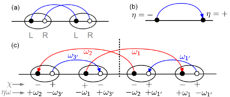
Figure 25: Examples for Liouville space diagrams: (a) two contracted tunneling Liouvillians, (b) Hermitian conjugation indices are expressed by directions of arrows, (c) reading off the propagator for a certain segment (for the segment indicated by the vertical dashed line, we obtain $X_{2}=\omega_{1}-\omega_{2}$). Charge indices $\chi$ are denoted by $+$ or $-$ below the propagator line, the factors $\eta\omega$ appearing in Eq. (256) are denoted are shown for the sake of completeness.

The factor $X_{i}$ of the $i$-th propagator segment can be readily read off from the diagrams as illustrated in Fig. 25: firstly, all energies associated with contractions that connect dots that lie on the same side of this segment do not contribute to $X_{i}$ (cf. Fig. 25 (c), grey contractions). For “later” dots this is clear as they are always excluded in the sum of definition (256). For “earlier” dots the respective energy occurs twice in the sum with opposite sign $\eta_{i}$ (enforced to the contraction (244)). Thus, only the contraction lines that intersect a vertical line drawn at the $i$-th propagator segment contribute to $X_{i}$ (red contractions in Fig. 25 (c)). To determine $X_{i}$ completely, we need to know the h. c. indices $\eta_{i}$, which we will depict by arrows attached to the contraction lines: if a vertex has $\eta_{i}=+(-)$, the arrow points towards (away from) this vertex (see Fig. 25 (b)).

Finally, we indicate the charge index $\chi=\pm$ of every dot in the diagram by a sign below the propagator line (see Fig. 25 (c)). Note that charge indices $\chi$ of a double vertex must be opposite by Eq. (240). Our diagrams therefore represent the algebraic expression associated with both a fixed contraction structure and fixed $(\eta,\chi)$-indices. The latter is a distinction to the Liouville space diagrams used, e.g, in Schoeller (2009): distinct combinations of $(\eta,\chi)$ represent distinct diagrams. Hence, the $n$-th order contribution $\langle A\rangle_{n}$ to the expectation value of $A$ is represented by a set of diagrams covering all allowed combinations contractions and all combinations for $(\eta,\chi)$’s.

For the ensuing discussion, we will first ignore any sign factors in $\langle A\rangle_{n}(z)$, for example due to the contraction functions. This discussion and the question which diagrams are allowed is most conveniently postponed to the very end of our derivations.

E.4 Energy-Spin Separation

We now arrive at the crucial part of the derivation of covariant diagram rules: the separation of the spin-dependent and energy-dependent parts in $\Sigma_{A}^{\mathrm{irr}}(i0)$ and recasting the former as a trace in spin space similar to Sec. A.2. For the sake of simplicity, we first replace the observable vertex by a tunneling vertex and discuss modifications afterwards.

In Eq. (255), we have three different spin-dependent factors: (i) the energies $\varepsilon_{i}=\varepsilon_{n_{i}k_{i}\sigma_{i}}^{r_{i}}$, (ii) the contractions $\gamma_{ij}\propto\delta_{\sigma_{i}\sigma_{j}}$ and (iii) the tunneling amplitudes $t_{\sigma\sigma^{\prime}}$.

(i)+(ii): Any pair of contracted indices, say $i$ and $j$ occur in  Eq. (255) with a sum of the form

$$\sum_{n_{i},k_{i}}\delta_{\sigma_{i}\sigma_{j}}g(\varepsilon_{n_{i}k_{i}\sigma_{i}}^{r_{i}}),$$ (257)

where $g$ is some function of $\varepsilon^{r_{i}}_{n_{i}k_{i}\sigma_{i}}=\varepsilon^{r_{j}}_{n_{j}k_{j}\sigma_{j}}$. We can get rid of the spin-dependence of the energies by introducing the spin-dependent DOS, proceeding analogous to the derivation of Eq. (46). Eq. (257) then equals

$$\int d\omega_{i}\bar{\nu}^{r_{i}}(\omega_{i})g(\omega_{i})\left[\text{}_{r_{i}}\langle\sigma_{i}|\check{\mathbf{r}}\cdot\check{\mathbf{n}}^{r_{i}}(\omega_{i})|\sigma^{\prime}\rangle_{r_{i}}\right]^{\bar{\eta}_{i}}.$$ (258)

The scalar product now involves a new 4-vector with $\check{\mathbf{n}}(\omega)=\sqrt{2}\left(1,n^{r}(\omega)\hat{\mathbf{J}}^{r}\right)$. Furthermore, we artificially introduced the complex conjugation by $\bar{\eta}$ even though the matrix elements $\text{}_{r}\langle\sigma|\check{\mathbf{r}}\cdot\check{\mathbf{n}}^{r}(\omega)|\sigma^{\prime}\rangle_{r}$ are real. This will become advantageous for later manipulations. We therefore simply replace $\varepsilon_{i}$ by $\omega_{i}$ in Eq. (255) and the sum over the index $i$ now abbreviates also an integration over $\omega_{i}$ instead of a summation over $n_{i},k_{i}$.

(iii): The spin-dependence of the tunneling amplitudes can be rewritten as a matrix element in spin space, too:

$${}[T^{LR}_{\sigma\sigma^{\prime}}]^{\eta^{\prime}} = \left[\text{}_{L}\langle\sigma|\check{\mathbf{t}}\cdot\check{\mathbf{r}}|\sigma^{\prime}\rangle_{R}\right]^{\eta^{\prime}}.$$ (259)

We next separate the frequency dependent parts (propagators, Fermi functions, $\check{\mathbf{t}}$ and $\check{\mathbf{n}}$-vectors) and the spin-dependent matrix elements, which leads to

$$A|_{n} = \sum_{\{\kappa,\rho,\omega_{i}\}}(\mathrm{signs})(\mathrm{prop}.)\left[\ldots\check{t}_{\kappa_{i}}\ldots\frac{(\check{F}_{i})_{\rho_{i}}}{\pi}\ldots\right]$$ (260)

$$\times\sum_{\{\sigma\}}\left(\ldots(\check{r}_{\kappa_{i}})^{\eta_{i^{\prime}}}_{\sigma_{i}\sigma_{i^{\prime}}}\ldots(\check{r}_{\rho_{i}})^{\bar{\eta}_{\sigma_{k^{\prime}}}}_{\sigma_{k}\sigma_{k^{\prime}}}\ldots\right).$$

The sum over the $\kappa_{i}$’s and $\rho_{i}$’s indicates the scalar products of the respective 4-vectors with the matrix elements $(\check{r}_{\mu})_{\sigma_{i}\sigma_{i^{\prime}}}$ of the charge-spin operator $\check{r}_{\mu}$. For simplicity, we do not indicate here the quantization axis for the basis states used to express these matrix elements since we will see below that this choice drops our. We moreover introduced the abbreviation

$$(F_{i})_{\rho_{i}} = \bar{\nu}^{r_{i}}(\omega_{i})\check{n}_{\rho_{i}}^{r_{i}}(\omega_{i})f^{r_{i}}_{\bar{\chi}_{i}}(\omega_{i}).$$ (261)

Interestingly, the sum over the spin indices factorizes into sums over the spin indices of vertices that are connected in the diagrams in a loop (when formally considering contraction lines to be connected at each double vertex, cf. Fig. 25 (c), which consists of a single loop). The contribution of each loop can be evaluated independently as follows: if we start at an arbitrary dot and follow the directed contraction line. For every loop element we encounter (vertex, contraction), we put charge-spin operators in a sequence from the right to the left into a trace. For example, starting at the dot labelled 1’ in Fig. 25 (c), we obtain the expression $\mathrm{tr}(\check{r}_{\kappa_{1^{\prime}}}\check{r}_{\rho_{1}}\check{r}_{\kappa_{3^{\prime}}}\check{r}_{\rho_{3^{\prime}}}\check{r}_{\kappa_{4^{\prime}}}\check{r}_{\rho_{2}}\check{r}_{\kappa_{2^{\prime}}}\check{r}_{\rho_{1^{\prime}}})$. Thus, Eq. (260) becomes

$$A|_{n} \sim (\mathrm{signs})\int_{\{\omega_{i}\}}(\mathrm{propagators})$$ (262)

$$\times\prod_{\mathrm{loops}}\mathrm{tr}\left[\ldots\left(\check{\mathbf{t}}\cdot\check{\mathbf{r}}\right)\ldots\left(\mathbf{F}_{i}\cdot\check{\mathbf{r}}\right)\ldots\right],$$

where we moved the frequency-dependent 4-vectors $\mathbf{t}$ and $\mathbf{F}_{i}$ into the spin traces and restored the scalar products.

The rest of this section is dedicated to prove this simple rule. We therefore start from the sequence of matrix elements $\check{r}_{\sigma\sigma^{\prime}}$, obtained by writing them down from the right to the left in the order in which we encounter down when following a directed loop. We have to prove that pairs of the same spin indices are next to each other when we change all Hermitian conjugation indices of the matrix elements in to in Eq. (260) to + (except for the left- and right-most one), so that the expression can be recast as a trace. We will suppress the $\mu$-indices for convenience and we let $\sigma_{\mathrm{prec}}$ denote a spin index of the preceding element we have already run through and $\sigma_{\mathrm{succ}}$ will refer to a spin index of the succeeding loop element. We have to insert the following factors:

(i) For each contraction, put a factor $\check{r}^{\bar{\eta}_{\mathrm{early}}}_{\sigma_{\mathrm{late}}\sigma_{\mathrm{early}}}$ where $\eta_{\mathrm{early}}$ is the h. c. index of the earlier vertex involved. We first note that the h. c. index $\eta_{i}$ of the vertex $i$ at which we start to follow a contraction line has always $\eta_{i}=-$ (the arrow points away from the vertex). We have to distinguish two cases: (ia) if we start at the early vertex (e. g. contraction $1^{\prime}$ in Fig. 11), we have $\eta_{\mathrm{early}}=-$ and thus $\begin{array}[]{lll}\check{r}^{\bar{\eta}_{\mathrm{early}}}_{\sigma_{\mathrm{late}}\sigma_{\mathrm{early}}}&=&\check{r}^{+}_{\sigma_{\mathrm{succ}}\sigma_{\mathrm{prec}}}\end{array}$whence in case (ib) we start at the late vertex (e. g. contraction $1$ in Fig. 25 (c)), so $\eta_{\mathrm{early}}=+$ and thus $\begin{array}[]{lll}\check{r}^{\bar{\eta}_{\mathrm{early}}}_{\sigma_{\mathrm{late}}\sigma_{\mathrm{early}}}&=&\check{r}^{-}_{\sigma_{\mathrm{prec}}\sigma_{\mathrm{succ}}}=\check{r}^{+}_{\sigma_{\mathrm{succ}}\sigma_{\mathrm{prec}}}\end{array}$, using the Hermiticity of the Pauli matrices.

(ii) For each double vertex, we put a factor $\check{r}^{\eta_{\mathrm{early}}}_{\sigma_{\mathrm{late}}\sigma_{\mathrm{early}}}$. Again, there two cases: (a) if $\eta_{\mathrm{early}}=+$, we arrive at the earlier vertex, so we have $\begin{array}[]{lll}\check{r}^{\eta_{\mathrm{early}}}_{\sigma_{\mathrm{late}}\sigma_{\mathrm{early}}}&=&\check{r}^{+}_{\sigma_{\mathrm{succ}}\sigma_{\mathrm{prec}}}\end{array}$ (e. g., later double vertex in Fig. 25 (c)) whence (b) if $\eta_{\mathrm{early}}=-$ (e. g. earlier vertex in Fig. 25 (c)), we arrive at the later vertex, so we have $\begin{array}[]{lll}\check{r}^{\eta_{\mathrm{early}}}_{\sigma_{\mathrm{left}}\sigma_{\mathrm{right}}}&=&\check{r}^{-}_{\sigma_{\mathrm{prec}}\sigma_{\mathrm{succ}}}=\check{r}^{+}_{\sigma_{\mathrm{succ}}\sigma_{\mathrm{prec}}}\end{array}$. These considerations prove the simple rule:

$$\sum_{\{\sigma_{i},\sigma_{i^{\prime}}\}}\check{r}^{+}_{\sigma_{n}\sigma_{n^{\prime}}}\ldots\check{r}^{+}_{\sigma_{1}\sigma_{1^{\prime}}}\check{r}^{+}_{\sigma_{1^{\prime}}\sigma_{n}} = \mathrm{tr}(\check{r}\ldots\check{r}).$$ (263)

Here we used that the matrix elements of adjacent Pauli operators are taken for spin states with respect to the same quantization axis, i. e., we can combine $\sum_{\sigma_{1^{\prime}}}\check{r}^{+}_{\sigma_{1}\sigma_{1^{\prime}}}\check{r}^{+}_{\sigma_{1^{\prime}}\sigma_{n}}=\text{}_{r_{1}}\langle\sigma_{1}|\hat{r}|\sigma_{1^{\prime}}\rangle_{r_{1}^{\prime}}\text{}_{r_{1}^{\prime}}\langle\sigma_{1^{\prime}}|\hat{r}|\sigma_{n}\rangle_{r_{n}}=\text{}_{r_{1}}\langle\sigma_{1}|\hat{r}\hat{r}|\sigma_{n}\rangle_{r_{n}}$ and so on.

E.5 Sign Factors

Having tackled the most tedious part, the spin and energy dependence, it remains to collect all sign factors of an expression from its representing diagram, yielding

$$\mathrm{signs} = (-1)^{\text{\#cr.}}\prod_{\begin{subarray}{c}\mathrm{\mathrm{early}+\mathrm{late}}\\ \mathrm{\mathrm{vertices}}\end{subarray}}\chi_{e}\prod_{\begin{subarray}{c}\mathrm{\mathrm{intermediate}}\\ \mathrm{\mathrm{vertices}}\end{subarray}}\eta_{e}.$$ (264)

Here #cr. is the number of crossing contractions lines and “$e$” always refers to the earlier vertex of each double vertex. The meaning of early / intermediate / late vertices is depicted in Fig. 26 and explained in the proof of Eq. (264).

To prove Eq. (264), we first note that there are three origins for signs: (i) an overall permutation factor $(-1)^{N_{p}}$from Wick’s theorem (242), (ii) a factor $(-\chi_{\mathrm{early}}\eta_{\mathrm{early}})$ for every contraction (see Eq. (244)) and (iii) a factor $(-\chi_{\mathrm{early}})$ for every double vertex  (see Eq. (240)). (i) is readily obtained from the  number of crossing contraction lines in the diagrams, giving the first factor of Eq. (264). The signs due to (ii) and (iii) can be determined together: first of all, the minus signs can be omitted since the number of contractions and double vertices is always even. For the further procedure, it is helpful to distinguish three types of vertices sketched in Fig. 26: (a) “late double vertices” where both vertices are the later ones in their contractions. Then no signs due to contractions have to be considered and only the charge index of the earlier vertex occurs. We furthermore have (b) “early double vertices” where both vertices are the earlier ones in their contractions. The signs due to both contractions cancel each other since charge and h. c. indices of both vertices in any double vertex are opposite. Thus, the sign for this type of vertex is again given by the earlier charge index. Finally, there are (c) “intermediate double vertices” where one of the vertices is earlier and the other one is later in its contraction. The sign factor is in this case the h. c. index $\eta_{\mathrm{early}}$ of the earlier vertex of the double vertex.

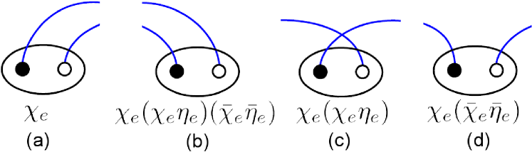
Figure 26: Different types of vertices: late double vertex (a), early double vertex (b) and intermediate double vertices (c), (d). The corresponding sign factors are denoted below the vertex. Note that $\chi_{e},\eta_{e}$ refer to the earlier vertex of the double vertex and not to being earlier in the contractions.

E.6 Hermitian Conjugated Partner Diagrams

Since any observable must have a real expectation value, the imaginary parts of all diagrams have to cancel each other. In fact diagrams come in complex conjugates pairs, which are obtained from each other by inverting the h. c. indices, or, diagrammatically speaking, by inverting all arrow directions. Therefore, it is sufficient to take only one diagram as a representative of both. We therefore obtain schematically instead of Eq. (262)

$$A|_{n} \sim 2\mathrm{Re}(\mathrm{signs})\int_{\{\omega_{i}\}}(\mathrm{propagators})$$ (265)

$$\times\prod_{\begin{subarray}{c}\mathrm{\mathrm{oriented}}\\ \mathrm{\mathrm{loops}}\end{subarray}}\mathrm{tr}\left[\ldots\left(\check{\mathbf{t}}\cdot\check{\mathbf{r}}\right)\ldots\left(\mathbf{F}_{i}\cdot\check{\mathbf{r}}\right)\ldots\right].$$

We will next explicitly show how the complex-conjugation symmetry arises in our formulation of real-time diagrammatics. Inverting all h. c. indices, $\eta_{i}\rightarrow\bar{\eta}_{i}$, involves the following modifications:

(i) The sign factor is negated. All charge indices may be kept fixed except for those of the current vertex (see Eq. (269)). This involves an additional minus sign from the early and late double vertices. The sign due to the intermediate vertices does not change since the number $\#\mathrm{IV}$ of this type of vertices is always even. Reverting all $\eta_{e}\rightarrow\bar{\eta}_{e}$ therefore results in an additional factor $(-1)^{\#\mathrm{IV}}=1$ compared to the original sign factor.

(ii) The order of the Pauli operators in the spin trace is inverted, yielding the complex conjugate of the original trace expression:

$$\mathrm{tr}(\check{r}_{1}\ldots\check{r}_{n}) \rightarrow \mathrm{tr}(\check{r}_{n}\ldots\check{r}_{1})=\mathrm{tr}(\check{r}_{1}\ldots\check{r}_{n})^{\ast},$$ (266)

where we used $\check{r}_{1}^{{\dagger}}=\check{r}_{1}$ and $(\check{r}_{n}^{{\dagger}}\ldots\check{r}_{1}^{{\dagger}})=(\check{r}_{1}\ldots\check{r}_{n})^{{\dagger}}$.

(iii) The propagators are mapped onto their negative Hermitian conjugate since  $X_{i}\rightarrow-X_{i}$

$$\frac{1}{i0+X_{i}} \rightarrow \frac{1}{i0+(-X_{i})}=-\left(\frac{1}{i0+X_{i}}\right)^{\ast}.$$ (267)

As the number of propagators is odd, we obtain an additional minus sign.

Since all remaining factors are real (cf. Eq. (262)) and have no further $\eta$-dependence, we conclude that the mapping $\eta_{i}\rightarrow\bar{\eta}_{i}$ results in the positive complex conjugate contribution of the initial expression. Adding both these partner diagrams gives two times the real part of one of the two diagrams, proving Eq. (265)

E.7 Covariant Diagram Rules for Charge and Spin Current

We first describe the modifications of the covariant diagram rules required for the charge and spin current, which can be treated simultaneously as outlined in IV.1. The expressions for the current operator read (see Eq. (86)):

$$I_{R^{r}_{\mu}} = \sum_{nn^{\prime}kk^{\prime}\sigma\sigma^{\prime}}(-ir_{\mu}T)^{r\bar{r}}_{\sigma\sigma^{\prime}}c^{{\dagger}}_{rnk\sigma}c_{\bar{r}n^{\prime}k^{\prime}\sigma^{\prime}}-\text{h.c.}$$ (268)

with $(rT)_{\sigma\sigma^{\prime}}=\sum_{\tau}r_{\sigma\tau}T^{r\bar{r}}_{\tau\sigma^{\prime}}$. The structure of the current is very similar  to the tunneling Hamiltonian with the simple replacement $T_{\sigma\sigma^{\prime}}^{r\bar{r}}\rightarrow(-ir_{\mu}T)^{r\bar{r}}_{\sigma\sigma^{\prime}}$. Introducing a superoperator for the left action $\mathcal{I}_{R^{r}_{\mu}}\cdot=I_{R^{r}_{\mu}}\cdot$, we may therefore treat the corresponding current vertices similar to the tunneling Liouvillian by making the replacement

$$\bar{\chi}_{1^{\prime}}\left[\text{}_{L}\langle\sigma_{1}|\check{\mathbf{t}}\cdot\check{\mathbf{r}}|\sigma_{1^{\prime}}\rangle_{R}\right]^{\eta_{1^{\prime}}}$$ (269)

$$\rightarrow \delta_{\bar{\chi}_{1^{\prime}}\eta_{1^{\prime}},+}[(-i)\text{}_{L}\langle\sigma_{1}|i_{R^{r}_{\mu}}|\sigma_{1^{\prime}}\rangle_{R}]^{\eta_{1^{\prime}}}$$

with $i_{R^{r}_{\mu}}$ given by Eq. (274) below. The restriction $\delta_{\bar{\chi}_{1^{\prime}}\eta_{1^{\prime}},+}$ is due to the fact that all field operators in $\mathcal{I}_{R^{r}_{\mu}}$ act from the left whereas the tunneling Liouvillian as a commutator also possesses a part that acts from the right. Consequently, we have account for the following modifications:

(i) Insert $i_{R^{r}_{\mu}}$ instead of $\left(\check{\mathbf{t}}\cdot\check{\mathbf{r}}\right)$ into the spin traces.

(ii) Set $\eta_{1^{\prime}}=\bar{\chi}_{1^{\prime}}=+$. The first equality follows from the factor $\delta_{\bar{\chi}_{1^{\prime}}\eta_{1^{\prime}},+}$ in Eq. (269) and the second from the freedom to chose one representative of the complex conjugated diagrams, which we fix by an explicit choice for $\eta_{1^{\prime}}$. Note that the “missing” factor $\bar{\chi}_{1^{\prime}}=+$ in the second line of Eq. (269) does give any further modifications for this choice.

(iii) Replace $\mathrm{Re}(\ldots)\rightarrow\mathrm{Im}(\ldots)$ in Eq. (265), which is due to the additional factor $(-i)^{\eta_{1^{\prime}}=+}=-i$ in Eq. (269).

We now present a systematic way to draw all diagrams and read off the respective $n$-th order contributions to the expectation value $I_{R^{r}_{\mu}}|_{n}$, schematically given by

$$I_{R^{r}_{\mu}}|_{n} \sim \underset{\begin{subarray}{c}\mathrm{\mathrm{irr}.\mathrm{contr}.}\\ \mathrm{\{\chi,\eta\}}\end{subarray}}{\sum}2\mathrm{Im}\left\{(\mathrm{signs})\int_{\{\omega_{i}\}}\left(\text{...}\frac{1}{i0+X_{i}}\ldots\right)\prod_{\mathrm{loops}}\mathrm{tr}\left[\ldots\left(\check{\mathbf{t}}\cdot\check{\mathbf{r}}\right)\ldots\left(\mathbf{F}_{i}\cdot\check{\mathbf{r}}\right)\ldots\right]\right\}.$$ (270)

The first sum in Eq. (270) adds up all possible diagrams, whereas the residual term corresponds to an individual diagram. All allowed diagrams contributing to $I_{R^{r}_{\mu}}|_{n}$ are obtained by the following drawing instructions (an easy example is given in Fig. 25 (c)).

1. Propagator and vertices. For the $n$-th order contribution, put $n$ double vertices on a propagator line. The later (earlier) vertex of each double vertex refers to the left (right) electrode. Mark the latest vertex with the symbol $I_{R^{r}_{\mu}}$ designating this one to be the observable vertex. Symbol: a horizontal line represents the propagator line; double dots, encircled by a line depict the double vertices; full (empty) dots refer to the left (right) electrode.

2. Contractions. Construct all possible irreducible contractions. Full (empty) vertices are only permitted to be contracted with full (empty) vertices. Symbol: contractions depicted full lines above the propagator; attach an “$i$”, denoting the Liouville index of the earlier dot in each contraction.

3. Hermitian Conjugation Indices. Construct all possibilities for the choice of the h. c. indices, obeying the following rules: (i) the h. c. of one double vertex have to be opposite, (ii) the earlier h. c. index of the observable vertex is +, (iii) the h. c. indices have to alternate in each loop. Symbol: Arrow pointing to (away from) a dot is associated with $\eta=+$ ($\eta=-$).

4. Charge indices. Construct all possible charge index arrangements, restricted by (i) the charge indices of a double vertex have to be opposite, (ii) the charge indices of  the observable vertex have to be opposite to the h. c. indices. Symbol: +,– below the vertex

Translating diagrams into algebraic expressions, schematically indicated in Eq. (270), proceeds as follows:

1. Propagators: For each propagator segment following a tunneling vertex write down a factor

$$\frac{1}{i0+X} X=\sum(\omega_{\mathrm{early}}-\omega_{\mathrm{late}}).$$ with (271)

The sum in $X$ involves all frequencies associated with contractions that cross over that segment from the left to the right (earlier frequency) or from the right to the left (later frequency), respectively.

2. Loopwise evaluation of spin traces: Start at any point and follow the loop in direction of the arrow. Insert from the right to the left into a trace in spin space the following terms when encountering

- a tunneling vertex: $\check{\mathbf{t}}\cdot\check{\mathbf{r}}$,

- an observable vertex:

$$i_{R^{r}_{\mu}} = \left\{\begin{array}[]{ll}-\left(\check{\mathbf{t}}\cdot\check{\mathbf{r}}\right)r_{\mu},&r=R\\ +r_{\mu}\left(\check{\mathbf{t}}\cdot\check{\mathbf{r}}\right),&r=L\end{array}.\right.$$ (274)

- a contraction: $\mathbf{F}_{i}\cdot\check{\mathbf{r}}$ where $i$ refers to the earlier dot, $(F_{i})_{\rho_{i}}=\bar{\nu}^{r_{i}}(\omega_{i})f^{r_{i}}_{\bar{\chi}_{i}}(\omega_{i})\check{n}^{r_{i}}_{\rho_{i}}(\omega_{i})$ and

$$\check{n}^{r}_{\rho}=\sqrt{2}\left\{\begin{array}[]{ll}1&\rho=0\\ n^{r}\hat{J}^{r}_{\rho}&\rho=1,2,3\end{array}.\right.$$ (275)

Repeat this for all other loops in the diagram.

3. Signs: Put a factor

$$(-1)^{\text{\#cr.}}\underset{\begin{subarray}{c}\mathrm{\mathrm{early}+\mathrm{late}}\\ \mathrm{\mathrm{vertices}}\end{subarray}}{\prod}\chi_{e}\underset{\begin{subarray}{c}\mathrm{\mathrm{intermediate}}\\ \mathrm{\mathrm{vertices}}\end{subarray}}{\prod}\eta_{e},$$

where $\#\mathrm{cr}$. is the number of crossings of contractions, the subscript “$e$” refers to the earlier dot of a vertex. For the meaning of late, early and intermediate double vertices, see Fig. 26.

4. Complete expectation value: Multiply all expressions obtained from steps 1, 2 and 3 and integrate over all frequencies $\{\omega_{i}\}$, where $i$ refers to the indices associated with the contractions. Take $2\mathrm{Im}(\ldots)$ of this expression and sum up the contributions of all valid diagrams.

E.8 Covariant Diagram Rules for Spin-quadrupole Current

The calculation of the expectation value of the SQM current requires some modifications compared to that of the charge and spin-dipole current. The reason is that the spin-quadrupole current operator for node $\langle rr^{\prime}\rangle$, i. e. $\bm{\mathcal{I}}^{rr^{\prime}}_{\bm{\mathcal{Q}}}=i\left[H_{T},\bm{\mathcal{Q}}^{rr^{\prime}}\right]$, is a dyadic of two vector operators:

$$\bm{\mathcal{I}}^{rr^{\prime}}_{\bm{\mathcal{Q}}}=\frac{1}{2}\left[g^{rr^{\prime}}\mathbf{I}_{\mathbf{S}^{r}}\odot\mathbf{S}^{r^{\prime}}+(r\leftrightarrow r^{\prime})+h.c.\right].$$ (276)

We remind the reader of the factor $g^{rr^{\prime}}=2$ if $r\neq r^{\prime}$ and $g^{rr}=1$. Crudely speaking, the diagrams for the spin-quadrupole current have the same structure as for the spin current, but include an additional spin vertex. However, the spin operator has to be treated differently from the tunneling or current vertices (268) as is contains only one sum over the $k$-modes (see Eq. (41)) instead of two. We will discuss this point later in detail.

We will restrict ourselves in the following to spin-independent tunneling. If and only if this is the case, we may replace $\mathbf{I}_{\mathbf{S}}^{r}$ by $2\mathbf{I}^{r\bar{r}}_{\mathbf{S}^{r}}$ where

$$\mathbf{I}_{\mathbf{S}^{r}}^{r\bar{r}} = \sum_{k,k^{\prime},\sigma,\sigma^{\prime}}\left[-i\text{}_{r}\langle\sigma|\mathbf{i}_{\mathbf{S}^{r}}|\sigma^{\prime}\rangle_{\bar{r}}\right]c_{rk\sigma}^{{\dagger}}c_{\bar{r}k^{\prime}\sigma^{\prime}}$$ (277)

with $\bar{r}=R,L$ for $r=L,R$ and $\mathbf{i}_{\mathbf{S}^{r}}$ defined in Eq. (274) for $\mu=x,y,z$. Note that $\mathbf{I}_{\mathbf{S}^{r}}^{r\bar{r}}$ only accounts for the contribution to the spin current for electrode $r$ due to tunneling from subsystem $\bar{r}$ to $r$, but not for tunneling from $r$ to $\bar{r}$. Using Eq. (276), the expectation value of the spin-quadrupole current is then given by

$$\langle\bm{\mathcal{I}}^{rr^{\prime}}_{\bm{\mathcal{Q}}}\rangle = 2g^{rr^{\prime}}\mathrm{Re}\,\mathrm{tr}\left(\mathbf{I}_{\mathbf{S}^{r}}^{r\bar{r}}\odot\mathbf{S}^{r^{\prime}}\right)\rho(t)+(r\leftrightarrow r^{\prime}).\,$$ (278)

In the following, we will discuss the modifications that are necessary to calculate Eq. (278) starting from the spin current. First of all, $\bm{\mathcal{I}}_{\bm{\mathcal{Q}}^{rr^{\prime}}}$ contains four field operators so that the associated observable vertex is a quadruple vertex instead of a double vertex. This is sketched in Fig. 27: the later two vertices refer to the spin current operator (whose dots refer to two electrodes) and the earlier vertices refer to the spin operator (whose dots refer to only one electrode). As all field operators act from the left, all charge indices are opposite to the h. c. indices. The action of the spin operator can be expressed by

$$S_{j} \sim \delta_{\eta_{1^{\prime}},+}\delta_{-\eta_{1^{\prime}}\chi_{1^{\prime}},+}\delta_{\chi_{1},\bar{\chi}_{1^{\prime}}}\delta_{\eta_{1},\bar{\eta}_{1^{\prime}}}\delta_{k_{1}k_{1^{\prime}}}(s^{r}_{j})_{\sigma_{1}\sigma_{1^{\prime}}}J_{1}J_{1^{\prime}}.$$

This fixes $\eta_{\mathrm{early}}=\bar{\chi}_{\mathrm{early}}=+$.

Figure 27: SQM current vertex

The technical challenge for implementing the spin-quadrupole current vertex is the single $k$-summation in the spin operator. If we contract the two dots within the spin operator this is no problem since the contraction also sets the $k$-indices to be the same anyway. However, if the two dots are contracted with other vertices, their $k$’s are not independent, so we cannot introduce the one-particle DOS for both contractions individually (denoted by $1$ and $1^{\prime}$ in the following). Instead, we obtain an expression of the form:

$$\sum_{\tau_{1}\tau_{1^{\prime}}}\sum_{k_{1}}\delta_{\sigma_{1}\tau_{1^{\prime}}}\delta_{\sigma_{1^{\prime}}\tau_{1}}g(\varepsilon^{r^{\prime}}_{n_{1}k_{1}\tau_{1^{\prime}}},\varepsilon^{r^{\prime}}_{n_{1}k_{1}\tau_{1}})\text{}^{r^{\prime}}\langle\sigma_{1}|\mathbf{s}|\sigma_{1^{\prime}}\rangle^{r^{\prime}},$$ (280)

where $g$ is some function and the Cartesian index $j$ refers to the spin operator. We may treat this expression similar to the calculation of the exchange contribution to the spin-quadrupole moment in equilibrium (see Sec. II.3) by introducing the two-particle density of states $\nu^{r}_{\sigma_{1}\sigma_{1^{\prime}}}(\omega_{1},\omega_{1^{\prime}})$ (16) and expressing the latter by Eq. (155). Then the term in (280) equals

$$\int_{\{\omega_{1},\omega_{1^{\prime}}\}}g(\omega_{1},\omega_{1^{\prime}})2\bm{\mathcal{A}}^{r^{\prime}}_{\mu\nu}\text{}_{r^{\prime}}\langle\sigma_{1}|\check{r}_{\mu}\mathbf{s}\check{r}_{\nu}|\sigma_{1^{\prime}}\rangle\text{}_{r},$$ (281)

where the 2DOS (16) enters through the matrix $\bm{\mathcal{A}}^{r}_{\mu\nu}$ given by (156)-(159). Consequently, the frequency and energy part of the diagrams can be treated without modification as explained in Sec. E.4. Furthermore, the signs can be treated without modifications as well as we can simply omit the factor $\bar{\chi}_{1^{\prime}}=+$ in Eq. (LABEL:eq:spinVertex). In contrast, the spin-part is altered: we now insert for the spin vertex and the two associated contractions the factor $\sqrt{2}\mathcal{A}^{r}_{\mu\nu}\check{r}_{\mu}s_{j}\check{r}_{\nu}$ into the spin trace.

Finally, we mention that the symmetrization in $r\leftrightarrow r^{\prime}$ and multiplying with $g^{rr^{\prime}}$in Eq. (278) is equivalent to multiplying with a factor of $2$ and symmetrizing in $r\leftrightarrow r^{\prime}$ only for $r\neq r^{\prime}$.

We now summarize the modifications of the diagram rules for the SQM current compared to the spin current. We first state the drawing rules:

1. Propagator and vertices: the observable vertex consists of four vertices, the later two depicting $\mathbf{I}_{\mathbf{S}^{r}}$ and the earlier two depicting $\mathbf{S}^{r^{\prime}}$.

2. Contractions. No changes.

3. Indices. The h. c. indices of the observable vertex are fixed to (–,+,–,+) and the charge indices are opposite to this.

The changes in the rules for translation into algebraic expressions are:

1. Propagators. No changes.

2. Evaluation of loops. If the vertices associated with $\mathbf{S}^{r^{\prime}}$ in Eq. (278) are

(a) contracted with eachoter, then insert $\mathbf{F}_{+}^{r^{\prime}}(\omega_{1^{\prime}})\cdot\check{\mathbf{r}}\mathbf{s}$.

(b) contracted with other vertices, then insert  $2t^{2}f^{r_{1}}_{\bar{\chi}_{1}}(\omega_{1})f^{r_{1^{\prime}}}_{\bar{\chi}_{1}^{\prime}}(\omega_{1^{\prime}})\bm{\mathcal{A}}^{r^{\prime}}_{\mu\nu}\check{r}_{\mu}\mathbf{s}\check{r}_{\nu}$.

This accounts for both the vertices and their contractions. Here 1 (1’) refers to the indices of the contractions of the later (earlier) vertex.

3. Signs. For the evaluation of the signs, treat the SQM current vertex as two double vertices.

4. Complete expectation value. Multiply with a factor of $2$ and retain the symmetric and traceless part of the tensor-valued result $\sim\mathbf{i}_{\mathbf{S}^{r}}\otimes\mathbf{s}$. If $r\neq r^{\prime}$, symmetrize the result in $r\leftrightarrow r^{\prime}$.

References

- M. Julliere (1975) M. Julliere, Phys. Lett. A 54, 225 (1975).
- J. C. Slonczewski (1989) J. C. Slonczewski, Phys. Rev. B 39, 6995 (1989).
- Potok et al. (2002) R. M. Potok, J. A. Folk, C. M. Marcus, and V. Umansky, Phys. Rev. Lett. 89, 266602 (2002).
- Braun et al. (2005) M. Braun, J. König, and J. Martinek, Superlatt. and Microstruct. 37, 333 (2005).
- Schmidt (2005) G. Schmidt, Journal of Physics D: Applied Physics 38 (2005).
- Glazman and Raikh (1988) L. I. Glazman and M. E. Raikh, JETP Lett. 47, 452 (1988), [Pis’ma v ZhETF 47, 378 (1988)].
- Goldhaber-Gordon et al. (1998) D. Goldhaber-Gordon, H. Shtrikman, D. Mahalu, D. Abusch-Magder, U. Meirav, and M. A. Kastner, Nature 391, 156 (1998).
- K. Ono et al. (2002) K. Ono, D. G. Austing, Y. Tokura, and S. Tarucha, Science 297, 1313 (2002).
- Weinmann et al. (1994) D. Weinmann, W. Häusler, W. Pfaff, B. Kramer, and U. Weiss, Eur. Phys. Lett. 26, 467 (1994).
- Chye et al. (2002) Y. Chye, M. E. White, E. Johnston-Halperin, B. D. Gerardot, D. D. Awschalom, and P. M. Petroff, Phys. Rev. B 66, 201301 (2002).
- Braun et al. (2004) M. Braun, J. König, and J. Martinek, Phys. Rev. B 70, 195345 (2004).
- D. Gatteschi and Villain (2006) R. S. D. Gatteschi and J. Villain, Molecular Nanomagnets (OUP Oxford, 2006).
- Brune and Gambardella (2009) H. Brune and P. Gambardella, Surface Science 603, 1812 (2009).
- Sothmann and König (2010) B. Sothmann and J. König, Phys. Rev. B 82, 245319 (2010).
- Baumgärtel et al. (2011) M. M. E. Baumgärtel, M. Hell, S. Das, and M. R. Wegewijs, Phys. Rev. Lett. 107, 087202 (2011).
- Misiorny et al. (2012a) M. Misiorny, M. Hell, and M. R. Wegewijs, submitted (2012a).
- Misiorny et al. (2012b) M. Misiorny, I. Weymann, and J. Barnaś, Phys. Rev. B 86, 245415 (2012b).
- Cottingham and Greenwood (2001) W. N. Cottingham and D. A. Greenwood, An Introduction to Nuclear Physics, vol. 1 (Cambridge University Press, 2001).
- Hell and Wegewijs (2013) M. Hell and M. R. Wegewijs, in preparation (2013).
- Gatteschi and Sessoli (2003) D. Gatteschi and R. Sessoli, Angew. Chem. Int. Ed. 42, 268 (2003).
- J. König and J. Martinek (2003) J. König and J. Martinek, Phys. Rev. Lett. 90, 166602 (2003).
- Misiorny et al. (2011) M. Misiorny, I. Weymann, and J. Barnaś, Phys. Rev. Lett. 106, 126602 (2011).
- May et al. (2011) F. May, M. R. Wegewijs, and W. Hofstetter, Beilstein J. Nanotechnol. 2, 693 (2011).
- Lindell (1992) I. V. Lindell, Methods for electromagnetic field analyisis, IEEE Series on Electromagnetic Wave Theory (IEEE Press, 1992).
- Schoeller (2009) H. Schoeller, Eur. Phys. Journ. B 168, 179 (2009).
- Leijnse and Wegewijs (2008) M. Leijnse and M. R. Wegewijs, Phys. Rev. B 78, 235424 (2008).
- Saptsov and Wegewijs (2012) R. B. Saptsov and M. R. Wegewijs, Phys. Rev. B 86, 235432 (2012).
- Saptsov (2010) R. B. Saptsov, private notes (2010).