Autonomous Spacecraft Navigation With Pulsars

Abstract

An external reference system suitable for deep space navigation can be defined by fast spinning and strongly magnetized neutron stars, called pulsars. Their beamed periodic signals have timing stabilities comparable to atomic clocks and provide characteristic temporal signatures that can be used as natural navigation beacons, quite similar to the use of GPS satellites for navigation on Earth. By comparing pulse arrival times measured on-board a spacecraft with predicted pulse arrivals at a reference location, the spacecraft position can be determined autonomously and with high accuracy everywhere in the solar system and beyond. The unique properties of pulsars make clear already today that such a navigation system will have its application in future astronautics. In this paper we describe the basic principle of spacecraft navigation using pulsars and report on the current development status of this novel technology.

1 Introduction

Today, the standard method of navigation for interplanetary spacecraft is a combined use of radio data, obtained by tracking stations on Earth, and optical data from an on-board camera during encounters with solar system bodies. Radio measurements taken by ground stations provide very accurate information on the distance and the radial velocity of the spacecraft with typical random errors of about 1 m and 0.1 mm/s, respectively (Maddè et al.,, 2006). The components of position and velocity perpendicular to the Earth-spacecraft line, however, are subject to much larger errors due to the limited angular resolution of the radio antennas. Interferometric methods can improve the angular resolution to about 25 nrad, corresponding to an uncertainty in the spacecraft position of about 4 km per astronomical unit (AU) of distance between Earth and spacecraft (James et al.,, 2009). With increasing distance from Earth, the position error increases as well, e.g., reaching a level of uncertainty of the order of $\pm 200$ km at the orbit of Pluto and $\pm 500$ km at the distance of Voyager 1. Nevertheless, this technique has been used successfully to send space probes to all planets in the solar system and to study asteroids and comets at close range. However, it might be necessary for future missions to overcome the disadvantages of this method, namely the dependency on ground-based control and maintenance, the increasing position and velocity uncertainty with increasing distance from Earth as well as the large propagation delay and weakening of the signals at large distances. It is therefore desirable to automate the procedures of orbit determination and orbit control in order to support autonomous space missions.

Possible implementations of autonomous navigation systems were already discussed in the early days of space flight (Battin,, 1964). In principle, the orbit of a spacecraft can be determined by measuring angles between solar system bodies and astronomical objects; e.g., the angles between the Sun and two distant stars and a third angle between the Sun and a planet. However, because of the limited angular resolution of on-board star trackers and sun sensors, this method yields spacecraft positions with uncertainties that accumulate typically to several thousand kilometers. Alternatively, the navigation fix can be established by observing multiple solar system bodies: It is possible to triangulate the spacecraft position from images of asteroids taken against a background field of distant stars. This method was realized and flight-tested on NASA’s Deep-Space-1 mission between October 1998 and December 2001. The Autonomous Optical Navigation (AutoNav) system on-board Deep Space 1 provided the spacecraft orbit with $1\sigma$ errors of $\pm 250$ km and $\pm 0.2$ m/s, respectively (Riedel et al.,, 2000). Although AutoNav was operating within its validation requirements, the resulting errors were relatively large compared to ground-based navigation.

In the 1980s, scientists at NRL (United States Naval Research Laboratory) proposed to fly a demonstration experiment called the Unconventional Stellar Aspect (USA) experiment (Wood,, 1993). Launched in 1999 on the Advanced Research and Global Observation Satellite (ARGOS), this experiment demonstrated a method of position determination based on stellar occultation by the Earth’s limb as measured in X-rays. This technique, though, is limited to satellites in low Earth orbit.

An alternative and very appealing approach to autonomous spacecraft navigation is based on pulsar timing. The idea of using these celestial sources as a natural aid to navigation goes back to the 1970s when Downs, (1974) investigated the idea of using pulsating radio sources for interplanetary navigation. Downs, (1974) analyzed a method of position determination by comparing pulse arrival times at the spacecraft with those at a reference location. Within the limitations of technology and pulsar data available at that time (a set of only 27 radio pulsars were considered), Downs showed that spacecraft position errors on the order of 1500 km could be obtained after 24 hours of signal integration. A possible improvement in precision by a factor of 10 was estimated if better (high-gain) radio antennas were available for the observations.

Chester & Butman, (1981) adopted this idea and proposed to use X-ray pulsars, of which about one dozen were known at the time, instead of radio pulsars. They estimated that 24 hours of data collection from a small on-board X-ray detector with 0.1 m² collecting area would yield a three-dimensional position accurate to about 150 km. Their analysis, though, was not based on simulations or actual pulsar timing analyses; neither did it take into account the technological requirements or weight and power constraints for implementing such a navigation system.

These early studies on pulsar-based navigation estimated relatively large position and velocity errors so that this method was not considered to be an applicable alternative to the standard navigation schemes. However, pulsar astronomy has improved considerably over the last 30 years since these early proposals. Meanwhile, pulsars have been detected across the electromagnetic spectrum and their emission properties have been studied in great detail (cf. Becker, 2009a, , for a collection of comprehensive reviews on pulsar research). Along with the recent advances in detector and telescope technology this motivates a general reconsideration of the feasibility and performance of pulsar-based navigation systems. The present paper reports on our latest results and ongoing projects in this field of research. Its structure is as follows: After summarizing the most relevant facts on pulsars and discussing which pulsars are best suited for navigation purposes in § 2, we briefly describe the principles of pulsar-based navigation in § 3. Pulsars emit broadband electromagnetic radiation which allows an optimization for the best suited waveband according to the highest number of bits per telescope collecting area, power consumption, navigator weight and compactness. A possible antenna type and size of a navigator which detects pulsar signals at 21 cm is described in § 4. In § 5 we discuss the possibility of using X-ray signals from pulsars for navigation. The recent developments of low-mass X-ray mirrors and active-pixel detectors, briefly summarized in § 6, makes it very appealing to use this energy band for pulsar-based navigation.

2 The Various Types of Pulsars and their Relevance for Navigation

Stars are stable as long as the outward-directed thermal pressure, caused by nuclear fusion processes in the central region of the star, and the inward-directed gravitational pressure are in equilibrium. The outcome of stellar evolution, though, depends solely on the mass of the progenitor star. A star like our sun develops into a white dwarf. Stars above $\approx 8$ $\mbox{M}_{\odot}$ undergo a gravitational collapse once their nuclear fuel is depleted. Very massive stars of more than about 30 $\mbox{M}_{\odot}$ end up as black holes and stars in the intermediate mass range of about 8 to 30 $\mbox{M}_{\odot}$ form neutron stars. It is assumed that a neutron star is the result of a supernova explosion, during which the bulk of its progenitor star is expelled into the interstellar medium. The remaining stellar core collapses under its own weight to become a very compact object, primarily composed of neutrons – a neutron star. With a mass of typically 1.4 $\mbox{M}_{\odot}$, compressed into a sphere of only 10 km in radius, they are quasi gigantic atomic nuclei in the universe. Because of their unique properties they are studied intensively by physicists of various disciplines since their discovery in 1967 (Hewish et al.,, 1968).

Fast spinning and strongly magnetized neutron stars are observable as pulsars if their spin axis and magnetic field axis are not aligned. Having co-rotating magnetic fields of $B_{\perp}\approx 10^{9}$–$10^{13}$ G and spin periods down to milliseconds they radiate broadband electromagnetic radiation along narrow emission cones. If this radiation cone crosses the observer’s line of sight a pulse of intensity is recorded in the observing device (cf. Figure 1).

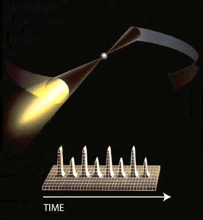
Figure 1: Artist’s impression of a rotation-powered pulsar. The neutron star appears as a pulsating source of radiation if the rotating emission beam crosses the observer’s line of sight. Averaging these periodic pulses of intensity over many rotation cycles results in a stable pulse profile. Because of the timing stability of most pulsars, the arrival time of pulses can be predicted with very high precision, which is an essential requirement for a navigation system based on pulsar observations.

The name Pulsar refers to this property. They have been discovered by their radio signals (Hewish et al.,, 1968). In source catalogs their common abbreviation is therefore PSR which stands for Pulsating Source of Radio, although they have also been detected in other bands of the electromagnetic spectrum meanwhile. Three different classes of pulsars can be distinguished according to the energy source of their electromagnetic radiation. As we will see, only one class is suitable for spacecraft navigation:

• Accretion-powered pulsars are close binary systems in which a neutron star is accreting matter from a companion star, thereby gaining energy and angular momentum. There are no radio waves emitted from the accretion process, but these systems are bright in X-rays. The observed X-ray pulses are due to the changing viewing angle of a million degree hot spot on the surface of the neutron star. These hot spots are heated by in-spiraling matter from an accretion disk. The accretion disk and the accretion column itself can also be sources of X-rays. The spin behavior of accretion-powered pulsars can be very complicated and complex. They often show an unpredictable evolution of rotation period, with erratic changes between spin-up and spin-down as well as X-ray burst activities (Ghosh,, 2007). Although accretion-powered pulsars are usually bright X-ray sources, and thus would give only mild constraints on the sensitivity requirements of a pulsar-based navigation system, their unsteady and non-coherent timing behavior disqualifies them as reference sources for navigation.

• Magnetars are isolated neutron stars with exceptionally high magnetic dipole fields of up to $10^{15}$ G. All magnetars are found to have rotation periods in the range of about 5 to 10 seconds. RXTE and other X-ray observatories have detected super-strong X-ray bursts with underlying pulsed emission from these objects. According to the magnetar model of Duncan & Thompson, (1992), their steady X-ray emission is powered by the decay of the ultra-strong magnetic field. This model also explains the X-ray burst activity observed from these objects, but there are also alternative theories, which relate these bursts to a residual fall-back disk (Trümper et al.,, 2010, 2013). However, their long-term timing behavior is virtually unknown, which invalidates these sources for the use in a pulsar-based spacecraft navigation system.

Concerning their application for navigation, the only pulsar class that really qualifies is that of rotation-powered ones.

• Rotation-powered pulsars radiate broadband electromagnetic radiation (from radio to optical, X- and gamma-rays) at the expense of their rotational energy, i.e., the pulsar spins down as rotational energy is radiated away by its co-rotating magnetic field. The amount of energy that is stored in the rotation of the star can be estimated as follows: A neutron star with a radius of $R=10$ km and a mass of $M=1.4$ $\mbox{M}_{\odot}$ has a moment of inertia $I\approx(2/5)\,M\,R^{2}\approx 10^{45}\,\mbox{g cm}^{2}$. The rotational energy of such a star is $E_{\text{rot}}=2\pi^{2}\,I\,P^{-2}$. Taking the pulsar in the Crab nebula with $P\approx 33$ ms as an example, its rotational Energy is $E_{\text{rot}}\approx 2\times 10^{49}\,\mbox{erg}$, which is comparable with the energy released by thermonuclear burning of our sun in hundred million years. The spin period of a rotation-powered pulsar increases with time due to a braking torque exerted on the pulsar by its magneto-dipole radiation. For the Crab pulsar, the observed period derivative is $\dot{P}=4.2\times 10^{-13}$ s s^-1, which implies a decrease in rotational energy of $\dot{E}_{\text{rot}}=-4\pi^{2}I\,\dot{P}\,P^{-3}\approx 4.5\times 10^{38}\,\mbox{erg s}^{-1}$. It has been found, though, that the spin-down energy is not distributed homogeneously over the electromagnetic spectrum. In fact, only a fraction of about $(10^{-7}-10^{-5})\,\dot{E}_{\text{rot}}$ is observed in the radio band whereas it is roughly $(10^{-4}-10^{-3})\,\dot{E}_{\text{rot}}$ in the X-ray band and $(10^{-2}-10^{-1})\,\dot{E}_{\text{rot}}$ in the gamma-ray band (Becker, 2009b, ).

  There are two types of rotation-powered pulsars: (1) Field pulsars have periods between tens of milliseconds to several seconds and constitute more than 90% of the total pulsar population. (2) About 10% of the known pulsars are so-called millisecond pulsars, which are defined to have periods below 20 milliseconds. They are much older than normal pulsars, posses weaker magnetic fields and, therefore, relatively low spin-down rates. Accordingly, they exhibit very high timing stabilities, which are comparable to atomic clocks (Taylor,, 1991; Matsakis et al.,, 1997). This property of millisecond pulsars is of major importance for their use in a pulsar-based navigation system. Figure 2 clearly shows

  

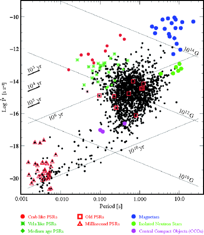
  Figure 2: The $P$-$\dot{P}$ diagram; distribution of rotation-powered pulsars according to their spin parameters. X-ray detected pulsars are indicated by colored symbols. The straight lines correspond to constant ages $\tau=P/(2\dot{P})$ and magnetic field strengths $B_{\perp}=3.2\times 10^{19}(P\dot{P})^{1/2}$ as deduced within the framework of the magnetic braking model.

  that these two types of pulsars belong to distinct populations. Most likely, they are connected by an evolutionary process: It is assumed that millisecond pulsars are born as normal pulsars in a close binary system, but their rotation accelerates as they pass through a phase of accretion in which mass and angular momentum are transferred from the evolving companion star to the pulsar (e.g., Bhattacharya & van den Heuvel,, 1991). However, the fact that millisecond pulsars are often found in binary systems does not affect their suitability for spacecraft navigation as the binary motion can easily be accounted for in pulsar timing (Blandford & Teukolsky,, 1976). Millisecond pulsars – also referred to as recycled pulsars – were discovered by Backer et al., (1982) and studied extensively in the radio band by, e.g., Kramer et al., (1998). Pulsed X-ray emission from millisecond pulsars was discovered by Becker & Trümper, (1993) using ROSAT. However, only XMM-Newton and Chandra had the sensitivity to study their X-ray emission properties in the $0.5-10$ keV band in greater detail. The quality of data from millisecond pulsars available in the X-ray data archives, though, is still very inhomogeneous. While from several of them high quality spectral, temporal and spatial information is available, many others, especially those located in globular clusters, are detected with just a handful of events, not allowing, e.g., to constrain their timing and spectral properties in greater detail. From those millisecond pulsars detected with a high signal-to-noise ratio strong evidence is found for a dichotomy of their X-ray emission properties. Millisecond pulsars having a spin-down energy of $\dot{E}\geq 10^{35}$ erg/s (e.g., PSR J0218$+$4232, B1821$-$24 and B1937$+$21) show X-ray emission dominated by non-thermal radiation processes. Their pulse profiles show narrow peaks and pulsed fractions close to 100% (cf. Figure 3). Common for these pulsars is that they show relatively hard X-ray emission, making it possible to study some of them even with RXTE. For example, emission from B1821$-$24 in the globular cluster M28 is detected by RXTE up to $\approx 20$ keV, albeit with limited photon statistics. For the remaining millisecond pulsars the X-ray emission is found to be much softer, and pulse profiles are more sinusoidal. Their typical fraction of pulsed X-ray photons is between 30 and 60%.

  

  
  

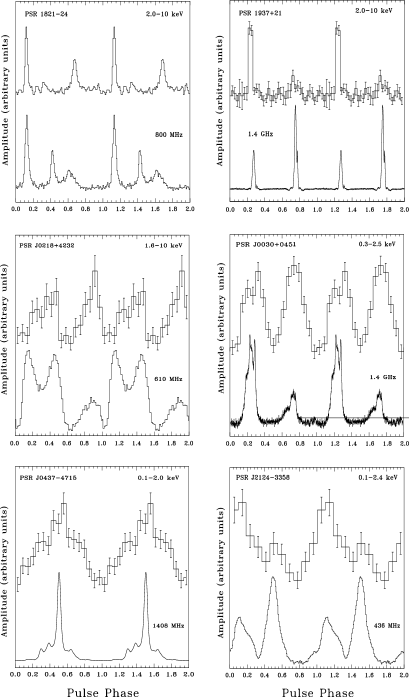
  Figure 3: X-ray and radio pulse profiles for the six brightest millisecond pulsars. Two full pulse cycles are shown for clarity. From Becker, 2009b .

Some rotation-powered pulsars have shown glitches in their spin-down behavior, i.e., abrupt increases of rotation frequency, often followed by an exponential relaxation toward the pre-glitch frequency (Espinoza et al.,, 2011; Yu et al.,, 2013). This is often observed in young pulsars but very rarely in old and millisecond pulsars. Nevertheless, the glitch behavior of pulsars should be taken into account by a pulsar-based navigation system.

Today, about 2200 rotation-powered pulsars are known (Manchester et al.,, 2005). About 150 have been detected in the X-ray band (Becker, 2009b, ), and approximately 1/3 of them are millisecond pulsars. In the past $30-40$ years many of them have been regularly timed with high precision especially in radio observations. Consequently, their ephemerides (RA, DEC, $P$, $\dot{P}$, binary orbit parameters, pulse arrival time and absolute pulse phase for a given epoch, pulsar proper motion etc.) are known with very high accuracy. Indeed, pulsar timing has reached the $10^{-15}$ fractional level, which is comparable with the accuracy of atomic clocks. This is an essential requirement for using these celestial objects as navigation beacons, as it enables one to predict the pulse arrival time of a pulsar for any location in the solar system and beyond.

3 Principles of Pulsar-Based Navigation

The concept of using pulsars as navigational aids is based on measurements of pulse arrival times and comparison with predicted arrival times at a given epoch and reference location. A typical chain for detecting, e.g., radio signals from a rotation-powered pulsar is shown in Figure 4.

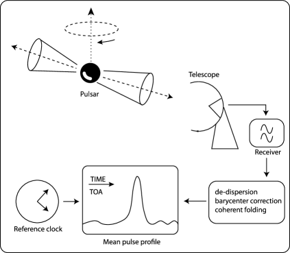
Figure 4: Typical pulsar detection chain. The pulsar beams sweep across the radio antenna. Radio signals are recorded and analyzed in order to produce a mean pulse profile. The data processing comprises a removal of dispersion effects caused by the interstellar medium (“de-dispersion”), correction for the position and proper motion of the observatory (“barycenter correction”) and coherent folding of many pulses. The time of arrival (TOA) of the pulse peak is measured against a reference clock.

An important step in this measurement is the barycenter correction of the observed photon arrival times. The pulsar ephemerides along with the position and velocity of the observer are parameters of this correction. Using a spacecraft position that deviates from the true position during the observation results in a phase shift of the pulse peak (or equivalently in a difference in the pulse arrival time). Therefore, the position and velocity of the spacecraft can be adjusted in an iterative process until the pulse arrival time matches with the expected one. The corresponding iteration chain is shown in Figure 5.

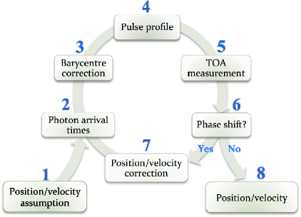
Figure 5: Iterative determination of position and velocity by a pulsar-based navigation system.

An initial assumption of position and velocity is given by the planned orbit parameters of the spacecraft (1). The iteration starts with a pulsar observation, during which the arrival times of individual photons are recorded (2). The photon arrival times have to be corrected for the proper motion of the spacecraft by transforming the arrival times (3) to an inertial reference location; e.g., the solar system barycenter (SSB). This correction requires knowledge of the (assumed or deduced) spacecraft position and velocity as input parameters. The barycenter corrected photon arrival times allow then the construction of a pulse profile or pulse phase histogram (4) representing the temporal emission characteristics and timing signature of the pulsar. This pulse profile, which is continuously improving in significance during an observation, is permanently correlated with a pulse profile template in order to increase the accuracy of the absolute pulse-phase measurement (5), or equivalently, pulse arrival time (TOA). From the pulsar ephemeris that includes the information of the absolute pulse phase for a given epoch, the phase difference $\Delta\phi$ between the measured and predicted pulse phase can be determined (cf. Figure 6).

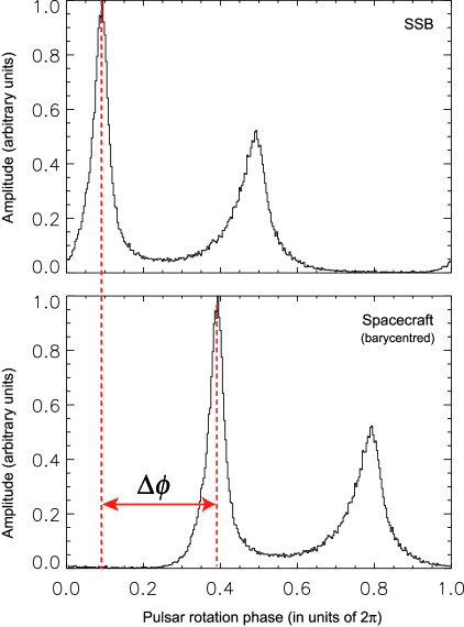
Figure 6: Measuring the phase difference between the expected and measured pulse peak at an inertial reference location; e.g., the solar system barycenter (SSB). The top profile shows the main pulse peak location as expected at the SSB. The bottom profile is the one which has been measured at the spacecraft and transformed to the SSB by assuming the spacecraft position and velocity during the observation. If the position and velocity assumption was wrong, a phase shift $\Delta\phi$ is observed.

In this scheme, a phase shift (6) with respect to the absolute pulse phase corresponds to a range difference $\Delta x=cP(\Delta\phi+n)$ along the line of sight toward the observed pulsar. Here, $c$ is the speed of light, $P$ the pulse period, $\Delta\phi$ the phase shift and $n=0,\pm 1,\pm 2,\ldots$ an integer that takes into account the periodicity of the observed pulses. If the phase shift is non-zero, the position and velocity of the spacecraft needs to be corrected accordingly and the next iteration step is taken (7). If the phase shift is zero, or falls below a certain threshold, the position and velocity used during the barycenter correction was correct (8) and corresponds to the actual orbit of the spacecraft.

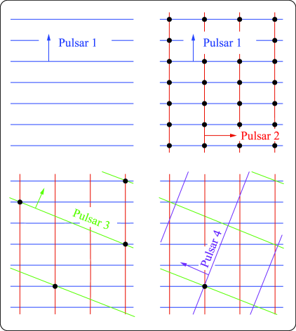
Figure 7: Solving the ambiguity problem by observing four pulsars (drawn in two dimensions). The arrows point along the pulsar’s lines-of-sight. Straight lines represent planes of constant pulse phase; black dots indicate intersections of planes.

A three-dimensional position fix can be derived from observations of at least three different pulsars (cf. Figure 7). If on-board clock calibration is necessary, the observation of a fourth pulsar is required.

Since the position of the spacecraft is deduced from the phase (or pulse arrival time) of a periodic signal, ambiguous solutions may occur. This problem can be solved by constraining the domain of possible solutions to a finite volume around an initial assumed position (Bernhardt et al.,, 2010, 2011), or by observing additional pulsars as illustrated in Figure 7.

4 Radio Antenna for Pulsar-Based Navigation

Pulsars emit broadband electromagnetic radiation. Therefore, the observing device of a pulsar-based navigator can be optimized for the waveband according to the highest number of bits per telescope collecting area, power consumption, navigator weight, cost and compactness. Especially for the question of navigator compactness it is important to estimate what size a radio antenna would have to have in order to detect the emission from pulsars in a reasonable integration time. In order to estimate this we assume pulsar parameters that are typical for millisecond pulsars. As the radio flux from pulsars shows a $\nu^{-1.5}$ dependence, observations at lower frequencies seem to be preferred, but scintillation and scattering effects are stronger at lower frequency. For a navigation system operating in the radio band of the electromagnetic spectrum, the L-band at 21 cm might therefore be best suited.

For a pulsar detection we require a signal-to-noise ratio of $S/N=10$, a minimum integration time of $t_{\text{int}}=3600$ s and assume a frequency bandwidth of $\Delta\nu=100$ MHz. For the receiver noise temperature we take $T_{\text{rec}}=100$ K. A lower temperature would require active, e.g., cryogenic cooling, which would increase cost, weight, and power consumption of a navigator. Furthermore, active cooling would severely limit the lifetime of the navigator due to consumables like helium. For the sky temperature we take $T_{\text{sky}}=5$ K and for the telescope efficiency $\epsilon=0.5$. If $A_{\text{ant}}$ is the geometrical antenna area, the effective antenna area computes as $A_{\text{eff}}=\epsilon\,A_{\text{ant}}$. For the period of the pulsar we assume $P=10$ ms and for the pulse width $W=2$ ms. For the average flux density we adopt $\Delta S=10$ mJy. Using the canonical sensitivity equation (Lorimer & Kramer,, 2005) which corresponds to the radiometer equation applied to pulsar observations

$$\Delta S_{\text{min}}=\frac{2k}{\epsilon A_{\text{ant}}}\frac{(T_{\text{rec}}+T_{\text{sky}})}{\sqrt{n_{p}\,t_{\text{int}}\,\Delta\nu}}\sqrt{\frac{W}{P-W}}$$

and converting it to the geometrical antenna area, including the $S/N$ requirement, we get:

$$A_{\text{ant}}=\frac{S}{N}\frac{2k}{\epsilon\Delta S}\frac{(T_{\text{rec}}+T_{\text{sky}})}{\sqrt{2\,t_{\text{int}}\,\Delta\nu}}\sqrt{\frac{W}{P-W}}$$

Here we have also assumed that both polarizations are averaged ($n_{p}=2$). From this we compute an antenna area of $A_{\text{ant}}\approx 342$ m² for the parameters specified above. For a parabolic antenna it would mean a radius of about $\sqrt{A_{\text{ant}}/\pi}\approx 10.5$ m. Increasing the integration time to 4 hours, we find an area of $\approx 171$ m², which corresponds to a radius of $\approx 7.3$ m. For comparison, the radius of the communication antenna used on Cassini and Voyager is 2 m. It may depend on the satellite platform what size and antenna weight is acceptable, but a parabolic antenna does not seem to be very practical for navigation purposes. A navigator would have to observe several pulsars, either at the same time or in series. The pulsars must be located in different sky regions in order to get an accurate navigation result in the $x$, $y$ and $z$ direction. This, however, means that one either rotates the parabolic antenna or, alternatively, the whole satellite to get the pulsar signals into the antenna focus. Rotating the satellite, though, would mean that the communication antenna will not point to earth any more, which is undesirable. On earth satellites and space missions to the inner solar system, power is usually generated by solar panels. Rotating the satellite would then also mean to bring the solar panels out of optimal alignment with the sun, which is another counter argument for using a parabolic antenna, not to mention the effects of shadowing of the solar panels.

It thus seems more reasonable to use dipole-array antennas for the pulsar observations. Single dipole antennas organized, e.g., as antenna patches could be used to build a larger phased array antenna. Such a phased array would still be large and heavy, though. Depending on the frequency, $10^{4}$–$10^{5}$ single patches are required. There have been no phased-array antennas of that size been build for use in space so far, although smaller prototypes exist (Datashvili et al.,, 2011). From them one may estimate the weight of such antenna arrays. Assuming an antenna thickness of 1 cm and an averaged density of the antenna material of 0.1 g/cm³ still yields an antenna weight of 170 kg for the 170 m² patched antenna array. The signals from the single dipole antennas have to be correlated in phase to each other, which means that all patches have to be connected to each other by a wired mesh and phase correlators. If this phase correlation and the real-time coherent correction for the pulse broadening by interstellar dispersion is done by software, it requires a computer with a Terra-flop GPU of about 500 W power consumption. A clear advantage of a phased antenna array would be that it allows to observe different pulsars located in different sky regions at the same time. That means of course that such an antenna can be smaller if the same $S/N$ ratio is to be achieved for a number $N_{\text{sources}}$ of sources within a given time. With a single-dish antenna one would have to increase its diameter by $N_{\text{sources}}^{1/4}$ if these had to be observed within the same given time interval.

5 Using X-ray Signals from Pulsars for Spacecraft Navigation

The increasing sensitivity of the X-ray observatories ROSAT, RXTE, XMM-Newton and Chandra allowed for the first time to explore in detail the X-ray emission properties of a larger sample of rotation-powered pulsars. The discovery of pulsed X-ray emission from millisecond pulsars (Becker & Trümper,, 1993), the determination of the X-ray efficiency of rotation-powered pulsars (Becker & Trümper,, 1997) as well as discoveries of X-ray emission from various pulsars (e.g., Becker & Trümper,, 1999; Becker et al.,, 2005, 2006) and their detailed spatial, spectral and timing studies are just a few of many accomplishments worth mentioning in this context (e.g., Pavlov et al.,, 2001; Kuiper et al.,, 2002; Weisskopf et al.,, 2004; De Luca et al.,, 2005; Becker, 2009a, ; Hermsen et al.,, 2013). With these new results at hand it was only natural to start looking at their applicability to, e.g., spacecraft navigation based on X-ray data from pulsars. The prospects of this application are of even further interest considering that low-mass X-ray mirrors, which are an important requirement for a realistic implementation of such a navigation system, have been developed for future X-ray observatories.

Given the observational and systematical limitations mentioned above it was a question of general interest, which we found not considered with sufficient gravity in the literature, whether it would be feasible to navigate a spaceship on arbitrary orbits by observing X-ray pulsars.

In order to address the feasibility question we first determined the accuracy that can be achieved by a pulsar-based navigation system in view of the still limited information we have today on pulse profiles and absolute pulse phases in the X-ray band. To overcome the limitations introduced by improper fitting functions, undefined pivot points of pulse peaks and phase shifts by an unmodeled energy dependence in the pulsed signal, we constructed pulse profile templates for all pulsars for which pulsed X-ray emission is detected. Where supported by photon statistics, templates were constructed for various energy ranges. These energy ranges were chosen in order to optimize the $S/N$ ratio of the pulsed signal while sampling as much as possible of the energy dependence of the X-ray pulses.

In the literature various authors applied different analysis methods and often used different definitions for pulsed fraction and pulse peak pivot points. Reanalyzing all data from X-ray pulsars available in the public XMM-Newton, Chandra and RXTE data archives was therefore a requirement to reduce systematic uncertainties that would have been introduced otherwise. The result is a database containing the energy dependent X-ray pulse profiles, templates and relevant timing and spectral properties of all X-ray pulsars that have been detected so far (Prinz,, 2010; Breithuth,, 2012).

According to the harmonic content of an X-ray pulse the templates were obtained by fitting the observed pulse profiles by series of Gaussian and sinusoidal functions. The database further includes information on the local environment of a pulsar, i.e., whether it is surrounded by a plerion, supernova remnant or whether it is located in a crowded sky region like a globular cluster. The latter has a severe impact on the detectability of the X-ray pulses as it reduces the $S/N$ ratio of the pulsed emission by the DC emission from background sources. This in turn is important for the selection of the optimal pulsars that emit pulses, e.g., in the hard band (above $\approx 3$ keV) in order to blend away the softer emission from a supernova remnant or plerion.

The pulse profile templates allow us to measure pulse arrival times with high accuracy even for sparse photon statistics by using a least-square fit of an adequately adjusted template. The error of pulse-arrival-time measurements is dominated by the systematic uncertainty that comes with the limited temporal resolution of the observed pulse profiles used to construct the templates. The statistical error in fitting a measured profile by a template was found to be much smaller in all cases. Assuming that the temporal resolution of the detector is not the limiting factor, the temporal resolution of a pulse profile is given by the widths of the phase bins used to represent the observed X-ray pulse. The bin width, or the number of phase bins applied, is a compromise between maximizing the $S/N$ ratio per phase bin while sampling as much of the harmonic content as possible. Denoting the Fourier-power of the $i$-th harmonic by $R_{i}$ and taking $m$ as the optimal number of harmonics deduced from the H-test (De Jager et al.,, 1989), an exact expression for the optimal number of phase bins is given by $M=2.36(\sum_{i=1}^{m}i^{2}R_{i}^{2})^{1/3}$ (Becker & Trümper,, 1999). This formula compromises between information lost due to binning (i.e., zero bin width to get all information), and the effect of fluctuations due to finite statistics per bin (i.e., bin width as large as possible to reduce the statistical error per bin). The total error (bias plus variance) is minimized at a bin width of $1/M$. We applied this in the reanalysis of pulse profiles in our database. Pulsed fractions were computed by applying a bootstrap method (Becker & Trümper,, 1999), which again leads to results that are not biased by the observers “taste” on where to assume the DC level in a profile.

The minimal systematic phase uncertainty for the pulse profile templates in our database is of the order of 0.001 (Bernhardt et al.,, 2010). This uncertainty multiplied by the rotation period $P$ of the pulsar yields the uncertainty in pulse arrival time due to the limited information we have on the exact X-ray pulse profile. Multiplying this in turn by the speed of light yields the spacecraft’s position error along the line of sight to the pulsar. It is evident by the linear dependence on $P$ that millisecond pulsars are better suited for navigation than those with larger rotation periods.

The precision of a pulsar-based navigation system thus strongly depends on the choice of pulsars and the accuracy of pulse arrival measurements, which is subject to the quality of the available templates, accuracy of the on-board clock and clock calibration. As mentioned above, in order to obtain three-dimensional position information, timing of at least three different pulsars has to be performed. The spatial arrangement of these pulsars is another parameter of the achievable accuracy. Our simulations show that the systematic error of position determination can be reduced significantly by choosing a pulsar triple that is optimal in the sense that the pulsars are nearly perpendicular to each other. Since a pulsar might be obscured by the sun or a planet and, therefore, its availability for navigation depends on the current position of the spacecraft, the optimal pulsar triple has to be selected from a ranking of possible pulsar combinations. The following Table 1 represents the ranking of pulsar combinations, which according to our analysis provide the highest position accuracy via pulsar navigation (Bernhardt et al. 2010).

Rank	Pulsar 3-Combination
1	B1937$+$21	B1821$-$24	J0030$+$0451
2	B1937$+$21	B1821$-$24	J1023$+$0038
3	B1821$-$24	J0030$+$0451	J0437$-$4715
4	B1937$+$21	J1023$+$0038	J0218$+$4232
5	B1821$-$24	J1023$+$0038	J0437$-$4715
6	B1937$+$21	J0030$+$0451	J0218$+$4232
7	B1937$+$21	B1821$-$24	J0437$-$4715
8	B1937$+$21	J0218$+$4232	J0437$-$4715
9	B1821$-$24	J0218$+$4232	J0437$-$4715
10	J1023$+$0038	J0218$+$4232	J0437$-$4715

Table 1: Ranking of pulsar 3-combinations according to the position accuracy achievable when using them in a navigation system based onf X-ray pulsars . All listed sources are solitary millisecond pulsars except J0437$-$4715, which is in a binary.

For the pulsars ranked highest in Table 1 we found position errors of about 5 km as a lower limit (cf. Figure 8). The ranking is independent from a specific spacecraft orbit, but was obtained under the assumption that the navigation system is capable of measuring pulse profiles with the same level of detail and accuracy as the ones used in the simulation. Indeed, this is a severe limitation as those pulse profiles where obtained by powerful X-ray observatories like XMM-Newton and Chandra. It is unlikely, due to weight constraints and power limitations, that a navigation system will have similar capacities in terms of collecting power, temporal resolution and angular resolution.

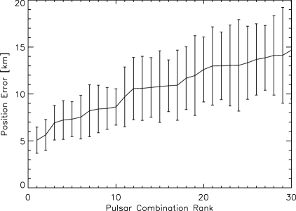
Figure 8: Spacecraft position error as a function of possible pulsar 3-combinations. The diagram shows the mean position errors and standard deviations for the best 30 combinations. From Bernhardt et al., (2010).

An improved accuracy can be achieved by means of pulse profile templates of better quality. This, in turn, calls for deeper pulsar observations by XMM-Newton or Chandra as long as these observatories are still available for the scientific community. It would be a valuable task worthwhile the observing time, especially as it is unclear what missions will follow these great observatories and whether they will provide detectors with sufficient temporal resolution and on-board clock accuracy.

We extended our simulations in order to constrain the technological parameters of possible navigation systems based on X-ray pulsars. The result of this ongoing project will be a high-level design of a pulsar navigator that accounts for boundary conditions (e.g., weight, cost, complexity and power consumption) set by the requirements of a specific spacecraft and mission design.

The chart shown in Figure 9 illustrates the work logic of our current simulations. Navigator boundary conditions (1) and spacecraft orbit (2) are predefined and constrain the technology parameters (3) of the navigator’s X-ray detector, mirror system and on-board electronics. Examples of parameters that will be analyzed in the simulations are detector technology, temporal and energy resolution, on-board-clock accuracy and stability, mirror technology along with collecting power, angular and spatial resolution, focal length, field of view – just to mention the most important ones.

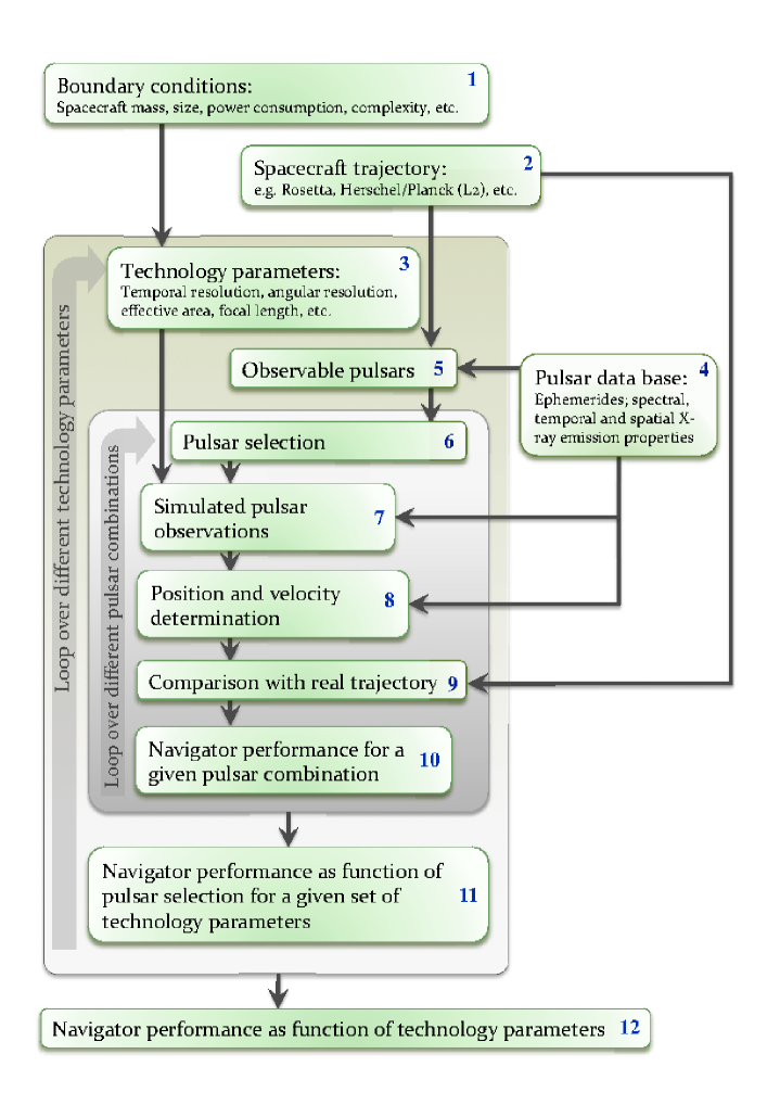
Figure 9: Work flow and logic of the simulations performed for a technology requirement study and demonstrator high-level design of a pulsar-based navigator.

Given their X-ray emission properties some pulsars may not be detectable by the navigator because of its limited angular resolution and sensitivity. The properties of the detector and mirror system along with the trajectory of the virtual navigator thus determine the set of available pulsars (5), from which a suitable selection has to be made (6) according to a predefined ranking of pulsar triples. Using an X-ray-sky simulator (7), which was developed to simulate observations of the future X-ray observatories eROSITA and IXO and which we have modified to include the temporal emission properties of X-ray pulsars, we will be able to create X-ray datasets in FITS-format with temporal, spatial and energy information for the pulsars observed by our virtual navigator. The simulated event files have the same standard FITS-format as those of XMM-Newton and/or Chandra, so that standard software can be used to analyze these data. An autonomous data reduction will then perform the data analysis and TOA measurement in order to obtain the position and velocity of the virtual observer (8). Correlating the result with the input trajectory (9) yields the accuracy of the simulated measurements for a given spacecraft orbit (10), and hence the overall performance of the navigator as a function of the specified detector and mirror system (11,12).

6 X-ray Detector and Mirror Technology for Pulsar-Based Navigation

The design of an X-ray telescope suitable for navigation by X-ray pulsars will be a compromise between angular resolution, collecting area and weight of the system. The currently operating X-ray observatories XMM-Newton and Chandra have huge collecting areas of 0.43 m² and 0.08 m² (at 1 keV), respectively (Friedrich,, 2008, and references therein) and, in the case of Chandra, attain very good angular resolution of less than 1 arcsecond. Their focusing optics and support structures, however, are very heavy. To use their mirror technology would be a show-stopper for a navigation system.

In recent years, ESA and NASA have put tremendous effort into the development of low-mass X-ray mirrors, which can be used as basic technology for future large X-ray observatories and small planetary exploration missions. Table 2 summarizes the angular resolution and mass of X-ray mirrors used for XMM-Newton and Chandra as well as developed for future X-ray missions. The light-weighted mirrors are of special interest for an X-ray pulsar-based navigator.

	Angular	Mass per effective
	resolution	area (at 1 keV)
Chandra	$0.5^{\prime\prime}$	$18\,500$ kg/m2
XMM-Newton	$14^{\prime\prime}$	$2300$ kg/m2
Silicon Pore Optics	$5^{\prime\prime}$	$200$ kg/m2
Glass Micropore Optics	$30^{\prime\prime}$	$25$ kg/m2

Table 2: Comparison of current and future X-ray-mirror optics. From Bavdaz et al., (2010).

A typical high-resolution X-ray telescope uses focusing optics based on the Wolter-I design (Wolter,, 1952). The incoming X-ray photons are reflected under small angles of incidence in order not to be absorbed and are focused by double reflection off a parabolic and then a hyperbolic surface. This geometry allows for nesting several concentric mirror shells into each other in order to enlarge the collecting area and thereby improve the signal-to-noise ratio. A novel approach to X-ray optics is the use of pore structures in a Wolter-I configuration (Bavdaz et al.,, 2003, 2010; Beijersbergen et al., 2004b, ). X-ray photons that enter a pore are focused by reflections on the walls inside the pore. In contrast to traditional X-ray optics with separate mirror shells that are mounted to a support structure, pore optics form a monolithic, self-supporting structure that is lightweight, but also very stiff and contains many reflecting surfaces in a compact assembly. Two different types of pore optics have been developed, based on silicon and glass.

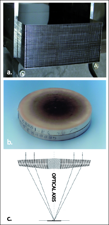
Figure 10: Silicon pore optics (a) and glass micropore optics (b) represent novel developments for light-weighted X-ray mirrors of the next generation of X-ray observatories. Both mirror types will be used in Wolter-I configuration (c) to focus X-rays in a double reflection. Images from Bavdaz et al., (2003, 2004, 2010).

• Silicon Pore Optics (Collon et al.,, 2009, 2010; Ackermann et al.,, 2009) use commercially available and mass produced silicon wafers (Figure 10a) from the semiconductor industry. These wafers have a surface roughness that is sufficiently low to meet the requirements of X-ray optics. A chemo-mechanical treatment of a wafer results in a very thin membrane with a highly polished surface on one side and thin ribs of very accurate height on the other side. Several of these ribbed plates are elastically bent to the geometry of a Wolter-I system, stacked together to form the pore structure and finally integrated into mirror modules (Figure 10a). Silicon Pore Optics are intended to be used on large X-ray observatories that require a small mass per collecting area (on the order of 200 kg/m²) and angular resolution of about 5 arcseconds or better.

• Glass Micropore Optics (Beijersbergen et al., 2004a, ; Collon et al.,, 2007; Wallace et al.,, 2007) are made from polished glass blocks that are surrounded by a cladding glass with a lower melting point. In order to obtain the high surface quality required for X-ray optics, the blocks are stretched into small fibers, thereby reducing the surface roughness. Several of these fibers can be assembled and fused into multi-fiber bundles. Etching away the glass fiber cores leads to the desired micropore structure, in which the remaining cladding glass forms the pore walls (Figure 10b). The Wolter-I geometry is reproduced by thermally slumping separate multi-fiber plates. Glass Micropore Optics are even lighter than Silicon Pore Optics, but achieve a moderate angular resolution of about 30 arcseconds. They are especially interesting for small planetary exploration missions, but also for X-ray timing missions that require large collecting areas. The first implementation of Glass Micropore Optics on a flight program will be in the Mercury Imaging X-ray Spectrometer on the ESA/JAXA mission BepiColombo, planned to launch in 2014 (Fraser et al.,, 2010).

Today’s detector technology, as in use on XMM-Newton and Chandra, is not seen to provide a detector design that is useful for a navigation system based on X-ray pulsars. Readout noise, limited imaging capability in timing-mode and out-of-time events invalidate CCD-based X-ray detectors for application as X-ray-pulsar navigator. Detectors like those on RXTE that need gas for operation are also not suitable, given the limited live time due to consumables. However, there are novel and promising detector developments performed in semiconductor labs for the use in the next generation of X-ray observatories. Two challenging examples, which are of potential interest for navigation, are:

• Silicon Drift Detectors (SDDs) have only limited imaging capability but provide an energy resolution and are capable of managing high counting rates of more than 10 Crab (1 Crab count rate $\approx 200\,000$ cts/s). A detector based on this technology was proposed for the High Time Resolution Spectrometer on IXO (Barret et al.,, 2010). The detector technology itself has a high technical readiness. SDD-modules developed in the Semiconductor Lab of the Max Planck Society are working already in the APXS (Alpha Particle X-ray Spectrometer) on-board NASA’s Mars Exploration Rovers Spirit and Opportunity and on the comet lander ROSETTA (Lechner et al.,, 2010). Detectors based on an SDD technology could be of use, e.g., in designing a navigator for a very specific orbit, for which it is sufficient to navigate according to the signals of pulsars that emit their pulses in the hard X-ray band mostly so that the missing imaging capability does not cause any restrictions on the $S/N$ ratio of the pulsed emission.

• Active Pixel Sensors (APS) are an alternative and perhaps more flexible technology (cf. Figure 11), which was the proposed technology for the Wilde Field Imager on IXO (Strüder et al.,, 2010) and the Low-Energy Detector (LED) on Simbol-X (Lechner,, 2009). This detector provides images in the energy band 0.1–25 keV, simultaneously with spectrally and time resolved photon counting. The device, which is under development in the MPE Semiconductor Laboratory, consists of an array of DEPFET (Depleted p-channel FET) active pixels, which are integrated onto a common silicon bulk. The DEPFET concept unifies the functionalities of both sensor and amplifier in one device. It has a signal charge storage capability and is read out demand. The DEPFET is used as unit cell of Active Pixel Sensors (APSs) with a scalable pixel size from $50\,\mu$m to several mm and a column-parallel row-by-row readout with a short signal processing time of $\leq 4\,\mu$sec per row. As the pixels are individually addressable the DEPFET APS offers flexible readout strategies from standard full-frame mode to user-defined window mode.

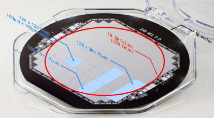
Figure 11: Mechanical sample of an Active Pixel (here 6-inch wafer-scale) detector. Plotted over one hemisphere is the logical layout of the detector. It consists of roughly $1024\times 1024$ pixels of $100\times 100$ $\mu$m² size. From Lechner et al., (2010).

The typical weight and power consumption of these detectors can be estimated from the prototypes proposed for IXO and Simbol-X. The IXO Wide Field Imager with its 17 arcmin field of view and $1024\times 1024$ pixel design had an energy consumption of $\leq 22$ W. The Low Energy Detector on Simbol-X had $128\times 128$ pixels and an energy consumption of $\leq 8$ W. Power consumption including electronics, filter wheel and temperature control was ca. 250 W. The mass of the focal plane, including shielding and thermal interface, was about 15 kg but could be reduced in a more specific design of an X-ray-pulsar navigator.

7 Concluding Remarks

The knowledge of how to use stars, planets and stellar constellations for navigation was fundamental for mankind in discovering new continents and subduing living space in ancient times. It is fascinating to see how history repeats itself in that a special population of stars may play again a fundamental role in the future of mankind by providing a reference for navigating their spaceships through the Universe (cf. Figure 12).

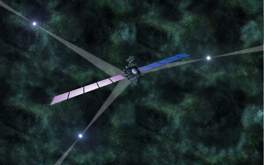
Figure 12: Artist’s impression of Rosetta, if it navigated in deep space using pulsar signals. The characteristic time signatures of pulsars are used as natural navigation beacons to determine the position and velocity of the spacecraft.

In the paper we have shown that autonomous spacecraft navigating with pulsars is feasible when using either phased-array radio antennas of at least 150 m² antenna area or compact light-weighted X-ray telescopes and detectors, which are currently developed for the next generation of X-ray observatories.

Using the X-ray signals from millisecond pulsars we estimated that navigation would be possible with an accuracy of $\pm 5$ km in the solar system and beyond. The error is dominated by the inaccuracy of the pulse profiles templates that were used for the pulse peak fittings and pulse-TOA measurements. As those are known with much higher accuracy in the radio band, it is possible to increase the accuracy of pulsar navigation down to the meter scale by using radio signals from pulsars for navigation.

The disadvantage of radio observations in a navigator, though, is the large size and mass of the phased-antenna array. As we saw in § 4, the antenna area is inversely proportional to the square root of the integration time; i.e., the same signal quality can be obtained with a reduced antenna size by increasing the observation time. However, the observing time is limited by the Allen variance of the receiving system and, therefore, cannot become arbitrarily large. In addition, irradiation from the on-board electronics requires an efficient electromagnetic shielding to prevent signal feedback. This shielding will further increase the navigator weight in addition to the weight of the antenna.

The optimal choice of the observing band depends on the boundary conditions given by a specific mission. What power consumption and what navigator weight might be allowed for may determine the choice for a specific wave band.

In general, however, it is clear already today that this navigation technique will find its applications in future astronautics. The technique behind it is very simple and straightforward, and pulsars are available everywhere in the Galaxy. Today $\approx 2200$ pulsars are known. With the next generation of radio observatories, like the SKA, it is expected to detect signals from about 20 000 to 30 000 pulsars (Smits et al.,, 2009).

Finally, pulsar-based navigation systems can operate autonomously. This is one of their most important advantages, and is interesting also for current space technologies; e.g., as augmentation of existing GPS/Galileo satellites. Future applications of this autonomous navigation technique might be on planetary exploration missions and on manned missions to Mars or beyond.

References

- Ackermann et al., (2009) Ackermann, M. D., Collon, M. J., Guenther, R., Partapsing, R., Vacanti, G., Buis, E.-J., Krumrey, M., Müller, P., Beijersbergen, M. W., Bavdaz, M., & Wallace, K. (2009). Performance prediction and measurement of Silicon Pore Optics. In Proc. SPIE, volume 7437 (pp. 74371N1–10).
- Backer et al., (1982) Backer, D. C., Kulkarni, S. R., Heiles, C., Davis, M. M., & Goss, W. M. (1982). A millisecond pulsar. Nature, 300, 615–618.
- Barret et al., (2010) Barret, D., Ravera, L., Bodin, P., Amoros, C., Boutelier, M., Glorian, J.-M., Godet, O., Orttner, G., Lacombe, K., Pons, R., Rambaud, D., Ramon, P., Ramchoun, S., Biffi, J.-M., Belasic, M., Clédassou, R., Faye, D., Pouilloux, B., Motch, C., Michel, L., Lechner, P. H., Niculae, A., Strueder, L. W., Distratis, G., Kendziorra, E., Santangelo, A., Tenzer, C., Wende, H., Wilms, J., Kreykenbohm, I., Schmid, C., Paltani, S., Cadoux, F., Fiorini, C., Bombelli, L., Méndez, M., & Mereghetti, S. (2010). The High Time Resolution Spectrometer (HTRS) aboard the International X-ray Observatory (IXO). In Society of Photo-Optical Instrumentation Engineers (SPIE) Conference Series, volume 7732 of Society of Photo-Optical Instrumentation Engineers (SPIE) Conference Series.
- Battin, (1964) Battin, R. H. (1964). Astronautical Guidance. McGraw-Hill, New York, USA.
- Bavdaz et al., (2010) Bavdaz, M., Collon, M., Beijersbergen, M., Wallace, K., & Wille, E. (2010). X-Ray Pore Optics Technologies and Their Application in Space Telescopes. X-Ray Optics and Instrumentation, 2010, 1–15.
- Bavdaz et al., (2003) Bavdaz, M., Peacock, A. J., Lehmann, V., Beijersbergen, M. W., & Kraft, S. (2003). X-ray Optics: new technologies at ESA. In Proc. SPIE, volume 4851 (pp. 421–432).
- Bavdaz et al., (2004) Bavdaz, M., Peacock, A. J., Tomaselli, E., Beijersbergen, M. W., Collon, M., Flyckt, S.-O., Fairbend, R., & Boutot, J.-P. (2004). Progress at ESA on high-energy optics technologies. In O. Citterio and S. L. O’Dell (Ed.), Society of Photo-Optical Instrumentation Engineers (SPIE) Conference Series, volume 5168 of Society of Photo-Optical Instrumentation Engineers (SPIE) Conference Series (pp. 136–147).
- (8) Becker, W., Ed. (2009a). Neutron Stars and Pulsars, volume 357 of Astrophysics and Space Science Library. Springer, Berlin, Germany.
- (9) Becker, W. (2009b). X-Ray Emission from Pulsars and Neutron Stars. In W. Becker (Ed.), Neutron Stars and Pulsars, volume 357 of Astrophysics and Space Science Library (pp. 91–140).: Springer, Berlin, Germany.
- Becker et al., (2005) Becker, W., Jessner, A., Kramer, M., Testa, V., & Howaldt, C. (2005). A Multiwavelength Study of PSR B062828: The First Overluminous Rotation-powered Pulsar? ApJ, 633, 367–376.
- Becker et al., (2006) Becker, W., Kramer, M., Jessner, A., Taam, R. E., Jia, J. J., Cheng, K. S., Mignani, R., Pellizzoni, A., de Luca, A., Słowikowska, A., & Caraveo, P. A. (2006). A Multiwavelength Study of the Pulsar PSR B192910 and Its X-Ray Trail. ApJ, 645, 1421–1435.
- Becker & Trümper, (1993) Becker, W. & Trümper, J. (1993). Detection of pulsed X-rays from the binary millisecond pulsar J04374715. Nature, 365, 528–530.
- Becker & Trümper, (1997) Becker, W. & Trümper, J. (1997). The X-ray luminosity of rotation-powered neutron stars. A&A, 326, 682–691.
- Becker & Trümper, (1999) Becker, W. & Trümper, J. (1999). The X-ray emission properties of millisecond pulsars. A&A, 341, 803–817.
- (15) Beijersbergen, M., Bavdaz, M., Buis, E. J., & Lumb, D. H. (2004a). Micro-pore X-ray optics developments and application to an X-ray timing mission. In Proc. SPIE, volume 5488 (pp. 468–474).
- (16) Beijersbergen, M., Kraft, S., Bavdaz, M., Lumb, D., Guenther, R., Collon, M., Mieremet, A., Fairbend, R., & Peacock, A. (2004b). Development of x-ray pore optics: novel high-resolution silicon millipore optics for XEUS and ultralow mass glass micropore optics for imaging and timing. In Proc. SPIE, volume 5539 (pp. 104–115).
- Bernhardt et al., (2011) Bernhardt, M. G., Becker, W., Prinz, T., Breithuth, F. M., & Walter, U. (2011). Autonomous Spacecraft Navigation Based on Pulsar Timing Information. In 2nd International Conference on Space Technology (pp. 1–4).
- Bernhardt et al., (2010) Bernhardt, M. G., Prinz, T., Becker, W., & Walter, U. (2010). Timing X-ray Pulsars with Application to Spacecraft Navigation. In High Time Resolution Astrophysics IV, PoS(HTRA-IV)050 (pp. 1–5).
- Bhattacharya & van den Heuvel, (1991) Bhattacharya, D. & van den Heuvel, E. P. J. (1991). Formation and evolution of binary and millisecond radio pulsars. Phys. Rep., 203, 1–124.
- Blandford & Teukolsky, (1976) Blandford, R. & Teukolsky, S. A. (1976). Arrival-time analysis for a pulsar in a binary system. ApJ, 205, 580–591.
- Breithuth, (2012) Breithuth, F. M. (2012). Erstellung einer Pulsardatenbank und ihre Anwendung für die Simulation eines pulsarbasierten Navigationssystems. Master’s thesis, Ludwig-Maximilians-Universität München. (In German).
- Chester & Butman, (1981) Chester, T. J. & Butman, S. A. (1981). Navigation Using X-Ray Pulsars. NASA Tech. Rep. 81N27129, Jet Propulsion Laboratory, Pasadena, CA, USA.
- Collon et al., (2007) Collon, M. J., Beijersbergen, M. W., Wallace, K., Bavdaz, M., Fairbend, R., Séguy, J., Schyns, E., Krumrey, M., & Freyberg, M. (2007). X-ray imaging glass micro-pore optics. In Proc. SPIE, volume 6688 (pp. 668812/1–13).
- Collon et al., (2009) Collon, M. J., Guenther, R., Ackermann, M., Partapsing, R., Kelly, C., Beijersbergen, M. W., Bavdaz, M., Wallace, K., Olde Riekerink, M., Mueller, P., & Krumrey, M. (2009). Stacking of Silicon Pore Optics for IXO. In Proc. SPIE, volume 7437 (pp. 74371A1–7).
- Collon et al., (2010) Collon, M. J., Günther, R., Ackermann, M., Partapsing, R., Vacanti, G., Beijersbergen, M. W., Bavdaz, M., Wille, E., Wallace, K., Olde Riekerink, M., Lansdorp, B., de Vrede, L., van Baren, C., Müller, P., Krumrey, M., & Freyberg, M. (2010). Silicon Pore X-ray Optics for IXO. In Proc. SPIE, volume 7732 (pp. 77321F1–9).
- Datashvili et al., (2011) Datashvili, L., Baier, H., Kuhn, T., Langer, H., Apenberg, S., & Wei, B. (2011). A Large Deployable Space Array Antenna: Technology and Functionality Demonstrator. In Proc. of ESA Antenna Workshop.
- De Jager et al., (1989) De Jager, O. C., Raubenheimer, B. C., & Swanepoel, J. W. H. (1989). A poweful test for weak periodic signals with unknown light curve shape in sparse data. A&A, 221, 180–190.
- De Luca et al., (2005) De Luca, A., Caraveo, P. A., Mereghetti, S., Negroni, M., & Bignami, G. F. (2005). On the Polar Caps of the Three Musketeers. ApJ, 623, 1051–1069.
- Downs, (1974) Downs, G. S. (1974). Interplanetary Navigation Using Pulsating Radio Sources. NASA Tech. Rep. 74N34150 (JPL Tech. Rep. 32-1594), Jet Propulsion Laboratory, Pasadena, CA, USA.
- Duncan & Thompson, (1992) Duncan, R. C. & Thompson, C. (1992). Formation of very strongly magnetized neutron stars – Implications for gamma-ray bursts. ApJ, 392, L9–L13.
- Espinoza et al., (2011) Espinoza, C. M., Lyne, A. G., Stappers, B. W., & Kramer, M. (2011). A study of 315 glitches in the rotation of 102 pulsars. MNRAS, 414, 1679–1704.
- Fraser et al., (2010) Fraser, G. W., Carpenter, J. D., Rothery, D. A., Pearson, J. F., Martindale, A., Huovelin, J., Treis, J., Anand, M., Anttila, M., Ashcroft, M., Benkoff, J., Bland, P., Bowyer, A., Bradley, A., Bridges, J., Brown, C., Bulloch, C., Bunce, E. J., Christensen, U., Evans, M., Fairbend, R., Feasey, M., Giannini, F., Hermann, S., Hesse, M., Hilchenbach, M., Jorden, T., Joy, K., Kaipiainen, M., Kitchingman, I., Lechner, P., Lutz, G., Malkki, A., Muinonen, K., Näränen, J., Portin, P., Prydderch, M., Juan, J. S., Sclater, E., Schyns, E., Stevenson, T. J., Strüder, L., Syrjasuo, M., Talboys, D., Thomas, P., Whitford, C., & Whitehead, S. (2010). The mercury imaging X-ray spectrometer (MIXS) on bepicolombo. Planet. Space Sci., 58(1-2), 79–95.
- Friedrich, (2008) Friedrich, P. (2008). Wolter Optics. In J. E. Trümper & G. Hasinger (Eds.), The Universe in X-Rays, Astronomy and Astrophysics Library (pp. 41–50).: Springer, Berlin, Germany.
- Ghosh, (2007) Ghosh, P. (2007). Rotation and Accretion Powered Pulsars. World Scientific Publishing, New Jersey, USA.
- Hermsen et al., (2013) Hermsen, W., Hessels, J. W. T., Kuiper, L., van Leeuwen, J., Mitra, D., de Plaa, J., Rankin, J. M., Stappers, B. W., Wright, G. A. E., Basu, R., Alexov, A., Coenen, T., Grießmeier, J.-M., Hassall, T. E., Karastergiou, A., Keane, E., Kondratiev, V. I., Kramer, M., Kuniyoshi, M., Noutsos, A., Serylak, M., Pilia, M., Sobey, C., Weltevrede, P., Zagkouris, K., Asgekar, A., Avruch, I. M., Batejat, F., Bell, M. E., Bell, M. R., Bentum, M. J., Bernardi, G., Best, P., Bîrzan, L., Bonafede, A., Breitling, F., Broderick, J., Brüggen, M., Butcher, H. R., Ciardi, B., Duscha, S., Eislöffel, J., Falcke, H., Fender, R., Ferrari, C., Frieswijk, W., Garrett, M. A., de Gasperin, F., de Geus, E., Gunst, A. W., Heald, G., Hoeft, M., Horneffer, A., Iacobelli, M., Kuper, G., Maat, P., Macario, G., Markoff, S., McKean, J. P., Mevius, M., Miller-Jones, J. C. A., Morganti, R., Munk, H., Orrú, E., Paas, H., Pandey-Pommier, M., Pandey, V. N., Pizzo, R., Polatidis, A. G., Rawlings, S., Reich, W., Röttgering, H., Scaife, A. M. M., Schoenmakers, A., Shulevski, A., Sluman, J., Steinmetz, M., Tagger, M., Tang, Y., Tasse, C., ter Veen, S., Vermeulen, R., van de Brink, R. H., van Weeren, R. J., Wijers, R. A. M. J., Wise, M. W., Wucknitz, O., Yatawatta, S., & Zarka, P. (2013). Synchronous X-ray and Radio Mode Switches: A Rapid Global Transformation of the Pulsar Magnetosphere. Science, 339, 436–.
- Hewish et al., (1968) Hewish, A., Bell, S. J., Pilkington, J. D. H., Scott, P. F., & Collins, R. A. (1968). Observation of a Rapidly Pulsating Radio Source. Nature, 217, 709–713.
- James et al., (2009) James, N., Abello, R., Lanucara, M., Mercolino, M., & Maddè, R. (2009). Implementation of an ESA delta-DOR capability. Acta Astronautica, 64(11-12), 1041–1049.
- Kramer et al., (1998) Kramer, M., Xilouris, K. M., Lorimer, D. R., Doroshenko, O., Jessner, A., Wielebinski, R., Wolszczan, A., & Camilo, F. (1998). The Characteristics of Millisecond Pulsar Emission. I. Spectra, Pulse Shapes, and the Beaming Fraction. ApJ, 501, 270.
- Kuiper et al., (2002) Kuiper, L., Hermsen, W., Verbunt, F., Ord, S., Stairs, I., & Lyne, A. (2002). High-Resolution Spatial and Timing Observations of Millisecond Pulsar PSR J02184232 with Chandra. ApJ, 577, 917–922.
- Lechner, (2009) Lechner, P. (2009). The Simbol-X Low Energy Detector. In J. Rodriguez and P. Ferrando (Ed.), American Institute of Physics Conference Series, volume 1126 of American Institute of Physics Conference Series (pp. 21–24).
- Lechner et al., (2010) Lechner, P., Amoros, C., Barret, D., Bodin, P., Boutelier, M., Eckhardt, R., Fiorini, C., Kendziorra, E., Lacombe, K., Niculae, A., Pouilloux, B., Pons, R., Rambaud, D., Ravera, L., Schmid, C., Soltau, H., Strüder, L., Tenzer, C., & Wilms, J. (2010). The silicon drift detector for the IXO high-time resolution spectrometer. In Society of Photo-Optical Instrumentation Engineers (SPIE) Conference Series, volume 7742 of Society of Photo-Optical Instrumentation Engineers (SPIE) Conference Series.
- Lorimer & Kramer, (2005) Lorimer, D. R. & Kramer, M. (2005). Handbook of Pulsar Astronomy, volume 4 of Cambridge observing handbooks for research astronomers. Cambridge University Press, Cambridge, UK.
- Maddè et al., (2006) Maddè, R., Morley, T., Abelló, R., Lanucara, M., Mercolino, M., Sessler, G., & de Vicente, J. (2006). Delta-DOR – a new technique for ESA’s Deep Space Navigation. ESA Bulletin, 128, 68–74.
- Manchester et al., (2005) Manchester, R. N., Hobbs, G. B., Teoh, A., & Hobbs, M. (2005). The Australia Telescope National Facility Pulsar Catalogue. AJ, 129, 1993–2006.
- Matsakis et al., (1997) Matsakis, D. N., Taylor, J. H., & Eubanks, T. M. (1997). A statistic for describing pulsar and clock stabilities. A&A, 326, 924–928.
- Pavlov et al., (2001) Pavlov, G. G., Zavlin, V. E., Sanwal, D., Burwitz, V., & Garmire, G. P. (2001). The X-Ray Spectrum of the Vela Pulsar Resolved with the Chandra X-Ray Observatory. ApJ, 552, L129–L133.
- Prinz, (2010) Prinz, T. (2010). Zeitanalyse der Röntgenemission von Pulsaren und deren spezielle Anwendung für die Navigation von Raumfahrzeugen. Diploma thesis, Ludwig-Maximilians-Universität München. (In German).
- Riedel et al., (2000) Riedel, J. E., Bhaskaran, S., Desai, S., Han, D., Kennedy, B., Null, G. W., Synnott, S. P., Wang, T. C., Werner, R. A., & Zamani, E. B. (2000). Autonomous Optical Navigation (AutoNav) DS1 Technology Validation Report. Deep Space 1 technology validation reports (Rep. A01-26126 06-12), Jet Propulsion Laboratory, Pasadena, CA, USA.
- Smits et al., (2009) Smits, R., Kramer, M., Stappers, B., Lorimer, D. R., Cordes, J., & Faulkner, A. (2009). Pulsar searches and timing with the square kilometre array. A&A, 493, 1161–1170.
- Strüder et al., (2010) Strüder, L., Aschauer, F., Bautz, M., Bombelli, L., Burrows, D., Fiorini, C., Fraser, G., Herrmann, S., Kendziorra, E., Kuster, M., Lauf, T., Lechner, P., Lutz, G., Majewski, P., Meuris, A., Porro, M., Reiffers, J., Richter, R., Santangelo, A., Soltau, H., Stefanescu, A., Tenzer, C., Treis, J., Tsunemi, H., de Vita, G., & Wilms, J. (2010). The wide-field imager for IXO: status and future activities. In Society of Photo-Optical Instrumentation Engineers (SPIE) Conference Series, volume 7732 of Society of Photo-Optical Instrumentation Engineers (SPIE) Conference Series.
- Taylor, (1991) Taylor, Jr., J. H. (1991). Millisecond pulsars: Nature’s most stable clocks. IEEE Proceedings, 79, 1054–1062.
- Trümper et al., (2013) Trümper, J. E., Dennerl, K., Kylafis, N. D., Ertan, Ü., & Zezas, A. (2013). An Accretion Model for the Anomalous X-Ray Pulsar 4U 014261. ApJ, 764, 49.
- Trümper et al., (2010) Trümper, J. E., Zezas, A., Ertan, Ü., & Kylafis, N. D. (2010). The energy spectrum of anomalous X-ray pulsars and soft gamma-ray repeaters. A&A, 518, A46+.
- Wallace et al., (2007) Wallace, K., Collon, M. J., Beijersbergen, M. W., Oemrawsingh, S., Bavdaz, M., & Schyns, E. (2007). Breadboard micro-pore optic development for x-ray imaging. In Proc. SPIE, volume 6688 (pp. 66881C1–10).
- Weisskopf et al., (2004) Weisskopf, M. C., O’Dell, S. L., Paerels, F., Elsner, R. F., Becker, W., Tennant, A. F., & Swartz, D. A. (2004). Chandra Phase-Resolved X-Ray Spectroscopy of the Crab Pulsar. ApJ, 601, 1050–1057.
- Wolter, (1952) Wolter, H. (1952). Spiegelsysteme streifenden Einfalls als abbildende Optiken für Röntgenstrahlen. Ann. Phys., 445, 94–114. (In German).
- Wood, (1993) Wood, K. S. (1993). Navigation studies utilizing the NRL-801 experiment and the ARGOS satellite. In Proc. SPIE, volume 1940 (pp. 105–116).
- Yu et al., (2013) Yu, M., Manchester, R. N., Hobbs, G., Johnston, S., Kaspi, V. M., Keith, M., Lyne, A. G., Qiao, G. J., Ravi, V., Sarkissian, J. M., Shannon, R., & Xu, R. X. (2013). Detection of 107 glitches in 36 southern pulsars. MNRAS, 429, 688–724.