Holographic thermalization in Gauss-Bonnet gravity

Abstract:

In the spirit of AdS/CFT correspondence, we study the thermalization of a dual conformal field theory to Gauss-Bonnet gravity by modeling a thin-shell of dust that interpolates between a pure AdS and a Gauss-Bonnet AdS black brane. The renormalized geodesic length and minimal area surface, which in the dual conformal field theory correspond to two-point correlation function and expectation value of Wilson loop, are investigated respectively as thermalization probes. The result shows that as the Gauss-Bonnet coefficient increases, the thermalization time decreases for both the thermalization probes, which can also be confirmed by studying the motion profile of the geodesic and minimal area surface. In addition, for both the renormalized geodesic length and minimal area surface, there is an overlapped region for a fixed boundary separation, which implies that the Gauss-Bonnet coupling constant has little effect on the thermalization probes there.

1 Introduction

Non-equilibrium phenomena are ubiquitous. In particular, it is now possible to control some systems out of equilibrium in the laboratory due to various experimental breakthroughs in atomic physics, quantum optics and nanoscience. With this, a wealth of effort has been made towards the theoretical understanding of non-equilibrium physics. But nevertheless some non-equilibrium experiments are conducted with strongly coupled systems, which includes quark gluon plasma produced in RHIC and LHC experiments and cold atomic gases prepared in quantum quenches. Faced up with the non-equilibrium physics for the strongly coupled systems, the available approaches are limited, where the string inspired AdS/CFT correspondence stands out as an unconventional but suitable tool. As sort of strong weak duality, AdS/CFT correspondence maps the problem of strongly coupled systems to a much easier bulk dynamics with one extra dimension, where the static black hole in the bulk is dual to the boundary system in equilibrium with finite temperature, and the small perturbation on top of the black hole drives the boundary system to a near-equilibrium state. Since its advent, such a paradigm has provided us with various remarkable insights into our understanding of universal equilibrium and its linear response behaviors of strongly coupled systems. However, compared with this, much less is known about the universal far-from-equilibrium behaviors of strongly coupled systems because the corresponding holographic bulk is supposed to be a highly dynamical spacetime involving black hole formation or black hole merger, where the involved numerical techniques are also non-trivial due to the non-linearity of the bulk differential equation.

One way out is to play with some toy models, which may be too simple to model the realistic systems but subject to analytic control such as to provide us with some insights into the universal aspects of far-from-equilibrium physics for strongly coupled systems[1, 2, 3, 4, 5, 6, 7, 8]. Among others, very recently the authors in [9] as well as [10] have used a neutral AdS-Vaidya black hole as the bulk geometry to probe the scale-dependence of holographic thermalization following a quench via calculations of two-point correlation functions, Wilson loops, and entanglement entropy, which can further be evaluated in the saddle point approximation in terms of geodesics, minimal surfaces, and minimal volume individually. It is found that the holographic thermalization always proceeds in a top-down pattern, namely the UV modes thermalize, followed by the IR modes. They also find that there is a slight delay in the onset of thermalization and the entanglement entropy thermalizes slowest, which sets a timescale for equilibration. Later, such an investigation is generalized to the bulk geometry given by a charged AdS-Vaidya black hole to see how the chemical potential affects the holographic thermalization, as by holography the charged black hole corresponds to the boundary system with a finite chemical potential[11, 12]. Recently there are more and more extensions [13, 14, 15, 16, 17, 18] to study holographic thermalization on the basis of the work in [9, 10].

The purpose of this paper is to investigate how the holographic thermalization behaves in Gauss-Bonnet gravity. By holography, Gauss-Bonnet gravity corresponds to $\frac{1}{N}$ or $\frac{1}{\lambda}$ correction to the boundary field theory, depending on whether the origin of Gauss-Bonnet term comes from stringy or quantum effect. In light of this reason, there have been many works to study the strong coupling system of the dual conformal field theory in the Gauss-Bonnet gravity to explore the effects of Gauss-Bonnet coefficient on the observables [19, 20, 21, 22, 23, 24]. As to holographic thermalization in Gauss-Bonnet gravity, we will take the two-point function and expectation value of Wilson loops as thermalization probes to study the thermalization behavior. According to the AdS/CFT correspondence, this process equals to probe the evolution of a shell of dust that interpolates between a pure AdS and a Gauss-Bonnet AdS black brane by making use of the renormalized geodesic lengths and minimal area surfaces. Concretely we first study the motion profile of the geodesic and minimal area, and then the renormalized geodesic length and minimal area surface in the Gauss-Bonnet Vaidya AdS black brane, the result shows that larger the Gauss-Bonnet coefficient is, easier the dual boundary system thermalizes. We also study the thermalization time for both the thermalization probes at different boundary separation, and the result shows that the UV modes thermalize first, which is the same as the situation occurs in the Einstein gravity. In addition, we find that there is an overlapped region for both the thermalization probes at a fixed boundary separation, where the Gauss-Bonnet coefficient has little effect on the renormalized geodesic length and minimal area surface. We also analyze the reason that leads to this phenomenon.

The remainder of this paper is structured as follows. In the next section, we shall provide a brief review of Vaidya AdS black brane in Gauss-Bonnet gravity. Then the holographic setup for non-local observables will be explicitly constructed in Section 3. Resorting to numerical calculation, we shall perform a systematic analysis of how the Gauss-Bonnet coefficient affects the thermalization time in Section 4. We end up with some discussions in the last section.

2 Vaidya AdS black branes in Gauss-Bonnet gravity

Start from the action of the $D(D\geq 5)$ dimensional Gauss-Bonnet gravity with a negative cosmological constant

$$I=\frac{1}{16\pi G}\int_{\mathcal{M}}d^{D}x\sqrt{-g}\left(R-2\Lambda+\alpha L_{GB}\right),$$ (1)

where $G$ is the D-dimensional gravitational constant, $R$ is the Ricci scalar, $\Lambda$ is the negative cosmological constant, and $\alpha$ is the Gauss-Bonnet coefficient with the Gauss-Bonnet term $L_{GB}$ given by

$$L_{GB}=R^{2}-4R_{\mu\nu}R^{\mu\nu}+R_{\mu\nu\sigma\tau}R^{\mu\nu\sigma\tau}.$$ (2)

Through the variation of the action (1) with respect to the bulk metric, one can obtain the equation of motion for Gauss-Bonnet gravity, i.e.,

$$R_{\mu\nu}-\frac{1}{2}Rg_{\mu\nu}+\Lambda g_{\mu\nu}+\alpha H_{\mu\nu}=0,$$ (3)

where

$$H_{\mu\nu}=2(R_{\mu\sigma\kappa\tau}R_{\nu}^{\phantom{\nu}\sigma\kappa\tau}-2R_{\mu\rho\nu\sigma}R^{\rho\sigma}-2R_{\mu\sigma}R_{\phantom{\sigma}\nu}^{\sigma}+RR_{\mu\nu})-\frac{1}{2}L_{GB}g_{\mu\nu}.$$ (4)

Accordingly the black brane solution can be obtained as [25]

$$ds^{2}=-H(r)dt^{2}+H^{-1}(r)dr^{2}+\frac{r^{2}}{\ell^{2}}d\mathbf{x}^{2},$$ (5)

where

$$H(r)=\frac{r^{2}}{2\tilde{\alpha}}\left[1-\sqrt{1-\frac{4\tilde{\alpha}}{\ell^{2}}\left(1-\frac{M\ell^{2}}{r^{D-1}}\right)}\right],$$ (6)

with $M$ the mass parameter, $\tilde{\alpha}=(D-3)(D-4)\alpha$ and $\ell^{2}=-\frac{(D-1)(D-2)}{2\Lambda}$. By the regularity of conic singularity in the Euclidean sector, the Hawking temperature, which is also the temperature of the dual conformal field theory, is given by

$$T=\frac{\partial_{r}H(r)}{4\pi}|_{r_{h}}=\frac{D-1}{4\pi}M^{\frac{1}{D-1}}\ell^{\frac{4-2D}{D-1}},$$ (7)

where the horizon $r_{h}=(M\ell^{2})^{\frac{1}{D-1}}$. On the other hand, As $r$ approaches to infinity, one can see the above black brane metric changes into

$$ds^{2}\rightarrow\frac{r^{2}}{\ell^{2}_{eff}}(-dt^{2}+d\mathbf{\tilde{x}}^{2})+\frac{\ell^{2}_{eff}}{r^{2}}dr^{2},$$ (8)

where

$$\mathbf{\tilde{x}}=\frac{\ell_{eff}}{\ell}\mathbf{x},$$ (9)

and

$$\ell^{2}_{eff}=\frac{2\tilde{\alpha}}{1-\sqrt{1-\frac{4\tilde{\alpha}}{\ell^{2}}}}.$$ (10)

Thus this black brane solution is asymptotically AdS with AdS radius $\ell_{eff}$.

From Eq.(6), one can see that there is an upper bound for the Gauss-Bonnet coefficient, namely $\tilde{\alpha}\leq\ell^{2}/4$. This is known as the Chern-Simons limit. Besides there also exists a constraint $-\frac{(3D-1)(D-3)}{4(D+1)^{2}}\ell^{2}\leq\tilde{\alpha}\leq\frac{(D-3)(D-4)(D^{2}-3D+8)}{4(D^{2}-5D+10)^{2}}\ell^{2}$ by demanding the causality of dual field theory on the boundary[26, 27, 28].

To get a Vaidya type evolving black brane, we would like first to make the coordinate transformation $z=\frac{\ell^{2}}{r}$, with which the above black brane metric can be cast into

$$ds^{2}=\frac{\ell^{2}}{z^{2}}[-H(z)dt^{2}+H^{-1}(z)dz^{2}+d\textbf{x}^{2}],$$ (11)

where

$$H(z)=\frac{\ell^{2}}{2\tilde{\alpha}}\left[1-\sqrt{1-\frac{4\tilde{\alpha}}{\ell^{2}}\left(1-Mz^{D-1}\ell^{4-2D}\right)}\right].$$ (12)

Then by introducing the Eddington-Finkelstein coordinate system, namely

$$dv=dt-\frac{1}{H(z)}dz,$$ (13)

one can obtain

$$ds^{2}=\frac{\ell^{2}}{z^{2}}\left[-H(z)d{v}^{2}-2dz\ dv+d\textbf{x}^{2}\right].$$ (14)

Now the Gauss-Bonnet Vaidya AdS black brane can be obtained by freeing the mass parameter as an arbitrary function of $v$[29, 30]. As one can show, such a metric is sourced by the null dust with the energy momentum tensor as

$$T_{\mu\nu}\propto(D-2)z^{D-2}\frac{dM(v)}{dv}\delta_{\mu v}\delta_{\nu v}.$$ (15)

According to the AdS/CFT correspondence, the rapid injection of energy followed by the thermalization process on the boundary corresponds to the collapse of a black brane in the AdS space. So to describe the thermalization process holographically, one should choose the mass as the function of time $v$ so that in the limit $v\rightarrow-\infty$, the background corresponds to a pure AdS space while in the limit $v\rightarrow\infty$, it corresponds to a Gauss-Bonnet AdS black brane, which can be definitely achieved by setting the mass parameter $M(v)=M\theta({v})$ with $\theta({v})$ the step function. But for the convenience of later numerical calculations, $M(v)$ is usually chosen as a smooth function

$$M(v)=\frac{M}{2}\left(1+\tanh\frac{v}{v_{0}}\right),$$ (16)

where $v_{0}$ represents a finite shell thickness.

For simplicity but without loss of generality, we shall set the unit $\ell=1$ in the later discussions. In addition, $M$ is also set to one as the situation for other magnitudes of the mass parameter can be readily obtained by rescaling the coordinates.

3 Holographic setup for non-local observables

Having the construction of a model that describes the thermalization process on the dual conformal field theory, we have to choose a set of extended observables in the bulk which allow us to evaluate the evolution of the system. For simplicity, here we shall focus mainly on the two-point correlation function at equal time and expectation value of rectangular space-like Wilson loop.

3.1 Two-point correlation function at equal time

According to the AdS/CFT correspondence, the equal time two-point correlation function under the saddle-point approximation can be holographically approximated as [10, 32]

$$\langle{\cal{O}}(t_{0},\textbf{x}){\cal{O}}(t_{0},\textbf{x}^{\prime})\rangle\approx e^{-\Delta{\tilde{L}_{ren}}},$$ (17)

if the conformal dimension $\Delta$ of scalar operator $\cal{O}$ is large enough, where $\tilde{L}_{ren}$ indicates the renormalized length of the bulk geodesic between the points $(t_{0},\textbf{x})$ and $(t_{0},\textbf{x}^{\prime})$ on the AdS boundary. Based on Eq.(17), we will concentrate on studying the space-like geodesic in the Gauss-Bonnet gravity to explore how the Gauss-Bonnet coefficient affects the thermalization time.

For the AdS black brane in Gauss-Bonnet gravity, it is asymptotically AdS with AdS radius $\ell_{eff}$ and boundary coordinate $\mathbf{\tilde{x}}$. Taking into account the spacetime symmetry of our Vaidya type black brane, we can simply let $\mathbf{x}$ and $\mathbf{x^{\prime}}$ have identical coordinates except $\tilde{x}^{1}=-\ell_{eff}\frac{l}{2}$ and $\tilde{x}^{\prime 1}=\ell_{eff}\frac{l}{2}$ with $\ell_{eff}l$ the separation between these two points on the boundary, where $l$ is the boundary separation of the Vaidya black brane as discussed in [9, 10]. In order to make the notation as simple as possible, we would like to rename this exceptional coordinate $x^{1}$ as $x$ and employ it to parameterize the trajectory such that the proper length is given by

$$\tilde{L}=\int_{-\ell_{eff}\frac{l}{2}}^{\ell_{eff}\frac{l}{2}}dx\frac{\sqrt{1-2z^{\prime}(x)v^{\prime}(x)-H(v,z)v^{\prime}(x)^{2}}}{z(x)},$$ (18)

where the prime denotes the derivative with respect to $x$ and

$$H(v,z)=\frac{1}{2\tilde{\alpha}}\left[1-\sqrt{1-4\tilde{\alpha}\left(1-M(v)z^{D-1}\right)}\right].$$ (19)

Note that the integrand in Eq.(18) can be thought of as the Lagrangian $\cal{L}$ of a fictitious system with $x$ the proper time. Since the Lagrangian does not depend explicitly on $x$, there is an associated conserved quantity

$${\cal{H}}={\cal{L}}-v^{\prime}(x)\frac{\partial\cal{L}}{\partial v^{\prime}(x)}-z^{\prime}(x)\frac{\partial\cal{L}}{\partial z^{\prime}(x)}=\frac{1}{z(x)\sqrt{1-2z^{\prime}(x)v^{\prime}(x)-H(v,z)v^{\prime}(x)^{2}}}.$$ (20)

With it, the equations of motion for $z(x)$ and $v(x)$ can be obtained as

$$0 = 2-2v^{\prime}(x)^{2}H(v,z)-4v^{\prime}(x)z^{\prime}(x)-2z(x)v^{\prime\prime}(x)+z(x)v^{\prime}(x)^{2}\partial_{z}H(v,z),$$

$$0 = v^{\prime}(x)z^{\prime}(x)\partial_{z}H(v,z)+\frac{1}{2}v^{\prime}(x)^{2}\partial_{v}H(v,z)+v^{\prime\prime}(x)H(v,z)+z^{\prime\prime}(x).$$ (21)

Furthermore, by the reflection symmetry of our geodesic, we have the following initial conditions

$$z(0)=z_{*},v(0)=v_{*},v^{\prime}(0)=z^{\prime}(0)=0.$$ (22)

Thus the proper length of geodesic in (18) can be simplified as

$$\tilde{L}=2\int_{0}^{\ell_{eff}\frac{l}{2}}dx\frac{z_{*}}{z(x)^{2}}.$$ (23)

Generically this proper length is divergent. So one needs to make regularization and renormalization. The regularization can be achieved by imposing the boundary conditions as follows

$$z(\ell_{eff}\frac{l}{2})=z_{0},v(\ell_{eff}\frac{l}{2})=t_{0},$$ (24)

where $z_{0}$ is the IR radial cut-off. Then by subtracting the divergent part, one ends up with the renormalized geodesic length as

$$\tilde{L}_{ren}=2\int_{0}^{\ell_{eff}\frac{l}{2}}dx\frac{z_{*}}{z(x)^{2}}+2\ell_{eff}\ln z_{0}.$$ (25)

3.2 Expectation value of rectangular space-like Wilson loop

Wilson loop operator is defined as a path ordered integral of gauge field over a closed contour, and its expectation value is approximated geometrically by the AdS/CFT correspondence as [10, 33]

$$\langle W(C)\rangle\approx e^{-\frac{\tilde{A}_{ren}(\Sigma)}{2\pi\alpha^{\prime}}},$$ (26)

where $C$ is the closed contour, $\Sigma$ is the minimal bulk surface ending on $C$ with $\tilde{A}_{ren}$ its renormalized minimal area surface , and $\alpha^{\prime}$ is the Regge slope parameter.

Here we are focusing solely on the rectangular space-like Wilson loop. In this case, the enclosed rectangle can be always chosen to be centered at the coordinate origin and lying on the $x^{1}-x^{2}$ plane with the assumption that the corresponding bulk surface is invariant along the $x^{2}$ direction. This implies that the minimal area surface can be expressed as

$$\tilde{A}=\int_{-\ell_{eff}\frac{l}{2}}^{\ell_{eff}\frac{l}{2}}dx\frac{\sqrt{1-2z^{\prime}(x)v^{\prime}(x)-H(v,z)v^{\prime}(x)^{2}}}{z(x)^{2}},$$ (27)

where we have set the separation along $x^{2}$ direction to be one and the separation along $x^{1}$ to be $\ell_{eff}l$ with $x^{2}$ renamed as $y$ and $x^{1}$ renamed as $x$.

As before, we have also a conserved quantity, i.e.,

$${\cal{H}}=\frac{1}{z(x)^{2}\sqrt{1-2z^{\prime}(x)v^{\prime}(x)-H(v,z)v^{\prime}(x)^{2}}},$$ (28)

which can simplify our equations of motion as

$$0 = 4-4v^{\prime}(x)^{2}H(v,z)-8v^{\prime}(x)z^{\prime}(x)-2z(x)v^{\prime\prime}(x)+z(x)v^{\prime}(x)^{2}\partial_{z}H(v,z),$$

$$0 = v^{\prime}(x)z^{\prime}(x)\partial_{z}H(v,z)+\frac{1}{2}v^{\prime}(x)^{2}\partial_{v}H(v,z)+v^{\prime\prime}(x)H(v,z)+z^{\prime\prime}(x).$$ (29)

Similarly, with the initial conditions as in (22) and the regularization cut-off as in (24), the renormalized minimal area surface can be cast into

$$\tilde{A}_{ren}=2\int_{0}^{\ell_{eff}\frac{l}{2}}dx\frac{z^{2}_{*}}{z(x)^{4}}-\frac{2}{z_{0}}.$$ (30)

4 Numerical results

In this section, we concentrate on finding the renormalized geodesic length and minimal area surface numerically on the basis of (25) and (30). Because there have been many works to study the effect of the space time dimensions on the thermalization probes [9, 10, 11, 12], to avoid redundancy, we mainly discuss the case $D=5$ in this paper. During the numerics, we will take the shell thickness, horizon and UV cut-off as $v_{0}=0.01$, $r_{h}=1$, $z_{0}=0.01$ respectively and relabel the boundary separation $\ell_{eff}l$ as $\tilde{\ell}$.

Firstly let us turn to the equations of motion of the geodesic in (3.1). Using the boundary conditions in (22), we can get the solutions of $z(x)$ directly for different $\alpha$. Here, we are interested in the effect of the Gauss-Bonnet coefficient $\alpha$ on the motion profile of the geodesics. Considering the constraint of causality of dual field theory on the boundary, we take $\alpha=-0.1,0.0001,0.08$ as examples. The concrete numerical results are shown in Figure (1), in which the horizontal direction is the motion profile of the geodesics for different Gauss-Bonnet coefficients while the vertical direction is the motion profile of the geodesics for different initial times. The horizontal direction shows that the Gauss-Bonnet coefficient affects the position of the shell. This phenomenon is most obvious for the case $v_{*}=-0.456$. For $\alpha=-0.1$, the shell is outside the horizon of the Gauss-Bonnet AdS black brane, however as the Gauss-Bonnet coefficient increases to $\alpha=0.08$, the shell drops into the horizon of the black brane. In other words, for $\alpha=-0.1$ the quark gluon plasma in the conformal field theory is thermalizing while for $\alpha=0.08$ it is thermalized. The thermalization times are listed in Table (1). It is shown that as $\alpha$ increases, the thermalization time decreases for the same initial time. That is, as the Gauss-Bonnet coefficient grows larger, the quark gluon plasma is easier to be thermalized. The vertical direction in Figure (1) shows the motion profile of the geodesics for a fixed $\alpha$. As the initial time increases step by step, the shell approaches to the horizon and finally drops into there. In this case, a static Gauss-Bonnet AdS black brane forms and the thermalization ends up.

Having the numerical result of $z(x)$, we can study the renormalized geodesic length according to (25). As done in [11], we compare $\delta\tilde{L}$ at each time with the final values $\delta\tilde{L}_{GB}$, obtained in a static Gauss-Bonnet AdS black brane, i.e. $m(\mu)=M$. In this case, the thermalized state is labeled by the zero point of the vertical coordinate in each picture. To get an observable quantity that is $\tilde{l}$ independent, we will plot the quantity $\delta L=\delta\tilde{L}/\tilde{l}$.

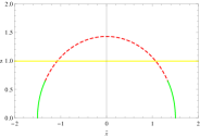
(a) $v_{*}=-0.856,\alpha=-0.1$

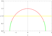
(b) $v_{*}=-0.856,\alpha=0.0001$

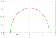
(c) $v_{*}=-0.856,\alpha=0.08$

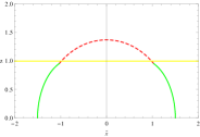
(d) $v_{*}=-0.456,\alpha=-0.1$

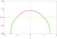
(e) $v_{*}=-0.456,\alpha=0.0001$

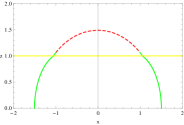
(f) $v_{*}=-0.456,\alpha=0.08$

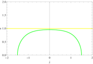
(g) $v_{*}=0.156,\alpha=-0.1$

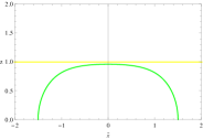
(h) $v_{*}=0.156,\alpha=0.0001$

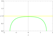
(i) $v_{*}=0.156,\alpha=0.08$

Figure 1: Motion profile of the geodesics in the Gauss-Bonnet Vaidya AdS black brane. The separation of the boundary field theory operator pair is $\tilde{\ell}=3$. The black brane horizon is indicated by the yellow line. The position of the shell is described by the junction between the dashed red line and the green line.

	$\alpha$=-0.1	$\alpha$=0.0001	$\alpha$=0.08
$v_{*}$=-0.856	0.691683	0.625454	0.560182
$v_{*}$=-0.456	1.01534	0.949695	0.888231
$v_{*}$=0.156	1.56525	1.50154	1.44083

Table 1: The thermalization time $t_{0}$ of the geodesic probe for different Gauss-Bonnet coefficient $\alpha$ and different initial time $v_{\star}$.

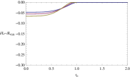
(a) $\tilde{l}=2$

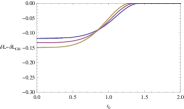
(b) $\tilde{l}=3$

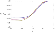
(c) $\tilde{l}=4$

Figure 2: Thermalization of the renormalized geodesic lengths in a Gauss-Bonnet Vaidya AdS black brane for different Gauss-Bonnet coefficients $\alpha$ and different boundary separations $\tilde{l}$. The green line, red line and purple line correspond to $\alpha=-0.1,0.0001,0.08$ respectively.

Figure (2) gives the relation between the renormalized geodesic length and thermalization time for different boundary separation that varies horizontally. In each picture, the vertical axis indicates the renormalized geodesic length while the horizontal axis indicates the time $t_{0}$. From the same color line, e.g. green line, in (a), (b) and (c) in Figure (2), we know that as the separation distance of local quantum field theory operators at the boundary increases, the thermalization time raises for a fixed Gauss-Bonnet coefficients $\alpha$. This result is consistent with that in [9, 10], which implies the UV thermalizes first. For a fixed separation distance, e.g. $\tilde{l}=2$, the thermalization time decreases as $\alpha$ becomes larger. This phenomenon has been also observed previously when we study the motion profile of the geodesic. In [11], the effect of charge on the thermalization time is investigated, it was shown that there is an enhancement of the thermalization time as the chemical potential over temperature ratio increases. Obviously, the Gauss-Bonnet coefficient has an opposite effect on the renormalized geodesic length compared with that case. In addition, in Figure (2), we observe that for a fixed boundary separation there is always a time range in which the renormalized geodesic length takes the same value nearly. That is, during that time range, the Gauss-Bonnet coefficient has little effect on the renormalized geodesic length.

Adopting similar strategy, we also can study the motion profile of minimal area and the relation between the renormalized minimal area surface and thermalization time. Based on the motion equations in (3.2) and the boundary conditions in (22), the numerical solution of $z(x)$ can be produced. In this case, we can get the motion profile of minimal area for different $\alpha$, which are shown in Figure (3). From this figure, we know that as the Gauss-Bonnet coefficient increases, the shell surface approaches to the horizon surface step by step. The thermalization time for different $\alpha$ have been listed in Table (2). It is obvious that the thermalization time decreases as $\alpha$ becomes larger. This behavior is similar to that of the geodesics. In addition, we also can substitute the numerical result of $z(x)$ into (30) to get the renormalized minimal area surface. Similar to the case of geodesic, we will plot $\delta A-\delta A_{GB}$, where $\delta A=\delta\tilde{A}/\tilde{l}$ and $\delta A_{GB}$ is the renormalized minimal area surface for a static Gauss-Bonnet AdS black brane. The relation between the renormalized minimal area surface and thermalization time is given in Figure (4), in which the vertical axis indicates the renormalized minimal area surface while the horizontal axis indicates the thermalization time $t_{0}$. We find that as the separation distance increases, the thermalization time raises for a fixed Gauss-Bonnet coefficient, which confirms the fact that the UV modes thermalize first. And for a fixed separation distance, the thermalization time decreases as $\alpha$ becomes larger. That is to say, the larger the Gauss-Bonnet coefficient is, the easier the quark gluon plasma thermalizes. This behavior is similar to that of the geodesic which is given in Figure (2). As the case of the renormalized geodesic length, we find that in Figure (4), there is also an overlapped region, where the Gauss-Bonnet coefficient has little effect on the renormalized minimal area surface.

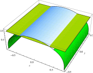
(a) $v_{*}=-0.252,\alpha=-0.1$

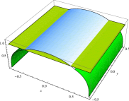
(b) $v_{*}=-0.252,\alpha=0.0001$

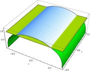
(c) $v_{*}=-0.252,\alpha=0.08$

Figure 3: Motion profile of the minimal area in the Gauss-Bonnet Vaidya AdS black brane. The boundary separation along the $x$ direction is $1.5$, and along the $y$ direction is $1$. The yellow surface is the location of the horizon. The position of the shell is is described by the junction between the white surface and the green surface.

	$\alpha$=-0.1	$\alpha$=0.0001	$\alpha$=0.08
$v_{*}$=-0.252	1.01732	0.963057	0.911427

Table 2: The thermalization time $t_{0}$ of the minimal area probe for different Gauss-Bonnet coefficients $\alpha$ with the same initial time $v_{\star}$.

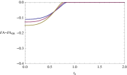
(a) $\tilde{l}=1$

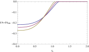
(b) $\tilde{l}=1.5$

(c) $\tilde{l}=2$

Figure 4: Thermalization of the renormalized minimal surface area in a Gauss-Bonnet Vaidya AdS black brane for different Gauss-Bonnet coefficients $\alpha$ and different boundary separations $\tilde{l}$. The green line, red line and purple line correspond to $\alpha=-0.1,0.0001,0.08$ respectively.

5 Conclusions

The thermalization time scale of the dual boundary field theory in Gauss-Bonnet gravity is studied in the framework of AdS/CFT correspondence. The thermalization process in the dual field theory is modeled by the collapsing of a shell of dust that interpolates between a pure AdS and a Gauss-Bonnet AdS black brane, in which the ground state is sufficiently excited by the injection of energy and followed by the thermalization. The two-point functions and expectation values of Wilson loops are chosen as the thermalization probes, which are dual to the renormalized geodesic length and minimal area surface in the bulk. The effect of the Gauss-Bonnet coefficients on the thermalization time is studied. We first obtain the motion profiles of the geodesic and minimal surface and find that for both cases the thermalization time decreases as the Gauss-Bonnet coefficient increases. We reproduce this result by studying the relation between the renormalized geodesic length and time as well as the renormalized minimal surface area and time respectively. In addition, for both the thermalization probes, we observe an overlapped region where the Gauss-Bonnet coefficient has few influence on them for a fixed boundary separation. The reason for this phenomenon maybe arises from the delay of the thermalization. As stressed in [10], the thermalization only becomes fully apparent at distances of the order of the thermal screening length $\tilde{l}_{D}\sim(\pi T)^{-1}$, where $T$ is the temperature of the dual conformal field. From (7), we know that the temperature is independent of the Gauss-Bonnet coefficient, so we can conclude safely that the thermalization for different $\alpha$ begins apparently at the almost same distance, leading to an overlap.

On the other hand, it is known from the viewpoint of holography that IIB string theory on AdS5 $\times S^{5}$ background is dual to $D=4,~{}N=4,~{}SU(N_{c})$ super Yang-Mills theory, and higher derivative corrections from string correspond to finite ’t Hooft coupling corrections. The most common corrections to the string are described by the terms $R^{4}$ and $R^{2}$ [34]. Recently Ref. [35] investigated the effect of $R^{4}$ corrections on the thermalization time scale in the framework of supergravity. They found that finite ’t Hooft coupling corrections decrease just a very little the thermalization time of UV modes, while they produce the opposite trend for IR modes. In this paper, we investigated one case of $R^{2}$ corrections, namely the Gauss-Bonnet gravity. We found that the Gauss-Bonnet coefficient will enhance the thermalization time for both the thermalization probes. It is also interesting to study the effect of $R^{2}$ corrections to the thermalization time scale in the framework of supergravity to compare with our work and that in [35].

References

- [1] D. Garfinkle and L. A. Pando Zayas, Rapid Thermalization in Field Theory from Gravitational Collapse, Phys. Rev. D 84, 066006 (2011) [arXiv:1106.2339 [hep-th]].
- [2] D. Garfinkle, L. A. Pando Zayas and D. Reichmann, on Field Theory Thermalization from Gravitational Collapse, JHEP 1202, 119 (2012) [arXiv:1110.5823 [hep-th]].
- [3] A. Allais and E. Tonni, holographic evolution of the mutual information, JHEP 1201 102 (2012) [arXiv:1110.1607 [hep-th]].
- [4] S. R. Das, Holographic Quantum Quench, J. Phys. Conf. Ser. 343, 012027 (2012) [arXiv:1111.7275 [hep-th]].
- [5] D. Steineder, S. A. Stricker and A. Vuorinen, probing the pattern of holographic thermalization with photons, arXiv:1304.3404 [hep-ph].
- [6] B. Wu, on holographic thermalization and gravitational collapse of massless scalar fields,JHEP 1210, 133 (2012)[arXiv:1208.1393 [hep-th]].
- [7] X. Gao, A. M. Garcia-Garcia, H. B. Zeng, H. Q. Zhang, Lack of thermalization in holographic superconductivity, arXiv:1212.1049 [hep-th].
- [8] W.J. Li, Y. Tian, H. Zhang, Periodically Driven Holographic Superconductor, arXiv:1305.1600 [hep-th].
- [9] V. Balasubramanian et al., Thermalization of Strongly Coupled Field Theories, Phys. Rev. Lett. 106, 191601 (2011) [arXiv:1012.4753 [hep-th]].
- [10] V. Balasubramanian et al., Holographic Thermalization, Phys. Rev. D 84, 026010 (2011) [arXiv:1103.2683 [hep-th]].
- [11] D. Galante and M. Schvellinger, Thermalization with a chemical potential from AdS spaces, JHEP 1207, 096 (2012) [arXiv:1205.1548 [hep-th]].
- [12] E. Caceres and A. Kundu, Holographic Thermalization with Chemical Potential, JHEP 1209, 055 (2012) [arXiv:1205.2354 [hep-th]].
- [13] W. H. Baron and M. Schvellinger, Quantum corrections to dynamical holographic thermalization: entanglement entropy and other non-local observables, arXiv:1305.2237 [hep-th].
- [14] W. Baron, Damian Galante and M. Schvellinger, Dynamics of holographic thermalization, arXiv:1212.5234 [hep-th].
- [15] I. Arefeva, A. Bagrov, A. S. Koshelev, Holographic Thermalization from Kerr-AdS, arXiv:1305.3267 [hep-th].
- [16] V. E. Hubeny, M. Rangamani, E.Tonni, Thermalization of Causal Holographic Information, arXiv:1302.0853 [hep-th].
- [17] V. Balasubramanian et al., Thermalization of the spectral function in strongly coupled two dimensional conformal field theories, arXiv:1212.6066 [hep-th].
- [18] I. Y. Arefeva, I. V. Volovich, On Holographic Thermalization and Dethermalization of Quark-Gluon Plasma, arXiv:1211.6041 [hep-th].
- [19] R. Gregory, S. Kanno and J. Soda, Holographic Superconductors with Higher Curvature Corrections, JHEP 0910, 010 (2009) [arXiv:0907.3203 [hep-th]].
- [20] Q. Pan et al., Holographic Superconductors with various condensates in Einstein-Gauss-Bonnet gravity, Phys. Rev. D 81, 106007 (2010) [arXiv:0912.2475 [hep-th]].
- [21] R. G. Cai, Z. Y. Nie and H. Q. Zhang, Holographic p-wave superconductors from Gauss- Bonnet gravity, Phys. Rev. D 82, 066007 (2010) [arXiv:1007.3321 [hep-th]].
- [22] J.P. Wu, Holographic fermions in charged Gauss-Bonnet black hole, JHEP 07, 106 (2011) [arXiv:1103.3982 [hep-th]].
- [23] Y. P.Hu, H.F. Li, Z.Y. Nie, The first order hydrodynamics via AdS/CFT correspondence in the Gauss-Bonnet gravity, JHEP, 1101, 123 (2011) [arXiv:1012.0174 [hep-th]].
- [24] D. Astefanesei, N. Banerjee, S. Dutta,(Un)attractor black holes in higher derivative AdS gravity, JHEP 0811, 070 (2008) [arXiv:0806.1334 [hep-th]].
- [25] R. G. Cai, Gauss-Bonnet black holes in AdS spaces, Phys. Rev. D 65, 084014 (2002) [arXiv:hep-th/0109133].
- [26] X. O. Camanho, J. D. Edelstein, Causality constraints in AdS/CFT from conformal collider physics and Gauss-Bonnet gravity, arXiv:0911.3160[hep-th].
- [27] X. O. Camanho, J. D. Edelstein, Causality in AdS/CFT and Lovelock theory, arXiv:0912.1944 [hep-th].
- [28] A. Buchel et al., Holographic GB gravity in arbitrary dimensions, JHEP 1003, 111 (2010) [arXiv:0911.4257 [hep-th]].
- [29] T. Kobayashi, A Vaidya-type radiating solution in Einstein-Gauss-Bonnet gravity and its application to braneworld, Gen. Rel. Grav. 37, 1869 (2005) [arXiv:gr-qc/0504027].
- [30] H. Maeda, Effects of Gauss-Bonnet term on the final fate of gravitational collapse, Class. Quant. Grav. 23, 2155(2006) [arXiv:gr-qc/0504028].
- [31] A. E. Dominguez, Emanuel Gallo, Radiating black hole solutions in Einstein-Gauss-Bonnet gravity, Phys.Rev. D 73, 064018 (2006) [arXiv:gr-qc/0512150].
- [32] V. Balasubramanian and S. F. Ross, Holographic particle detection, Phys. Rev. D 61, 044007 (2000) [arXiv:hep-th/9906226].
- [33] J. M. Maldacena, Wilson loops in large N field theories, Phys. Rev. Lett. 80, 4859 (1998) [arXiv:hep-th/9803002].
- [34] M. Ali-Akbari, K. Bitaghsir Fadafan, Conductivity at finite ’t Hooft coupling from AdS/CFT, arXiv:1008.2430 [hep-th].
- [35] W. H. Baron, M. Schvellinger, Quantum corrections to dynamical holographic thermalization: entanglement entropy and other non-local observables, arXiv:1305.2237 [hep-th].