From Josephson junction metamaterials to tunable pseudo-cavities

Abstract

The scattering through a Josephson junction interrupting a superconducting line is revisited including power leakage. We discuss also how to make tunable and broadband resonant mirrors by concatenating junctions. As an application, we show how to construct cavities using these mirrors, thus connecting two research fields: JJ quantum metamaterials and coupled cavity arrays. We finish by discussing the first non-linear corrections to the scattering and their measurable effects.

Keywords: Josephson junction, scattering, open transmission lines, superconducting cavities, metamaterials.

1 Introduction

Superconducting quantum circuits have demonstrated to be a flexible and scalable platform for quantum information processing  [1, 2]. Experimental proofs of simple quantum algorithms [3, 4], the first steps for many-body quantum simulations [5] and rapid improvements in the coherence times pave the way towards more scalable designs and experimental developments that beat what is classically computable or simulable. In addition to the quantum information route, quantum circuits are particularly interesting from a fundamental point of view, as a platform where both matter and light can be accurately engineered, with an unbeatable tunability, interaction strength [6, 7, 8] and scalability of designs.

While the experimental and theoretical focus was so far centered on the qubits, a new type of experiments and proposals are beginning to explore the study of propagating microwave photons and their interaction with artificial matter (qubits) or Josephson junctions. The building block of these studies is the scattering of photons through a qubit [9, 10, 11] or a Josephson junction (JJ) [12]. The reflection and transmission properties of these nonlinear scatterers have been probed in experiments with qubits [13, 14, 15] and SQUIDs [16]. More recently, arrangements of qubits or JJs have been suggested to tailor the propagation of light [17, 18, 19, 20, 12, 21], conforming what is now called quantum metamaterials, the topic of this special issue. These are low loss devices, since the underlying medium for the photon is a superconductor at a very low temperature, but they introduce new physics: from engineering of bandgaps and dispersion relation as in classical wave propagation, to purely quantum effects such as electromagnetic induced transparency (EIT) [22, 14] and other quantum phenomena.

There is an alternative paradigm for the study and control of light in quantum circuits and quantum optics: cavity-QED. Confining the light in optical cavities or resonators, the photon-qubit coupling can be enhanced (the Purcell effect) even to a point that the interaction energy gets close to the photon or qubit energy [6, 7]. Without resorting to this enhanced interaction regime, already at what is called the strong coupling, we find the possibility of engineering new quasiparticles, the polaritons, which are entangled states of light and matter [23, 24, 25]. These polaritons can be engineered in arrays of microwave cavities with embedded superconducting qubits [26, 27, 5], where the combined matter-light excitations move freely and implement sophisticated many-body Hamiltonians.

In this paper we merge both paradigms: that of quantum metamaterials and that of polaritonic arrays. The basic idea is that a Josephson junction may act as a mirror that reflects photons in a broad range of frequencies. We will show that embedding these junctions in a transmission line we can engineer localized modes that act as cavities with a moderate quality factor. This is similar to other designs where the pseudo-cavity is implemented by qubits [28], but we extend the idea from a single cavity, with two junctions, all the way to periodic arrangements of junctions that implement multiple coupled cavities. We discuss when this image is valid, what are the effective couplings between cavities and how these setups are related to our previous proposals on quantum metamaterials [12].

The paper is organized as follows. In the next section, Sect. 2, we review the single junction scattering. We include dissipation and a discussion on the power leakage. We complete the study with the reflection/transmission characteristics for concatenated junctions. In section 3 we apply the scattering theory for building cavities and relate the reflection and transmission of junctions with the coupling between different cavities. We continue by commenting on the first non linear corrections (Sect. 4) and the paper is finished with our conclusions.

2 Josephson junctions as scatterer

JJs are present in almost any superconducting quantum circuit, because they provide the non-linearity and the tunability which is needed in those circuits. In particular, they make it possible to build qubits and few-level systems [29], or tunable linear and non-linear resonators [30, 31, 32], and they are also used to shape and enhance the qubit-resonator coupling [6]. In addition, junctions are at the heart of recent works which introduce quantum metamaterials for shaping the transport of microwave photons [17, 18, 19, 20, 12, 16]. Working in the linear regime, the JJs act as local scatterers that can form band gaps and tailor the photon group velocity. Such setups may be generalized to two dimensions developing, e.g., left-hand metamaterials [12]. The main advantages of JJ-based quantum metamaterials are that they can be tuned (replacing the JJs by dc SQUIDs) and that their inherent losses are very small.

The minimal setup for observing the scattering of photons through a JJ consists on transmission line interrupted by a single junction, as sketched in Fig. 1(a). Constructing the equivalent lumped-element circuit from Fig. 1(b) and taking the continuum limit provides us with a Lagrangian that describes a transmission line with the junction [6, 32, 8, 12]

$$\mathcal{L} =\frac{1}{2}\int_{-\infty}^{0_{-}}{\rm d}x\left[c_{0}(\partial_{t}\phi)^{2}-\frac{1}{l_{0}}(\partial_{x}\phi)^{2}\right]$$

$$+\frac{1}{2}\left(\frac{\Phi_{0}}{2\pi}\right)^{2}C_{J}\left(\frac{d\varphi}{dt}\right)^{2}-\left(\frac{\Phi_{0}}{2\pi}\right)I_{C}\cos{\varphi}$$

$$+\frac{1}{2}\int_{0_{+}}^{\infty}{\rm d}x\left[c_{0}(\partial_{t}\phi)^{2}-\frac{1}{l_{0}}(\partial_{x}\phi)^{2}\right].$$

Through this work we assume that the capacitance and inductance per unit of length, $c_{0}$ and $l_{0}$ respectively, are constant along the line. The junction, placed at the origin, $x=0$, is characterized by a capacitance $C_{J}$ and a critical current $I_{C}$. While the microwave transmission line is described by a continuous field denoting the flux, $\phi(x,t)$, the Josephson junction has a unique degree of freedom associated to it, which is the gauge invariant phase, $\varphi$. This is given by

$$\varphi=\Delta\theta-\frac{2\pi}{\Phi_{0}}\int_{0_{-}}^{0_{+}}{\bf A}({\bf r},t)\cdot{\rm d}{\bf l}\;,$$ (2)

where $\Delta\theta$ is the superconducting phase difference and ${\bf A}({\bf r},t)$ is the vector potential. Note that since the junction is connected to two semi-infinite transmission lines, $\varphi$ is not be an independent variable, but depends on the incoming and outgoing fluxes

$$\varphi(t)\propto(\phi(0^{+},t)-\phi(0^{-},t)).$$ (3)

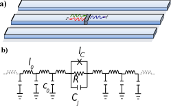
Figure 1: (color online) (a) An open transmission line interrupted by a Josephson junction (sketch). (b) Equivalent lumped element circuit, using the RCSJ model for the junction.

For studying the scattering of photons in the linear regime we must consider only perturbations of the equilibrium situation. We thus introduce the changes of the field, $\tilde{\phi}(x,t)$, with respect to the static background flux $\phi^{(0)}(x)$,

$$\phi(x,t)=\phi^{(0)}(x)+\tilde{\phi}(x,t).$$ (4)

We do the same for the junction, introducing a flux variable $\delta\phi(t)$ associated to the time fluctuations for the flux across the junction

$$\varphi(t)=\varphi^{(0)}+\frac{2\pi}{\Phi_{0}}\delta\phi(t)$$ (5)

Here $\varphi^{(0)}$ stands for the equilibrium solution for the phase and $V=(\Phi_{0}/2\pi)\dot{\varphi}=\dot{\delta\phi}$ is the expected voltage-flux relation.

Using the previous variables and the Lagrangian formalism we can construct equations for the propagation of photons through the junction [12]. We will complement those conservative differential equations with a model for the (possibly weak) losses on the junction itself. This is done in the lumped-element circuit model introducing the RCSJ model for the junction [33]: a resistance in parallel with the junction capacitance and the nonlinear inductance.

For the study of few-photon scattering, out of the resulting equations, we only need to consider the ones that match the fields to the right and to the left of the junction, through the Josephson relation. This is the equation of current conservation, which reads

$$\frac{1}{l_{0}}\partial_{x}\phi(0_{-},t)=\frac{\Phi_{0}}{2\pi}C_{J}\ddot{\varphi}+I_{C}\sin{\varphi}+\frac{1}{R}\frac{\Phi_{0}}{2\pi}\frac{d\varphi}{dt}=\frac{1}{l_{0}}\partial_{x}\phi(0_{+},t)$$ (6)

Since our studies focus on the low-power (few-photon) regime, we can linearize the equations, assuming small fluctuations in the junction phase, to obtain

$$\frac{1}{l_{0}}\partial_{x}\tilde{\phi}(0_{\pm},t)=C_{J}\,\ddot{\delta\phi}+\frac{1}{L_{J}}\,\delta\phi+\frac{1}{R}\dot{\delta\phi}$$ (7)

with $L_{J}=\Phi_{0}/(2\pi I_{C}\cos{(\varphi^{(0)})})$. Note that the linearization also provides us with the static configuration for the flux: $1/l_{0}\partial_{x}\phi^{(0)}(x)=I_{c}\sin(\varphi^{(0)})$.

In the linearized theory, the stationary scattering solutions can be written as a combination of incident, reflected and transmitted plane waves:

$$\tilde{\phi}(x,t)=A_{\phi}\left\{\begin{array}[]{cc}{\rm e}^{i(kx-\omega t)}+r{\rm e}^{-i(kx+\omega t)}&(x<0),\\ t{\rm e}^{i(kx-\omega t)}&(x>0),\end{array}\right.$$ (8)

where $A_{\phi}$ is the field amplitude, and $r$ and $t$ are the reflection and transmission coefficients, respectively. Outside the junctions the incoming and outgoing photons follow a linear dispersion relation, $\omega=vk$ with $v=1/\sqrt{l_{0}c_{0}}$, which we can substitute in the previous ansatz, to compute the transmission and reflection

$$r=\frac{1}{1-i2z\frac{1}{\bar{\omega}}\left(\bar{\omega}^{2}+i\gamma\bar{\omega}-1\right)},\quad t=1-r.$$ (9)

The scattering properties are a function of the photon frequency, $\bar{\omega}=\omega/\omega_{p}$, rescaled with the Josephson plasma frequency $\omega_{p}=1/\sqrt{L_{J}C_{J}}$. They also depend on the impedance of the line, $Z_{0}=\sqrt{l_{0}/c_{0}}$, and the junction, $Z_{J}=\sqrt{L_{J}/C_{J}}$, through their ratio $z=Z_{0}/Z_{J}$. Finally, dissipation enters via the dimensionless parameter $\gamma=Z_{J}/R$.

In the previous formulas we find a resonance at the plasma frequency of the junction, $\bar{\omega}=1$ or $\omega=\omega_{p}$. At this point the reflection becomes maximum and, in absence of dissipation, the junction behaves as a perfect mirror. A similar resonance mechanism is found when studying the scattering of photons through qubits  [9, 13]. This is illustrated in figure 2, where we plot the reflection-transmission characteristics, in the ideal (dashed) and dissipative (solid) cases. Note also that, as in classical wave propagation, the maximum of the reflection is accompanied by a phase jump of the scattered photon across the junction, as shown in figure 2b.

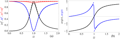
Figure 2: (color online) Transmission and reflection properties of a single junction acting as a scattering element. (a) Transmission, $t$, and reflection, $r$, for a junction without losses (dashed) and with losses ($\gamma=0.01$ or $R\sim 5\times 10^{3}\,\Omega$, solid), using $z=1.25$. We also plot the total outgoing photons, $|r|^{2}+|t|^{2}$, which close to resonance is less than 1 when in the presence of losses. (b) Phase of the transmitted and reflected photons, $arg(r)$ and $arg(t)$, respectively. Note the phase jump close to reflection, which is damped by the losses.

2.1 Power leakage

We already saw in Fig. 2(a) that for a dissipative junction the transmitted and reflected powers do not add up to one. Instead, some photons are absorbed by the junction and get lost, distorting slightly the resonance. It is instructive to have a closer look at the dissipation. For that we study the energy function in an interval of the line containing the junction:

$$E(x_{0})= \frac{1}{2}\int_{-x_{0}}^{0_{-}}{\rm d}x\left[c_{0}(\partial_{t}\phi)^{2}+\frac{1}{l_{0}}(\partial_{x}\phi)^{2}\right]$$

$$+\frac{1}{2}\left(\frac{\Phi_{0}}{2\pi}\right)^{2}C_{J}\left(\frac{d\varphi}{dt}\right)^{2}+\left(\frac{\Phi_{0}}{2\pi}\right)I_{C}\cos{\varphi}$$

$$+\frac{1}{2}\int_{0_{+}}^{x_{0}}{\rm d}x\left[c_{0}(\partial_{t}\phi)^{2}+\frac{1}{l_{0}}(\partial_{x}\phi)^{2}\right]\,.$$

Differentiating this functional with respect to time one obtains an expression that relates the dissipated power (loss of energy) to the flux drop around the junction

$$P=\frac{\partial E(x_{0})}{\partial t}=\frac{1}{l(x)}(\partial_{x}\phi)\dot{\phi}(x)|_{-x_{0}}^{x_{0}}.$$ (11)

Rather than the instantaneous power it is more illustrative to compute the average power in a cycle of the photon oscillations,

$$\bar{P}=\frac{\omega}{2\pi}\int_{0}^{2\pi/\omega}{\rm d}\tau P(\tau).$$ (12)

Combining the ansatz (8) together with the formulas for the transmission and reflection, $t$ and $r$ in Eq. (9), we get an expression that it is intuitively appealing

$$\bar{P}=A_{\phi}^{2}\frac{\omega^{2}}{2Z_{0}}\Big{(}1-|r|^{2}-|t|^{2}\Big{)}=2A_{\phi}^{2}\,Z_{0}\gamma\,\omega^{2}|r|^{2}$$ (13)

Roughly, the dissipated power is proportional to the incoming intensity and the reflected power, but also to the effective dissipation rate $\gamma$ of the junction. Dissipation is thus maximum only close to resonance, $|r|\sim 1$, where it degrades the reflection due to photon loss. Since the losses do not shift the resonance, which remains fixed at the condition $\bar{\omega}=1$, we obtain that the maximum dissipated power is

$$|r|^{2}_{(\bar{\omega}=1)}=\frac{1}{(1+2z\gamma)^{2}}\;\longrightarrow\bar{P}_{(\bar{\omega}=1)}=\frac{A_{\phi}^{2}}{Z_{0}}\frac{2z\gamma}{(1+2z\gamma)^{2}}.$$ (14)

Note that these results also apply to the context of microwave photodetection, where the loss mechanism is not the junction but an imperfect qubit. In this situation the maximum dissipated power can be directly related to the maximum detection efficiency [34].

2.2 JJs as tunable mirrors

While JJs may act as mirrors, it is well known that capacitors or cuts in the transmission line are higher quality mirrors. Why then study metamaterials constructed of JJs? There are several answers to this question. For starters, JJs offer the potential for nonlinear scattering of photons, discussed in Sect. 4. Most important, the reflectivity and transmission of a junction are frequency-dependent, acting as filters which suddenly become tunable when, instead of a junction, we use a dc SQUID. A dc SQUID is a circuit consisting on two junctions connected in parallel and threaded by some magnetic flux. The scattering properties of the dc SQUID are the same as those of a junction, but with the advantage that the plasma frequency, $\omega_{p}=1/\sqrt{L_{J}C_{J}}$, can now be tailored in situ via that external magnetic flux, $L_{J}=\Phi_{0}/[4\pi I_{C}\cos(\pi\Phi_{\rm ext}/\Phi_{0})]$, with $\Phi_{\rm ext}$ the external flux through the SQUID [Cf. Eq. (7)].

Another way in which the reflectivity of the junctions can be tuned is by combining several of them. As we will see below, this changes the bandwidth of the JJ filter, modifying the frequency-dependent transmission and reflection, and also the effect of losses —the mirror becomes more perfect. The idea of combining multiple scatterers to study their collective properties has been explored in the context of qubits, where two-level systems act as frequency-dependent mirrors [28]. Inspired by this work, we follow a similar route.

We will consider an arrangement of $N$ junctions disposed one after another separated by a distance $d$ in the same transmission line. If $d$ is large, we expect large oscillations of the scattering properties due to the constructive and destructive interference of the photons that are multiply reflected by the different junctions [34, 28]. Instead, we will focus on the limit in which the separation among junctions is so small, $d\ll\lambda$, that we can take the limit $d=0$ in the formulas. This is a very realistic assumption due to the difference in size —$d$ lays around the nanometer, while $\lambda$ is around the millimeter to centimeter. In this limit, we can neglect the phase acquired by the photons due to their propagation and regard the $N$ junctions in series through a generalization of Eq. (7) to $N+1$ equations of the form

$$\frac{1}{l_{0}}\partial_{x}\tilde{\phi}(0_{\pm},t)=C_{J}\,\ddot{\delta\phi}_{n}+\frac{1}{L_{J}}\,\delta\phi_{n}+\frac{1}{R}\dot{\delta\phi}_{n}\;\quad n=1,...,N$$ (15)

where $\delta\phi_{n}$ are the flux fluctuation across each junction. Assuming for simplicity that all junctions are identical, we obtain that the total flux fluctuation $\delta\phi=\tilde{\phi}(x_{+})-\tilde{\phi}(x_{-})$ is equally spread among junctions $\delta\phi_{n}=\delta\phi_{m}=\delta\phi/N$. In other words, the voltage drop along the circuit is equally divided among the junctions and the formula for the reflection gets then modified accordingly:

$$r=\frac{1}{1-i\frac{2z}{N}\frac{1}{\bar{\omega}}\left(\bar{\omega}^{2}+i\gamma\bar{\omega}-1\right)},\quad t=1-r.$$ (16)

The $N$ junctions behave as a single circuit, where transmission and reflection coefficients are modified by a factor $1/N$ in the denominator. The result is that, for a fixed ratio $Z_{J}/Z_{0}$ the number of concatenated junctions enlarge the resonance, as shown in Fig. 3.

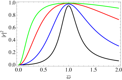
Figure 3: $|r|^{2}$ as a function of the number of junctions $N$. From bottom to top $N=1,2,4$ and 8 (colored as black, blue, red and green respectively). The rest of the parameters like in figure 2.

The concatenation of junctions also has a remarkable effect on the dissipation, increasing the quality factor of the mirror. Qualitatively, we expect that since the voltage drop is equally divided among the $N$, junctions, $\dot{\delta\phi}_{n}=\dot{\delta\phi}\sim r$, the losses at each junction should be decreased by the corresponding factor $1/N^{2}$. Summing over all $N$ junctions, the result should be that the dissipation scales as $1/N$, being reduced and increasing the quality of the overall circuit. Moreover, from Eq. (16) a reduction in the losses should be accompanied by an increase of the reflectivity. We can confirm this line of thought, combining all previous formulas for the reflection and the dissipated power

$$|r|^{2}_{\bar{\omega}=1}=\frac{1}{\left(1+\frac{2z}{N}\gamma\right)^{2}}\;\longrightarrow\bar{P}_{\bar{\omega}=1}=\frac{A_{\phi}^{2}}{Z_{0}}\frac{\frac{2z}{N}\gamma}{(1+\frac{2z}{N}\gamma)^{2}}$$ (17)

It would thus seem advantageous to use arrangements of multiple junctions or SQUIDs to build cavities, not only because the quality factor increases, but because the mirrors become broadband, allowing for a better definition of the localized mode. This is indeed the topic of the following section.

3 Pseudo-cavities

We have seen that Josephson junctions act as perfect mirrors for broad ranges of frequencies. It is natural then to wonder whether such mirrors can be used for building microwave cavities and what are their properties: quality factor, wavelengths, etc. We will show how these questions can be addressed using the scattering formalism developed above, studying the formation of one cavity, the coupling of two cavities and how these setups can be optimized and scaled up.

3.1 Localized mode for two junctions

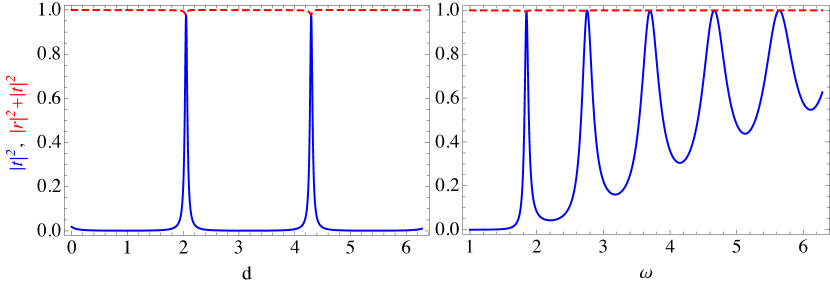
Figure 4: Transmission of a setup with two junctions separated a variable distance $d$ (blue line), and the sum of the transmission and reflection (dashed red line). Left: Resonances as a function of the separation between junctions, for $\omega=1.4$ and $z=0.2,\gamma=0.01$. Right: For a fixed cavity separation, $d=\pi$, different resonances associated to the fundamental and first harmonics of the pseudo-cavity.

Let us consider a photon propagating through a setup consisting on two junctions separated by a distance $d$. The transfer matrix of a single junction has a simple form in terms of the transmission and reflection coefficients

$$T=\left(\begin{array}[]{cc}1-\frac{r}{t}&\frac{r}{t}\\ -\frac{r}{t}&\frac{1}{t}\end{array}\right).$$ (18)

This matrix connects the left- and right-propagating components ($a$ and $b$ below) of a wave to one side and another side of the junction:

$$\left(\begin{array}[]{c}a_{L}\\ b_{L}\end{array}\right)=T\left(\begin{array}[]{c}a_{R}\\ b_{R}\end{array}\right).$$ (19)

For the ordinary propagation of a photon we have a similar transfer matrix, which only adds a phase to the fields

$$T_{prop}(d)=\left(\begin{array}[]{cc}e^{i\omega d/c}&0\\ 0&e^{-i\omega d/c}\end{array}\right),$$ (20)

where $c$ is the speed of the photons and $\omega$ the frequency. The whole transfer matrix of this cavity-like setup is

$$T_{2}=TT_{prop}(d)T,$$ (21)

which has an associated reflection coefficient

$$r_{2}\propto 2z(\omega^{2}+i\gamma\omega-1)\cos(d\omega/c)+\omega\sin(d\omega/c).$$ (22)

If we neglect the dissipation, the reflection has minima on a regular set of points, given by the equation

$$\tan(d\omega/c)=\frac{2z}{\omega}(1-\omega^{2}).$$ (23)

All the minima are spaced a distance $\pi c/\omega$, but their basic frequency is not exactly the wavelength of the photon, as shown in Fig. 4. Note also that for each separation between junctions, $d$, we also have a large number of resonances, corresponding to the bare resonance and the first harmonics. These additional modes are broader and have stronger decay rates, as it happens with similar setups where the mirrors are implemented using qubits instead of junctions [35]. In fact, for a sufficiently broadband mirror (assume $r={\rm const.}$ in the frequencies of interest) and high reflectivity, the quality factor is given by [36]

$$Q=\frac{\omega d}{2v_{g}(1-|r|^{2})}$$ (24)

with $v_{g}$ the group velocity in the line. Therefore and as expected, $Q$ increases with $N$. Note that the leakage in the cavity can be minimized by putting more junctions and it can be adjusted by detuning some of the junctions that act as a mirror.

3.2 Coupled cavities

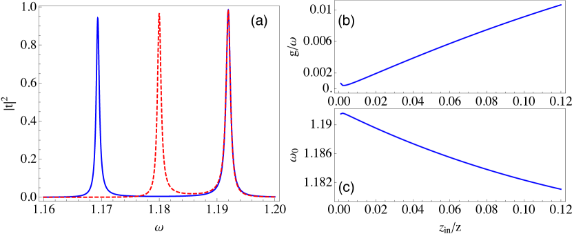
Figure 5: Transmission of a setup with two pseudo-cavities separated by an intermediate junction with parameter $z_{in}$. The cross-talk between the localized modes of both cavities produces two separated peaks in the transmission, whose separation is proportional to the coupling strength. (a) Resonances for $z_{in}=0.1$ (solid blue) and $z_{in}=0.05$ (dashed red). (b) Effective coupling strength as a function of $z_{in}/z$. (c) The central frequency between the peaks, $\omega_{0}$, shifts because of an interaction-induced renormalization. All simulations are computed assuming $\gamma=0.0001$, $d=2.6$ for the interjunction distance and using $z=0.1$ for the outer junctions.

To scale up the idea of implementing localized photons using junctions, we need to study the effective coupling between two such localized modes. For that we assume now a setup that consists on three junctions. The middle junction, characterized by $z_{in}$ [c.f. Eq. (9)], acts as a coupling element, while the outer junctions, characterized by $z$, separate the two cavities from the outer world. As before, we expect to have resonances at frequencies matching those of a system of coupled cavities, which we find studying the transmission and reflection properties of the combined setup.

In Fig. 5(a) we plot those properties for a setup with three junctions. We observe the appearance of two peaks around the central frequency $\omega\cong 1.18$. These two peaks account for the cavity-cavity coupling. As usual we estimate this effective coupling by using

$$\omega_{\pm}=\omega_{0}(g)\pm\frac{g}{2},$$ (25)

where the $g$ is the coupling strength and the middle frequency, $\omega_{0}$, may be slightly renormalized due also to the interactions. In Fig. 5(a) we plot the transmission for two different $z_{in}$, given different couplings and central frequencies.  A full dependence of the latter are shown in Figs. 5(b) and (c). In particular, in Fig. 5(b), we see that the interaction grows linearly with the ratio $z_{in}/z$. This was expected: decreasing $z_{in}$ implies increasing the reflectivity of the middle junction for this particular frequency, thus decoupling nearby photons. Finally, as the peak at the highest frequency remains fixed, the central frequency also moves to higher frequencies when the cavity-cavity coupling is enhanced as plotted in Fig. 5(c).

3.3 Arrays of cavities

The previous idea can be scaled up to construct arrays of coupled cavities. We simply have to use more junctions spaced regularly. The study of such systems becomes actually much simpler in the limit of infinite many junctions, when we focus on the solutions that preserve the number of photons, $\gamma=0$. In that case we can study the eigenstates of the problem assuming translational invariance, that is $\psi(x+d)=\psi(x)\exp(\pm ik)$, with $k$ the quasimomentum. As explained in Ref. [12], we have to solve the problem

$$2\cos(k)=\mathrm{tr}\left[T\,T_{prop}(d)\right],$$ (26)

which in our case reads

$$\cos(k)=\cos(d\omega)+\frac{\omega\sin(d\omega)}{2z(\omega^{2}+i\gamma\omega-1)},$$ (27)

where we will assume $\gamma=0$ for simplicity.

In our previous work [12] we focused on the creation of bandgaps and chose a junction separation, $d=0.3$, such that the photons were in the region with transmission close to one. In this work we are interested in recreating localized modes and thus $d$ must be a distance that resonates with the junction. Thus, the value of $d$ should be close to an integer multiple of $\pi$, producing plots such as the one in Fig. 6. In those plots we appreciate the existence of an infinite series of bands with a width, $\Delta\omega_{n}$, that grows with the frequency. We can regard these bands as the results of photons hopping between the pseudo-cavities. The central frequency of the $n$-th band would then correspond to the $n$-th harmonic of the pseudo-cavity [cf. Fig. 5], while the width of the cavity will be related to the cavity-cavity coupling, $g$, through the usual relation in a tight-binding model, $g=\frac{1}{2}\Delta\omega_{n}$.

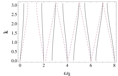
Figure 6: Eigenenergies $\omega_{k}$ vs. lattice quasimomentum $k$, for an array of junctions separated a distance $d=\pi$, with $z=0.1$ (solid) and $z=1$ (dashed) .

Naturally, the tight-binding approximation will work better when (i) the bands are mostly flat and (ii) the gap between consecutive bands remains large. This is, in turn, related to the properties of the junction that we use to build the cavities: the bandwidth decreases and the gap increases as we make $z$ smaller [cf. Fig. 6]. If we ensure the limit in which the localized-mode approximation remains valid, we can use this coupled-cavity array as a basis for the study of polariton physics [23, 24, 25], for instance, bridging the gap between the study of JJ quantum metamaterials and the quantum simulation of many-body physics.

4 Non-Linear corrections for the scattering

So far, we have assumed only linear dynamics for the junction. It behaved as a local impurity in the line with a resonance frequency $\omega_{p}$ and dissipation $\gamma$. In fact all the applications discussed were rooted in the linear approximation. On the other hand, the JJ is the paradigm of a nonlinear system, ranging from applications in classical dynamics: the circuit analogue for the pendulum, and in quantum physics: the artificial atom or qubit. Therefore it seems reasonable to check up to what extent the linear theory is accurate. Since we are interested in an estimation of the appearance of nonlinear corrections we fix our attention to the simplest situation, the scattering through a single junction neglecting dissipation.

For accounting to the nonlinear scattering we proceed as usual in nonlinear optics and perform an harmonic expansion for the left and right fields [37]:

$$\phi(x,t)=A_{\phi}\left\{\begin{array}[]{cc}{\rm Re}\left[{\rm e}^{-i(kx-\omega t)}+\sum_{n}r_{n}{\rm e}^{in(kx+\omega t)}\right]&(x<0)\\ {\rm Re}\left[\sum_{n}t_{n}{\rm e}^{-in(kx-\omega t)}\right]&(x>0)\end{array}\right.$$ (28)

We emphasize here that we must work with the real part from the beginning, since in the nonlinear case we will face with product between different harmonics. For the following it is convenient to split the reflection and transmission coefficients in real and imaginary parts $r_{n}=r_{n}^{\prime}+ir_{n}^{\prime\prime}$ and $t_{n}=t_{n}^{\prime}+it_{n}^{\prime\prime}$. We replace this ansatz in the equations for the current conservation (6). The equality of the current at both sides of the junction, $1/l_{0}\partial_{x}\tilde{\phi}(0_{-},t)=1/l_{0}\partial_{x}\tilde{\phi}(0_{+},t)$, implies

$$r_{n}^{\prime}+t_{n}^{\prime}=\delta_{n,1}\;\quad r_{n}^{\prime\prime}=t_{n}^{\prime\prime}\,.$$ (29)

Next, we match this current with current through the junction computed expanding the sine function up to the fifth order:

$$1/l_{0}\partial_{x}\tilde{\phi}(0_{-},t) = C_{J}\,\ddot{\delta\phi}+1/L_{j}\delta\phi$$

$$- 1/3!(2\pi)^{2}/\Phi_{0}^{2}L_{J}\delta\phi^{3}+1/5!(2\pi)^{4}/\Phi_{0}^{4}L_{J}\phi^{5}.$$

Then we merge this expansion with the one for the fields in Eq. (28) and match the different harmonics (fifth order).

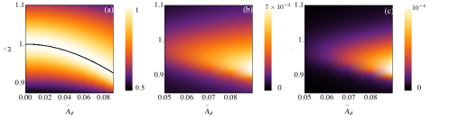
Figure 7: $|r_{1}|^{2}$, $|r_{3}|^{2}$ and $|r_{5}|^{2}$ as a function of the incoming amplitude $\bar{A}_{\phi}=A_{\phi}/\Phi_{0}$ and the normalized frequency $\bar{\omega}=\omega/\omega_{p}$. Black line is the theoretical prediction (4)

The numerical results are summarized in the figure 7. We notice that the nonlinear effects increase with the amplitude field $A_{\phi}$ and that they are present around $\omega_{p}$. We first plot $|r_{1}|$ (the reflected photons with the same frequency). The graphics show the expected shift in the resonance frequency $\omega_{p}$. The resonance frequency moves to lower frequencies. This is a consequence of the increase (decrease) of the pendulum period (frequency) as the amplitude increases. An analytical formula is available in textbooks:

$$T = \frac{4}{\omega_{J}}\int^{\pi/2}_{0}\frac{{\rm d}\theta}{\sqrt{1-(2\pi\bar{A}_{\phi})^{2}\sin(x)^{2}}}$$

$$\cong 2\pi\Big{(}1+\frac{1}{4}(2\pi\bar{A}_{\phi})^{2}+\frac{3}{4}(2\pi\bar{A}_{\phi})^{4}\Big{)}\,$$

where we have introduced $\bar{A}_{\phi}=A_{\phi}/\Phi_{0}$. This formula is plotted together with the numerical results, showing the agreement.

The other two plots stand for the $|r_{3}|$ and $|r_{5}|$, providing the third and fifth harmonic generation. These parameters, albeit small, are maximal whenever $|r|\cong 1$. To understand the latter, we remind that the current through the JJ depends on the flux difference $\delta\tilde{\phi}\sim t-r-1=-2r$ entering in the sine in (6), which is maximized at $|r|=1$. Here we have chosen the range of amplitudes $\bar{A}_{\phi}\leq 0.1$ which is the range where, in principle, the linear approximation is arguable. Notice that for expanding the sine function in Eq. (6), $2\pi/\Phi_{0}\delta\widetilde{\phi}\ll 1$ which implies $\bar{A}_{\phi}\ll 0.1$. To better quantify such a number, let us consider the case of a cavity build up with JJs as mirrors. Considering the quantization of the photons inside the cavity $\phi=\sqrt{\hbar Z}(a^{\dagger}+a)$ yields that $2n+1=\bar{A}_{\phi}^{2}\Phi_{0}^{2}/\hbar Z$. This reasoning implies that at amplitudes $\bar{A}_{\phi}=0.1$ the number of photons is around 4 (see also [39]). When considering the mirror formed by N junctions and recalling Sect. 2.2 the jump at each junction is spread among the junctions: $\delta\phi_{n}=\delta\phi/N$ [Cf. Eq. (15)]. Consequently the number of photons scale at the mentioned amplitude $\bar{A}_{\phi}=0.1$ as $4N^{2}$.

5 Conclusions and outlook

In summary, we have discussed the scattering characteristics of Josephson junctions when they are embedded in superconducting transmission lines. The JJs are resonant scatterers such that, whenever the incident photon matches the plasma frequency the junction behaves as a perfect mirror. Away from the resonance the junction is transparent. In this work we also included dissipative effects, which play a role near resonance by degrading the perfect reflection. Importantly enough the broadband, resonance frequency and even the dissipation can be tuned. This is the great advantage.

The frequency dependence of the scattering can be used as a building block for metamaterials, tailoring the photon propagation as discussed previously [12]. In this work, however, we have used this resonant character to propose the building up arrays of coupled quantum cavities [38]. Importantly enough the coupling may be tuned in situ via external fields. We show that it is possible to use coupled-cavity array as a basis for the study of polariton physics, for instance, bridging the gap between the study of JJ quantum metamaterials and the quantum simulation of many-body physics.

Finally we discussed the nonlinear corrections to the scattering. While the calculations are expected to be valid in the few photon limit we argue that the appearance of those nonlinear corrections can also be controlled by the number of junctions forming the mirrors. This can be used both for minimizing the nonlinear corrections or to favor them for achieving nonlinear cavity-cavity coupling [39]. The latter is important for the study of phases in Bose-Hubbard like models [40].

This work was supported by Spanish government projects FIS2009-10061, and FIS2011-25167 cofinanced by FEDER funds. We thanks Aragón government support to group FENOL, CAM research consortium QUITEMAD and PROMISCE European project.

References

References

- [1] You J Q and Nori F 2011 Nature 474 589-97
- [2] Buluta I, Ashhab S and Nori F 2011 Rep. Prog. Phys. 74 104401
- [3] Dicarlo L, Chow J M, Gambetta J M, Bishop L S, Johnson B R, Schuster D I, Majer J, Blais A, Frunzio L, Girvin S M and Schoelkopf R J 2009 Nature 460 240-4
- [4] Mariantoni M, Wang H, Yamamoto T, Neeley M, Bialczak R C, Chen Y, Lenander M, Lucero E, O’Connell A D, Sank D, Weides M, Wenner J, Yin Y, Zhao J, Korotkov A N, Cleland A N and Martinis J M 2011 Science 334 61-5
- [5] Houck A A, Türeci H E and Koch J 2012 Nature Physics 8 292-9
- [6] Niemczyk T, Deppe F, Huebl H, Menzel E P, Hocke F, Schwarz M J, García-Ripoll J J, Zueco D, Hummer T, Solano E, Marx A and Gross R 2010 Nature Physics 6 772-6
- [7] Forn-Díaz P, Lisenfeld J, Marcos D, García-Ripoll J J, Solano E, Harmans C J P M and Mooij J E 2010 Phys. Rev. Lett. 105 237001
- [8] Bourassa J, Gambetta J M, Abdumalikov A A, Astafiev O, Nakamura Y and Blais A 2009 Phys. Rev. A bf 80 032109
- [9] Shen J T and Fan S 2005 Phys. Rev. Lett. 95 213001
- [10] Zhou L, Gong Z, Liu Y, Sun C and Nori F 2008 Phys. Rev. Lett. 101 100501
- [11] Zhou L, Dong H, Liu Y, Sun C and Nori F 2008 Phys. Rev. A 78 063827
- [12] Zueco D, Mazo J J, Solano E and García-Ripoll J J 2012 Phys. Rev. B 86 024503
- [13] Astafiev O, Zagoskin A M, Abdumalikov A A, Pashkin Y, Yamamoto T, Inomata K, Nakamura Y and Tsai J S 2010 Science 327 840-3
- [14] Hoi I C, Wilson C M, Johansson G, Palomaki T, Peropadre B and Delsing P 2011 Phys. Rev. Lett. 107 073601
- [15] Astafiev O V, Abdumalikov A A, Zagoskin A M, Pashkin Y A, Nakamura Y and Tsai J S 2010 Phys. Rev. Lett. 104 183603
- [16] Jung P, Butz S, Shitov S V and Ustinov A V 2013 arXiv:1301.0440
- [17] Rakhmanov A L, Zagoskin A M, Savel’ev S and Nori F 2008 Phys. Rev. B 77 144507
- [18] Zagoskin A M, Rakhmanov A L, Savel’ev S and Nori F 2009 Phys. Stat. Solid (b) 246 955-960
- [19] Nation P D, Blencowe M P, Rimberg A J and Buks E 2009 Phys. Rev. Lett. 103 087004
- [20] Hutter C, Tholén E A, Stannigel K, Lidmar J and Haviland D B 2011 Phys. Rev. B 83 014511
- [21] Mukhin S I and Fistul M V 2013 arXiv:1302.5558
- [22] Abdumalikov A A, Astafiev O, Zagoskin A M, Pashkin Yu A, Nakamura Y and Tsai J S 2010 Phys. Rev. Lett. 104 193601
- [23] Hartmann M J, Brandão F G S L and Plenio M B 2006 Nature Physics 2 849-855
- [24] Greentree A D, Tahan C, Cole J H and Hollenberg Y C L 2006 Nature Physics 2 856-861
- [25] Angelakis D G, Santos M F and Bose S 2007 Phys. Rev. A 76 031805
- [26] Koch J and Le Hur K 2009 Physical Review A 80 023811
- [27] Hümmer T, Reuther G, Hänggi P and Zueco D 2012 Physical Review A 85 052320
- [28] Chang Y, Gong Z R and Sun C P 2011 Phys. Rev. A 83 013825
- [29] Makhlin Y, Schön G and Shnirman A 2001 Rev. Mod. Phys. 73 357-400
- [30] Castellanos-Beltran M A, Irwin K D, Hilton G C, Vale L R and Lehnert K W 2008 Nature Physics 4 929-931
- [31] Wilson C M, Johansson G, Pourkabirian A, Johansson J R, Duty T, Nori F and Delsing P 2011 Nature 479 376-9
- [32] Ong F R, Boissonneault M, Mallet F, Palacios-Laloy A, Dewes A, Doherty A C, Blais A, Bertet P, Vion D and Esteve D 2001 Phys. Rev. Lett. 106 167002
- [33] Orlando T P and Delin K A 1991 Foundations of Applied Superconductivity (Prentice Hall)
- [34] Romero G, García-Ripoll J J and Solano E 2009 Phys. Rev. Lett. 102 173602
- [35] Dong H, Gong Z R, Ian H, Zhou L and Sun C P 2009 Phys. Rev. A 79 063847
- [36] Hummer T, García-Vidal F J, Martín-Moreno L, Zueco D 2012 arXiv:1209.1724
- [37] Boyd R W 2003 Nonlinear Optics (Academic Press)
- [38] Liao J., Gong Z. R., Zhou L., Liu Y., Sun C. P. and Nori F. 2010 Phys. Rev. A 81 042304
- [39] Peropadre B, Zueco D, Wulschner F, Deppe F, Marx A, Gross R and García-Ripoll J J 2012 arXiv:1207.3408
- [40] Jin J, Rossini D, Fazio R, Leib M and Hartmann M J 2013 arXiv:1302.2242