The very energetic, broad-lined type Ic Supernova 2010ah (PTF10bzf) in the context of GRB/SNe

Abstract

SN 2010ah, a very broad-lined type Ic Supernova (SN) discovered by the Palomar Transient Factory, was interesting because of its relatively high luminosity and the high velocity of the absorption lines, which was comparable to that of Gamma-ray Burst (GRB)/SNe, suggesting a high explosion kinetic energy. However, no GRB was detected in association with the SN. Here, the properties of SN 2010ah are determined with higher accuracy than previous studies through modelling. New Subaru telescope photometry is presented. A bolometric light curve is constructed taking advantage of the spectral similarity with SN 1998bw. Radiation transport tools are used to reproduce the spectra and the light curve. The results thus obtained regarding ejecta mass, composition and kinetic energy are then used to compute a synthetic light curve. This is in reasonable agreement with the early bolometric light curve of SN 2010ah, but a high abundance of ⁵⁶Ni at high velocity is required to reproduce the early rise, while a dense inner core must be used to reproduce the slow decline at late phases. The high-velocity ⁵⁶Ni cannot have been located on our line of sight, which may be indirect evidence for an off-axis, aspherical explosion. The main properties of SN 2010ah are: ejected mass $M_{\rm ej}$ $\approx 3{\rm M}_{\odot}$; kinetic energy $E_{\rm kin}$  $\approx 10^{52}$ erg, M(⁵⁶Ni) $\approx 0.25{\rm M}_{\odot}$. The mass located at $v\mathrel{\hbox to0.0pt{\lower 4.0pt\hbox{\hskip 1.0pt$\sim$}\hss}\raise 1.0pt\hbox{$>$}}0.1$ c is $\sim 0.2{\rm M}_{\odot}$. Although these values, in particular the $E_{\rm kin}$, are quite large for a SN Ic, they are all smaller (especially $M_{\rm ej}$) than those typical of GRB/SNe. This confirms the tendency for these quantities to correlate, and suggests that there are minimum requirements for a GRB/SN, which SN 2010ah may not meet although it comes quite close. Depending on whether a neutron star or a black hole was formed following core collapse, SN 2010ah was the explosion of a CO core of $\sim 5-6{\rm M}_{\odot}$, pointing to a progenitor mass of $\sim 24-28{\rm M}_{\odot}$.

1 Introduction

Type Ib/c supernovae are perhaps the most diverse subtype of SNe. Their spectroscopic definition (no H (type Ib), no He (type Ic), weak Si, see Filippenko, 1997) means that this is the class in which almost all “strange” SNe are confined. SNe Ib/c include all explosions of massive stars that have lost their outer envelopes. The diversity of possible progenitors and evolutionary histories is reflected in the huge variety of properties of SNe Ib/c, which range from low (“normal”?) luminosity and kinetic energy (e.g. SN 1994I, Richmond et al., 1996; Iwamoto et al., 1994; Sauer et al., 2006) to broad-lined SNe Ic (e.g. SN 2002ap, Mazzali et al., 2002; Foley et al., 2003; Gal-Yam et al., 2002), to XRF-connected SNe Ib (e.g. SN 2008D, Soderberg et al., 2008; Mazzali et al., 2008; Modjaz et al., 2008) and SNe Ic (e.g. SN 2006aj, Pian et al., 2006), to luminous and energetic GRB/SNe Ic (SN 1998bw, Galama et al. (1998); SN 2003dh, Stanek et al. (2003); Hjorth et al. (2003); Matheson et al. (2003); SN 2003lw, Malesani et al. (2004)). The SN IIb subtype, where a small fraction of the H envelope survives, showing up in the spectrum but leaving practically no imprint on the light curve (Hachinger at al., 2012), also belongs to the same physical group. SNe IIb are also known to range from low (e.g. SN 1993J, Filippenko et al., 1993) to high energy events (e.g. SN 2003bg, Hamuy et al., 2009). Binarity is suspected to play a major role in the evolution of their progenitors (Nomoto et al., 1995; Maund et al., ; Crockett et al., 2008; Arcavi, 2011; Van Dyk et al., 2011; Maund et al., 2011). Some very bright SNe Ic are possibly linked to the pair instability phenomenon in very massive stars (e.g. the SN Ic 2007bi, Gal-Yam et al., 2009). Among the members of this class are also very luminous SNe whose origin is still debated (e.g. SN 2005ap, Quimby et al. (2007, 2011); Gal-Yam (2012), and references therein) or PS1-10afx, (Chornock et al., 2013). Finally, at the opposite end of the distribution, very dim SNe Ib such as 2005E and other “Ca-rich SNe” (Perets et al., 2010; Kasliwal et al., 2012) may be the result of the explosive ejection of a shell from the surface of a He-accreting white dwarf. All these SNe are also formally members of the SN Ib/c class, but their physical origin can be very different.

Still, the connection between SNe Ib/c, massive stars and GRBs is one of the most important reasons to study these stellar explosions. While extremely massive stars (M$\geq 80{\rm M}_{\odot}$) are believed to explode via the Pair Instability mechanism, which leaves no remnant, stars more massive than $\sim 25{\rm M}_{\odot}$ should collapse to form black holes. This mechanism is thought to be responsible for the emission of long-soft GRBs (Woosley, 1993). Although the details of the energy extraction are not yet understood, there is sufficient energy to power a relativistic jet (MacFadyen & Woosley, 1999; Bromberg, 2011). In fact, all well observed GRB/SNe are broad-lined SNe Ic, and all have been inferred to have large ejected mass and kinetic energy (Iwamoto et al., 1998; Mazzali et al., 2003, 2006b). These quantities are derived from modelling the light curves and spectra of these SNe, and the results consistently yield ejected masses of $\sim 10{\rm M}_{\odot}$, kinetic energies of several $10^{52}$ erg, ⁵⁶Ni masses of $\sim 0.5{\rm M}_{\odot}$, which have been used to infer progenitor star masses of $35-50{\rm M}_{\odot}$.

On the other hand, X-ray Flash/SNe like SN 2006aj seem to come from stars of lower mass ($\sim 20{\rm M}_{\odot}$), suggesting that energy injection from a magnetar is the mechanism which originated the XRF and energised the explosion (Mazzali et al., 2006a).

There are various cases of broad-lined SNe Ic whose properties are intermediate between those of GRB/SNe and those of XRF/SNe and are apparently not accompanied by a relativistic outflow (e.g. SN 1997ef (Mazzali, Iwamoto, & Nomoto, 2000); SN 1997dq (Mazzali et al., 2004); SN 2002ap (Mazzali et al., 2002)). This may suggest that some of the properties of these SNe were not sufficient for the generation of a GRB. Alternatively, they may all have off-axis GRBs, but this seems to be ruled out by radio observations (Soderberg et al., 2006). Studies of the emission line profiles in the late, nebular phase (Mazzali et al., 2004, 2007, 2010) do not suggest the off-axis option for most of these SNe, although they clearly do so for some of them (Mazzali et al., 2005; Tanaka et al., 2008). Spectropolarimetry, which is available only in very few cases, also suggests that SNe Ic are aspherical (e.g.  Kawabata et al., 2002, 2003; Gorosabel et al., 2006, 2010), and that more energetic SNe are more aspherical than lower-energy ones (Tanaka et al., 2012).

Clearly, in order to improve our understanding of these explosions, we need to extend the observed sample, cover a broader range of SN properties. A particularly interesting domain is SNe Ib/c with properties straddling those of GRB- and non-GRB/SNe. The presence of a high-energy transient is certainly one of the dimensions that determine SN Ib/c properties, although not the only one. One of the few SNe that falls in this category is SN 2010ah/PTF10bzf, a bright, broad-lined SN Ic without a GRB, for which extremely high velocities were inferred (Corsi et al., 2011). In this paper we model the spectra and light curve of SN 2010ah with our Montecarlo radiation transport codes and determine its properties. Our work is based on the data presented by Corsi et al. (2011), but we add very accurate photometry obtained with the Subaru Telescope.

The paper is organised as follows. In section 2 we recap the properties of SN 2010ah. In section 3 we present the new Subaru photometry. In section 4 we discuss how we use the spectral similarity to SN 1998bw to build a bolometric light curve for SN 2010ah given the lack of multicolour photometry. The light curve of SN 2010ah is then compared to those of other hypernovae (HN). In section 5 we briefly recap our modelling method and present spectral models for SN 2010ah. In Section 6 the synthetic light curves computed based on the spectral modelling results are presented and compared to the bolometric light curve of SN 2010ah. Finally, Section 7 contains a discussion and conclusions.

2 PTF10bzf = SN 2010ah: observational properties

The bright, broad-lined SN Ic SN 2010ah was discovered by the Palomar Transient Factory (PTF, Law et al., 2009; Rau et al., 2009) on 23 Feb 2010 in a galaxy at a redshift $z=0.0498$ (Corsi et al., 2011). It reached $r=18.3$ mag on 2 Mar 2010. At a distance modulus of $36.7$ mag, this corresponds to an absolute magnitude $M_{R}\approx-18.4$ mag. This makes SN 2010ah a luminous SN, but not a record-breaker. Data from the PTF follow-up were published in Corsi et al. (2011). The SN was classified as a Type Ic from spectra obtained at Gemini-N and Keck Obs, which show very broad lines. Velocities in excess of $0.1c$ were measured in Ca ii and Si ii lines (Corsi et al., 2011, fig. 5). In fact, absorption lines in SN 2010ah are among the broadest ever, rivalling with GRB/SNe such as 1998bw. Corsi et al. (2011) suggested that the SN is intermediate in spectral properties between the GRB/SN 1998bw (Patat et al., 2001) and the non-GRB SN 1997ef (Mazzali, Iwamoto, & Nomoto, 2000). Actually, SN 1998bw is the closest match, as can be seen from figs. 2 and 3 of Corsi et al. (2011). However, no X-ray counterpart was detected for SN 2010ah.

The striking spectral similarity to SN 1998bw and the lack of an associated $\gamma$- or X-ray counterpart make SN 2010ah an interesting event. The $R$-band luminosity was comparable to that of other broad-lined SNe Ic without a GRB, like SN 2003jd or SN 2009bb, for both of which an off-axis GRB has been suggested (Mazzali et al., 2005; Soderberg et al., 2010, respectively). However, SNe 2003jd and 2009bb resemble one another spectroscopically and look much more like the XRF/SN 2006aj (Pignata et al., 2011, figs. 11, 12) than SN 2010ah or SN 1998bw.

In Figure 1 we compare the two available spectra of SN 2010ah with the spectra of SNe 1998bw and 2002ap that look most similar based on an eye estimate of the available ones. The overall similarity is apparent: all three SNe show extreme line blending. In particular, Ca ii IR and O i 7774 Å are blended, which requires sufficient ejecta with $v\mathrel{\hbox to0.0pt{\lower 4.0pt\hbox{\hskip 1.0pt$\sim$}\hss}\raise 1.0pt\hbox{$>$}}0.1c$. In the blue, most pseudo-emission peaks (which actually correspond to regions of low line opacity where photons can escape) are obliterated because of line blocking by high-velocity material (Fe, Cr, Ti). This effect is more apparent in SN 1998bw than in either SN 2002ap or 2010ah, indicating a higher metal content at high velocity. On the other hand, SN 2010ah seems to have the highest line velocity of the three SNe (Corsi et al., 2011). This is shown in particular by the blueshift of the Si ii 6355 Å absorption in the 7 Mar spectrum, which has $v\approx 18000$ km s^-1. Considering that the epoch of the spectrum is at least 12 days after explosion (Corsi et al., 2011), this velocity is exceptionally high, and similar only to GRB/SNe (Pian et al., 2006; Bufano, 2012).

The spectra of SN 2010ah and SN 2002ap used for the comparison are closer to one another in time than those of SN 1998bw. Based on the epochs of the spectra it can be roughly estimated that the time evolution of SN 2010ah is faster than that of SN 1998bw by about a factor 1.3. In Section 4 we show how this is in fact confirmed by the evolution of the light curves.

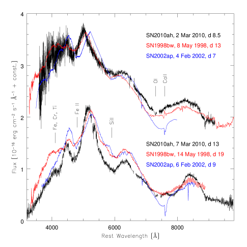
Figure 1: Comparison of the spectra of SNe 2010ah, 1998bw (Patat et al., 2001) and 2002ap (WHT service programmes) at similar epochs relative to the respective light curve evolution. Ions responsible for the strongest spectral features are marked.

3 New Subaru photometry and the light curves of SN 2010ah

The PTF follow-up campaign collected a good $r$-band light curve of SN 2010ah, but other bands were poorly sampled (Corsi et al., 2011). New Subaru data presented here improve the coverage in the post-maximum phase and make the calculation of a bolometric light curve more reliable.

Imaging observations of SN 2010ah in the $B$, $V$, and $R$-bands were performed under non-photometric conditions with the Subaru Telescope equipped with the Faint Object Camera and Spectrograph (FOCAS, Kashikawa et al., 2002) on 2010 Mar 19.25, 20.25, 21.25, and 22.24 UT (MJD = 55274.25, 55275.25, 55276.25, and 55277.24, respectively). The exposure time was 2 sec for each image. The images were bias-subtracted and flat-fielded. Photometry was performed relative to 5 stars in the field for the $R$ and $V$-band images and to 4 stars for the $B$-band images. We used an aperture of 1.5 times the full width at half-maximum (FWHM) of the point-spread function (PSF) of each image, estimated as the mean of the FWHM measured over the references stars and SN 2010ah. The magnitudes of the reference stars, originally in the SDSS system, were calibrated to $BVR$ using the conversions described in Jordi et al. (2006). Color corrections were applied to each image assuming that the measurement using the filter at the adjacent longer wavelength contains the information required to perform the correction. Zero-points and colour term coefficients were derived performing a linear fit on the reference stars for each image, and then used to derive the SN photometry for the corresponding image. The $B-V$, $V-R$, and $R-I$ colours of SN 2010ah were derived from WISE photometry (Corsi et al., 2011) at epochs close to those of the Subaru images. Since only 2 reference stars could be identified in the B-band image of Mar 19.25, the zero-point and colour term could not be determined, and a magnitude from this image could not be derived.

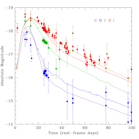
Figure 2: The UBVRI light curves of SN 2010ah. The light curves, dereddened with $E_{B-V}=0.012$, include the data presented in Corsi et al. (2011) and the new Subaru photometry (larger dots). The lines show the light curves of SN 1998bw, dereddened with $E_{B-V}=0.016$, dimmed by 0.5 mags and stretched in time by a factor $1.3^{-1}$. The light curves of SN 2010ah approximately match those of SN 1998bw.

Figure 2 shows the multiband photometry of SN 2010ah from Corsi et al. (2011) and the new Subaru data, highlighted as large circles. In order to build this figure, the photometric data originally acquired with filters different from the Johnson-Cousins system in the PTF campaign have been reduced to this system as follows. For the P48 data, $R=R_{Mould}-0.1$ was assumed. The P60 $griz$ magnitudes were transformed to $BRI$ using colours from simultaneous observations and normalisations as in Fukugita et al. (1996). Lacking spectroscopic information for SN 2010ah after maximum and based on the spectral similarity with SN 1998bw (see Figure 1), the $g,r,i,z$ and Mould-$R$ magnitudes of SN 2010ah have been converted to the $BVRI$ system and k-corrected following Hamuy et al. (1993) and Oke & Sandage (1968), using as templates the spectra of SN 1998bw at phases comparable to those of SN 2010ah, after application of a time-folding factor of 1.3. The UVOT U-band filters were transformed to $U$ magnitudes using the zero-points of Poole et al. (2008) and a $\lambda^{3}$ power-law for the UV spectrum. Finally, synthetic magnitudes were extracted from the Gemini and Keck spectra. As these were both taken with the slit positioned near the parallactic angle, we assumed that in both cases flux calibration is reasonable across the whole spectrum. When we measured the synthetic photometry we conservatively assigned an uncertainty of $\pm 0.3$ mag to both points, as in Corsi et al. (2011). The error on the first 2 $R$-band points has been increased to 0.2 mags because the k-correction for those points is based on extrapolation from a SN 1998bw spectrum whose epoch is 3.5 days later in the time frame of SN 2010ah. At early epochs the spectral shape may change significantly over this time interval.

A fiducial time of explosion was selected. Since the explosion date is constrained by an upper limit on 19 Feb 2010, 4 days before the first PTF detection (Corsi et al., 2011, fig. 2), we assumed that the explosion occurred 2 days before first detection.

In Fig. 2 all magnitudes have been dereddened with $E_{B-V}=0.012$ (Schlegel et al., 1998), adopting $R_{V}=3.1$ and the Galactic extinction curve of Cardelli et al. (1989). The comparison of the rest-frame light curves of SN 2010ah with the much better sampled ones of SN 1998bw in the same filters, and especially in the $R$-band, where SN 2010ah has been most intensively observed, confirms that the time evolution of SN 2010ah is faster than that of SN 1998bw by a factor of $\sim 1.3$. If the rest-frame monochromatic light curves of SN 1998bw are divided by this factor they match those of SN 2010ah reasonably well (Fig. 2), although bluer bands in SN 2010ah seem to evolve slightly faster than redder bands with respect to SN 1998bw. In the $U$-band, the two points available for SN 2010ah are below the SN 1998bw template, suggesting a more rapid decay in this band, and perhaps some modest local absorption.

4 SN 2010ah: the bolometric light curve

In order to build a successful model for SN 2010ah it is necessary to construct a bolometric light curve. This is essential for the estimate of the mass of ⁵⁶Ni synthesised in the explosion and as an input to our spectrum-synthesis code. Since PTF photometry was obtained almost exclusively in the $r$-band, it is difficult to construct a well sampled bolometric light curve. At the same time it would be dangerous to use $r$ as a proxy for bolometric because the bolometric correction from $r$ may be different from SN to SN.

In order to compute the bolometric light curve of SN 2010ah we made use of the spectroscopic similarity between SN 2010ah and SN 1998bw and of the similar temporal evolution after rescaling in time by a factor $1.3^{-1}$ (Figure 2, see also Deng et al., 2005). We therefore adopted for SN 2010ah the bolometric correction from $r$ obtained for SN 1998bw (Patat et al., 2001) at corresponding epochs (stretched in time by $1.3^{-1}$). The resulting bolometric light curve is shown in Fig. 3. The epoch and brightness of the peak are not very well determined, but the good coverage of the decline phase allows a model to be developed.

As a verification of this method, for the two epochs when spectra are available we integrated the flux under the spectra, added 20% to account for flux outside the optical range taking SN 1998bw as an example (e.g.  Melandri et al., 2012), and allowed for a conservatively large error to account for uncertain flux calibration of the spectra.

Also, again as a verification, a bolometric magnitude was computed directly from the monochromatic data when sufficient coverage of the spectrum was available. This includes the epochs of the Subaru photometry, when quasi-simultaneous WISE $I$-band data are also available (Corsi et al., 2011), and an epoch near 50 days, when $b,r$ and $i$ photometry is available. A correction of 20% was again added for flux outside the optical bands. These points are highlighted in Figures 3 and 4.

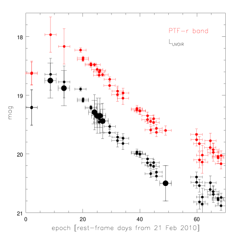
Figure 3: The PTF-r band light curve of SN 2010ah (red) and the bolometric light curve built from the photometry and correction with respect to SN 1998bw (black). Larger black points indicate estimates obtained directly from the spectra (near maximum) and from multi-colour photometry.

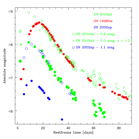
Figure 4: Comparison of bolometric light curves of different SNe Ic: Filled dots show the bolometric light curve of SN 2010ah, 1998bw and 2002ap. Empty green circles show the light curve of SN 2010ah shifted upwards by 0.9 mags. This is a good match to SN 1998bw in the declining phase. Green crosses show the light curve of SN 2010ah shifted upwards by 0.5 mags and stretched in time by a factor $(1.3)$. This is a good match to SN 1998bw except the earliest epochs. Empty blue dots show the light curve of SN 2002ap shifted upwards by 1.1 mags. This is a reasonable match to SN 2010ah.

4.1 SN properties derived from the light curve

A useful first step towards establishing a model for SN 2010ah is to derive basic information from the light curve and the spectra. In the spirit of Arnett (1982) this requires measuring the width of the light curve and a characteristic ejecta velocity from the spectra. These in turn can be transformed into first guesses for the ejected mass and kinetic energy. In Fig. 4 we compare the bolometric light curve of SNe 2010ah, 1998bw and 2002ap, all of which look similar spectroscopically. The light curve of SN 2010ah is very similar in shape to that of SN 2002ap, showing a fast rise to peak, which is reached within $\sim 10$ days. The light curve of SN 2010ah is $\sim 5$% broader than that of SN 2002ap, but significantly narrower ($\sim 25$%) than that of SN 1998bw. The characteristic velocity (at maximum) of SN 2010ah can be derived from fig. 5 of Corsi et al. (2011).

In order to obtain a rough estimate of the properties of SN 2010ah we can apply the well-known relations between ejected mass and velocity on the one hand and kinetic energy and light curve shape on the other (Arnett, 1982):

$$E_{\rm kin} \propto M_{\rm ej}v^{2}$$ (1)

$$\tau_{LC} \propto \frac{\kappa^{1/2}M_{\rm ej}^{3/4}}{E_{\rm kin}^{1/4}},$$ (2)

where $E_{\rm kin}$ is the kinetic energy of the ejecta, $M_{\rm ej}$ the ejected mass, $\kappa$ the optical opacity, $\tau_{LC}$ the characteristic width of the light curve. Adopting the commonly made assumption that $\kappa$ is constant in all SNe Ib/c, simple scaling relations can be obtained:

$$\frac{M_{1}}{M_{2}} \propto \left(\frac{\tau_{1}}{\tau_{2}}\right)^{2}\frac{v_{1}}{v_{2}}$$ (3)

$$\frac{E_{1}}{E_{2}} \propto \left(\frac{\tau_{1}}{\tau_{2}}\right)^{2}\left(\frac{v_{1}}{v_{2}}\right)^{3}$$ (4)

The results that are obtained from these relations depend sensitively on the choice of $v$. This is a characteristic ejecta velocity, and in itself it is not a very well defined quantity. Measuring line velocity and using that value has a number of shortcomings: 1) the velocity changes (decreases) with time; 2) the velocity at which lines form can be different (higher) than the momentary photosphere; 3) different lines may form at different velocities because of ionization or optical depth effects.

Adopting a velocity used for modelling (as for example was done for the SNe shown in fig.5 of Corsi et al. (2011), with the exception of SN 2010ah itself) eliminates at least some of these problems. Still, a single velocity does not represent the actual velocity distribution of the ejected matter. The velocity changes rapidly with time, and light curves have different shapes.

Very different results can be obtained if velocities at the same SN physical age (i.e. days from explosion, which is also an uncertain quantity except for GRB/SNe or for cases where shock breakout is detected) or at a particular phase of the light curve (e.g. maximum) are used, since different SNe peak at different physical times from explosion. Let us show some examples of this.

Since the epoch of maximum of the light curve of SN 2010ah is not well defined, different epochs can be chosen. Additionally, only two spectra are available. We use the velocity derived from the second spectrum (7 March 2010), 18000  km s^-1. Corsi et al. (2011) assigned to this spectrum an epoch of 11 days, based on the first detection. Corresponding velocities at this epoch can be obtained for both SN 1998bw (via interpolation) and SN 2002ap (from direct modelling). All values are shown in Table 1. The value of $E_{\rm kin}$ changes somewhat if we start from SN 1998bw or from SN 2002ap, reflecting the uncertainty in LC shape and time of maximum for SN 2010ah. Alternatively, we can consider the non-detection limit 4 days earlier, and assign to the March 7 spectrum a fiducial epoch of 13 days, as we do in the spectroscopic analysis below. The velocities of SNe 1998bw and 2002ap change significantly, despite the small change in epoch, and so do the results obtained for $M_{\rm ej}$ and $E_{\rm kin}$ of SN 2010ah. The value of $E_{\rm kin}$, in particular, is now much higher. Indicative results for SN 2010ah are $M_{\rm ej}$$\>\sim 4-6\>{\rm M}_{\odot}$, $E_{\rm kin}$$\>\sim(1.5-3)\>10^{52}$ erg, with large uncertainties. Similarly uncertain results would be obtained if we used the earlier spectrum as a reference for velocity. This shows that the rescaling method should be applied with caution, especially if the data coverage is not excellent. Furthermore, it is imperative that SNe are used that have very similar spectral properties in order to avoid carrying incorrect information (especially about $E_{\rm kin}$ as derived from velocities) from the SN used as template to the one which is being studied.

Table 1: Derived properties of SN 2010ah ($M_{\rm ej}$, $E_{\rm kin}$) with different assumptions about the epoch and using different reference SNe, whose $M_{\rm ej}$ and $E_{\rm kin}$ are given as are their velocities at different reference epochs.

SN	$\tau$	vel (11 d)	$M_{\rm ej}$	$E_{\rm kin}$
	days	km s-1	${\rm M}_{\odot}$	$10^{51}$ erg
1998bw	17	22500	10	50
2002ap	12	12000	2.5	4
2010ah	13	18000	5	15 (using 98bw)
	13	18000	4	15 (using 02ap)
SN	$\tau$	vel (13 d)	$M_{\rm ej}$	$E_{\rm kin}$
	days	km s-1	${\rm M}_{\odot}$	$10^{51}$ erg
1998bw	17	19000	10	50
2002ap	12	10000	2.5	4
2010ah	13	18000	6	25 (using 98bw)
	13	18000	5	25 (using 02ap)

The other important quantity that can be derived by interpolation is the mass of ⁵⁶Ni. This can be done using as reference the peak of the light curve, or alternatively the late phase. The use of different and independent methods makes the estimate of the M(⁵⁶Ni) more reliable than those of $M_{\rm ej}$ or $E_{\rm kin}$. Fig. 4 shows the two different approaches. The temporal evolution of the bolometric light curve of SN 2010ah looks rather similar to that of SN 2002ap. If the bolometric light curve of SN 2002ap is shifted up by 1.1 mag it tracks that of SN 2010ah very well, except for the first point, which suggests that SN 2010ah had a broader light curve. The early rise of the light curve of SN 2010ah may be due to mixing out of some ⁵⁶Ni, possibly in an aspherical explosion like that of SN 1998bw (Maeda et al., 2002, 2006). A shift of 1.1 mags corresponds to a factor 2.75 in luminosity. The mass of ⁵⁶Ni for SN 2002ap was determined from modelling as $0.07\>{\rm M}_{\odot}$ (Mazzali et al., 2002). This yields for SN 2010ah M(⁵⁶Ni$)\;=0.19\>{\rm M}_{\odot}$, consistent with the value derived by Corsi et al. (2011).

If we use as reference SN 1998bw, on the other hand, we can follow two different approaches. The post-maximum LC of SN 2010ah can be superposed on that of SN 1998bw if it is scaled up by 0.9 mags. This is a factor of 2.3 in luminosity. Adopting for SN 1998bw a ⁵⁶Ni mass of $0.41\>{\rm M}_{\odot}$ (Nakamura et al., 2001; Mazzali et al., 2006b), a ⁵⁶Ni mass of $0.19\>{\rm M}_{\odot}$ is obtained for SN 2010ah, consistent with the value obtained when rescaling from SN 2002ap. In fact, differences in the relative times are negligible at advanced epochs. This is therefore the safest approach.

Alternatively, one can rescale the bolometric light curve of SN 2010ah in flux AND stretch it by a factor 1.3 to generate a light curve that looks like that of SN 1998bw. In this case the rescaling factor is only 1.6 (0.5 mags), and the ⁵⁶Ni mass for SN 2010ah is $0.26\>{\rm M}_{\odot}$. This result is clearly inconsistent. The different time evolution of the two light curves must be taken into account: at early times the contribution of ⁵⁶Co can be ignored, and shifting the peak from 17 days (SN 1998bw) to 13 days (SN 2010ah) leads to a ⁵⁶Ni mass for SN 2010ah smaller by a factor of 0.63 with respect to the inital estimate. Hence we recover M(⁵⁶Ni)$=0.16{\rm M}_{\odot}$, which is reasonably consistent with the estimate based on the light curve tail. We conclude that for SN 2010ah M(⁵⁶Ni)$=0.18\pm 0.02{\rm M}_{\odot}$. A departure from this value can be introduced by a) any ⁵⁶Ni which is mixed to high velocities and is only visible in the rising phase; b) some deeply hidden ⁵⁶Ni which at peak does not yet contribute to the luminosity and only affects the light curve at very late times. This central ⁵⁶Ni is known to be present in a high density inner region in probably all hypernovae (Maeda et al., 2003). A signature of this deep ⁵⁶Ni may also be seen in SN 2010ah after about day 40, when the LC begins to flatten, although data unfortunately stop soon thereafter. Therefore, M(⁵⁶Ni)$=0.20{\rm M}_{\odot}$ is probably a lower limit for the mass of ⁵⁶Ni in SN 2010ah.

5 Spectral modelling

Given the description above, only accurate spectral (and light curve) modelling can yield reliable information on the properties of SNe Ib/c. For SN 2010ah only two spectra are available, so a very accurate result should not be expected. However, since the two spectra are separated by several days modelling may yield significant information.

We used our SN Montecarlo spectrum synthesis code, which was first presented by Mazzali & Lucy (1993). The code computes radiation transport in a SN ejecta starting from an assumed luminosity emitted at a lower boundary as a black body. SN ejecta are assumed to be in free expansion, so that $v=R/t$. Bound-free processes are ignored, but electron scattering and line absorption are considered. The latter is treated including the process of fluorescence, which is essential for the formation of type I SN spectra (Lucy, 1999; Mazzali, 2000). Radiative equilibrium is enforced in the SN envelope by conserving photon packets. Level populations are computed adopting a modified nebular approximation, which successfully accounts for the deviation from LTE. The code has been successfully applied to a number of different SNe Ib/c (e.g.  Mazzali et al., 2002), and it has proved a very useful tool to go beyond line identification: thanks to its physical treatment of opacities it allows different density and abundance profiles to be tested, so that various SN properties can be determined quantitatively.

Since our code uses a physical luminosity, flux-calibrated spectra are necessary for a meaningful comparison. The spectra are assumed to be reasonably well flux-calibrated based on the observational techniques used to obtain them. We corrected them for a Milky Way extinction of $E(B-V)=0.012$ (Schlegel et al. 1998) and measured R-band magnitudes using the PYSYNPHOT package. In order to account for calibration errors we applied a large error of 0.3 mags for both measurements. The corrected observed magnitudes are $R=17.95$ mag for the Gemini spectrum and $R=18.15$ mag for the Keck spectrum.

Our code requires as input a density distribution. This is essential in order to define the properties of the SN. In particular, SNe Ic with progressively broader lines are characterised by increasing values of the parameter $E_{\rm kin}$/$M_{\rm ej}$. Low-energy, “normal” SNe like SN 1994I have $E_{\rm kin}$/$M_{\rm ej}$$\sim 1$ (Sauer et al., 2006), while GRB/SNe like SN 1998bw, which show very broad lines, have $E_{\rm kin}$/$M_{\rm ej}$$>2$ (Nakamura et al., 2001). Given the spectral similarity between SN 2010ah, SN 1998bw and SN 2002ap, we adopt the explosion model that was used for SN 1998bw, rescaling it to match the parameters of SN 2010ah as estimated above.

We use a distance of 216 Mpc (i.e. a distance modulus $\mu=36.67$ mag) assuming $H_{0}=72$ km s^-1 Mpc^-1 and standard cosmology, and a reddening $E(B-V)=0.012$ (Corsi et al., 2011).

Given the estimated mass and energy of SN 2010ah, we started by rescaling the model for SN 1998bw (model CO138, $M_{\rm ej}$$=10{\rm M}_{\odot}$, $E_{\rm kin}$ $=3\>10^{52}$ erg, Iwamoto et al., 1998) by a factor between 0.3 and 0.5 in mass, which obviously implies a reduction in energy of the same magnitude.

Since both spectra are relatively early, our models can only probe the outer part of the ejecta. Therefore, while they can yield a reasonable estimate of the one-dimensional energy, which is mostly associated with the high-velocity outer ejecta, they cannot probe the bulk of the mass, which is located at lower velocities and deeper layers than the early spectra can reach. A more accurate estimate of the mass in this case requires modelling the light curve. Nebular spectra would be very useful for this purpose (e.g.  Mazzali et al., 2010), but none are available for SN 2010ah.

A fundamental element is the choice of risetime. The longer the risetime, the larger the ejected mass has to be in order to obtain a reasonable spectrum. SN 2010ah was first detected on 23.5 Feb 2010. The first spectrum was obtained on 2 Mar 2010, i.e.  7 days later. A deep non-detection limit 4 days prior to discovery means that the upper limit for the age of the first spectrum is 11 days (10.5 rest-frame days). Averaging these values, we assume $t=9$ days as the epoch of the first spectrum. Considering the redshift $(z=0.0498)$, we adopted for the 2 Mar spectrum $t=8.5$ d.

Our code computes a spectrum starting from the SN physical parameters $L,t$, and $v$, in order to define a consistent temperature structure in the ejecta. The photospheric velocity $v_{\rm ph}$ can be inferred from the spectra. Corsi et al. (2011) measured a Si ii 6355 Å absorption velocity $v=29000$ km s^-1 in the 2 March spectrum. We adopt for the model a slightly lower velocity, $25000$ km s^-1, and obtain a reasonable solution for the spectrum.

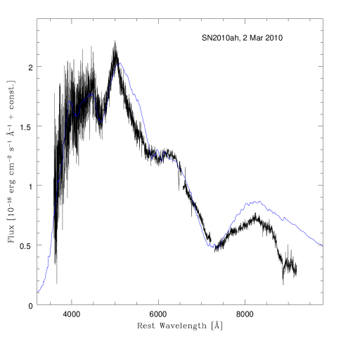
Figure 5: The spectrum of SN 2010ah obtained on 2 Mar 2010 (black) and the corresponding synthetic model (blue).

The luminosity necessary to reproduce the flux in the 2 Mar spectrum is $5\;10^{42}$ erg s^-1, i.e. $\log(L/L_{\odot})=9.12$. Given the rather small epoch, we find that the best results are obtained if model CO138 is rescaled in mass by a factor 0.3. This gives $M_{\rm ej}$$\,=3.2\>{\rm M}_{\odot}$; $E_{\rm kin}$$\;=10^{52}$ erg, but we should remark once more that the mass derived from the spectral fits alone can be highly uncertain since the spectra do not cover a large range of epochs. It appears however that a much smaller mass is located at high velocities than in the case of SN 1998bw, so we need to reduce the mass at $v>30000$ km s^-1. We did this by steepening the density slope, using a power-law $\rho(r)\propto r^{n}$ with index $n\approx-7$ above 20000 km s^-1. We find $\approx 0.2{\rm M}_{\odot}$ at $v>0.1c$, compared to $\approx 1{\rm M}_{\odot}$ for SN 1998bw. There is however practically no material at $v>10^{5}$ km s^-1, as was also the case for SN 1998bw. On 2 Mar 2010, only $\sim 0.5{\rm M}_{\odot}$ of material is found above $v_{\rm ph}$. The equivalent model for SN 1998bw had $\sim 1.2{\rm M}_{\odot}$ located above $v_{\rm ph}=31600$ km s^-1 on 3 May 1998 (Iwamoto et al., 1998), 8 days after explosion. Therefore the velocity of SN 2010ah is actually slightly smaller than that of SN 1998bw.

The synthetic spectrum is compared to the observed one in Fig. 5. Main features are Fe ii absorption at $\sim 4000$, 4600 Å, Si ii near 6000 Å, the O i-Ca ii blend near 7000 Å. The observed spectrum is reproduced adopting a composition above the photosphere dominated by oxygen (78% by number), followed by Ne (20%), intermediate-mass elements (5%). Ca and Fe are only present at the level of $\sim 0.5$%.

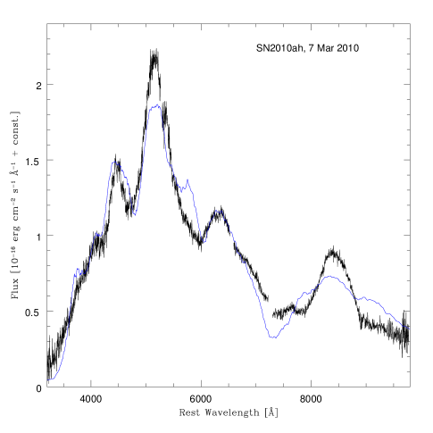
Figure 6: The spectrum of SN 2010ah obtained on 7 Mar 2010 (black) and the correspnding synthetic model (blue).

The next spectrum is only 5 days later, 7 Mar 2010. This corresponds to 14 days, (13.3 days in the rest frame). The velocity in this spectrum has dropped significantly (Corsi et al., 2011, measured 18000 km s^-1 in the Si ii  line), which is compatible with the drop observed in both GRB/HNe and non-GRB/HNe. We can thus probe deeper layers of the ejecta. The luminosity required to match the flux is $L=4\;10^{42}$ erg s^-1, i.e. $\log(L/L_{\odot})=9.01$. A velocity of $v_{\rm ph}=13500$ km s^-1 gives the best fit to the spectrum using the same density distribution as at the earlier epoch rescaled to the later epoch (Fig. 6). The photospheric velocity drops by much more than the observed Si ii velocity, suggesting that the observed feature is affected by other contributions. On the other hand, our synthetic Si ii line has a somewhat lower velocity than the observed one. At this epoch the mass above the photosphere is $2.25{\rm M}_{\odot}$. The composition is similar to that used for the previous epoch, with a little less oxygen (60%), replaced by neon (30%). The spectrum is still formed inside the oxygen layer. Abundances do not indicate enrichment of Intermediate-mass Elements or mixing-out of Fe. The synthetic O i line is too deep, but it is blended with Ca ii IR, which actually dominates in strength near 7500 Å. A lower density may lead to a better O i line, but the Si ii line would look worse. Since we only have these two spectra, we refrain from performing a more detailed but uncertain analysis. We rather turn to the light curve in order to determine parameters such as $M_{\rm ej}$, ⁵⁶Ni mass and distribution.

6 Light curve models

It is well known that light curve models alone do not have the ability to determine uniquely all SN parameters. In particular, while the mass of ⁵⁶Ni can be reasonably well established from the light curve peak if the time of explosion is known to within a good accuracy, or from the late, exponential decline phase of the light curve if this is observed, the two parameters that determine the shape of the light curve, $M_{\rm ej}$ and $E_{\rm kin}$, are degenerate (Eq.2; Arnett, 1982). Only the simultaneous use of light curve and spectra can break this degeneracy (Mazzali, Iwamoto, & Nomoto, 2000). Having established the most likely values of $M_{\rm ej}$ and $E_{\rm kin}$ through spectral modelling, we can test whether they can reproduce the light curve (Mazzali et al., 2002). Fitting the light curve yields additional information about the mass and distribution of ⁵⁶Ni, in particular at velocities lower than the photosphere sampled by the spectra. This is particularly useful for SN 2010ah, since for this SN we do not have nebular spectra, which would make it possible to obtain an accurate description of the inner ejecta (e.g.  Mazzali et al., 2010).

The properties of the light curve of a SN of Type I (i.e. H-free) are determined by the mass of ⁵⁶Ni, which determines the overall luminosity, and by the mass, density and composition of the ejecta. Mass and energy have a direct impact on the density of the ejecta as a function of time, and hence on the diffusion time of the photons. The abundances in the ejecta are important in that they determine the opacity (in a Type I SN this is dominated by line opacity; Pauldrach et al., 1996). If both early and late-time spectra are available, all these quantities can be independently determined through spectral modelling. Typically only small modifications to the mass and distribution of ⁵⁶Ni are required to reproduce the light curve and validate the results (Mazzali et al., 2009). This is however not the case for SN 2010ah, since no nebular spectra are available. Here we must rely on light curve modelling alone to establish the mass and density of the inner layers. Still, the properties of the outer layers are known from the early-time spectra, and so $E_{\rm kin}$ is reasonably well established.

We use the one-dimensional, monochromatic light curve code described in Cappellaro et al. (1997) and later modifications. The code is based on the Montecarlo method: given a density structure of the ejecta and a ⁵⁶Ni distribution, the emission and deposition of $\gamma$-rays and positrons produced in the radioactive decay of ⁵⁶Ni to ⁵⁶Co and hence to ⁵⁶Fe are computed. Deposition is assumed to be instantaneous, and to be followed by the emission of optical photons. Photon diffusion, which determines the light curve, is also followed with a Montecarlo scheme. Optical opacity is treated assuming that line opacity dominates: accordingly, it is assumed to depend on composition, as in Mazzali & Podsiadlowski (2006), reflecting the different number of active spectral lines in different atomic species.

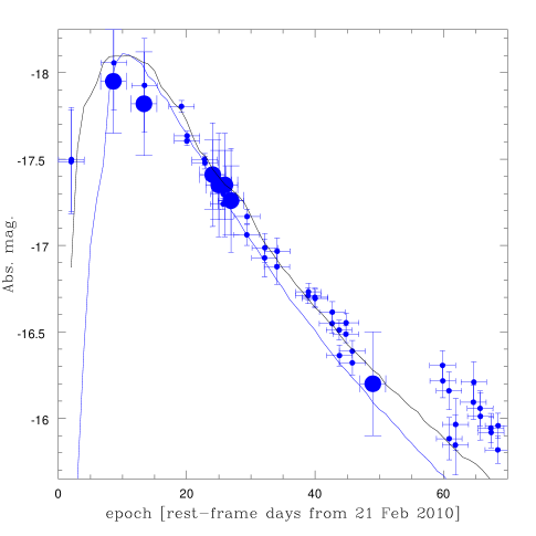
Figure 7: The $uvoir$ light curve of SN 2010ah and two models, one obtained using the rescaled explosion model used to fit the spectra (blue) and one where corrections have been applied for mixed-out ⁵⁶Ni and a dense inner core (black). The bigger blue points are those obtained from direct integration of the observed magnitudes from the spectra (near peak), from Subaru photometry ($\sim 25$ days), and at one late epoch (14 April 2010, 49 rest-frame days) when multiple photometry was available.

Initially, we use as input the density/abundance profiles derived from early-time spectral modelling. In particular, the model we used has $M_{\rm ej}$$=3.0{\rm M}_{\odot}$, $E_{\rm kin}$$=1.15\times 10^{52}$ erg. The result is the synthetic light curve shown in blue in Fig.7. This reproduces the maximum using a ⁵⁶Ni mass of $0.19{\rm M}_{\odot}$, but the rise is delayed relative to the observations. The decline is also well reproduced, but only until day 30 or so. Neither of these problems is new in the context of SN Ic light curve modelling: the slow rise of the synthetic light curve is typically the result of insufficient mixing-out of ⁵⁶Ni, while the slow observed late-time decline is actually common to all SNe Ic, and a solution was proposed that involves a dense low-velocity core, possibly a signature of an aspherical explosion (Maeda et al., 2003).

We therefore modified both the inner density and the outer ⁵⁶Ni abundance, and obtained the light curve shown in black in Fig. 7. This modified model has a power-law index $n\approx-1$ below 20000 km s^-1. It also has a slightly larger mass: $3.3\>{\rm M}_{\odot}$. The additional $0.2{\rm M}_{\odot}$ are located at $v<10000$ km s^-1. The ⁵⁶Ni distribution is also enhanced: outer layers ($v>20000$ km s^-1) contain a ⁵⁶Ni mass fraction of $\sim 10$%. This is much larger than the spectral modelling results, which indicate $\sim 1$%. The ⁵⁶Ni mass is now $0.25\>{\rm M}_{\odot}$ (instead of $0.19{\rm M}_{\odot}$), but because of the location of the additional ⁵⁶Ni there is no effect on the peak of the light curve, only on the rising phase. The highest ⁵⁶Ni abundance is at the lowest velocities, $v<3000$ km s^-1, where a mass fraction of more than 50% is reached. However, most of the ⁵⁶Ni is located at intermediate velocities, with a mass fraction of $\sim 15$% at 5000-10000 km s^-1 and $\sim 1$% at 10000-20000 km s^-1. The kinetic energy, on the other hand, is only marginally increased (now $1.19\>10^{52}$ erg instead of $1.15\>10^{52}$ erg). The modified model gives a better match to the overall light curve of SN 2010ah. Only the last phase ($t>60$ d) shows a discrepancy. A further increase in mass at very low velocities may be a solution, but we refrain from attempting such models because of the lack of later points to confirm the slower decline. Additionally, although galaxy subtraction has been applied homogeneously to all images (Corsi et al., 2011), since the galaxy brightness in $r$ is comparable to that of SN 2010ah at about 30 days after explosion, the presence of some residual at epochs $\mathrel{\hbox to0.0pt{\lower 4.0pt\hbox{\hskip 1.0pt$\sim$}\hss}\raise 1.0pt\hbox{$>$}}60$ days cannot be excluded. This may explain the excess seen in Fig. 7.

In the modified models ⁵⁶Ni is added mostly at high velocity ($>20000$ km s^-1). This requires reaching a ⁵⁶Ni mass fraction of $\sim 0.1$ in the outer ejecta. Although the ⁵⁶Ni distribution we have used yields a reasonably good match to the peak of the light curve of SN 2010ah, it is inconsistent with the abundance of ⁵⁶Ni and decay products required for the spectra. This discrepancy is potentially interesting. It may indicate that some ⁵⁶Ni was ejected at high velocity but not along our line of sight, so that it caused the rapid rise of the light curve (Maeda et al., 2006) without leaving an imprint on the spectra in the form of absorption lines.

Although this suggestion depends mostly on the first light curve point, this interpretation is appealing in view of the properties of highly energetic SNe Ic. We know from nebular spectroscopy that the distribution of elements is not spherically symmetric, in the sense that some ⁵⁶Ni and Fe are found at high velocities, probably in a funnel-like distribution which may track the position of the GRB jet in some cases (Mazzali et al., 2001), while oxygen and other unburned elements are ejected more in a plane, likely the equator of the progenitor. Two-dimensional models suggest this (Maeda et al., 2002). There is further evidence for asphericity in SNe Ib/c. Nebular studies suggest that even lower-energy SNe can be aspherical, albeit to a lesser degree (Maeda et al., 2008; Taubenberger et al., 2009; Modjaz et al., 2008; Maurer et al., 2010). It is also particularly interesting that in a SN Ib linked to an X-ray Flash (SN 2008D, Soderberg et al., 2008) spectral analysis suggests a high kinetic energy and the presence of a jet which was quenched by the helium shell (Mazzali et al., 2008), and later data confirmed asphericity in the oxygen distribution (Tanaka et al., 2008).

The kinetic energy derived for SN 2010ah is larger than that of SN 2008D, although smaller than in GRB/SNe, and the ejected mass is compatible with that of SN 2008D if the He shell in the latter is not considered. An off-axis, jet-driven SN was proposed for SN 2008D (Mazzali et al., 2008). More energetic SNe Ic are all linked to GRBs and aspherical (e.g.  Mazzali et al., 2001). Given the peculiarly high first point in the light curve of SN 2010ah, an aspherical distribution of elements may also be speculated for SN 2010ah. The lack of nebular or spectropolarimetric data prevents us from testing this hypothesis.

7 Discussion

The results of the analysis we performed can be used to estimate the properties of the progenitor of SN 2010ah. This is interesting, because of the suggested relation between $E_{\rm kin}$, M(⁵⁶Ni), and $M_{\rm ej}$, which should be a good proxy for the mass of the progenitor star (Mazzali et al., 2009). In the case of SN 2010ah, we found $M_{\rm ej}$$\,\sim 3.3\;{\rm M}_{\odot}$, $E_{\rm kin}$ $\sim 1.2\;10^{52}$ erg (in spherical symmetry), M(⁵⁶Ni)$\sim 0.25{\rm M}_{\odot}$.

If we plot the properties of SN 2010ah and those of other well studied SNe (Figures 8 and 9), we see a trend between $M_{\rm ej}$, M(⁵⁶Ni), and $E_{\rm kin}$. Figure 8 shows M(⁵⁶Ni) v. $E_{\rm kin}$. The trend is clear, although SN 2006aj deviates somewhat. In this case the birth of a magnetar was suggested (Mazzali et al., 2006a), and the energy released may have led to an increased synthesis of ⁵⁶Ni. Slightly more massive progenitors probably collapsed to a black hole, thus reducing the amount of material available for nucleosynthesis. At larger masses (and larger energies) the efficiency of production and ejection of ⁵⁶Ni increases again. Figure 9 shows M(⁵⁶Ni) v. $E_{\rm kin}$. Here the relation is less well defined, but a trend is still visible. SNe Ib and IIb have a massive He envelope and lie slightly higher in the plot, suggesting that the $E_{\rm kin}$ is not influenced by the properties of the outer layers, as is reasonable to expect.

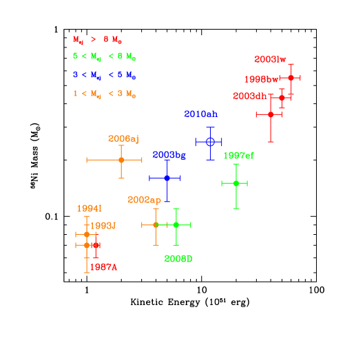
Figure 8: The mass of ⁵⁶Ni and the $E_{\rm kin}$ as derived from spectral/light curve modelling of a number of SNe Ib/c. Colour-coding is by ejected mass.

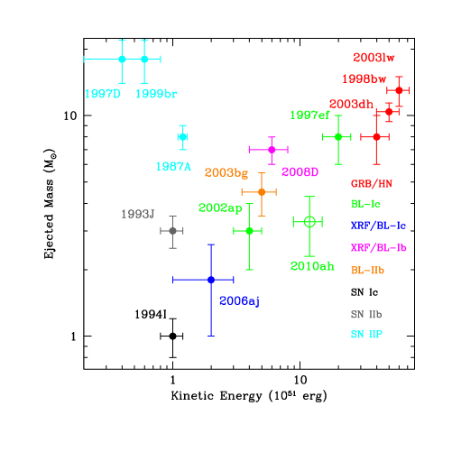
Figure 9: The ejecta mass and the $E_{\rm kin}$ derived from spectral/light curve modelling of a number of SNe Ib/c and some SNe IIP. Colour-coding is by spectral type.

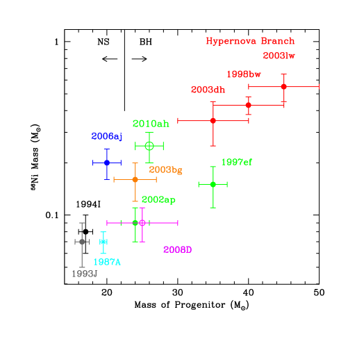
Figure 10: The mass of ⁵⁶Ni derived from spectral/light curve modelling of a number of SNe Ib/c plotted against the inferred ZAMS mass of the progenitor star using single-star evolutionary models. Colour-coding is by spectral type, and it is the same as in Fig. 9.

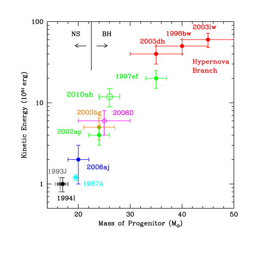
Figure 11: The $E_{\rm kin}$ derived from spectral/light curve modelling of a number of SNe Ib/c plotted against the inferred ZAMS mass of the progenitor star using single-star evolutionary models. Colour-coding is by spectral type, and it is the same as in Fig. 9.

We can try to go from the estimated $M_{\rm ej}$ to a progenitor mass. Using the Nomoto & Hashimoto (1988) models, and assuming that the mass ejected by SN 2010ah corresponds to the CO core of a massive star minus the remnant mass, we end up with a black hole remnant, a CO core of $\sim 5-6{\rm M}_{\odot}$, and a M${}_{ZAMS}\sim 24-28{\rm M}_{\odot}$. In the more traditional plots of M(⁵⁶Ni) or $E_{\rm kin}$ v. M_ZAMS (Figures 10 and 11), SN 2010ah falls nicely on the relation that is taking shape (e.g. Mazzali et al., 2009). This relation is derived for single-star evolution, and using a single, albeit old set of stellar models. The process of stripping the outer H and He layers may require interaction with a companion in a binary system (Fryer et al., 2007) and may not be easy to parametrise. Also, the uncertainty on the nature of the remnant (a Neutron Star or a Black Hole?) may introduce errors in the mass estimate.

Still, in the case of SN 2010ah, it looks as if all properties we derived ($M_{\rm ej}$, $E_{\rm kin}$, M(⁵⁶Ni)) are consistently smaller than those of GRB/SNe, although they are large compared to other non-GRB/HNe. We may be testing the limits for stars to produce GRBs. Another recent non-GRB/HN, SN 2010ay (Sanders et al., 2012) may come even closer to this limit and it will be an interesting case study.

A question remains concerning SN 2010ah: did it produce a GRB, or was it at least driven by a jet which failed to escape from the star, as was suggested for SN 2008D (Mazzali et al., 2008)? No detection of a GRB has been reported. Off-axis GRBs may be detected in the radio, but this is not the case for SN 2010ah (Corsi et al., 2011). The anomalously rapid rise of the light curve may suggest the presence of highly processed material in a direction not along our line of sight, but this cannot be regarded as a strong argument in the absence of other supporting evidence. Spectropolarimetry in the early phase or late-time spectroscopy would be useful in order to reveal asphericities. These may in turn point to the presence of a jet which, as in the case of SN 2008D (Tanaka et al., 2008), may have aided exploding the star even though it may not have emerged from it. Unfortunately, no such data are available for SN 2010ah, so we cannot determine the degree of asphericity or the presence of any asymmetry. A suggestion for asphericity drawn from the rapid rise of the light curve may be a point in favour of this. It would be important that exceptional SNe like SN 2010ah are studied in more detail in the future.

References

- Arcavi (2011) Arcavi, I. et al. 2011, ApJL, 742, L18
- Arnett (1982) Arnett, W. D. 1982, ApJ, 253, 785
- Bromberg (2011) Bromberg, O., Nakar, E., Piran, T., & Sari, R. 2011, ApJ, 740, 100
- Bufano (2012) Bufano, M., et al. 2012, ApJ753, 67
- Cappellaro et al. (1997) Cappellaro, E., et al. 1997, A&A, 328, 203
- Cardelli et al. (1989) Cardelli, J. A., Clayton, G. C., & Mathis, J. S. 1989, ApJ, 345, 245
- Chornock et al. (2013) Chornock, R., et al. 2013, arXiv:1302.0009
- Corsi et al. (2011) Corsi, A., et al. 2011, ApJ, 741, 76
- Crockett et al. (2008) Crockett, R. M., et al. 2008, MNRAS, 391, L5
- Deng et al. (2005) Deng, J., Tominaga, N., Mazzali, P. A., Maeda, K., & Nomoto, K. 2005, ApJ, 624, 898
- Filippenko et al. (1993) Filippenko, A. V., Matheson, T., & Ho, L. C. 1993, ApJL, 415, L103
- Filippenko (1997) Filippenko, A.V. 1997, ARAA, 35, 309
- Fryer et al. (2007) Fryer, C.L., et al. 2007, PASP, 119, 1211
- Foley et al. (2003) Foley, R. J., et al. 2003, PASP, 115, 1220
- Fukugita et al. (1996) Fukugita, M., Ichikawa, T., Gunn, J. E., Doi, M., Shimasaku, K., & Schneider, D. P. 1996, AJ, 111, 1748
- Galama et al. (1998) Galama, T.J., et al. 1998, Nat, 395, 670
- Gal-Yam et al. (2002) Gal-Yam, A., Ofek, E. O., & Shemmer, O. 2002, MNRAS, 332, L73
- Gal-Yam (2012) Gal-Yam, A. 2012, Science, 337, 927
- Gal-Yam et al. (2009) Gal-Yam, A., et al. 2009, Nat, 462, 624
- Gorosabel et al. (2006) Gorosabel, J., et al. 2006, A&A, 459, L33
- Gorosabel et al. (2010) Gorosabel, J., et al. 2010, A&A, 522, A14
- Hachinger at al. (2012) Hachinger, S., Mazzali, P. A., Taubenberger, S., Hillebrandt, W., Nomoto, K., & Sauer, D. N. 2012, MNRAS, 422, 70
- Hamuy et al. (1993) Hamuy, M., Phillips, M.M., Wells, L.A., & Maza, J. 1993, PASP, 105, 787
- Hamuy et al. (2009) Hamuy, M., et al. 2009, ApJ, 703, 1612
- Hjorth et al. (2003) Hjorth, J., et al. 2003, Nat, 423, 847
- Iwamoto et al. (1994) Iwamoto, K., et al. 1994, ApJL, 437, L115
- Iwamoto et al. (1998) Iwamoto, K., et al. 1998, Nat, 395, 672
- Jordi et al. (2006) Jordi, K., Grebel, E. K., & Ammon, K. 2006, A&A, 460, 339
- Kawabata et al. (2002) Kawabata, K. S., et al. 2002, ApJL, 580, L39
- Kawabata et al. (2003) Kawabata, K. S., et al. 2003, ApJL, 593, L19
- Kashikawa et al. (2002) Kashikawa, N., et al. 2002, Pub. Astron. Soc. Jap., 54, 819
- Kasliwal et al. (2012) Kasliwal, M., et al., 2012, ApJ, 755, 161
- Law et al. (2009) Law, N. M., et al. 2009, PASP, 121, 1395
- Lucy (1999) Lucy, L.B. 1999, A&A, 345, 211
- MacFadyen & Woosley (1999) MacFadyen, A. I., & Woosley, S. E. 1999, ApJ, 524, 262
- Maeda et al. (2002) Maeda, K., Nakamura, T., Nomoto, K., Mazzali, P. A., Patat, F., & Hachisu, I. 2002, ApJ, 565, 405
- Maeda et al. (2003) Maeda, K., Mazzali, P.A., Deng, J., Nomoto, K., Yoshii, Y., Tomita, H., & Kobayashi, Y. 2003, ApJ, 593, 931
- Maeda et al. (2006) Maeda, K., Mazzali, P. A., & Nomoto, K. 2006, ApJ, 645, 1331
- Maeda et al. (2008) Maeda, K., et al. 2008, Science, 319, 1220
- Malesani et al. (2004) Malesani, D., et al. 2004, ApJL, 609, L5
- Matheson et al. (2003) Matheson, T., et al. 2003, ApJ, 599, 394
- (42) Maund, J. R., Smartt, S. J., Kudritzki, R. P., Podsiadlowski, P., & Gilmore, G. F. 2004, Nat, 427, 129 ,
- Maund et al. (2011) Maund, J., et al. 2011, ApJL, 739, L37
- Maurer et al. (2010) Maurer, J. I., et al. 2010, MNRAS402, 161
- Mazzali (2000) Mazzali, P.A. 2000, A&A, 363, 705
- Mazzali & Lucy (1993) Mazzali, P.A., & Lucy, L.B. 1993, A&A, 279, 447
- Mazzali & Podsiadlowski (2006) Mazzali, P. A., & Podsiadlowski, P. 2006, MNRAS, 369, L19
- Mazzali, Iwamoto, & Nomoto (2000) Mazzali, P.A., Iwamoto, K., & Nomoto, K. 2000, ApJ, 545, 407
- Mazzali et al. (2001) Mazzali, P.A., Nomoto, K., Patat, F., & Maeda, K. 2001, ApJ, 547, 988
- Mazzali et al. (2002) Mazzali, P.A., et al. 2002, ApJ, 572, L61
- Mazzali et al. (2003) Mazzali, P. A., et al. 2003, ApJL, 599, L95
- Mazzali et al. (2004) Mazzali, P.A., Deng, J., Maeda, K., Nomoto, K., Filippenko, A.V., & Matheson, T. 2004, ApJ, 614, 858
- Mazzali et al. (2005) Mazzali, P.A., et al. 2005, Science, 308, 1284
- Mazzali et al. (2006a) Mazzali, P.A., et al. 2006, Nature, 442, 1018
- Mazzali et al. (2006b) Mazzali, P. A., et al. 2006, ApJ, 645, 1323
- Mazzali et al. (2007) Mazzali, P.A., et al. 2007, ApJ, 670, 592
- Mazzali et al. (2008) Mazzali, P. A., et al. 2008, Science, 321, 1185
- Mazzali et al. (2009) Mazzali, P. A., Deng, J., Hamuy, M., & Nomoto, K. 2009, ApJ, 703, 1624
- Mazzali et al. (2010) Mazzali, P. A., Maurer, I., Valenti, S., Kotak, R., & Hunter, D. 2010, MNRAS, 408, 87
- Melandri et al. (2012) Melandri, A., Pian, et al. 2012, A&A, 547, A82
- Modjaz et al. (2008) Modjaz, M., Kirshner, R. P., Blondin, S., Challis, P., & Matheson, T. 2008, ApJL, 687, L9
- Nakamura et al. (2001) Nakamura, T., Mazzali, P. A., Nomoto, K., & Iwamoto, K. 2001, ApJ, 550, 991
- Nomoto & Hashimoto (1988) Nomoto, K., & Hashimoto, 1988,
- Nomoto et al. (1995) Nomoto, K., Iwamoto, K., & Suzuki, T. 1995, Phys. Rep, 256, 173
- Oke & Sandage (1968) Oke, J.B., & Sandage, A. 1968, ApJ, 154, 21
- Patat et al. (2001) Patat, F., et al. 2001, ApJ, 555, 900
- Pauldrach et al. (1996) Pauldrach, A. W. A., Duschinger, M., Mazzali, P. A., Puls, J., Lennon, M., & Miller, D. L. 1996, A&A, 312, 525
- Perets et al. (2010) Perets, H. B., et al. 2010, Nat, 465, 322
- Pian et al. (2006) Pian, E., et al. 2006, Nature, 442, 1011
- Pignata et al. (2011) Pignata, G., et al. 2011, ApJ, 728, 14
- Poole et al. (2008) Poole, T. S., et al. 2008, MNRAS, 383, 627
- Quimby et al. (2007) Quimby, R. M., et al. 2007, ApJL, 668, L99
- Quimby et al. (2011) Quimby, R. M., et al. 2011, Nature
- Rau et al. (2009) Rau, A., et al. 2009, PASP, 121, 1334
- Richmond et al. (1996) Richmond, M. W., et al. 1996, AJ, 111, 327
- Sanders et al. (2012) Sanders, N., et al. 2012, ApJ,
- Sauer et al. (2006) Sauer, D. N., Mazzali, P. A., Deng, J., Valenti, S., Nomoto, K., & Filippenko, A. V. 2006, MNRAS, 369, 1939
- Schlegel et al. (1998) Schlegel, E., Finkbeiner, D. P., & Davis, M. 1998, ApJ, 500, 525
- Soderberg et al. (2006) Soderberg, A.M., Nakar, E., Berger, E., & Kulkarni, S.R. 2006, ApJ, 638, 930
- Soderberg et al. (2008) Soderberg, A.M., et al. 2008, Nat, 453, 469
- Soderberg et al. (2010) Soderberg, A. M., et al. 2010, Nat, 463, 513
- Stanek et al. (2003) Stanek, K. Z., et al. 2003, ApJL, 591, L17
- Tanaka et al. (2008) Tanaka, M., et al. 2008, ApJ, 692, 1131
- Tanaka et al. (2012) Tanaka, M., et al. 2012, ApJ, 754, 63
- Taubenberger et al. (2009) Taubenberger, S., et al. 2009, MNRAS, 397, 677
- van der Horst et al. (2011) van der Horst, A. J., et al. 2011, ApJ, 726, 99
- Van Dyk et al. (2011) Van Dyk, S., et al. 2011
- Woosley (1993) Woosley, S. E. 1993, ApJ, 405, 273