Phase Space Crystals: A New Way to Create a Quasienergy Band Structure

Abstract

A novel way to create a band structure of the quasienergy spectrum for driven systems is proposed based on the discrete symmetry in phase space. The system, e.g. an ion or ultracold atom trapped in a potential, shows no spatial periodicity, but it is driven by a time-dependent field coupling highly nonlinearly to one of its degrees of freedom (e.g., $\sim q^{n}$). The band structure in quasienergy arises as a consequence of the $n$-fold discrete periodicity in phase space induced by this driving field. We propose an explicit model to realize such a phase space crystal and analyze its band structure in the frame of a tight-binding approximation. The phase space crystal opens new ways to engineer energy band structures, with the added advantage that its properties can be changed in situ by tuning the driving field’s parameters.

The high interest in the manipulation of energy band structures, with the aim to create exotic materials or to tailor their properties for specific applications, has opened a research field of band structure engineering Bandengineering1 ; Bandengineering2 . The technology relies on doping Semiconductor ; Semiconductor1 or the application of external magnetic and electric fields to modify the properties of materials such as semiconductors or graphene Graphene ; Graphenegap1 ; Graphenegap2 ; Graphenegap3 . Furthermore, a variety of artificial periodic structures, such as photonic and phononic crystals Photoniccrystal1 ; Photoniccrystal2 ; Photoniccrystal3 ; Photoniccrystal4 ; Photoniccrystal6 or metamaterials Metamaterials1 ; Metamaterials2 ; Metamaterials3 , are being investigated to provide band structures optimized for specific devices.

A system that is driven by a periodic external field shows a discrete time translation symmetry. In the framework of the Floquet theory Floquettheory the concepts of quasienergy and Floquet states Quasienergy1 ; Quasienergy2 were introduced to account for this time periodicity. Normally, the quasienergy spectrum of a localized system, e.g., of an ion trapped in a potential, shows no band structure. But for a periodically driven crystalline material, as a result of combined periodicities, the quasienergy spectrum exhibits a band structure Floqeutquansiband1 ; Floqeutquansiband2 ; Floqeutquansiband3 ; Floqeutquansiband4 in quasimomentum space, and even a new kind of exotic material, namely, a Floquet topological insulator FTI1 , has been proposed.

Here we explore a new discrete symmetry that can be used to create exotic materials and to manipulate their band structures. The Hamiltonian of any system depends on two conjugate variables, momentum and coordinate, which define the phase space. As we will show, it is possible to create a discrete symmetry in phase space. This leads to specific transformations, which mix momentum and coordinate, but leave the Hamiltonian unchanged. We call such a system a phase space crystal. In natural crystals, a periodic potential leads to extended states (Bloch states) in real space. The phase space crystal has eigenstates, which are localized in real space but are nevertheless energetically so tightly spaced that they form bands. Since the phase space crystal arises due to driving, it continuously emits radiation. As a consequence of the band structure of the quasienergy, the emission spectrum shows characteristic features, which should be observable experimentally by methods described in the literature EmissionMeasurement1 ; EmissionMeasurement2 .

Model and RWA.— As a specific example, we consider a nonlinear oscillator, driven by an external field coupling nonlinear to the coordinate, with Hamiltonian

$$H(t)=\frac{{p}^{2}}{2m}+\frac{1}{2}m\omega_{0}^{2}q^{2}+\frac{\nu}{2}q^{4}+2f\cos(\omega_{d}t){q}^{n}.$$ (1)

Here, $\omega_{0}$ is the frequency of the oscillator, and $\omega_{d}$ is the driving frequency. The nonlinearity is characterized by the exponent $n$. If $n=1$, the model (1) is the linearly driven Duffing oscillator NonlinearOsci ; for $n=2$, it is a parametrically driven oscillator ParametricOsci . In the present paper we are interested in the limit of large $n$, say of order $n=10$. There are various ways to create such high-power coupling. One is based on so-called ”power-law trapping” potentials $V(q)\sim q^{n}$, which have been explored for ultracold atoms powerlawtrapping1 ; powerlawtrapping2 ; powerlawtrapping3 . There are reports of static or adiabatically slow changing of the power-law potential powerlawtrappinga ; powerlawtrappingb ; powerlawtrappingc ; powerlawtrappingd ; powerlawtrappinge . The driving we propose in Eq.(1) can be realized by making the power-law trapping potential oscillate with frequency $\omega_{d}$. Alternatively, one can create high-power driving terms by coupling a trapped ion to an external oscillating point charge or electric dipole. We will further discuss ways to create $n$th power driving terms at the end of this paper.

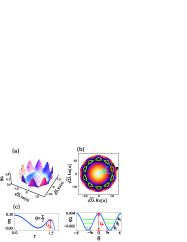
Figure 1: Quasienergy g in phase space. (a) $g\propto H_{R}$ versus Re$[a]$ and Im$[a]$ for power $n=10$ and driving strength $\mu=0.4\mu_{c}$. For nonzero driving, the quasienergy is invariant under discrete phase space rotations $e^{i\theta}\rightarrow e^{i(\theta+\tau)}$ where $\tau=2\pi/n$. (b) A cut through the bottom of the quasienergy $g$ in (a). There are $n$ stable states (yellow closed curves) and $n$ saddle points (unstable states, between two stable states) arranged periodically in angular direction. A local coordinate system $(x,p)$ is defined near the bottom of a stable state. (c) Quasienergy $g$ versus radius $r$ (left) and angle $\theta$ (right). Stable states are confined by the radial potential barrier $U_{r}$ and the angular potential barrier $U_{\theta}$. For the latter, we plot two wells between $\theta=-\tau$ and $\theta=\tau$. The localized states confined in each well (green lines) are coupled by quantum tunneling.

We assume that the driving frequency $\omega_{d}$ is close to $n$ times $\omega_{0}$; i.e., the detuning $\delta\omega\equiv\omega_{0}-\omega_{d}/n$ is much smaller than $\omega_{0}$. We perform a unitary transformation of the Hamiltonian $H(t)$ via $\hat{U}=e^{i({\omega_{d}}/{n})\hat{a}^{\dagger}\hat{a}t}$, where $\hat{a}$ is the annihilation operator of the oscillator. Dropping fast oscillating terms, in the spirit of the rotating wave approximation (RWA), we arrive at the time-independent Hamiltonian

$$\hat{H}_{R}=\hbar\delta\omega{\hat{a}^{\dagger}}\hat{a}+\frac{3\nu\hbar^{2}}{4m^{2}\omega_{0}^{2}}{\hat{a}^{\dagger}}\hat{a}({\hat{a}^{\dagger}}\hat{a}+1)+f\Big{(}\frac{\hbar}{2m\omega_{0}}\Big{)}^{\frac{n}{2}}\Big{(}{\hat{a}^{\dagger n}}+\hat{a}^{n}\Big{)}.$$ (2)

Although RWA is widely used in the study of driven systems, it is not immediately clear that it is valid for highly nonlinear coupling (e.g., $\sim q^{n}$). To test it, we performed an exact numerical simulation based on the full Floquet theory, not relying on the approximation, and present the results in the Supplemental Material. The conclusion is that as long as $|\delta\omega|/\omega_{0}<2\lambda$ (see the definition of $\lambda$ below) the RWA is well justified.

Discrete symmetry.— The RWA Hamiltonian Eq.(2) displays a new symmetry not visible in Eq.(1). To illustrate it, we first make use of a semiclassical approximation, replacing the operator $\hat{a}$ by a complex number, and plot the resulting Hamiltonian ${H}_{R}$ (2) in the phase space spanned by Re$[a]$ and Im$[a]$. The results, seen in Figs. 1(a) and  1(b), clearly display the discrete angular periodicity of ${H}_{R}$. For the following theoretical analysis, we define a unitary operator $\hat{T}_{\tau}=e^{-i\tau{\hat{a}^{\dagger}}\hat{a}}$ with the properties $\hat{T}_{\tau}^{\dagger}\hat{a}\hat{T}_{\tau}=\hat{a}e^{-i\tau}$ and $\hat{T}_{\tau}^{\dagger}\hat{a}^{n}\hat{T}_{\tau}=\hat{a}^{n}e^{-in\tau}$. It is easy to see that the RWA Hamiltonian is invariant under discrete transformation $T_{\tau}^{\dagger}\hat{H}_{R}T_{\tau}=\hat{H}_{R}$ for $\tau={2\pi}/{n}$.

The discrete angular symmetry suggests introducing the radial and angular operators $\hat{r}$ and $\hat{\theta}$ via $\hat{a}=e^{-i\hat{\theta}}\hat{r}/\sqrt{2\lambda}$ and $\hat{a}^{\dagger}=\hat{r}e^{i\hat{\theta}}/\sqrt{2\lambda}$. They obey the commutation relation

$$[\hat{r}^{2},e^{i\hat{\theta}}]=2\lambda e^{i\hat{\theta}}$$ (3)

where $\lambda=-3\nu\hbar/(4m^{2}\omega_{0}^{2}\delta\omega)$ is the scaled dimensionless nonlinearity. Using this definition, we get $\hat{H}_{R}=-(\hbar\delta\omega/\lambda)\hat{g}$, with

$$\hat{g}=\frac{1}{4}(\hat{r}^{2}+\lambda-1)^{2}+\frac{1}{2}\,\mu\,\left[\left({\hat{r}e^{i\hat{\theta}}}\right)^{n}+\left({e^{-i\hat{\theta}}\hat{r}}\right)^{n}\right].$$ (4)

The dimensionless driving strength is

$$\mu=-\frac{2\lambda f}{\hbar\delta\omega}\left(\frac{m\omega_{0}\delta\omega}{-3\nu}\right)^{n/2}.$$

For red detuning, $\delta\omega<0$, considered in the following $\mu>0$.

Semiclassical analysis.— We first analyze the properties of the phase space crystal in the semiclassical limit $\lambda$$\rightarrow$ $0$. For vanishing driving $\mu=0$, the quasienergy $g$ is independent of the angle $\theta$, which means $g$ is invariant under continuous phase space rotation. However, for finite driving $\mu\neq 0$, the quasienergy $g$ is only invariant under discrete phase space rotations $e^{i\theta}\rightarrow e^{i(\theta+\tau)}$ with $\tau=2\pi/n$. The periodic arrangement of atoms in a crystal replaces the continuous translation symmetry by a discrete one. Similarly, in a phase space crystal the stable points break the continuous rotation symmetry, and define the periodicity for the phase space crystal. In Fig. 1(b), the stable points are the $n$ minima $(r_{m},\theta_{m})$ of $g$. Between every two neighboring stable points there is a saddle point $(r_{s},\theta_{s})$.

In the vicinity of stable points, the quasienergy $g$ creates effective potential barriers for angular and radial motion $U_{\theta}$ and $U_{r}$, respectively. Both are shown in Fig. 1(c). Because of thermal or quantum fluctuations, the states may jump or tunnel between neighboring stable points across or through the angular potential with height $U_{\theta}\approx 2\mu$. The tunneling determines the band structure to be discussed below. In the Supplemental Material, we show that the height of the radial potential barrier $U_{r}$ decreases as the driving $\mu$ increases, up to a critical driving strength $\mu_{c}=(1-r^{2}_{c})/(nr^{n-2}_{c})$ with $r^{2}_{c}=(n-2)/(n-4)$, above which the stable points disappear. In the limit of large $n$, we find $\mu_{c}\approx{2}/[{\rm e}n(n-2)],$ where ${\rm e}$ is the Euler constant. In the following, we assume $\mu<\mu_{c}$ to guarantee the existence of stable points.

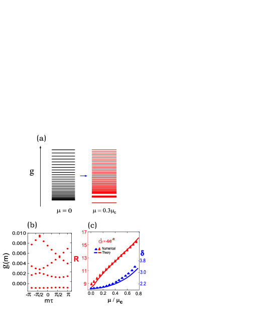
Figure 2: Quasienergy band structure. (a) Quasienergy spectrum changing from quasicontinuous in the absence of driving (left) to a band structure induced by finite driving (right). The gaps start to open from the bottom of the spectrum. (b) Quasienergy band structure in the reduced Brillouin zone. Each red dot represents one quasienergy level. There are $n$ levels in each band. (c) Width of the lowest band $d_{1}$, and the asymmetry factor $\delta$ versus driving. Numerical (triangles) and approximate (lines) results are compared. The parameters are $\lambda=1/205$, $n=10$ for all the figures, and for (b) we choose $\mu=0.3\mu_{c}$.

Quasienergy band structure.— In the quantum regime, $\hat{r}$ and $\hat{\theta}$ no longer commute. In Fig. 2(a), we show the eigenvalue spectrum of the quasienergy Hamiltonian obtained from a numerical diagonalization. In the limit of vanishing driving $\mu\rightarrow 0$, the spectrum is quasicontinuous whereas for $\mu\neq 0$ gaps open from the bottom of the spectrum. According to Bloch’s theorem, the eigenstates $\psi_{m}(\theta)$ of the quasienergy Hamiltonian $\hat{g}\psi_{m}(\theta)=g(m)\psi_{m}(\theta)$ have the form $\psi_{m}(\theta)=\varphi_{m}(\theta)e^{-im\theta}$, with a periodic function $\varphi_{m}(\theta+\tau)=\varphi_{m}(\theta)$. Here, the integer number $m$, which we call a ”quasinumber”, plays the role of the quasimomentum $\overset{\rightharpoonup}{\vphantom{a}\smash{k}}$ in a crystal. Whereas the quasimomentum $\overset{\rightharpoonup}{\vphantom{a}\smash{k}}$ is conjugate to the coordinate, the quasinumber $m$ is conjugate to the phase $\theta$. In Fig. 2(b), we plot the quasienergy band structure in the reduced Brillouin zone $m\tau\in(-\pi,\pi]$. Here, we relabel the eigenstates $\psi_{m}(\theta)$ by $\psi_{lm}(\theta)$, where $l=1,2,...$ is the label of the bands counted from the bottom. For finite values of $n$ (in our numerical simulation we chose $n=10$), the quasienergy band spectrum is discrete. It would become more continuous in the limit of large $n$.

(i) Band gaps.— The band structure is characterized by band gaps and bandwidths. If the driving is weak, $\mu\ll\mu_{c}$, only the first gap is visible. The gaps between higher bands are too narrow to distinguish them from the level spacings due to finite $n$. In perturbation expansion, we find for the first gap and bandwidth $\Delta_{1}\approx\mu$ and $d_{1}\approx{\lambda^{2}n^{2}}/{4}-{\mu}/{2}+{\mu^{2}}/({2\lambda^{2}n^{2}})$, respectively. I.e., the gap $\Delta_{1}$ increases linearly with the driving, whereas the bandwidth $d_{1}$ decreases with driving. For stronger driving, the spectrum of the $l$th band is approximately

$$g_{l}(m)=E_{l}-2|J_{l}|\cos(m\tau+\delta\tau),$$ (5)

centered around $E_{l}$ and with bandwidth $d_{l}=4|J_{l}|$. The result shows a surprising asymmetry. From the plot of the quasienergy in Fig. 1(b), we would have expected a degeneracy $g(m)=g(-m)$, since clockwise and anticlockwise motion should be equivalent, as in the case of orbital motion. However, in the present case, the two degrees of freedom of phase space Im$[a]$ and Re$[a]$ do not commute, and as a result the quasienergy structure is asymmetric. The degree of asymmetry is characterized in Eq. (5) by the asymmetry factor $\delta$.

In the case of sufficiently strong driving, several levels are localized in each stable point, as shown by Fig. 1(c) (right figure). The band structure can be explained by a tight-binding model: the gaps are opened by level spacings of localized states at the same stable point, whereas the bandwidth is determined by quantum tunneling between nearest neighbors. At the bottom of each stable point, to lowest order, the localized Hamiltonian can be approximated by a harmonic form with effective frequency $\omega_{e}=\left\{\mu n^{2}r_{m}^{n-2}[3r_{m}^{2}-1-n(n-1)\mu r_{m}^{n-2}]\right\}^{1/2}$ (see the Supplemental Material). Since $r_{m}\approx 1$, the localized quantum level spacing is $\lambda\omega_{e}\approx n\lambda\sqrt{2\mu}$. The level spacing corresponds to the distance between two centers of adjacent bands. The anharmonicity leads to higher-order corrections to the level spacings, for levels close to the bottom proportional to $-l\lambda^{2}$, where $l$ is the label of the band. This negative correction means that higher level spacings decrease linearly. The tight-binding approximation is valid for a $\mu>\lambda\omega_{e}/2$, where the angular potential barrier $U_{\theta}\approx 2\mu$ is high enough to confine at least one quantum level in each stable point.

(ii) Asymmetry factor.— The most unusual feature of the band structure (5) is the asymmetry characterized by the factor $\delta$. It results from the following property of the operator $\hat{r}^{2}$: in $\theta$ representation, one could conclude that the operator $\hat{r}^{2}$ with form $-i2\lambda{\partial}/{\partial\theta}$ satisfies the commutation relation (3) exactly. However, in this case the eigenvalues of $\hat{r}^{2}$ could be negative, which would be unphysical. We, therefore, define a local coordinate system $(x,p)$ measured from the bottom of a stable point as shown in Fig. 1(b). In the limit of large $n$, we have local operators $\hat{x}\approx\bar{r}(\hat{\theta}-\tau/2)$ and $\hat{p}=\hat{r}-\bar{r}$, where $\bar{r}$ is the average radius. Their commutation relation is $[\hat{p},\hat{x}]=i\lambda$. Thus, in “$x$ representation” , we have $\hat{p}=i\lambda({\partial}/{\partial x}),$ and $\hat{r}=\bar{r}+\hat{p}=\bar{r}+i\lambda({\partial}/{\partial x})$. Dropping the $\lambda^{2}$ term, we get $\hat{r}^{2}\approx\bar{r}^{2}+2i\lambda\bar{r}({\partial}/{\partial x})$. As a result, the first term of quantum quasienergy Hamiltonian (4) becomes $[2i\lambda\bar{r}({\partial}/{\partial x})+\bar{r}^{2}+\lambda-1]^{2}/4$, which indeed distinguishes anticlockwise and clockwise direction since $\bar{r}^{2}+\lambda-1\neq 0$ in general. In addition, the driving term in the Hamiltonian (4) introduces some asymmetry by changing the average radius $\bar{r}$.

We can explicitly calculate the asymmetry factor $\delta$ in the frame of the tight-binding model. The relation between the Bloch eigenstate $\psi_{lm}(\theta)$ and the localized state in each stable point $\phi_{l}(\theta)$, as indicated in Fig. 1(c), is given by $\psi_{lm}(\theta)=1/\sqrt{n}\sum_{q=0}^{n-1}e^{imq\tau}{\hat{T}_{\tau}^{q}}\phi_{l}(\theta)$. Only the nearest neighbor coupling $J_{l}=-\int[\hat{T}_{\tau}\phi_{l}(\theta)]^{*}\hat{g}\phi_{l}(\theta)d\theta$, is important. From $\hat{T}_{\tau}\phi_{l}(\theta)\approx e^{-i\tau\bar{r}^{2}/2\lambda}\phi_{l}(\theta+\tau)$, it follows to be $J_{l}=-e^{i\tau\bar{r}^{2}/2\lambda}\int\phi_{l}^{*}(\theta+\tau)\hat{g}\phi_{l}(\theta)d\theta=|J_{l}|e^{i\tau\bar{r}^{2}/2\lambda}$. The corresponding quasienergy spectrum of the $l$th band then is $g_{l}(m)=\int_{0}^{2\pi}\psi^{*}_{lm}(\theta)\hat{g}\psi_{lm}(\theta)d\theta\approx E_{l}-J_{l}e^{im\tau}-J_{l}^{*}e^{-im\tau}=E_{l}-2|J_{l}|\cos(m\tau+\bar{r}^{2}\tau/2\lambda)$. Hence the asymmetry factor is $\delta=\bar{r}^{2}/2\lambda\ (\mathrm{mod}\ n)$. A similar phase shift for the tunneling amplitude has been found for the special case of the parametric oscillator ($n=2$) in Ref. ParametricTunneling, . For the bottom band, the average radius is $\bar{r}_{1}=1-\lambda/2+\sum_{k=1}^{\infty}\bar{c}_{2k}\mu^{2k}$ with average coefficient $\bar{c}_{2k}$ given in the Supplemental Material. To get the average radius of next higher levels, we use the quantization condition in phase space $(\bar{r}^{2}_{l+1}-\bar{r}^{2}_{l})\tau/2=\pi\lambda$.

In Fig. 2(c), we show the dependence of the asymmetry factor $\delta$ on the driving strength $\mu$, obtained in both the tight-binding calculation described above and from a numerical simulation. The asymmetry arises from the phase of the complex tunneling parameter $J_{l}=|J_{l}|e^{i\tau\bar{r}^{2}/2\lambda}$. The phase factor $\tau\bar{r}^{2}/2\lambda$ called Peierls phase peierlsphase1 ; peierlsphase2 has also been discussed as a possibility to realize artificial gauge fields peierlsphase2 ; artificialgauge1 for ultracold atoms. For optical lattices, there are already some proposals to create a controlled Peierls phase by synthesizing a one-dimensional effective Zeeman lattice artificialgauge2 or shaking the lattice peierlsphase1 . In the present case, the complex tunneling parameter $J_{l}$ naturally arises in the plane of the phase space.

(iii) Bandwidths.— The $l$th bandwidth is $d_{l}=4|J_{l}|$. To calculate the amplitude of the coupling $|J_{l}|$, we use the double-well potential model, as shown by the right plot in Fig. 1(c). For the analysis of quantum tunneling, the property of quasienergy near the saddle point ($r_{s},\theta_{s}$) is important. We move the local coordinate system $(x,p)$ defined above to the saddle point ($r_{s},\theta_{s}=0$). Now the local coordinates are given by $x\approx r_{s}\theta$ and $p=r-r_{s}$. To second order, the Hamiltonian near the saddle point can be approximated by

$$g\approx\frac{1}{2}m_{s}\omega^{2}_{s}p^{2}+\mu r^{n}_{s}\cos(n\theta)+\frac{(r^{2}_{s}-1)^{2}}{4},$$ (6)

where $m_{s}\omega^{2}_{s}=\partial^{2}g/\partial r^{2}|_{(r_{s},\theta_{s})}$. Given an energy level $E_{l}$, one can write $|p|$ as a function of $\theta$ and calculate the amplitude of the coupling

$$|J_{l}|=\frac{\lambda\omega_{e}}{2\pi}\exp[-\frac{r_{s}}{\lambda}\int_{-\theta_{a}}^{\theta_{a}}|p|d\theta].$$ (7)

Here, $\theta_{a}$ is the turning point that is given by $\theta_{a}=1/n\cos^{-1}[(E_{l}-{(r^{2}_{m}-1)^{2}}/{4})/\mu r^{n}_{m}]$. The integral in the exponent of Eq. (7) is given by

$$\int_{-\theta_{a}}^{\theta_{a}}|p|d\theta=\frac{4}{n}\Big{\{}\frac{2}{m_{s}\omega^{2}_{s}}\Big{[}\mu r^{n}_{s}+\frac{(r^{2}_{s}-1)^{2}}{4}-E_{l}\Big{]}\Big{\}}^{1/2}E(\phi|k),$$ (8)

where $E(\phi|k)=\int_{0}^{\phi}\{1-k^{2}\sin^{2}\theta\}^{1/2}d\theta$ is the elliptic integral of the second kind with parameters $\phi=n\theta_{a}/2$ and $k=\left\{2\mu r^{n}_{s}/[\mu r^{n}_{s}+{(r^{2}_{s}-1)^{2}}/{4}-E_{l}]\right\}^{1/2}$. In Fig. 2(c), we compare our approximate result for the first bandwidth $d_{1}$ versus driving $\mu$ to numerical results. In the tight-binding regime they agree well with each other.

Emission spectrum.— The above calculation of quasienergy band structure does not account for a dissipative environment. It renders the time evolution of phase space crystal nonunitary and induces transitions between quasienergy states MarkOldDDO ; ParametricActivated . For a driven quantum system, even at base temperature $T=0$ many quasienergy states can be excited and transitions between them will contribute to the emission spectrum ParametricSpectrum ; QuantumHeatingMeasured . The spectral density of the photons emitted by the driven resonator DDOspectrum follows from $S(\omega)=2\,\mathrm{Re}\int_{0}^{\infty}dt\,\langle a^{\dagger}(t)a\rangle_{\rm st}e^{-i\omega t}$.

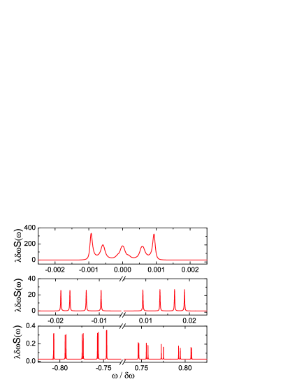
Figure 3: Emission spectrum: The top, middle and bottom figures are the emission spectrum for the first band, the second band and the interband respectively. The parameters: $\lambda=1/205$, temperature $\mathrm{T}=0.5\hbar\omega_{0}/k_{B}$, driving $\mu=0.4\mu_{c}$, the damping $\kappa=10^{-4}\lambda$.

To calculate the correlation function $C(t)=\langle a^{\dagger}(t)a\rangle_{\rm st}$, we need a master equation that also accounts for the dissipative evolution caused by thermal and quantum fluctuations. He have checked that a Lindblad-type master equation ParametricSpectrum ; MarkOldDDO ; LindbladME1 ; LindbladME2 ; LindbladME3 is sufficient for the present situation,

$$\frac{\partial\rho}{\partial\tau}=-\frac{i}{\lambda}[g,{\rho}]+\kappa(1+\bar{n}){\cal D}[a]{\rho}+\kappa\bar{n}{\cal D}[a^{\dagger}]{\rho}=\cal{L}\rho.$$ (9)

The dimensionless time $\tau=t\,\delta\omega$ is scaled by the detuning. The Lindblad superoperator is defined through ${\cal D}[A]{\rho}\equiv A{\rho}A^{\dagger}-(A^{\dagger}A{\rho}+{\rho}A^{\dagger}A)/2$ where $\bar{n}=(e^{\hbar\omega_{0}/k_{B}T}-1)^{-1}$ is the Bose distribution and $\kappa$ is the dimensionless damping scaled by the detuning. We make use of the quantum regression theorem to calculate the correlation function, i.e., $C(\tau)=\mathrm{Tr}[a^{\dagger}(\tau)a\rho_{\rm st}]=\mathrm{Tr}[a^{\dagger}e^{{\cal{L}}\tau}(a\rho_{\rm st})]$. The spectral density $S(\omega)$ is the Fourier transformation of the correlation function $C(\tau)$. We choose our parameters to confine two localized states in each well; i.e., we truncate our numerical simulation at $2n$ levels.

The total spectrum can be divided into three parts, as shown in Fig. 3. The top and middle figures represent intraband transitions of the first and second band, respectively. The bottom figure corresponds to interband transition between the first and second bands. The positive and negative frequencies in the emission spectrum correspond to absorption of energy from and emission of energy to the driving field, respectively. The widths of the peaks in emission spectrum are proportional to the damping $\kappa$. The quasienergy band structure can be directly detected by analyzing the spectrum of emitted photons in the laboratory. It should be noticed, however, that the above emission spectrum is obtained in the rotating frame with frequency $\omega_{d}/n$. Hence, a value of $\omega$ in this spectrum represents a photon with frequency $\omega+\omega_{d}/n$ in the laboratory frame.

Discussion.— The phase space crystal is a general consequence of a discrete rotation symmetry in phase space and is not restricted to the model presented in detail above. More generally it can be found for Hamiltonians such as $H(t)={{p}^{2}}/{2m}+m\omega_{0}^{2}q^{2}/2+V(q)+f(q)\cos(\omega_{d}t)$. For cold atoms, the nonlinear driving can be created by using power-law trapping methods. For trapped ions, it can be caused by an oscillating point charge coupling to the charged ion via Coulomb interaction, leading to the expansion $f(q)\propto 1/(1-q)=\sum^{\infty}_{k=0}q^{k}$. In the parameter range where RWA is valid (i.e., for $|\delta\omega|/\omega_{0}<2\lambda$ as derived in the Supplemental Material), in combination with the resonance condition $\omega_{d}\approx n\omega_{0}$, the driving term will automatically pick up terms $a^{n}$ and $a^{\dagger n}$ from $q^{n}$, or terms $a^{\dagger}a^{n+1}$ and $a^{\dagger n+1}a$ from $q^{n+2}$, etc. All these RWA terms remain invariant under discrete phase space rotation $e^{i\theta}\rightarrow e^{i(\theta+2\pi/n)}$. In the model analyzed above, we further assumed a nonlinear static potential $V(q)=\nu q^{4}/2$. Also, this can be chosen to be more general. If $V(q)$ is an even function of coordinate $q$, the RWA terms with equal numbers of $a^{\dagger}$ and $a$ will contribute to the phase space crystal.

In the solid-state band theory, the spectrum ultimately becomes continuous due to the large number of atoms. For the phase space crystal, a continuous quasienergy spectrum would emerge in the limit of large $n$. Compared to conventional artificial materials, such as photonic crystals, the energy band structure of phase space crystals can be changed in situ by tuning the driving field’s parameters. By changing the coupling power $n$, one can even change the lattice constant $\tau=2\pi/n$ of the phase space crystal. The new symmetry introduces the quasinumber space. The concept of quasinumber space may bring a new perspective to modify properties of materials.

Acknowledgements.— We acknowledge helpful discussions with P. Kotetes, J. Michelsen and V. Peano. L. Guo acknowledges the support from the China Scholarship Council.

Supplemental Material

.1 Justification for RWA

To derive Eq.(2) in the main text we adapted the well-known rotating wave approximation (RWA). The main results in this paper were derived within this approximation. In this section we perform an exact numerical simulation based on the full Floquet theory and calculate the quasienergy spectrum. We find the condition for the validity of RWA but also show numerical results beyond the RWA regime. We also discuss the role of non-RWA terms in the phase space crystal.

We start from the original time-dependent Hamiltonian in laboratory frame

$$\hat{H}(q,t)=\frac{{p}^{2}}{2m}+\frac{1}{2}m\omega_{0}^{2}q^{2}+\frac{\nu}{2}q^{4}+2f\cos(\omega_{d}t){q}^{n}.$$ (10)

We transform to the rotating frame via $\hat{U}=e^{i({\omega_{d}}/{n})\hat{a}^{\dagger}\hat{a}t}$ and keep all the terms

$$\hat{H}_{RF}(t)=\hat{U}\hat{H}(t)\hat{U}^{\dagger}+i\hbar\dot{\hat{U}}\hat{U}^{\dagger}=\hat{H}_{RWA}+\hat{H}_{non-RWA}.$$ (11)

The first part is the RWA Hamiltonian $\hat{H}_{RWA}=-(\hbar\delta\omega/\lambda)\hat{g}$ given by Eq.(2) and Eq.(4) in the main text. The non-RWA part Hamiltonian $\hat{H}_{non-RWA}$ has the following form

$$\hat{H}_{non-RWA} = \frac{\nu\hbar^{2}}{4m^{2}\omega_{0}^{2}}(2{\hat{a}^{\dagger}}\hat{a}-1)\hat{a}^{\dagger 2}e^{i{2\omega_{d}t}/{n}}+\frac{\nu\hbar^{2}}{8m^{2}\omega_{0}^{2}}\hat{a}^{\dagger 4}e^{i{4\omega_{d}t}/{n}}$$ (12)

$$+f\Big{(}\frac{\hbar}{2m\omega_{0}}\Big{)}^{\frac{n}{2}}\Big{[}\Big{(}{\hat{a}^{\dagger}e^{i{2\omega_{d}t}/{n}}}+\hat{a}\Big{)}^{n}-\hat{a}^{n}\Big{]}+\textit{h.c.}.$$

It is time-dependent, but the total Hamiltonian $\hat{H}_{RF}(t)$ is periodic, $\hat{H}_{RF}(t)=\hat{H}_{RF}(t+T)$, with period $T=2\pi/(2\omega_{d}/n)=n\pi/\omega_{d}$. In the framework of Floquet theory, the solution of Schrödinger equation $i\hbar\frac{\partial}{\partial t}|\Psi(t)\rangle=\hat{H}_{RF}(t)|\Psi(t)\rangle$ has the form $|\Psi(t)\rangle=e^{-i\epsilon t/\hbar}|\psi(t)\rangle$, where $|\psi(t)\rangle$ is the Floquet state satisfying $|\psi(t)\rangle=|\psi(t+T)\rangle$Floquettheory . Then the Schrödinger equation becomes

$$\mathscr{H}(t)|\psi(t)\rangle=\epsilon|\psi(t)\rangle.$$ (13)

Here, $\mathscr{H}(t)=\hat{H}_{RF}(t)-i\hbar\frac{\partial}{\partial t}$ is the Floquet Hamiltonian and $\epsilon$ is termed the quasienergy.

In order to calculate the quasienergy spectrum, we need to diagonalize the Floquet Hamiltonain $\mathscr{H}(t)$. Because of the periodicity $\mathscr{H}(t)=\mathscr{H}(t+T)$, it is convenient to introduce a composite Hilbert space $\mathscr{R}\otimes\mathscr{T}$, where $\mathscr{R}$ is the spatial space with the time-independent basis $|\phi_{m}\rangle\in\mathscr{R}$, which are determined by the eigenstates of RWA Hamiltonian $\hat{g}$

$$\hat{g}|\phi_{m}\rangle=g_{m}|\phi_{m}\rangle,$$ (14)

while $\mathscr{T}$ is the space of functions with time periodicity $T$. We can choose the time-dependent Fourier vectors $\langle t|q\rangle=\exp(iq\frac{2\omega_{d}}{n}t)$ with $q=0,\pm 1,\pm 2,\ldots,$ as the orthonormal basis of space $\mathscr{T}$. We denote the eigenstates and eigenvalues of the Floquet Hamiltonian $\mathscr{H}(t)$ by $|\psi_{m,q}(t)\rangle$ and $\epsilon_{m,q}$,

$$\mathscr{H}(t)|\psi_{m,q}(t)\rangle=\epsilon_{m,q}|\psi_{m,q}(t)\rangle.$$ (15)

Under the RWA, it is easy to see that $|\psi_{m,q}(t)\rangle=e^{-iq\frac{2\omega_{d}}{n}t}|\phi_{m}\rangle$ and $\epsilon_{m,q}=-(\hbar\delta\omega/\lambda)g_{m}+{2q\hbar\omega_{d}}/{n}$, i.e., for $q\neq 0$, the quasienergy spectrum is shifted by ${2q\hbar\omega_{d}}/{n}$.

Eq.(13) has infinitely many equivalent solutions. This is because the Floquet state $|\psi(t)\rangle$ is allowed to be time-dependent. After a time-dependent gauge transformation, the state $e^{-iq\frac{2\omega_{d}}{n}t}|\psi(t)\rangle$ is still a solution of Eq.(13), with corresponding quasienergy shifted Floquettheory by ${2q\hbar\omega_{d}}/{n}$, that is,

$$\mathscr{H}(t)\Big{(}e^{-iq\frac{2\omega_{d}}{n}t}|\psi(t)\rangle\Big{)}=(\epsilon+{2q\hbar\omega_{d}}/{n})\Big{(}e^{-iq\frac{2\omega_{d}}{n}t}|\psi(t)\rangle\Big{)},$$

where $q=0,\pm 1,\pm 2,\ldots,$. Thus we can map all the states with $q\neq 0$ to the state with $q=0$. The full form of this eigenstate $|\psi_{m,0}(t)\rangle$ with time-dependent Fourier expansion is

$$|\psi_{m,0}(t)\rangle=C^{0}_{m}|\phi^{0}_{m}\rangle+\sum_{m^{\prime},q\neq 0}C_{m^{\prime}q}e^{iq\frac{2\omega_{d}}{n}t}|\phi_{m^{\prime}}\rangle.$$ (16)

The corresponding quasienergy will also be modified, that is, $\epsilon_{m,0}=-(\hbar\delta\omega/\lambda)g_{m}+\Delta_{m}$. Here, the renormalized state $|\phi^{0}_{m}\rangle$ is in general a superposition of spatial basis states $|\phi_{m}\rangle$. The first term on the right side of Eq.(16) is a time-independent term which represents the RWA part while the second term of Eq.(16) represents the contribution from non-RWA Hamiltonian $\hat{H}_{non-RWA}$. Thus quantity $P_{0}=|C^{0}_{m}|^{2}$ is the probability for the RWA part of the full state.

Both the RWA probability $P_{0}$ and the quasienergy $\epsilon_{m,0}$ are functions of the detuning $\delta\omega$. As long as it is small enough, $|\delta\omega|/\omega_{0}\ll 1$, the RWA works well, which means $P_{0}\approx 1$ and $\epsilon_{m,0}\approx-(\hbar\delta\omega/\lambda)g_{m}$. However, for stronger detuning more and more higher order oscillating modes should be included as indicated by the sum in the second term of Eq.(16). By exact numerical simulation, we can calculate the relationship between $P_{0}$ and detuning as shown in Fig. 4a). We see that there is a critical point $|\delta\omega_{c}|$ for each $\lambda$ (see the definition of $\lambda$ in the main text). When the absolute value of detuning is smaller than the critical value, i.e., $|\delta\omega|<|\delta\omega_{c}|$, the RWA is well justified. The critical value $|\delta\omega_{c}|$ depends on the parameter $\lambda$. We can use the following simple method to estimate its value. Since the RWA Hamiltonian can be written as $\hat{H}_{RWA}=-(\hbar\delta\omega/\lambda)\hat{g}$, where $\hat{g}$ is a scaled dimensionless quantity, the prefactor $-(\hbar\delta\omega/\lambda)\equiv\hbar|\delta\omega|/\lambda$ (we assume a red detuning, $\delta\omega<0$) represents the energy scale of RAW Hamiltonian. In the non-RWA Hamiltonian $\hat{H}_{non-RWA}$, the lowest oscillating frequency is $2\omega_{d}/n$. Thus, the valid regime for the RWA can be estimated by the following condition

$$\hbar|\delta\omega|/\lambda<2\hbar\omega_{d}/n\Longrightarrow|\delta\omega|/(\omega_{d}/n)\approx|\delta\omega|/\omega_{0}<2\lambda.$$ (17)

The above condition means the critical point is $|\delta\omega_{c}|=2\lambda\omega_{0}$. On the plot of Fig. 1a), we indicate the critical points calculated from condition (17) for different $\lambda$’s by vertical dashed lines. They agree with numerical results very well.

In the main text, we show that the quasienergy band structure comes from the discrete angular rotation symmetry in phase space. This symmetry is a property of the RWA Hamiltonian. The non-RWA Hamiltonian $\hat{H}_{non-RWA}$, however, does not have this discrete symmetry. In fact, the existence of $\hat{H}_{non-RWA}$ will deteriorate the discrete angular rotation symmetry, thus modify the band structure of the quasienergy spectrum. As shown in Fig. 1b), large detuning tends to reduce the bandgap and broaden the bandwidth. But for a large region beyond the RWA regime, the band structure is very robust to the detuning (the bandwidth stays much smaller than the bandgap). We may consider non-RWA terms to behave like “disorder” in a phase space crystal. Further investigation of these effects will be independent future work. We also notice that the bandgap shows some peaks with changing detuning, and the bandwidth shows dips accordingly. For an explanation of these peaks beyond RWA see the work by V. Peano et al. BeyondRWA .

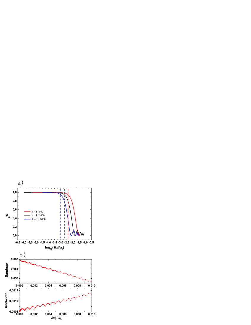
Figure 4: The role of strong detuning. a) The probability of the RWA part, $P_{0}$, of the full Floquet state (see Eq.(16)) versus detuning for different values of $\lambda$. Each level exhibits almost the same behavior against detuning for a fixed $\lambda$. The three colored vertical dashed lines indicate the critical values according to condition (17). b) The relationships between the bandgap (top) and the bandwidth (bottom), in units of $\hbar\omega_{d}/n$, as functions of detuning for $\lambda=1/2000$. Here, we plot the banddap and bandwidth of the first band. In fact, every band shows a similar behavior v.s. detuning. For stronger detuning more higher order oscillating modes should be included in the expansion of Eq.(16).

.2 Stability Analysis

We calculate the extrema of quasienergy in phase space by standard stability analysis. These extrema are classified into stable points and saddle points (unstable points). In semiclassical limit $\lambda\rightarrow 0$, the quasienergy is

$$g=\frac{1}{4}(r^{2}-1)^{2}+\mu r^{n}\cos(n\theta).$$ (18)

The extrema $(r_{e},\theta_{e})$ in angular and radial direction can be obtained from

$$\frac{\partial g}{\partial\theta}\big{|}_{\theta=\theta_{e},r=r_{e}} = -\mu nr_{e}^{n}\sin(n\theta_{e})=0$$ (19)

$$\frac{\partial g}{\partial r}\big{|}_{\theta=\theta_{e},r=r_{e}} = r_{e}[(r_{e}^{2}-1)+\mu nr_{e}^{n-2}\cos(n\theta_{e})]=0\,.$$ (20)

The two equations have a trivial solution $r_{e}=0$. In addition nontrivial solutions of the angular dependence can be obtained from Eq.(19), namely $\theta_{e}=l\tau/2$ with $l=0,\pm 1,\pm 2,...,\pm(n-1),n$, where $\tau=2\pi/n$ is defined as lattice constant of the phase space crystal. The corresponding radial extrema can be obtained from Eq.(20)

$$r_{e}=1+\sum_{k=1}^{\infty}c_{k}(\theta_{e})\mu^{k}.$$ (21)

Here, the series expansion coefficient $c_{k}(\theta)$ are given by

$$c_{k}(\theta)=\frac{(-1)^{k}({n}/{2})^{k}\cos^{k}(n\theta)[k(n-2)-1]!!}{k![k(n-4)+1]!!}.$$ (22)

The stability of these extrema $(r_{e},\theta_{e})$ is determined by the second derivatives of $g$. If $({\partial^{2}g}/{\partial\theta}^{2})\times({\partial^{2}g}/{\partial r}^{2})\big{|}_{r=r_{e},\theta=\theta_{e}}>0$, the extrema are stable, otherwise unstable. From

$$\frac{\partial^{2}g}{\partial\theta^{2}}\big{|}_{\theta=\theta_{e},r=r_{e}}=-\mu n^{2}r_{e}^{n}\sin(n\theta_{e})\big{|}_{\theta=\theta_{e}}=-\mu n^{2}r_{e}^{n}\sin(l\pi).$$ (23)

we see that odd integers of $l$ give $({\partial^{2}g}/{\partial\theta}^{2})\big{|}_{\theta=\theta_{e}}>0$, while even integers of $l$ give $({\partial^{2}g}/{\partial\theta}^{2})\big{|}_{\theta=\theta_{e}}<0$. The second derivative with repect to the radius $r$ is

$$\frac{\partial^{2}g}{\partial r^{2}}\big{|}_{r=r_{e},\theta=\theta_{e}}=3r^{2}_{e}-1+n(n-1)\mu\cos(n\theta_{e}).$$ (24)

For weak driving $\mu\ll 1$, since the radial extreme is $r_{e}\approx 1$, the above value is positive. From this we conclude that the angular extrema at $\theta_{m}=l\tau/2$ with $l$ odd integers between $-n$ and $n$ are stable points (minima), while the angular extrema at $\theta_{s}=l\tau/2$ with $l$ even integers between $-n$ and $n$ are unstable saddle points.

As the driving strength $\mu$ increases the condition (24) can reduce to zero, which means the nontrivial solutions of Eq.(20) disappear. The critical driving $\mu_{c}$ is determined by

$$\frac{\partial g}{\partial r}\big{|}_{\mu=\mu_{c}}=0,\ \ \ \ \ \mathrm{and}\ \ \ \ \ \frac{\partial^{2}g}{\partial r^{2}}\big{|}_{\mu=\mu_{c}}=0.$$ (25)

Solving the above two equations, we get $\mu_{c}=(1-r^{2}_{c})/(nr^{n-2}_{c})$ with $r^{2}_{c}=(n-2)/(n-4)$. In the limit of large $n$, the critical driving $\mu_{c}\approx{2}/[en(n-2)],$ where $e$ is the Euler constant.

.3 Local Hamiltonian

In this section, we give a perturbative form of the Hamiltonian close to the bottom of the stable points $(r_{m},\theta_{m})$. The eigenvalues and eigenstates of the local Hamiltonian are needed for the tight-binding calculation. We first write the local Hamiltonian in a harmonic approximation

$$g_{local} \approx \frac{1}{2}\frac{\partial^{2}g}{r^{2}_{m}\partial\theta^{2}}\big{|}_{(r_{m},\theta_{m})}(r_{m}\theta-r_{m}\theta_{m})^{2}$$ (26)

$$+\frac{1}{2}\frac{\partial^{2}g}{\partial r^{2}}\big{|}_{(r_{m},\theta_{m})}(r-r_{m})^{2}+g(r_{m},\theta_{m})$$

$$= \frac{p^{2}}{2m_{e}}+\frac{1}{2}m_{e}\omega^{2}_{e}x^{2}+\frac{(r^{2}_{m}-1)^{2}}{4}-\mu r_{m}^{n}.$$

Here, we have defined the coordinate $x=r-r_{m}$ and momentum $p=r_{m}(\theta-\theta_{m})$ near the stable point. The effective mass $m_{e}$ and effective frequency $\omega_{e}$ are given by $m_{e}=r_{m}^{2}({\partial^{2}g}/{\partial\theta^{2}})^{-1}$ and $\omega_{e}=\sqrt{m^{-1}_{e}{\partial^{2}g}/{\partial r^{2}}}$ respectively, with explicit formulars $m_{e}=(\mu n^{2}r_{m}^{n-2})^{-1},\ \ \omega_{e}=\sqrt{\mu n^{2}r_{m}^{n-2}[3r_{m}^{2}-1-n(n-1)\mu r_{m}^{n-2}]}.$

The anharmonicity gives higher order corrections to the localized Hamiltonian. We transform the original $\hat{g}$ to a local Hamiltonian $\hat{g}_{local}$ at the stable point $(r_{m},\theta_{m})$ by three steps. Firstly, we change the orientation using the phase space rotation operator $\hat{T}_{\theta_{m}}=e^{-i\theta_{m}{\hat{a}^{\dagger}}\hat{a}}$, resulting in a properly orientated Hamiltonian $\hat{T}_{\theta_{m}}\hat{g}\hat{T}^{\dagger}_{\theta_{m}}$. Secondly, we move $\hat{T}_{\theta_{m}}\hat{g}\hat{T}^{\dagger}_{\theta_{m}}$ to the position of stable point using the displacement operator $\hat{D}_{\alpha}=e^{\alpha a^{\dagger}-\alpha^{*}a}$, resulting in a Hamiltonian sitting at the bottom of stable point $\hat{D}_{\alpha}\hat{T}_{\theta_{m}}\hat{g}\hat{T}^{\dagger}_{\theta_{m}}\hat{D}^{\dagger}_{\alpha}$. Finally, we squeeze the Hamiltonian to fit the stable point by using the squeezing operator $\hat{S}_{\xi}=e^{[\xi^{*}a^{2}-\xi(a^{\dagger})^{2}]/2}$, resulting in the needed local Hamiltonian $\hat{g}_{local}=\hat{S}_{\xi}\hat{D}_{\alpha}\hat{T}_{\theta_{m}}\hat{g}\hat{T}^{\dagger}_{\theta_{m}}\hat{D}^{\dagger}_{\alpha}\hat{S}^{\dagger}_{\xi}$.

The displacement operator $\hat{D}_{\alpha}$ has the property $D_{\alpha}^{\dagger}aD_{\alpha}=a+\alpha$, while the squeezing operator $\hat{S}_{\xi}$ satisfies $S_{\xi}^{\dagger}aS_{\xi}=va+ua^{\dagger}$, where $v=\cosh|\xi|,\ \ u=-\xi/|\xi|\sinh|\xi|$ are the squeezing parameters. Starting from the following original form of $\hat{g}$

$$\hat{g}=\frac{1}{4}(2\lambda\hat{a}^{\dagger}\hat{a}+\lambda-1)^{2}+\frac{1}{2}\mu(2\lambda)^{\frac{n}{2}}\Big{(}{\hat{a}^{\dagger n}}+\hat{a}^{n}\Big{)},$$ (27)

and choosing the parameters $\alpha=-r_{e}/\sqrt{2\lambda}$, $v=(\sqrt{m_{e}\omega_{e}}+1/\sqrt{m_{e}\omega_{e}})/2$, and $u=(\sqrt{m_{e}\omega_{e}}-1/\sqrt{m_{e}\omega_{e}})/2$ we get the local Hamiltonian

$$\hat{g}_{local} = \hat{S}_{\xi}\hat{D}_{\alpha}\hat{T}_{\theta_{m}}\hat{g}\hat{T}^{\dagger}_{\theta_{m}}\hat{D}^{\dagger}_{\alpha}\hat{S}^{\dagger}_{\xi}$$

$$= \lambda\omega_{e}(\hat{a}^{\dagger}\hat{a}+\frac{1}{2})+\frac{(r^{2}_{m}-1)^{2}}{4}-\mu r_{m}^{n}+\lambda^{3/2}\Delta\hat{g}+o(\lambda^{2}).$$

The term $\Delta\hat{g}=(v-u)r_{e}((v\hat{a}^{\dagger}-u\hat{a})(v\hat{a}-u\hat{a}^{\dagger})+1/2)(\hat{a}+\hat{a}^{\dagger})/\sqrt{2}-n(n-1)(n-2)\mu r_{e}^{n-3}(v\hat{a}^{\dagger}-v\hat{a})^{3}/(3\sqrt{2})+c.c.$ is treated in perturbation theory. In this way we can determine the local quantum level to order $\lambda^{2}$.

.4 Average radius $\bar{\textit{{r}}}$

In order to get the asymmetry factor $\delta$, we need to calculate the average radius $\bar{r}$. In the limit of large $n$, we define a local coordinate system $(x,p)$ near the bottom of stable points with corresponding operators defined by $\hat{x}=\bar{r}(\hat{\theta}-\tau/2)$ and $\hat{p}=\hat{r}-\bar{r}$, where $\bar{r}$ is the average radius. They satisfy the commutation relation $[\hat{p},\hat{x}]=i\lambda$. In “$x$-representation” or “$\theta$-representation”, we have $\hat{p}=i\lambda\frac{\partial}{\partial x}=i\frac{\lambda}{\bar{r}}\frac{\partial}{\partial\theta}.$ Then we have $\hat{r}^{2}/(2\lambda)=(\bar{r}+\hat{p})^{2}/(2\lambda)=(\bar{r}^{2}+2i\lambda\frac{\partial}{\partial\theta}-\lambda^{2}\frac{\partial^{2}}{\partial\theta^{2}})/(2\lambda)$. Neglecting terms of order $\lambda^{2}$, we get an important relationship $\hat{r}^{2}/(2\lambda)\approx\bar{r}^{2}/(2\lambda)+i\frac{\partial}{\partial\theta}$.

The average radius of the bottom band, $\bar{r}_{1}$, can be estimated by averaging $r_{e}(\theta)$, given by Eq.(21), over the angular direction $\bar{r}_{1}=\frac{1}{2\pi}\int_{0}^{2\pi}r_{e}(\theta)d\theta.$ Since $\overline{\cos^{k}(n\theta)}=\frac{1}{2\pi}\int_{0}^{2\pi}\cos^{k}(n\theta)d\theta={(k-1)!!}/{k!!}$ for even integer $k$ and $\overline{\cos^{k}(n\theta)}=0$ for odd integer $k$, we have from Eq.(22)

$$\bar{c}_{2k}=(-\frac{n}{2})^{2k}\frac{(2k-1)!![2k(n-2)-1]!!}{(2k)!!(2k)![2k(n-4)+1]!!}.$$ (29)

The average radius of the bottom band is given by $\bar{r}_{1}=1+\sum_{k=1}^{\infty}\bar{c}_{2k}\mu^{2k}$. This result is obtained based on the semiclassical quasienergy (18). Considering quantum correction, the final result is $\bar{r}_{1}=1-\lambda/2+\sum_{k=1}^{\infty}\bar{c}_{2k}\mu^{2k}$. This approximation is justified by our numerical simulation.

References

• (1) J. Zhang et al. Nature Commun. 2, 574 (2011).
• (2) J. R. Beresford, Band Structure Engineering for Electron Tunneling Devices, Columbia University, 1990.
• (3) P. M. Koenraad and M. E. Flatt$\mathrm{\acute{e}}$, Nature Materials 10, 91-100 (2011).
• (4) Y. Nishi and R. Doering, Handbook of Semiconductor Manufacturing Technology. Marcel Dekker Inc., 2000.
• (5) F. Guinea, M. I. Katsnelson and A. K. Geim, Nature Physics 6, 30-33 (2010).
• (6) K. S. Novoselov et al., Science 306, 666-669 (2004).
• (7) F. Yavari et al., Small 6, 2535-2538 (2010).
• (8) E. V. Castro et al., Phys. Rev. Lett. 99, 216802 (2007).
• (9) J. D. Joannopoulos, P. R. Villeneuve and S. Fan, Nature 386, 143-149 (1997).
• (10) E. Yablonovitch, Phys. Rev. Lett. 58, 2059-2062 (1987); E. Yablonovitch et al., Phys. Rev. Lett. 67, 2295-2298 (1991).
• (11) S. John, Phys. Rev. Lett. 58, 2486-2489 (1987).
• (12) Z. V. Vardeny, A. Nahata and A. Agrawal, Nature Photonics 7, 177-187 (2013).
• (13) E. L. Thomas, T. Gorishnyy and M. Maldovan, Nature Materials 5, 773-774 (2006).
• (14) M. Choi et al., Nature 470, 369-373 (2011).
• (15) J. T. Shen, P. B. Catrysse and S. Fan, Phys. Rev. Lett. 94, 197401 (2005).
• (16) N. Fang et al., Nature Materials 5, 452-456 (2006).
• (17) M. Grifoni and P. Hänggi, Phys. Rep. 304, 229 (1998).
• (18) J. H. Shirley, Phys. Rev. 138, 4B, 979 (1965)
• (19) Y. B. Zeldovitch, Sov. Phys. JETP 24 (1967) 1006 [Zh. Eksp. Teor. Fiz. 51 (1966) 1492].
• (20) Z. Gu et al., Phys. Rev. Lett. 107, 216601 (2011).
• (21) B. H. Wu et al., Appl. Phys. Lett. 100, 203106 (2012).
• (22) E. S. Morell and Luis E. F. Foa Torres, Phys. Rev. B 86, 125449 (2012); H. L. Calvo et al., Appl. Phys. Lett. 98, 232103 (2011); H. L. Calvo et al., Appl. Phys. Lett. 101, 253506 (2012).
• (23) A. Gómez-León and G. Platero, Phys. Rev. Lett. 110, 200403 (2013).
• (24) N. H. Lindner et al., Nature Physics 7, 490-495 (2011).
• (25) C. Stambaugh and H. B. Chan, Phys. Rev. Lett. 97, 110602 (2006).
• (26) H. B. Chan and C. Stambaugh, Phys. Rev. B 73, 224301(2006).
• (27) M. I. Dykman, Zh. Eksp. Teor. Fiz. 68, 2082 (1975).
• (28) M. I. Dykman, Phys. Rev. E 57 , 5202 (1998).
• (29) M. Marthaler and M. I. Dykman, Phys. Rev. A 76, 010102(R) (2007).
• (30) P. W. H. Pinkse et al., Phys. Rev. Lett. 78, 990-993 (1997)
• (31) D. M. Stamper-Kurn et al., Phys. Rev. Lett. 81, 2194-2197 (1998)
• (32) Franco Dalfovo et al., Rev. Mod. Phys. 71, 463-512 (1999)
• (33) V. Bagnato, D. E. Pritchard, and D. Kleppner, Phys. Rev. A 35, 4354 (1987).
• (34) A. Jaouadi, et al., Phys. Rev. A 82, 023613 (2010); A. Jaouadi, et al., Phys. Rev. A 83, 023616 (2011).
• (35) Guozhen Su, Jincan Chen, and Lixuan Chen, Physics Letters A 315 (2003) 109-19.
• (36) Shukuan Cai,et al., Physica A 387 (2008) 4814-820.
• (37) Berna Gülveren, Solid State Sciences 14 (2012),94-99.
• (38) J. Struck et al., Phys. Rev. Lett. 108, 225304 (2012)
• (39) N. Goldman et al.,arXiv:1308.6533
• (40) Jean Dalibard et al., Rev. Mod. Phys. 83,1523-1543 (2011)
• (41) K. Jiménez-García, et al., Phys. Rev. Lett. 108, 225303 (2012)
• (42) M. I. Dykman and V. N. Smelyanskiy, Zh. Eksp. Teor. Fiz. 94, 61 (1988).
• (43) M. Marthaler and M. I. Dykman, Phys. Rev. A 73, 042108 (2006).
• (44) M. I. Dykman, M. Marthaler and V. Peano, Phys. Rev. A 83, 052115 (2011).
• (45) S. André, L. Guo, V. Peano, M. Marthaler and G. Schön, Phys. Rev. A 85, 053825 (2012).
• (46) F. R. Ong et al., Phys. Rev. Lett. 110, 047001 (2013).
• (47) L. Guo et al., Phys. Rev. E 84, 011144 (2011)
• (48) S. Diehl et al., Phys. Rev. Lett. 105, 015702 (2010).
• (49) M. I. Dykman, Phys. Rev. E 75, 011101 (2007).
• (50) V. Peano, M. Marthaler, and M. Dykman, Phys. Rev. Lett. 109, 090401 (2012).