Screening and gap generation in bilayer graphene

Abstract

A fully selfconsistent treatment for gap generation and Coulomb screening in excitonic insulators is presented. The method is based on the equations of motion for the relevant dynamical variables combined with a variational approach. Applying the theory for a model system of bilayer graphene, an excitonic groundstate with a gap exceeding 10 meV is predicted.

I Introduction

With the discovery and rise of graphene and graphene based systems, the interest in the spontaneous formation of an excitonic groundstate has been revived. It has been noticed already in the 1960’s that electron–electron interactions in narrow-gap semiconductors or semi-metals may lead to an instability of the normal groundstateJérome et al. (1967); Halperin and Rice (1968). If the noninteracting gap is smaller than the exciton binding energy, excitons may form spontaneously and the system is expected to undergo a phase transition into an excitonic state in close analogy to the BCS superconductor. In contrast to the BCS superconductor, however, the pairing in the narrow-gap semiconductors occurs between oppositely charged particles leading to an excitonic insulator state. Its quasiparticle spectrum exhibits a gap exceeding that of the noninteracting groundstate and it has a characteristic “Mexican hat”-like shape, displaying the spontaneously broken symmetry of the interacting groundstateJérome et al. (1967)

Since its first theoretical proposal, the experimental and theoretical search for material systems hosting this interesting state of matter has been a subject of continuous researchJérome et al. (1967); Halperin and Rice (1968); Littlewood and Zhu (1996); Butov (2004); Eisenstein and MacDonald (2004). The ideal host combines a small gap with a large exciton binding and high stability with respect to external perturbations.

As a consequence of its zero-gap single-particle bandstructure, single-layer graphene (SLG) seems a promising candidate for an excitonic insulator. Due to the linear dispersion SLG exhibits massless, chiral Dirac Fermions which attracted significant interest recently. In particular, the formal analogy between spontaneous exciton condensation and chiral symmetry breaking in QED has been discussed by several authorsSemenoff (1984); Khveshchenko (2009); Wang and Liu ; Zhang et al. (2011); Semenoff (2012); Kotov et al. (2012).

The linear dispersion and chiral nature of the quasiparticles in SLG leads to fundamental differences in the effects of e–e interactions as compared to the conventional two-dimensional electron gas (2DEG). Recent analysisGrönqvist et al. (2012) of the Wannier equation with a linear dispersion shows that exciton binding in SLG requires a minimum effective Coulomb coupling strength, in general agreement with other theoretical investigationsPereira et al. (2007); Shytov et al. (2007a, b); Gamayun et al. (2009, 2010); Sabio et al. (2010); Wang et al. (2010); Stroucken et al. (2011); Drut and Lähde (2009a, b); González (2012); Kotov et al. (2012).

The actual strength of the Coulombic coupling in SLG is still a subject of debateHwang and Das Sarma (2007); Gamayun et al. (2010); Reed et al. (2010); González (2012); Kotov et al. (2012); González (2012); Gonzalez . Combination of the static limit of the standard Lindhard formula with experimentally measured values for the Fermi velocity predicts values for the Coulombic coupling that are slightly larger than the critical value, thus allowing for a small but finite gap. However, despite intense investigations, so far no experimental evidence has been presented for the occurrence of a gap in the SLG spectrum.

Recently, also bilayer graphene (BLG) has attained much interest. Combining two graphene sheets to a so called A–B or Bernal stacked bilayer, the interlayer tunneling changes the linear dispersion into a quadratic one, preserving the band degeneracy at the Dirac points and the chiral nature of the quasiparticlesMcCann (2006); McCann et al. (2007); Nilsson et al. (2008). As such, BLG is a very interesting system, exhibiting simultaneously similarities and differences in its excitonic and screening properties as compared to SLG and the 2DEG. Specifically, the massive quasiparticles lead to bound excitons for arbitrarily weak Coulomb attractionZhang et al. (2010); Vafek and Yang (2010); Nandkishore and Levitov (2010) and hence, BLG is expected to host an excitonic groundstate. Moreover, as has been predicted theoretically and demonstrated experimentallyMcCann (2006); McCann et al. (2007); Stauber et al. ; Liang and Yang , a tunable gap can be introduced by applying a gate bias or perpendicular electric field and hence, BLG provides the ideal model system to study exciton condensation.

As has been emphasized by several authors, the predictions for gap generation and exciton condensation depend sensitively on the model used for screening. In the existing literature, dynamical screening has mainly been studied within the standard RPA or one-loop approximationHwang and Das Sarma (2008); Sensarma et al. (2010); Zhang et al. (2010); Vafek and Yang (2010); Gamayun (2011); Nandkishore and Levitov (2010). Within the standard RPA, the bare bubble polarization describes virtual transitions across the Fermi level. The prediction for the screening depend on the occupation numbers of the involved states, their dispersion and overlap matrix elements. Unlike in conventional materials where the bandstructure is fixed by the crystalline structure, in an excitonic insulator it depends on the strength of the Coulomb interaction itself, and hence, the screening and gap calculations have to be done selfconsistently.

In this paper, we develop a framework that is capable to treat gap generation and screening on equal footing. Our method is based on the equations of motion for the dynamical variables that are solved in the static limit. In the regime of weak Coulomb coupling, our method produces a self-energy correction to the single particle energies and the standard bare bubble polarization. In the regime of strong Coulomb coupling, our results predict the opening of a gap in the quasiparticle spectrum that suppresses effective screening.

We use our method to analyze the excitonic instability in BLG. For this purpose, we adopt a two-band continuum model that neglects trigonal warping and intervalley interactions. The numerical evaluations predict a gap of roughly 14 meV for freely suspended BLG. For each valley degree of freedom, the corresponding state displays a broken layer symmetry, leading to a charge polarization. States with a charge polarization in opposite directions are degenerate.

The paper is organized as follows: In Sec. II, we present our model Hamiltonian for the BLG system. In Sec. III, we discuss the screened gap equations and in Sec. IV we summarize our numerical results. A detailed derivation of the screened gap equations is given in the App. A.

II Bilayer model Hamiltonian

As a model system, we consider BLG in Bernal stacking, as shown schematically in Fig. 1. The two coupled layers have hexagonal carbon lattic structures with sites $A1$, $B1$ and $A2$, $B2$ located at $z_{1}$ and $z_{2}$ respectively. In the Bernal stacking, the in-plane coordinates of the $B1$ and $A2$ layers coincide, but those of $A1$ and $B2$ do not. Within a single layer, only nearest neighbor hopping is taken into account and characterized by the hopping parameter $\gamma_{0}=2.8$ eV, which is related to the Fermi velocity by $3\gamma_{0}b/2\equiv\hbar v_{F}$ where $b=1.41$Å is the carbon–carbon distance. Interlayer hopping between the sites B1 and A2 is characterized by the hopping parameter $\gamma_{1}=0.39$ eV and that between $A1$ and $B2$ by $\gamma_{2}=0.32$ eV, respectively. Hence, the free-particle part of the Hamiltonian is given by

$$H_{0}=\sum_{{\bm{k}}}\hat{\Psi}^{\dagger}_{{\bm{k}}}\begin{pmatrix}0&\gamma_{0}f({{\bm{k}}})&0&\gamma_{1}\cr\gamma_{0}f^{*}({{\bm{k}}})&0&\gamma_{2}f^{*}({{\bm{k}}})&0\cr 0&\gamma_{2}f({{\bm{k}}})&0&\gamma_{0}f({{\bm{k}}})\cr\gamma_{1}&0&\gamma_{0}f^{*}({{\bm{k}}})&0\end{pmatrix}\hat{\Psi}_{{\bm{k}}}$$ (1)

where $\hat{\Psi}_{{\bm{k}}}^{\dagger}=(a_{1,{\bm{k}}}^{\dagger},b_{1,{\bm{k}}}^{\dagger},a_{2,{\bm{k}}}^{\dagger},b_{2,{\bm{k}}}^{\dagger})$ is a 4-component field operator combining the creation operators in the 4 sublattices and $f({{\bm{k}}})=\sum_{i=1}^{3}e^{i{{\bm{k}}}\cdot{\bm{b}}_{i}}$ reflects the symmetry of the hexagonal lattice, see Fig. 1. Within the first Brillouin zone, $f({{\bm{k}}})$ has two nonequivalent roots ${\bm{K}}^{\pm}=(2\pi/3b,\pm 2\pi/3\sqrt{3}b)$ defining the two Dirac points.

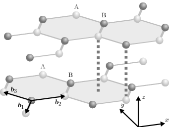
Figure 1: Schematic illustration of the bilayer graphene lattice in Bernal stacking. The lattice consists of two honeycomb structures separated by a distance $L$ and rotated with respect to each other. Each single layer is characterized by the three vectors ${\bm{b}}_{i}$ connecting a carbon atom of the $A$ layer with its three nearest neighbors.

Diagonalization of the single-particle Hamiltonian gives four bands, two of them being degenerate at the Dirac points and two of them shifted by $\gamma_{1}$, see Fig. 2. Hence, in the energy range $E<\gamma_{1}$, the single-particle part of the effective Hamiltonian can be described within a two-band approximation, with contributions arising from regions in the Brillioun zone that are centered around the two Dirac points. If we define the wavenumber with respect to the Dirac points and distinguish the respective Dirac points by the valley index $\tau=\pm$, each valley component contributes equally, giving

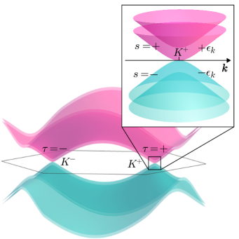
Figure 2: Schematic illustration of the bilayer bandstructure within the tight-binding model. Two of the four bands are degenarate at the Dirac points $K^{\pm}$, labeled by the valley index $\tau$. The inset shows a zoom in at the $K^{+}$ point. The degenerate bands are labeled by the band index $s=\pm 1$ and have energies $\epsilon_{s{\bm{k}}}=s\epsilon_{{\bm{k}}}$, respectively.

$$H_{0}=\sum_{\tau,s,{\bm{k}}}\epsilon_{s,{\bm{k}}}c_{\tau,s,{\bm{k}}}^{\dagger}c_{\tau,s,{\bm{k}}}.$$ (2)

Here, $c^{\dagger}_{\tau,s,{\bm{k}}}$ creates an electron with band index $s$ and wavenumber ${\bm{K}}^{\tau}+{\bm{k}}$. Within the two-band approximation, the symmetric conduction and valence bands are conveniently labeled by $s=\pm 1$ with $\epsilon_{s,{\bm{k}}}=s\epsilon_{{\bm{k}}}$. The corresponding Bloch waves consist of components on the interacting $B1$ and $A2$ sublattices localized on the lower and upper sheet, respectively. A detailed derivation of the projection procedure is given in App. B. Close to the Dirac points, the effect of the trigonal warping is negligible and the energy dispersion of the symmetric bands can be approximated by the relativistic dispersion

$$\epsilon_{{\bm{k}}}=\sqrt{\left(mv_{F}^{2}\right)^{2}+(\hbar v_{F}k)^{2}}-mv_{F}^{2}$$ (3)

with the rest mass $m=\gamma_{1}/(2v_{F}^{2})$ determined by the interlayer hopping.

As we are interested in collective system properties on a length scale larger than the lattice spacing, we include the Coulomb interaction within the continuum model and neglect intervalley scattering requiring a momentum transfer $|{\bm{q}}|>\frac{4\pi}{3\sqrt{3}b}$. Using a $k$-space representation for the in-plane coordinates and keeping the full $z$ dependence, the Coulomb Hamiltonian is

$$H_{C} = \frac{1}{2}\frac{e^{2}}{\epsilon_{B}}\sum_{{\bm{q}}\neq 0}V_{0}({\bm{q}})\iint dzdz^{\prime}\,\hat{\rho}_{{\bm{q}}}(z){\rm e}^{-q|z-z^{\prime}|}\hat{\rho}_{-{\bm{q}}}(z^{\prime})$$ (4)

$$= \frac{1}{2}\frac{e^{2}}{\epsilon_{B}}\sum_{{\bm{q}}\neq 0}\sum_{ij}V_{0}^{ij}({\bm{q}})\hat{\rho}^{i}_{{\bm{q}}}\hat{\rho}^{j}_{-{\bm{q}}}.$$

Here, $V_{0}({\bm{q}})=2\pi/(qNA)$ is the two-dimensional (2D) Coulomb potential, $NA$ is the normalization area, and $\epsilon_{B}$ is the dielectric constant of the substrate. Furthermore,

$$\hat{\rho}_{{\bm{q}}}(z) = \sum_{{{\bm{k}}}}\sum_{\tau,ss^{\prime}}W_{\tau,ss^{\prime}}({\bm{k}},{\bm{q}},z)c^{\dagger}_{\tau,s,{\bm{k}}-{\bm{q}}}c_{\tau,s^{\prime},{\bm{k}}}$$ (5)

$$\equiv \sum_{i=1,2}\hat{\rho}^{i}_{{\bm{q}}}f({{\bm{q}}},z-z_{i})$$

is the effective density operator projected onto the lowest bands,

$$W_{\tau,ss^{\prime}}({\bm{k}},{\bm{q}},z)=\frac{1}{2}\bigl{[}{\rm e}^{-i\tau(\phi_{{\bm{k}}}-\phi_{{\bm{k}}-{\bm{q}}})} f({{\bm{q}}},z-z_{1})$$

$$+ss^{\prime}{\rm e}^{i\tau(\phi_{{\bm{k}}}-\phi_{{\bm{k}}-{\bm{q}}})} f({{\bm{q}}},z-z_{2})\bigr{]}$$

is the wave function overlap, and $f({\bm{q}},z)=\int_{e.c.}d^{2}\rho{\rm e}^{-i{\bm{q}}\cdot\bm{\rho}}|\phi(\bm{r})|^{2}$ is the in-plane Fourier transform of the electron density corresponding to the atomic orbitals. Within the tight-binding (TB) approximation, the total charge density can be divided into the contributions $\rho^{i}$, located in layer $i$. The Coulomb potential between the carriers in sheet $i$ and $j$ is

$$V_{0}^{ij}({\bm{q}}) =V_{0}({\bm{q}})\iint\!\!dzdz^{\prime}\,f({\bm{q}},z-z_{i}){\rm e}^{-q|z-z^{\prime}|}f(-{\bm{q}},z^{\prime}-z_{j})$$

$$=V_{0}({\bm{q}})H(q,|z_{i}-z_{j}|)\,.$$ (6)

As shown in App. C, $H(q,L)\equiv\tilde{H}(qd,L/d)$ depends on the effective thickness $d$ of a single graphene sheet and the interlayer spacing $L$. These intrinsic length scales should be compared to the excitonic Bohr radius

$$a_{0}=\frac{\hbar^{2}\epsilon_{B}}{me^{2}}=3\frac{\gamma_{0}}{\gamma_{1}}\frac{b}{\alpha}$$

where $\alpha=e^{2}/(\epsilon_{B}\hbar v_{F})$ is the effective fine structure constant. If $d/a_{0}<<1$, finite size effects on the excitonic properties can be neglected and the system can be considered as effectively 2D. Within this limit, the Hamiltonian scales strictly with the exciton Bohr radius and depends on the parameter combination $\alpha$ characterizing the importance of relativistic effects. In the nonrelativistic limit $\alpha\ll 1$, the BLG dispersion is approximately quadratic and the only relevant energy unit is the exciton Rydberg

$$E_{0}=\frac{me^{4}}{\epsilon_{B}^{2}\hbar^{2}}=\frac{1}{2}\alpha^{2}\gamma_{1}.$$

III Screened gap equations

To determine the groundstate of our model Hamiltonian, we extend the methods derived in Stroucken et al. (2011) for SLG to treat gap generation and screening effects on equal footing. In the appendix, we present the technical details of our method that is valid for arbitrary narrow gap semiconductors and semimetals. Here, we only summarize the main derivation steps adapted specifically to the BLG model Hamiltonian.

In general, the effect of screening is described by the polarization function, describing the charge density induced by a density fluctuation. In an effectively 2D system, the charge density is homogeneous with respect to the in-plane coordinates but localized in the $z$ direction. For BLG, the charge localization invloves both layers leading to a matrix-like Coulomb potential $V^{ij}$ describing the interaction between particles located in the sheets $i$ and $j$, respectively. As the polarization results from the induced charge densities within the layers, it also has a $2\times 2$ matrix structure:

$$\Pi(\omega,{\bm{q}},z,z^{\prime}) = -\frac{i}{\hbar}\int_{0}^{\infty}dt{\rm e}^{i\omega t}\left<\left[\hat{\rho}_{{\bm{q}}}(z,t),\hat{\rho}_{-{\bm{q}}}(z)\right]\right>$$

$$= \sum_{i,j}f({\bm{q}},z-z_{i})\Pi^{ij}(\omega,{\bm{q}})f(-{\bm{q}},z^{\prime}-z_{j})\,.$$

The screened potential obeys the integral equation

$$V_{s}(\omega,{\bm{q}},z,z^{\prime})=V_{0}({\bm{q}},z-z^{\prime})$$

$$+\frac{e^{2}}{\epsilon_{\rm B}}\iint dz_{1}dz_{2}V_{0}({\bm{q}},z-z_{1})\Pi(\omega,{\bm{q}},z_{1},z_{2})V_{s}(\omega,{\bm{q}},z_{2},z^{\prime}).$$

Defining the screened interaction matrix

$$V_{s}^{ij}(\omega,{\bm{q}})=\iint dzdz^{\prime}f_{{\bm{q}}}(z-z_{i})V_{s}(\omega,{\bm{q}},z,z^{\prime})f_{-{\bm{q}}}(z^{\prime}-z_{j}),$$

the integral equation reduces to a much simpler matrix equation with the solution

$${\underline{\underline{V_{s}}}}(\omega,{\bm{q}}) = \left(\underline{\underline{I\!\!I}}-\frac{e^{2}}{\epsilon_{\rm B}}{\underline{\underline{V}}}_{0}({\bm{q}}){\underline{\underline{\Pi}}}(\omega,{\bm{q}})\right)^{-1}{\underline{\underline{V}}}_{0}({\bm{q}})$$ (9)

$$\equiv {\underline{\underline{\epsilon}}}(\omega,{\bm{q}})^{-1}{\underline{\underline{V}}}_{0}({\bm{q}}).$$

If the influence of the finite layer separation $L$ can be neglected, the interaction is independent of the layer indices and one obtains the standard 2D result

$$V_{s}^{2D}(\omega,{\bm{q}})=\frac{V_{0}({\bm{q}})}{1-\frac{e^{2}}{\epsilon_{\rm B}}V_{0}({\bm{q}})\Pi^{2D}(\omega,{\bm{q}})}$$ (10)

with $\Pi^{2D}(\omega,{\bm{q}})=\sum_{ij}\Pi^{ij}(\omega,{\bm{q}})$. The components of the dynamical polarization ${\underline{\underline{\Pi}}}(\omega,{\bm{q}})$ can be calculated from the microscopic equations of motion for the operator combinations $c^{\dagger}_{\tau,s,{\bm{k}}-{\bm{q}}}c_{\tau,s^{\prime},{\bm{k}}}$ that constitute the density operator.

Due to its specific mathematical structure as continued fraction, the polarization function can be divided into a dominant part and small corrections that can be treated perturbatively. In a weakly interacting system, a convenient choice for the dominant part is the noninteracting suceptibility, i.e. expectation values are taken with respect to the noninteracting groundstate. However, in a strongly interacting system, corrections due to the Coulomb interaction modify the system groundstate properties and cannot be treated perturbatively. Instead, the expectation value on the RHS of Eq. LABEL:densdensresponse has to be taken with respect to the interacting groundstate. Since the interacting groundstate depends on the strength of the Coulomb interaction that is in turn limited by screening effects, this constitutes a self-consistency problem.

In the absence of external perturbations, the system is homogeneous with respect to the in-plane coordinates and only single-particle operator combinations with ${\bm{k}}={\bm{k}}^{\prime}$, $\tau=\tau^{\prime}$ give nonzero expectation values. Hence, within a mean-field approximation, the unperturbed Hamiltonian consists of two independent contributions from each valley component which are related by the parity transformation or charge conjugation: $W_{+,ss^{\prime}}({\bm{k}},{\bm{q}},z)=W_{-,ss^{\prime}}(-{\bm{k}},-{\bm{q}},-z)=W^{*}_{-,ss^{\prime}}({\bm{k}},{\bm{q}},z)$. In the following, we suppress the valley index and perform explicit calculations for the ${\bm{K}}^{+}$ valley. As dynamical quantities, we use the microscopic intraband occupation numbers $f_{s,{\bm{k}}}=\langle c^{\dagger}_{s{\bm{k}}}c_{s{\bm{k}}}\rangle$ and the interband coherences $P_{{\bm{k}}}=\langle c^{\dagger}_{-{\bm{k}}}c_{+{\bm{k}}}\rangle$.

As shown in App. A, within the time dependent Hartree-Fock approximation, the equations of motion for all possible single-particle operator combinations $c^{\dagger}_{s{\bm{k}}-{\bm{q}}}c_{s^{\prime}{\bm{k}}}$ can be derived from the effective mean-field Hamilonian

$$\hat{H}^{\text{MF}}\!\! = \sum_{s,{\bm{k}}}\Sigma_{s,{\bm{k}}}c^{\dagger}_{s{\bm{k}}}c_{s{\bm{k}}}-\Omega_{{\bm{k}}}c^{\dagger}_{+.{\bm{k}}}c_{,-,{\bm{k}}}-\Omega^{*}_{{\bm{k}}}c^{\dagger}_{-,{\bm{k}}}c_{+,{\bm{k}}},$$

where

$$\Sigma_{s,{\bm{k}}} = \frac{\delta\langle H\rangle}{\delta f_{s{\bm{k}}}}=s\left(\epsilon_{{\bm{k}}}+\frac{e^{2}}{2\epsilon_{\rm B}}\sum_{{\bm{k}}^{\prime}}V_{s}^{\rm ND}({\bm{k}}-{\bm{k}}^{\prime}){\rm cos}(2(\phi_{{\bm{k}}}-\phi_{{\bm{k}}^{\prime}}))\left(f_{-,{\bm{k}}^{\prime}}-f_{+,{\bm{k}}^{\prime}}\right)\right.$$ (12)

$$- \left.i\frac{e^{2}}{2\epsilon_{\rm B}}\sum_{{\bm{k}}^{\prime}}V_{s}^{\rm ND}({\bm{k}}-{\bm{k}}^{\prime}){\rm sin}(2(\phi_{{\bm{k}}}-\phi_{{\bm{k}}^{\prime}}))\left(P_{{\bm{k}}^{\prime}}-P^{*}_{{\bm{k}}^{\prime}}\right)\right)-\frac{e^{2}}{2\epsilon_{\rm B}}\sum_{{\bm{k}}^{\prime}}V_{s}^{\rm D}({\bm{k}}-{\bm{k}}^{\prime})\left(f_{-,{\bm{k}}^{\prime}}+f_{+,{\bm{k}}^{\prime}}\right)$$

are the renormalized single-particle energies, and

$$\Omega_{{\bm{k}}} = -\frac{\delta\langle H\rangle}{\delta P^{*}_{{\bm{k}}}}=i\frac{e^{2}}{2\epsilon_{\rm B}}\sum_{{\bm{k}}^{\prime}}V_{s}^{\rm ND}({\bm{k}}-{\bm{k}}^{\prime}){\rm sin}(2(\phi_{{\bm{k}}}-\phi_{{\bm{k}}^{\prime}}))\left(f_{-,{\bm{k}}^{\prime}}+f_{+,{\bm{k}}^{\prime}}\right)$$ (13)

$$+ \frac{e^{2}}{2\epsilon_{\rm B}}\sum_{{\bm{k}}^{\prime}}V_{s}^{\rm D}({\bm{k}}-{\bm{k}}^{\prime})\left(P_{{\bm{k}}^{\prime}}+P^{*}_{{\bm{k}}^{\prime}}\right)-\frac{e^{2}}{2\epsilon_{\rm B}}\sum_{{\bm{k}}^{\prime}}V_{s}^{\rm ND}({\bm{k}}-{\bm{k}}^{\prime}){\rm cos}(2(\phi_{{\bm{k}}}-\phi_{{\bm{k}}^{\prime}}))\left(P_{{\bm{k}}^{\prime}}-P^{*}_{{\bm{k}}^{\prime}}\right)$$

is the internal field. The energy renormalizations and the internal field result from the exchange contributions of the two-particle interaction and are evaluated with the screened Coulomb potential. Here, we used the notation $V_{s}^{\rm D}=V_{s}^{11}=V_{s}^{22}$ for the intralayer and $V_{s}^{\rm ND}=V_{s}^{12}=V_{s}^{21}$ for the interlayer Coulomb interaction, respectively. The renormalized single-particle energies in Eq. 12 contain a constant, band independent contribution that corresponds to a shift of the Fermi energy which can be dropped from the equations.

Defining the Liouville operator by

$${\cal L}_{ss^{\prime}\sigma\sigma^{\prime}}({\bm{k}},{\bm{q}}) = \delta_{s\sigma}\delta_{s^{\prime}\sigma^{\prime}}\left(\Sigma_{s^{\prime},{\bm{k}}}-\Sigma_{s,{\bm{k}}-{\bm{q}}}\right)$$ (14)

$$- \delta_{s\sigma}\left(\delta_{s^{\prime}+}\delta_{\sigma^{\prime}-}\Omega_{{\bm{k}}}+\delta_{s^{\prime}-}\delta_{\sigma^{\prime}+}\Omega^{*}_{{\bm{k}}}\right)$$

$$+ \delta_{s^{\prime}\sigma^{\prime}}\left(\delta_{s+}\delta_{\sigma-}\Omega^{*}_{{\bm{k}}-{\bm{q}}}+\delta_{s-}\delta_{\sigma+}\Omega_{{\bm{k}}-{\bm{q}}}\right),$$

the time evolution of the density operator is given by

$$\hat{\rho}^{i}_{{\bm{q}}}(t) = \sum_{ss^{\prime}\sigma\sigma^{\prime}}\sum_{{\bm{k}}}W^{i}_{ss^{\prime}}({\bm{k}},{\bm{q}}){\rm e}^{-i{\cal L}_{ss^{\prime}\sigma\sigma^{\prime}}({\bm{k}},{\bm{q}})t/\hbar}c^{\dagger}_{\sigma{\bm{k}}-{\bm{q}}}c_{\sigma^{\prime}{\bm{k}}}$$

such that

$$\Pi^{ij}(\omega,{\bm{q}}) = {\cal N}\sum_{ss^{\prime}\sigma\sigma^{\prime}}\sum_{{\bm{k}}}W^{i}_{ss^{\prime}}({\bm{k}},{\bm{q}})\left[\hbar\omega{\cal E}-{\cal L}({\bm{k}},{\bm{q}})\right]^{-1}_{ss^{\prime}\sigma\sigma^{\prime}}$$ (16)

$$\times \left<\left[c^{\dagger}_{\sigma{\bm{k}}-{\bm{q}}}c_{\sigma^{\prime}{\bm{k}}},\hat{\rho}^{j}_{-{\bm{q}}}\right]\right>.$$

Here, ${\cal E}$ is the unity matrix and we included a degeneracy factor ${\cal N}=4$ to account for the spin and valley degrees of freedom. The expectation value of the equal time commutator can be evaluated, giving

$$\left<\left[c^{\dagger}_{\sigma{\bm{k}}-{\bm{q}}}c_{\sigma^{\prime}{\bm{k}}},\hat{\rho}^{j}_{-{\bm{q}}}\right]\right>=W_{\sigma\sigma^{\prime}}^{j*}({\bm{k}},{\bm{q}})\left(f_{\sigma,{\bm{k}}-{\bm{q}}}-f_{\sigma^{\prime},{\bm{k}}}\right)$$

$$+\delta_{\sigma-}W_{+\sigma^{\prime}}^{j*}({\bm{k}},{\bm{q}})P_{{\bm{k}}-{\bm{q}}}+\delta_{\sigma+}W_{-\sigma^{\prime}}^{j*}({\bm{k}},{\bm{q}})P^{*}_{{\bm{k}}-{\bm{q}}}$$

$$-\delta_{\sigma^{\prime}+}W_{\sigma-}^{j*}({\bm{k}},{\bm{q}})P_{{\bm{k}}}-\delta_{\sigma^{\prime}-}W_{\sigma+}^{j*}({\bm{k}},{\bm{q}})P^{*}_{{\bm{k}}}.$$

In general, the density-density response function describes the polarizability due to real and virtual transitions, exhibiting resonances at the transition energy between the involved states. For the interacting system, the poles of the polarization occur at $\omega=\pm(E_{s,{\bm{k}}-{\bm{q}}}-E_{s^{\prime},{\bm{k}}})$ where

$$E_{s,{\bm{k}}}=s\sqrt{\Sigma_{\bm{k}}^{2}+|\Omega_{\bm{k}}|^{2}}\equiv sE_{{\bm{k}}}$$ (18)

and $\Sigma_{{\bm{k}}}=(\Sigma_{+,{\bm{k}}}-\Sigma_{-,{\bm{k}}})/2$ is the spectrum of the mean-field Hamiltonian defined in Eq. LABEL:HMF. This Hamiltonian can be diagonalized by the Bogoliubov transformation with the Bogoliubov vacuum as groundstate.

Using the Bogoliubov representation, the mean-field Hamiltonian and the Liouville operator are diagonal in the band indices and the transition probability depends on the occupation numbers of the involved states and overlap matrix elements. Due to the Pauli exclusion, intraband transitions require partially filled bands and do not contribute to the groundstate polarization. Hence, within the Bogoliubov picture, the groundstate polarization is solely due to interband transitions. In a gapped system, these transitions require a finite transition energy $\hbar\omega\simeq E_{gap}$ and do not contribute to the static limit of the groundstate polarization. Moreover, due to the orthogonality of the Bloch waves with equal wavenumbers, the long-wavelength limit ${\bm{q}}\rightarrow 0$ of the interband contributions vanishes exactly in a gapped system and the long-ranged part of the static Coulomb interaction is essentially unscreened. However, if the system is ungapped, virtual interband transitions are not ruled out by energy conservation, leading to a finite groundstate polarization even in the static limit. Thus, the occurrence of a finite gap will reduce the effective screening of the long-ranged part of the static Coulomb interaction, and thus modifies the collective system properties significantly.

As can be recognized from Eq. 18, the Bogoliubov spectrum shows a gap if either the renormalized single-particle energy, or the internal field is nonzero at the Dirac points. For symmetry reasons, a nonvanishing energy renormalization at ${\bm{k}}=0$ requires anisotropic distributions, while a finite internal field can also be introduced by a real, isotropic distribution for the interband coherences. Physically, the real part of the macroscopic interband coherence $P=\sum_{{\bm{k}}}P_{{\bm{k}}}$ corresponds to a layer polarization, which can be seen from the average charge density given by

$$\rho_{{\bm{q}}=0}(z)=\frac{1}{2}\sum_{s{\bm{k}}}f_{s,{\bm{k}}}\left(f({\bm{q}}=0,z-z_{1})+f({\bm{q}}=0,z-z_{2})\right)$$

$$+\sum_{{\bm{k}}}\,\text{Re}\left[P_{{\bm{k}}}\right]\left(f({\bm{q}}=0,z-z_{1})-f({\bm{q}}=0,z-z_{2})\right).$$

Hence, a gap can be achieved e.g. by a static or time dependent external field that induces either an anisotropy, e.g. by photon absorption, or a layer polarization, e.g. by a static external field.

Here, we investigate the possibility for a spontaneous gap by exciton formation. A gapped state will emerge spontaneously if a symmetry breaking lowers the total energy of the interacting system.

Starting from an arbitrary mean-field state, an infinitesimal variation of the occupation numbers and the interband coherence yields an energy shift

$$\delta\langle H\rangle = \sum_{s{\bm{k}}}\Sigma_{s,{\bm{k}}}\delta f_{s,{\bm{k}}}-\sum_{{\bm{k}}}\left(\Omega_{{\bm{k}}}\delta P^{*}_{{\bm{k}}}+\Omega^{*}_{{\bm{k}}}\delta P_{{\bm{k}}}\right).$$ (19)

Assuming that the interacting groundstate is adiabatically connected to the noninteracting one, the constraint of a stationary solution implies (for a detailed derivation see App. A)

$$f_{+,{\bm{k}}} = 1-f_{-,{\bm{k}}}\equiv f_{{\bm{k}}}$$ (20)

$$|P_{{\bm{k}}}|^{2} = f_{{\bm{k}}}(1-f_{{\bm{k}}}),$$ (21)

giving

$$\delta\langle H\rangle = \sum_{{\bm{k}}}\left(2\Sigma_{{\bm{k}}}P_{{\bm{k}}}-(1-2f_{{\bm{k}}})\Omega_{{\bm{k}}}\right)\delta P^{*}_{{\bm{k}}}+c.c.,$$ (22)

which is negative if the Wannier equation has bound-state solutionsJérome et al. (1967); Grönqvist et al. (2012). The groundstate populations are determined by the variational principle $\delta<H>=0$, giving the algebraic relations

$$|P_{{\bm{k}}}| = \frac{1}{2}\frac{|\Omega_{{\bm{k}}}|}{E_{{\bm{k}}}}$$ (23)

$$f_{{\bm{k}}} = \frac{1}{2}\left(1-\frac{\Sigma_{{\bm{k}}}}{E_{{\bm{k}}}}\right).$$ (24)

Assuming real, isotropic distributions, insertion of these relations into the definitions for the internal field and renormalized energies gives the set of coupled integral equations:

$$\Omega_{{\bm{k}}}= \frac{e^{2}}{2\epsilon_{\rm B}}\sum_{{\bm{k}}^{\prime}}V_{s}^{\rm D}(|{\bm{k}}-{\bm{k}}^{\prime}|)\frac{\Omega_{{\bm{k}}^{\prime}}}{E_{{\bm{k}}^{\prime}}}$$ (25)

$$\Sigma_{{\bm{k}}}= \epsilon_{{\bm{k}}}+\frac{e^{2}}{2\epsilon_{\rm B}}\sum_{{\bm{k}}^{\prime}}V_{s}^{\rm ND}(|{\bm{k}}-{\bm{k}}^{\prime}|){\rm cos}2(\phi_{{\bm{k}}}-\phi_{{\bm{k}}^{\prime}})\frac{\Sigma_{{\bm{k}}^{\prime}}}{E_{{\bm{k}}^{\prime}}}.$$ (26)

The gap equations contain the statically screened Coulomb potential and must be solved selfconsistently with the static limit of the polarization function $\Pi^{ij}(\omega=0,{\bm{q}})$.

The gap equation Eq. 25 always has the trivial solution $P_{{\bm{k}}}=\Omega_{{\bm{k}}}\equiv 0$ corresponding to the noninteracting groundstate. If this trivial solution is unique, the interacting system has the same groundstate as the noninteracting one, i.e. we are in the limit of weak Coulomb coupling. The corresponding mean-field Hamiltonian is diagonal within the noninteracting picture, and hence, the Bogoliubov and noninteracting representations coincide.

The Bogoliubov quasiparticle spectrum is then equivalent to the renormalized single-particle energy:

$$\Sigma_{{\bm{k}}}=\epsilon_{{\bm{k}}}+\frac{e^{2}}{2\epsilon_{\rm B}}\sum_{{\bm{k}}^{\prime}}V_{s}^{\rm ND}(|{\bm{k}}-{\bm{k}}^{\prime}|){\rm cos}2(\phi_{{\bm{k}}}-\phi_{{\bm{k}}^{\prime}}),$$ (27)

and contains the renormalization by the filled valence band. Neglecting the effects of the finite thickness of the bilayer (i.e. putting $H(q,L)\approx 1$), this single-particle renormalization corresponds to that of the renormalization group (RG) approachGonzález et al. (1994); Vafek and Yang (2010). The corresponding noninteracting polarization function is given by the standard Lindhard formula with self energy corrections Hwang and Das Sarma (2008).

$$\Pi^{2D}_{0}(\omega,{\bm{q}}) = \sum_{ij}\Pi^{ij}_{0}(\omega,{\bm{q}})$$ (28)

$$= {\cal N}\sum_{{\bm{k}}}|W_{+-}({\bm{k}},{\bm{q}})|^{2}\left(\frac{1}{\hbar\omega-\left(\Sigma_{{\bm{k}}}+\Sigma_{{\bm{k}}-{\bm{q}}}\right)}\right.$$

$$- \left.\frac{1}{\hbar\omega+\left(\Sigma_{{\bm{k}}}+\Sigma_{{\bm{k}}-{\bm{q}}}\right)}\right).$$

If the gap equation has a nontrivial solution, it predicts a gap $|\Omega_{{\bm{k}}=0}|$ in the interacting quasiparticle spectrum. The corresponding state is energetically below the weakly coupled state and we shall refer to this state as strongly coupled (ground-) state. The gapped dispersion reduces the long wavelength limit of the static polarizability thus leading to a further increase of the predicted gap. Hence, though the noninteracting polarizability may be used as criterion for the occurence of an excitonic instability of the groundstate, to estimate the size of the gap screening and gap generation must be treated selfconsistently.

The strongly coupled state has a macroscopic layer polarization $P=\sum_{{\bm{k}}}\Omega_{{\bm{k}}}/2E_{{\bm{k}}}$. As can be recognized from Eq. 25, solutions with opposite layer polarizations are degenerate. As Eq. 25 is valid for both Dirac points, states where charge-polarization contributions from the two valley components are aligned or anti parallel are also degenerate such that a gapped state not necessarily exhibits a physical charge polarization. However, this degeneracy might be lifted by intervalley interactions which we neglected here.

IV Numerical results

The screened gap equations constitute a rather complicated set of integral equations that can be solved iteratively. In a first step, we evaluate the Lindhard formula in the noninteracting limit and insert this result into the gap equations. For any fixed polarization function, the screened gap equations are then solved by iterating candidates for the solution. After convergence, $f_{{\bm{k}}}$ and $P_{{\bm{k}}}$ are calculated from the solution of the gap equations and inserted into the generalized Lindhard formula Eq. 16, which is used to modify the Coulomb interaction. This procedure is repeated until overall convergence is achieved. All calculations have been performed in the limit of vanishing interlayer spacing $L\rightarrow 0$, which we verified to give correct results within the numerical accuracy for realistic values of $L$.

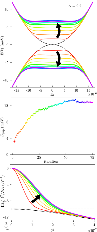
Figure 3: Iteration steps in the self-consistent solution of the screened gap equations (25), (26), with the screening (16). In the top panel, the quasiparticle dispersion (18) is shown, in the middle panel, the value of the gap at each step is plotted, and in the bottom panel, the polarizability is presented. Here, the screening in the unpopulated tight-binding bands using the full relativitic disperion is indicated by the dotted line, and the dashed line shows the constant value obtained in the noninteracting, nonrelativistic limit.

Fig. 3 shows the resulting spectra and polarization as functions of $kb$ in the vicinity of the Dirac points. In the calculations, we used $\alpha=2.2$, which is slightly below the nominal value for the coupling strength in vacuum. The individual lines refer to different numbers of iterations and the thick black arrows indicate the directions of convergence for increasing iteration numbers. The initial input values, corresponding to the noninteracting groundstate, are marked by the dotted lines. As can be recognized from the lowest panel of Fig. 3, the noninteracting polarizability overestimates the effects of screening, particularly in the long-wavelength limit $q\rightarrow 0$. As a result of the ungapped dispersion, virtual electron–hole pairs can be created practically without any cost of energy, leading to a very efficient intrinsic screening. In the long-wavelength limit, the noninteracting polarizability approaches the constant static polarization that is obtained if a purely quadratic dispersion is assumedHwang and Das Sarma (2008); Nandkishore and Levitov (2010). This result, indicated by the dashed line in the right panel of Fig. 3, turns into a linear curve for larger wavenumbers, similar to the noninteracting polarizability of SLG and characteristic for a linear dispersionHwang and Das Sarma (2007).

Since massive quasiparticles are sensitive to arbitrarily weak interactions, we find a nontrivial solution of the gap equations even if the Coulomb potential is screened by the noninteracting polarization function. The resulting quasiparticle spectrum is shown by the red line in the upper panel of Fig. 3 and exhibits a small but finite gap at the Dirac point. The opening of a gap immediately suppresses virtual transitions by means of energy conservation, leading to a practically unscreened long ranged tail of the Coulomb interaction. In the next step of iteration, this suppression of the screening enhances the gap, suppressing the screening and further enhancing the gap, and so on. Overall convergence is achieved after ca. 70 iterations, as shown in the middle panel of Fig. 3, where the gap is plotted against the number of iteration steps. Further iterations give values for the gap oscillating around its mean value by $\pm 5\%$, indicating the accuracy of our procedure.

The resulting spectrum exhibits a “Mexican hat” shape with band extrema slightly shifted away from the Dirac point, typical for an excitonic insulatorJérome et al. (1967). The $k$-values denoted by $k_{X}$, at which the band extrema occur, can be associated with a characteristic length scale which can be interpreted as excitonic correlation length. Between the band extrema, the dispersion is almost flat, while it approaches the noninteracting dispersion very rapidly for larger $k$-values. The size of the gap is approximately $E_{gap}\approx 12$ meV, which is well below the energy of the remote bands falling well within the region where the quadratic approximation is valid.

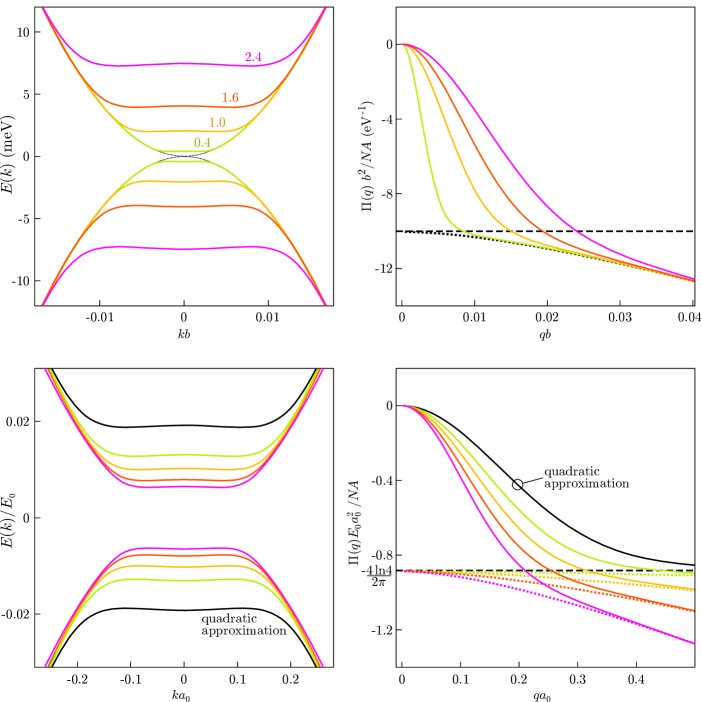
Figure 4: Bogoliubov dispersions and polarizabilities as obtained from the selfconsistently solved screened gap equations. The lines of different color correspond to the respective solutions for the values $\alpha=$ 2.4, 1.6, 1.0, and 0.4. The upper two panels show the solutions in absolute units, and the lower two in excitonic units, respectively. The panels on the right show the polarizabilities with zero populations as dotted lines. The dashed line shows the constant value obtained for zero populations in the quadratic approximation.

To analyze the dependence on the coupling strength, we plot in Fig. 4 the Bogoliubov spectra and the polarizabilities for various values of $\alpha$ in absolute and excitonic units. With increasing coupling strength, the characteristic wave number $k_{X}$ increases, corresponding to shorter excitonic correlation lengths. In the lower panel of Fig. 4, the same spectra are shown in excitonic units. Within the quadratic approximation, all energies scale with the excitonic energy unit and all curves merge into a universal one, indicated by the black line. Despite the small size of the gap, using the full relativistic dispersion shows clear deviations from this universal curve, with deviations increasing with increasing coupling strength.

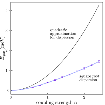
Figure 5: Quasiparticle gap vs. coupling strength as obtained from the selfconsistently solved screened gap equations. The thicker line shows the values obtained with the full relativisic dispersion (3), whereas the the thinner line indicates the results with a quadratic approximation for the dispersion.

The cause of these deviations can be found in the interplay between the two different length scales set by the Compton wavelength and the screening length of the massive quasiparticles. The Compton wavelength $\lambda_{c}=\hbar/mv_{F}=3\gamma_{0}b/\gamma_{1}$ involves only single-particle properties and $k\lambda_{c}\sim 1$ marks the crossover from the nonrelativistic quadratic into the relativistic linear dispersion. The screening length determines the range of the Coulomb interaction. Only if the screening length is large compared to the Compton wavelength, the Coulomb integrals converge within a wavenumber range where relativistic corrections to the dispersion can be neglected. Since the condition of simultaneous energy and momentum conservation is much less restrictive for the linear dispersion than for the quadratic one, the major effect of these corrections is an enhancement of screening effects.

The inverse screening length follows from the noninteracting polarization function via $\kappa=-2\pi e^{2}/\epsilon_{B}\lim_{q\rightarrow 0}\Pi_{0}(\omega=0,{\bm{q}})$ and is proportional to $e^{2}/\epsilon_{B}$, i.e. to the coupling constant. The long-wavelength limit of the noninteracting polarizability can be obtained analytically by assuming a purely quadratic dispersion, giving $\kappa={\cal N}{\rm ln}4/a_{0}$Hwang and Das Sarma (2008), where $a_{0}=\lambda_{c}/\alpha$ is the excitonic unit length. Hence, the ratio of the Compton wavelength and screening length $\kappa\lambda_{c}={\cal N}{\rm ln}4\alpha$ increases linearly with $\alpha$ and the validity of the quadratic approximation is limited to relatively weak interaction strengths $\alpha\lesssim({\cal N}{\rm ln}4)^{-1}$. As can be recognized from the right panels of Fig. 4, for larger values of the coupling constant, relativistic modifications to the dispersion enhance the effects of screening thus reducing the gap.

In Fig. 5, we plot the quasiparticle gap as function of coupling strength $\alpha$ for the full dispersion and the quadratic approximation, respectively. Using the quadratic approximation, the gap scales strictly with the exciton energy unit, i.e. with $\alpha^{2}$, as shown in App. C. Again, the comparison with the full solution shows that the quadratic approximation yields reasonable results only for small values of $\alpha$, while it overestimates the gap significantly if the interaction strength increases.

V Conclusions

In this paper, we present a selfconsistent approach to treat gap generation and screening in an effectively 2D excitonic insulator and applied our method to study the groundstate properties of bilayer graphene. To this end, we derive a generalization of the standard Lindhard formula that is based on the equations of motion for the density operator and is capable to describe the polarizability in a nondiagonal representation. To determine the groundstate properties, we solve the static limit of the generalized Lindhard formula selfconsistently with the gap equations, from which the groundstate populations and excitonic coherences are calculated.

Our method can be used on top of any effective single-particle band structure calculation. For a weakly coupled system, it reproduces the standard RPA result with self-energy corrections. In the strongly coupled regime, spontaneously formed coherent groundstate populations lead to the opening of a gap in the quasi-particle spectrum, with a corresponding suppression of the long-wavelength limit of the polarizability. This mechanism leads to an enhancement of the predicted gap.

For bilayer graphene, we find a gapped groundstate for any value of the effecive fine structure constant. Assuming a nominal value of $\alpha\approx 2.4$ for freely suspended BLG in vacuum, we predict a gap of approximately $14$ meV, which is within an experimentally accessible range. Increasing (decreasing) the value of the coupling constant, increases (decreases) the quasiparticle gap. For small values of $\alpha$, we find a quadratic dependence of the gap on the effective coupling constant, that is found if a quadratic dispersion is assumedNandkishore and Levitov (2010). For large values of $\alpha\gtrsim 1/4{\rm ln}4$, the screening length is on the same order of or shorter than the Compton wavelength of the quasiparticles. Linear corrections to the single-particle dispersion make the simultaneous conservation of energy and momentum less restrictive and thus enhance the effects of screening, leading to a subquadratic increase of the gap with increasing coupling strength.

Appendix A Derivation of the screened gap equations

A.1 Screening in an effectively 2D system

To derive the screened gap equations, we calculate the linear response of the system to a perturbation by an external scalar potential $V_{ext}(\bm{r})$. The system Hamiltonian including the perturbation is given by

$$H=H_{0}+H_{C}-e\int d^{3}rV_{ext}({\bm{r}})\Psi^{\dagger}(\bm{r})\Psi(\bm{r})$$ (29)

where $H_{0}$ is the single-particle part, $H_{C}$ describes the electron-electron Coulomb interaction, and

$$\rho({\bm{r}})=\langle\Psi^{\dagger}(\bm{r})\Psi(\bm{r})\rangle$$ (30)

is the three-dimensional electronic density, respectively. Assuming a system that is periodically with respect to the in-plane coordinates, the single-particle Hamiltonian is given by

$$H_{0}=\sum_{{{\bm{k}}\in 1BZ}}\sum_{\alpha}\epsilon^{0}_{{\bm{k}}\alpha}c^{\dagger}_{{\bm{k}},\alpha}c_{{\bm{k}},\alpha}.$$ (31)

where ${\bm{k}}$ is a 2D wavevector and $\alpha$ denotes the band index. The field operators can be expanded in terms of the eigenfunctions of $H_{0}$; $\phi_{{\bm{k}}\alpha}(\bm{r})={\rm exp}(i{\bm{k}}\cdot\bm{\rho})u_{{\bm{k}}\alpha}(\bm{r})$ where $u_{{\bm{k}}\alpha}(\bm{r})$ are the lattice-periodic Bloch waves:

$$\Psi(\bm{r})=\sum_{{{\bm{k}}\in 1BZ}}\sum_{\alpha}c_{{\bm{k}}\alpha}{\rm e}^{i{\bm{k}}\cdot\bm{\rho}}u_{{\bm{k}}\alpha}(\bm{r}).$$ (32)

Here, $\bm{r}=(\bm{\rho},z)$ is a three dimensional space coordinate.

By applying a coarse graining on the length scale of an elementary cell, we obtain for the density operator

$$\hat{\rho}_{{\bm{q}}}(z) = \sum_{{{\bm{k}}\in 1BZ}}\sum_{\alpha\alpha^{\prime}}W_{\alpha\alpha^{\prime}}({\bm{k}},{\bm{q}},z)c^{\dagger}_{{\bm{k}}-{\bm{q}},\alpha}c_{{\bm{k}},\alpha^{\prime}},$$ (33)

where $W_{\alpha\alpha^{\prime}}({\bm{k}},{\bm{q}},z)=\int_{e.c.}d^{2}\rho\,u^{*}_{{\bm{k}}-{\bm{q}},\alpha}(\bm{r})u_{{\bm{k}},\alpha^{\prime}}(\bm{r})$ is a weight factor determined by the overlap of the Bloch waves with different band indices and crystal momenta. The weight factor displays the $z$-dependence of the electron density. For a quasi-2D sheet, this factor is nonvanising only in a region strongly localized around the position of the layer. The Coulomb interaction and the external perturbation can be expressed with the aid of the coarse grained density operator as

$$H_{C} = \frac{e^{2}}{2}\sum_{{\bm{q}}\neq 0}\int\!\!\!\int dz\,dz^{\prime}\,\hat{\rho}_{{\bm{q}}}(z)V_{0}({\bm{q}},z-z^{\prime})\hat{\rho}_{-{\bm{q}}}(z^{\prime}),$$ (34)

$$H_{\rm ext} = -e\sum_{{\bm{q}}}\int dz\,V_{ext}({\bm{q}},z)\hat{\rho}_{-{\bm{q}}}(z).$$ (35)

Here,

$$V_{0}({\bm{q}},z)=\frac{1}{NA}\frac{2\pi}{\epsilon_{B}q}{\rm e}^{-q|z|}$$ (36)

is the 2D Fourier transform of the bare Coulomb potential, $A$ is the area of an elementary lattice cell, $N$ is the number elementary cells included in the integration region, and $\epsilon_{B}$ is the constant background dielectric constant that results from the substrate only. In all following calculations, the limit $N\rightarrow\infty$ is implicitly included.

For any particle conserving 2-point operator, we can calculate the expectation value from the Heisenberg equation of motion $i\hbar\partial_{t}\langle\hat{O}\rangle=\langle\left[\hat{O},H\right]\rangle$, giving

$$i\hbar\frac{\rm d}{{\rm d}t}\langle c^{\dagger}_{{\bm{k}}-{\bm{q}},\alpha}c_{{\bm{k}},\alpha^{\prime}}\rangle = \left(\epsilon^{0}_{{\bm{k}},\alpha^{\prime}}-\epsilon^{0}_{{\bm{k}}-{\bm{q}},\alpha}\right)\left<c^{\dagger}_{{\bm{k}}-{\bm{q}},\alpha}c_{{\bm{k}},\alpha^{\prime}}\right>-e\sum_{{\bm{q}}^{\prime}}\int dz\,V_{ext}({\bm{q}}^{\prime},z)\left<\left[c^{\dagger}_{{\bm{k}}-{\bm{q}},\alpha}c_{{\bm{k}},\alpha^{\prime}},\hat{\rho}_{-{\bm{q}}^{\prime}}(z)\right]\right>$$ (37)

$$+ \frac{e^{2}}{2}\sum_{{\bm{q}}^{\prime}\neq 0}\int\!\!\!\int dz\,dz^{\prime}\,V_{0}({\bm{q}}^{\prime},z-z^{\prime})\left<\left\{\hat{\rho}_{{\bm{q}}^{\prime}}(z),\left[c^{\dagger}_{{\bm{k}}-{\bm{q}},\alpha}c_{{\bm{k}},\alpha^{\prime}},\hat{\rho}_{-{\bm{q}}^{\prime}}(z^{\prime})\right]\right\}\right>$$

where $\left\{\hat{A},\hat{B}\right\}=\hat{A}\hat{B}+\hat{B}\hat{A}$ is the anticomutator.

To evaluate the expectation values, we make the standard decomposition

$$\langle\hat{A}\hat{B}\rangle=\langle\hat{A}\rangle\langle\hat{B}\rangle+\langle\hat{A}\hat{B}\rangle_{X}+\Delta\langle\hat{A}\hat{B}\rangle$$ (38)

into a direct term, an exchange term, and a correlation contribution. Within the standard HF-approximation, all correlation contributions are neglected. The remaining expectation values are calculated within the random phase approximation (RPA). Hence, it is assumed that $c_{{\bm{k}},\alpha}$ has a time dependence $\propto{\rm e}^{-i\epsilon_{{\bm{k}},\alpha}t/\hbar}$. Operator combinations with a phase that depends on a summation index will average out in the sums such that only the contributions with a constant phase are kept. For the external source and the direct term in Eq. (A.1), these are the contributions with ${\bm{q}}={\bm{q}}^{\prime}$ only, and

$$\left[c^{\dagger}_{{\bm{k}}-{\bm{q}},\alpha}c_{{\bm{k}},\alpha^{\prime}},\hat{\rho}_{-{\bm{q}}}(z)\right] = \sum_{\beta}\left(W^{*}_{\beta\alpha^{\prime}}({\bm{k}},{\bm{q}},z)c^{\dagger}_{{\bm{k}}-{\bm{q}},\alpha}c_{{\bm{k}}-{\bm{q}},\beta}-W^{*}_{\alpha\beta}({\bm{k}},{\bm{q}},z)c^{\dagger}_{{\bm{k}},\beta}c_{{\bm{k}},\alpha^{\prime}}\right).$$ (39)

For the exchange terms, one has

$$\left<\left\{\hat{\rho}_{{\bm{q}}^{\prime}}(z),\left[c^{\dagger}_{{\bm{k}}-{\bm{q}},\alpha}c_{{\bm{k}},\alpha^{\prime}},\hat{\rho}_{-{\bm{q}}^{\prime}}(z^{\prime})\right]\right\}\right>_{X}=-{\sum_{{\bm{k}}^{\prime}\in 1BZ}}\sum_{\beta\beta^{\prime}\gamma}W_{\beta\beta^{\prime}}({\bm{k}}^{\prime},{\bm{q}}^{\prime},z)\left(W_{\alpha^{\prime}\gamma}({\bm{k}}-{\bm{q}}^{\prime},-{\bm{q}}^{\prime},z^{\prime})\langle c^{\dagger}_{{\bm{k}}^{\prime}-{\bm{q}}^{\prime},\beta}c_{{\bm{k}}-{\bm{q}}^{\prime},\gamma}\rangle\langle c^{\dagger}_{{\bm{k}}-{\bm{q}},\alpha}c_{{\bm{k}}^{\prime},\beta^{\prime}}\rangle\right.$$

$$-\left.W_{\gamma\alpha}({\bm{k}}-{\bm{q}},-{\bm{q}}^{\prime},z^{\prime})\langle c^{\dagger}_{{\bm{k}}^{\prime}-{\bm{q}}^{\prime},\beta}c_{{\bm{k}},\alpha^{\prime}}\rangle\langle c^{\dagger}_{{\bm{k}}-{\bm{q}}+{\bm{q}}^{\prime},\gamma}c_{{\bm{k}}^{\prime},\beta^{\prime}}\rangle\right)$$

In the first term, only contributions with ${\bm{k}}={\bm{k}}^{\prime}$ survive the phase averaging, while in the second term dominant contributions arise from the ${\bm{k}}^{\prime}={\bm{k}}-{\bm{q}}+{\bm{q}}^{\prime}$ contributions, yielding

$$\left<\left\{\hat{\rho}_{{\bm{q}}^{\prime}}(z),\left[c^{\dagger}_{{\bm{k}}-{\bm{q}},\alpha}c_{{\bm{k}},\alpha^{\prime}},\hat{\rho}_{-{\bm{q}}^{\prime}}(z^{\prime})\right]\right\}\right>_{X} \approx \sum_{\gamma}\sum_{\beta\beta^{\prime}}\left(W^{*}_{\gamma\alpha^{\prime}}({\bm{k}},{\bm{q}}^{\prime},z^{\prime})W_{\beta\beta^{\prime}}({\bm{k}},{\bm{q}}^{\prime},z)\langle c^{\dagger}_{{\bm{k}}-{\bm{q}}^{\prime},\beta}c_{{\bm{k}}-{\bm{q}}^{\prime},\gamma}\rangle\langle c^{\dagger}_{{\bm{k}}-{\bm{q}},\alpha}c_{{\bm{k}},\beta^{\prime}}\rangle\right.$$ (41)

$$- \left.W^{*}_{\beta^{\prime}\beta}({\bm{k}}-{\bm{q}},-{\bm{q}}^{\prime},z)W_{\gamma\alpha}({\bm{k}}-{\bm{q}},-{\bm{q}}^{\prime},z^{\prime})\langle c^{\dagger}_{{\bm{k}}-{\bm{q}}+{\bm{q}}^{\prime},\gamma}c_{{\bm{k}}-{\bm{q}}+{\bm{q}}^{\prime},\beta^{\prime}}\rangle\langle c^{\dagger}_{{\bm{k}}-{\bm{q}},\beta}c_{{\bm{k}},\alpha^{\prime}}\rangle\right).$$

Defining the renormalized single-particle energies

$$\epsilon_{{\bm{k}},\alpha\alpha^{\prime}} = \delta_{\alpha\alpha^{\prime}}\epsilon^{0}_{{\bm{k}},\alpha\alpha^{\prime}}-e^{2}\sum_{{\bm{q}}^{\prime}\neq 0}\sum_{\beta\beta^{\prime}}\int\!\!\!\int dzdz^{\prime}\,V_{0}({\bm{q}}^{\prime},z-z^{\prime})W^{*}_{\beta\alpha}({\bm{k}},{\bm{q}}^{\prime},z)W_{\beta^{\prime}\alpha^{\prime}}({\bm{k}},{\bm{q}}^{\prime},z^{\prime})\langle c^{\dagger}_{{\bm{k}}-{\bm{q}}^{\prime},\beta^{\prime}}c_{{\bm{k}}-{\bm{q}}^{\prime},\beta}\rangle$$ (42)

one finds within the RPA

$$i\hbar\frac{\rm d}{{\rm d}t}\langle c^{\dagger}_{{\bm{k}}-{\bm{q}},\alpha}c_{{\bm{k}},\alpha^{\prime}}\rangle = \sum_{\beta\beta^{\prime}}\left(\epsilon_{{\bm{k}}\alpha^{\prime}\beta^{\prime}}\delta_{\alpha\beta}-\epsilon_{{\bm{k}}-{\bm{q}},\beta\alpha}\delta_{\alpha^{\prime}\beta^{\prime}}\right)\langle c^{\dagger}_{{\bm{k}}-{\bm{q}},\beta}c_{{\bm{k}},\beta^{\prime}}\rangle-e\int dz\,\left<\left[c^{\dagger}_{{\bm{k}}-{\bm{q}},\alpha}c_{{\bm{k}},\alpha^{\prime}},\hat{\rho}_{-{\bm{q}}}(z)\right]\right>V_{s}({\bm{q}},z)$$

where

$$V_{s}({\bm{q}},z) = \left(V_{ext}({\bm{q}},z)-e\int dz^{\prime}\,V_{0}({\bm{q}},z-z^{\prime})\langle\hat{\rho}_{{\bm{q}}}(z^{\prime})\rangle\right)$$

is the external potential screened by the induced charge density $\langle\hat{\rho}_{{\bm{q}}}(z^{\prime})\rangle$. Hence, the exchange part of the Coulomb interaction leads to the energy renormalization while the direct terms produces screening, i.e. it replaces the potential of the bare perturbation by that of the perturbation charge plus the induced charge density.

On the level of a mean-field theory, all observable quantities can be expressed in terms of the single-particle expectation values $\langle c^{\dagger}_{{\bm{k}}-{\bm{q}},\alpha}c_{{\bm{k}},\alpha^{\prime}}\rangle$ and the system dynamics is completely determined by the E.O.M. A.1. For the single particle operators, these equations are equivalent to those derived from the effective mean-field Hamiltonian

$$H_{MF} = \sum_{\alpha\alpha^{\prime}}\sum_{{\bm{k}}\in 1BZ}\epsilon_{{\bm{k}}\alpha\alpha^{\prime}}c^{\dagger}_{{\bm{k}},\alpha}c_{{\bm{k}},\alpha^{\prime}}$$ (45)

$$- e\sum_{{\bm{q}}}\int dzV_{s}({\bm{q}},z)\hat{\rho}_{-{\bm{q}}}(z)\,.$$

The system groundstate properties and excitation dynamics can be obtained from this Hamiltonian. Defining the Liouville operator

$${\cal L}({\bm{k}},{\bm{q}})_{\alpha\alpha^{\prime}\beta\beta^{\prime}} = \delta_{\alpha\beta}\epsilon_{{\bm{k}},\alpha^{\prime}\beta^{\prime}}-\delta_{\alpha^{\prime}\beta^{\prime}}\epsilon_{{\bm{k}}-{\bm{q}},\beta\alpha},$$ (46)

a formal integration of the E.O.M. on the operator level gives the density-density response function

$$\Pi(\omega,{\bm{q}},z,z^{\prime}) = -\frac{i}{\hbar}\int_{0}^{\infty}dt{\rm e}^{i\omega t}\left.\left<\left[\hat{\rho}_{{\bm{q}}}(z,t),\hat{\rho}_{-{\bm{q}}}(z^{\prime})\right]\right>\right|_{V_{ext}=0}$$ (47)

$$= \sum_{\alpha\alpha^{\prime}\beta\beta^{\prime}}\sum_{{\bm{k}}\in 1BZ}{W}_{\alpha\alpha^{\prime}}({\bm{k}},{\bm{q}},z)\left(\hbar\omega{\cal E}-{\cal L}({\bm{k}},{\bm{q}})\right)_{\alpha\alpha^{\prime}\beta\beta^{\prime}}^{-1}\left.\left<\left[c_{{\bm{k}}-{\bm{q}},\beta}^{\dagger}c_{{\bm{k}},\beta^{\prime}},\hat{\rho}_{-{\bm{q}}}(z^{\prime})\right]\right>\right|_{V_{ext}=0}.$$

In the presence of an external perturbation, we obtain the set of equations

$$\langle\hat{\rho}_{{\bm{q}}}(z)\rangle = -e\int dz^{\prime}\Pi_{0}(\omega,{\bm{q}},z,z^{\prime})V_{s}({\bm{q}},z^{\prime})$$ (48)

$$V_{s}({\bm{q}},z) = V_{ext}({\bm{q}},z)-e\int dz^{\prime}\,V_{0}({\bm{q}},z-z^{\prime})\langle\hat{\rho}_{{\bm{q}}}(z^{\prime})\rangle.$$

Provided the polarization function is known, this set of equations can in principle be solved iteratively.

As can be recognized from Eq. 47, the $z,z^{\prime}$-dependence of the polarization function is entirely determined by the weight functions $W_{\alpha\alpha^{\prime}}({\bm{k}},{\bm{q}},z)$, i.e. by the eigenfunctions of the noninteracting problem. For a general situation with arbitrary Bloch waves, the resulting Dyson-like series cannot be summed into a closed analytical expression due to the nontrivial $z$-dependence. As this is essential for the division into groundstate and dynamical parts, in the following we shall restrict to the TB approximation including only a single atomic orbital.

Within the TB approximation, we make the ansatz

$$u_{{\bm{k}}\alpha}(\bm{r}) = \sum_{i}\sum_{{\bm{R}}_{i}}C^{i}_{\alpha}({\bm{k}}){\rm e}^{i{\bm{k}}\cdot(\bm{r}-{\bm{R}}_{i})}\phi(\bm{r}-{\bm{R}}_{i})$$ (50)

where the $i$-sum runs over the different sublattices. Both the z-dependence of the charge density and the polarization function are determined by the weight factor, for which we find within the nearest neighbor approximation

$$W_{\alpha\alpha^{\prime}}({\bm{k}},{\bm{q}},z) = \sum_{i}C^{i*}_{\alpha}({\bm{k}}-{\bm{q}})C^{i}_{\alpha^{\prime}}({\bm{k}})f({\bm{q}},z-z_{i}).$$ (51)

Here,

$$f({\bm{q}},z) = \int d^{2}\rho\,{\rm e}^{i{\bm{q}}\cdot{\bm{\rho}}}|\phi(\bm{r})|^{2}$$ (52)

is the in-plane Fourier transform of the atomic electron density. Hence, within the TB approximation, the $z$ dependence decouples from the band indices, and it is easily verified that

$$\langle\hat{\rho}_{{\bm{q}}}(z)\rangle = \sum_{i}\rho_{{\bm{q}}}^{i}f({\bm{q}},z-z_{i})$$ (53)

$$\Pi_{0}(\omega,{\bm{q}},z,z^{\prime}) = \sum_{ij}f({\bm{q}},z-z_{i})\Pi_{0}^{ij}(\omega,{\bm{q}})f(-{\bm{q}},z^{\prime}-z_{j}),$$

where $\rho^{i}_{{\bm{q}}}$ is the electron density localized on the sublattice $i$ and $\Pi_{0}^{ij}(\omega,{\bm{q}})$ is the density-density response function between sublattices $i$ and $j$, respectively. Here, we defined

$$V_{S}^{j}({\bm{q}}) := \int dz\,f(-{\bm{q}},z-z_{j})V_{S}({\bm{q}},z)$$ (55)

$$V_{0}^{ij}({\bm{q}}) := \int\!\!\!\int dzdz^{\prime}\,f(-{\bm{q}},z-z_{i})V_{0}({\bm{q}},z-z^{\prime})f({\bm{q}},z-z_{j})$$ (56)

$$= V_{0}({\bm{q}})H(qd,|z_{i}-z_{j}|),$$

$V_{0}^{ij}({\bm{q}})$ is the bare Coulomb potential between carriers in sheet $i$ and $j$, and

$$H(qd,L) = \int dz\int dz^{\prime}{\rm e}^{-q|z-z^{\prime}+L|}f({\bm{q}},z)f(-{\bm{q}},z^{\prime})$$

accounts for the localization. Using these definitions, the $z$-integrals reduce to a matrix multiplication and we find

$${\underline{V}_{S}}(\omega,{\bm{q}}) = \left(\underline{\underline{I\!\!I}}-e^{2}{\underline{\underline{V}}}_{0}({\bm{q}}){\underline{\underline{\Pi}}}(\omega,{\bm{q}})\right)^{-1}{\underline{V}}_{ext}({\bm{q}})$$ (58)

$$\equiv {\underline{\underline{\epsilon}}}(\omega,{\bm{q}})^{-1}{\underline{V}}_{ext}({\bm{q}})$$

with the matrix-valued dynamical dielectric function ${\underline{\underline{\epsilon}}}(\omega,{\bm{q}})$. If all atoms are located at the same $z$-positions, Eq. 58 simplifies to

$${\underline{V}_{S}}(\omega,{\bm{q}}) = \epsilon^{2D}(\omega,{\bm{q}})^{-1}{\underline{V}}_{ext}({\bm{q}})$$ (59)

with

$$\epsilon^{2D}(\omega,{\bm{q}}) = 1-e^{2}V_{0}({\bm{q}})H(qd,0)\sum_{ij}\Pi^{ij}(\omega,{\bm{q}}).$$ (60)

A.2 Screened gap equations

The expression derived for the dynamical dielectric function ${\underline{\underline{\epsilon}}}(\omega,{\bm{q}})$ and its static limit depend on the expectation values $\langle c^{\dagger}_{{\bm{k}},\alpha}c_{{\bm{k}},\alpha^{\prime}}\rangle$ via the renormalized single-particle energies and the source terms. To calculate these, we use the E.O.M. A.1 with ${\bm{q}}=0$ with the screened Coulomb potential in the absence of an external perturbation. For simplicity, we will restrict our analysis to a two-band model, and refer to the bands as conduction and valence band whose band indices are denoted by $s=\pm$, respectively. Using the variables $f_{{\bm{k}},s}=\langle c^{\dagger}_{{\bm{k}},s}c_{{\bm{k}},s}\rangle$ and $P_{{\bm{k}}}=\langle c^{\dagger}_{{\bm{k}},-}c_{{\bm{k}},+}\rangle$ and defining

$$\Sigma_{{\bm{k}},s} = \epsilon_{{\bm{k}},s,s}$$ (61)

$$\Omega_{{\bm{k}}} = -\epsilon_{{\bm{k}},+,-}$$ (62)

we find the standard semiconductor Bloch equations (SBE) Lindberg and Koch (1988) and the conservation law

$$i\hbar\partial_{t}P_{{\bm{k}}}(t) = \left(\Sigma_{{\bm{k}},+}-\Sigma_{{\bm{k}},-}\right)P_{{\bm{k}}}+\left(f_{{\bm{k}},+}-f_{{\bm{k}},-}\right)\Omega_{{\bm{k}}},$$

$$i\hbar\partial_{t}f_{{\bm{k}},s}(t) = s\left(\Omega^{*}_{{\bm{k}}}P_{{\bm{k}}}-\Omega_{{\bm{k}}}P^{*}_{{\bm{k}}}\right),$$

$$0 = \partial_{t}\left(|P_{{\bm{k}}}|^{2}+\frac{1}{4}(f_{{\bm{k}},+}-f_{{\bm{k}},-})^{2}\right),$$ (63)

that must be solved with the appropriate initial and boundary conditions. For the groundstate, we require that all dynamical variables are stationary and adiabatically connected to the noninteracting groundstate with $f_{{\bm{k}}}\equiv f_{{\bm{k}},+}=1-f_{{\bm{k}},-}=0$ and $P_{{\bm{k}}}=0$, giving the algebraic relations

$$P_{{\bm{k}}} = \frac{\Omega_{{\bm{k}}}}{2\sqrt{\Sigma_{{\bm{k}}}^{2}+|\Omega_{{\bm{k}}}|^{2}}},$$ (64)

$$f_{{\bm{k}}} = \frac{1}{2}\left(1-\frac{\Sigma_{{\bm{k}}}}{\sqrt{\Sigma_{{\bm{k}}}^{2}+|\Omega_{{\bm{k}}}|^{2}}}\right)$$ (65)

with $\Sigma_{\bm{k}}=(\Sigma_{{\bm{k}},+}-\Sigma_{{\bm{k}},-})/2$.

Inserting this into the definitions for the renormalized energies gives the gap equations:

$$\Sigma_{{\bm{k}}} = \frac{1}{2}\left(\epsilon^{0}_{{\bm{k}},+}-\epsilon^{0}_{{\bm{k}},-}\right)-e^{2}\sum_{{\bm{q}}\neq 0}\left(V_{-+-+}({\bm{k}},{\bm{q}})-V_{----}({\bm{k}},{\bm{q}})\right)$$ (66)

$$- \frac{e^{2}}{2}\sum_{{\bm{q}}\neq 0}\left(V_{++++}({\bm{k}},{\bm{q}})+V_{----}({\bm{k}},{\bm{q}})-V_{-+-+}({\bm{k}},{\bm{q}})-V_{+-+-}({\bm{k}},{\bm{q}})\right)\left(1-\frac{\Sigma_{{\bm{k}}-{\bm{q}}}}{\sqrt{\Sigma_{{\bm{k}}-{\bm{q}}}^{2}+|\Omega_{{\bm{k}}-{\bm{q}}}|^{2}}}\right)$$

$$- e^{2}\sum_{{\bm{q}}\neq 0}\,\text{Re}\left[\left(V_{++-+}({\bm{k}},{\bm{q}})-V_{+---}({\bm{k}},{\bm{q}})\right)\frac{\Omega_{{\bm{k}}-{\bm{q}}}}{\sqrt{\Sigma_{{\bm{k}}-{\bm{q}}}^{2}+|\Omega_{{\bm{k}}-{\bm{q}}}|^{2}}}\right]$$

$$\Omega_{{\bm{k}}} = e^{2}\sum_{{\bm{q}}\neq 0}V_{-+--}({\bm{k}},{\bm{q}})$$ (67)

$$+ \frac{e^{2}}{2}\sum_{{\bm{q}}\neq 0}\left(V_{+++-}({\bm{k}},{\bm{q}})-V_{-+--}({\bm{k}},{\bm{q}})\right)\left(1-\frac{\Sigma_{{\bm{k}}-{\bm{q}}}}{\sqrt{\Sigma_{{\bm{k}}-{\bm{q}}}^{2}+|\Omega_{{\bm{k}}-{\bm{q}}}|^{2}}}\right)$$

$$+ \frac{e^{2}}{2}\sum_{{\bm{q}}\neq 0}\left(V_{++--}({\bm{k}},{\bm{q}})\frac{\Omega_{{\bm{k}}-{\bm{q}}}}{\sqrt{\Sigma_{{\bm{k}}-{\bm{q}}}^{2}+|\Omega_{{\bm{k}}-{\bm{q}}}|^{2}}}+V_{-++-}({\bm{k}},{\bm{q}})\frac{\Omega^{*}_{{\bm{k}}-{\bm{q}}}}{\sqrt{\Sigma_{{\bm{k}}-{\bm{q}}}^{2}+|\Omega_{{\bm{k}}-{\bm{q}}}|^{2}}}\right)$$

where the Coulomb matrix elements

$$V_{ss^{\prime}s^{\prime\prime}s^{\prime\prime\prime}}({\bm{k}},{\bm{q}})=\int\!\!\!\int dzdz^{\prime}\,W^{*}_{ss^{\prime}}({\bm{k}},{\bm{q}},z)V_{s}({\bm{q}},z-z^{\prime})W_{s^{\prime\prime}s^{\prime\prime\prime}}({\bm{k}},{\bm{q}},z^{\prime}),$$ (68)

have to be evaluated selfconsistently with the screened Coulomb potential. In Eqs.66 and 67 the constant contributions in the first lines are the energy and gap renormalizations resulting from the filled valence bands. The contributions have to be dropped if band parameters are used that have been taken from experimental values or band structure calculations that include (parts) of the e-e-interactions in the filled valence band.

Appendix B Derivation of the model Hamiltonian

Here, we derive the two-band model Hamiltonian starting from Eq.1 given in Sec. II. Diagonalization of Eq.1 gives four bands that are parabolic in the vicinity of the two Dirac points:

$$H_{0}=\sum_{s=\pm,\sigma=\pm}\sum_{{\bm{k}}}sE^{\sigma}_{{\bm{k}}}c_{s,\sigma,{\bm{k}}}^{\dagger}c_{s,\sigma,{\bm{k}}}$$ (69)

with

$$E^{\sigma}_{{\bm{k}}} = \sqrt{\frac{t_{1}({{\bm{k}}})+\sigma\sqrt{t_{2}({{\bm{k}}})}}{2}}$$ (70)

$$t_{1}({{\bm{k}}}) = \gamma_{1}^{2}+(2\gamma_{0}^{2}+\gamma_{2}^{2})|f({{\bm{k}}})|^{2}$$ (71)

$$t_{2}({{\bm{k}}}) = (\gamma_{1}^{2}-\gamma_{2}^{2}|f({{\bm{k}}})|^{2})^{2}+4\gamma_{0}^{2}|f({{\bm{k}}})|^{2}|\gamma_{1}+\gamma_{2}f({{\bm{k}}})|^{2}.$$

At the Dirac points, the $E_{-,{\bm{k}}}$ bands are degenerate, while the $E_{+,{{\bm{k}}}}$ are shifted by $\pm\gamma_{1}$. Close to the Dirac points, $\gamma_{2}f({\bm{K}}^{\pm}+{{\bm{k}}})=-\frac{3\gamma_{2}b}{2}e^{-i\pi/6}(k_{x}\pm ik_{y})=-\frac{\gamma_{2}}{\gamma_{0}}\hbar v_{F}k\,{\rm exp}i(\phi_{{\bm{k}}}\mp\pi/6)$, introducing an anisotropy into the bandstructure. However, while contributions arising from the $B1$-$A2$ coupling $\propto\gamma_{1}$ are independent of ${\bm{k}}$, the dominant terms $\propto\gamma_{2}$ are linear in $k$ and $\propto\gamma_{2}/\gamma_{0}\approx 0.1$. Hence, close to the Dirac points, the trigonal warping can be neglected. Putting $\gamma_{2}=0$, the dispersion is simplified to

$$E^{\pm}_{{\bm{K}}^{\pm}+{\bm{k}}} = \sqrt{\left(\frac{\gamma_{1}}{2}\right)^{2}+\gamma_{0}^{2}|f({\bm{K}}^{\pm}+{\bm{k}})|^{2}}\pm\frac{\gamma_{1}}{2}$$ (73)

$$= \sqrt{\left(\frac{\gamma_{1}}{2}\right)^{2}+(\hbar v_{F}k)^{2}}\pm\frac{\gamma_{1}}{2}.$$

In the following, all considerations will be restricted to the low-energy regime.

We use the valley index $\tau$ to define $f_{\tau}({\bm{k}})=f({\bm{K}}^{\tau}+{\bm{k}})$ and the operators $c_{\tau,s,\sigma,{\bm{k}}}=c_{s,\sigma,{\bm{K}}^{\tau}+{\bm{k}}}$ that annihilate an electron with band index $s,\sigma$ and momentum ${\bm{K}}^{\tau}+{\bm{k}}$. With this abbreviation, the band operators are related to the lattice operators by the unitary transformation

$$\begin{pmatrix}c_{\tau,+,+,{\bm{k}}}\cr c_{\tau,+,-,{\bm{k}}}\cr c_{\tau,-,-,{\bm{k}}}\cr c_{\tau,-,+,{\bm{k}}}\end{pmatrix} = U_{\tau}\begin{pmatrix}a_{1,{\bm{K}}^{\tau}+{\bm{k}}}\cr b_{1,{\bm{K}}^{\tau}+{\bm{k}}}\cr a_{2,{\bm{K}}^{\tau}+{\bm{k}}}\cr b_{2,{\bm{K}}^{\tau}+{\bm{k}}}\end{pmatrix}.$$ (74)

$$U_{\tau} = \frac{1}{\sqrt{2(E^{+}_{{\bm{k}}}+E^{-}_{{\bm{k}}})}}\begin{pmatrix}\displaystyle{\sqrt{E^{+}_{{\bm{k}}}}}&-\displaystyle{\frac{\gamma_{0}f_{\tau}^{*}({\bm{k}})}{\sqrt{E^{+}_{{\bm{k}}}}}}&\displaystyle{\frac{\gamma_{0}f_{\tau}({\bm{k}})}{\sqrt{E^{+}_{{\bm{k}}}}}}&\displaystyle{\sqrt{E^{+}_{{\bm{k}}}}}\cr\displaystyle{-\sqrt{E^{-}_{{\bm{k}}}}}&-\displaystyle{\frac{\gamma_{0}f_{\tau}^{*}({\bm{k}})}{\sqrt{E^{-}_{{\bm{k}}}}}}&\displaystyle{\frac{\gamma_{0}f_{\tau}({\bm{k}})}{\sqrt{E^{-}_{{\bm{k}}}}}}&\displaystyle{\sqrt{E^{-}_{{\bm{k}}}}}\cr\displaystyle{\sqrt{E^{-}_{{\bm{k}}}}}&-\displaystyle{\frac{\gamma_{0}f_{\tau}^{*}({\bm{k}})}{\sqrt{E^{-}_{{\bm{k}}}}}}&\displaystyle{\frac{\gamma_{0}f_{\tau}({\bm{k}})}{\sqrt{E^{-}_{{\bm{k}}}}}}&\displaystyle{\sqrt{E^{-}_{{\bm{k}}}}}\cr\displaystyle{-\sqrt{E^{+}_{{\bm{k}}}}}&\displaystyle{\frac{\gamma_{0}f_{\tau}^{*}({\bm{k}})}{\sqrt{E^{+}_{{\bm{k}}}}}}&-\displaystyle{\frac{\gamma_{0}f_{\tau}({\bm{k}})}{\sqrt{E^{+}_{{\bm{k}}}}}}&\displaystyle{\sqrt{E^{+}_{{\bm{k}}}}}\cr\end{pmatrix}$$ (76)

Close to the Dirac point, if $\hbar v_{F}k<<\gamma_{1}$, the unitary transformation can be approximated by

$$U_{\tau}=\frac{1}{\sqrt{2}}\begin{pmatrix}\displaystyle{1}&\displaystyle{0}&\displaystyle{0}&\displaystyle{1}\cr\displaystyle{0}&-\displaystyle{{\rm e}^{-i(\tau\phi_{{\bm{k}}}-\pi/6)}}&\displaystyle{{\rm e}^{i(\tau\phi_{{\bm{k}}}-\pi/6)}}&\displaystyle{0}\cr\displaystyle{0}&-\displaystyle{{\rm e}^{-i(\tau\phi_{{\bm{k}}}-\pi/6)}}&\displaystyle{{\rm e}^{i(\tau\phi_{{\bm{k}}}-\pi/6)}}&\displaystyle{0}\cr-\displaystyle{1}&\displaystyle{0}&\displaystyle{0}&\displaystyle{1}\end{pmatrix}+\frac{\hbar v_{F}k}{\gamma_{1}}\frac{1}{\sqrt{2}}\begin{pmatrix}\displaystyle{0}&-\displaystyle{{\rm e}^{-i(\tau\phi_{{\bm{k}}}-\pi/6)}}&\displaystyle{{\rm e}^{i(\tau\phi_{{\bm{k}}}-\pi/6)}}&\displaystyle{0}\cr-\displaystyle{1}&\displaystyle{0}&\displaystyle{0}&\displaystyle{1}\cr\displaystyle{1}&\displaystyle{0}&\displaystyle{0}&\displaystyle{1}\cr-\displaystyle{0}&\displaystyle{{\rm e}^{-i(\tau\phi_{{\bm{k}}}-\pi/6)}}&-\displaystyle{{\rm e}^{i(\tau\phi_{{\bm{k}}}-\pi/6)}}&\displaystyle{0}\end{pmatrix}$$

$$+O\left(\left(\frac{\hbar v_{F}k}{\gamma_{1}}\right)^{2}\right).$$ (77)

Hence, in the vicinity of the Dirac points, the upper conduction and lower valence band consist of the uncoupled sublattices components $A1$ and $B2$, while the lower, degenerate bands contain the interacting $A2$ and $B1$ components. Within this range, $E^{-}_{{\bm{k}}}<(\sqrt{5}-1)\gamma_{1}/2=0.62\gamma_{2}<E^{+}_{{\bm{k}}=0}$, the upper bands can be neglected and the Bloch functions of the lower bands are approximately given by

$$u_{\tau,s,-,{\bm{k}}}(\bm{r}) = -\frac{{\rm e}^{-i{\bm{k}}\cdot\bm{\rho}}}{\sqrt{2}}\left({\rm e}^{-i(\tau\phi_{{\bm{k}}}-\pi/6)}\psi_{B1,{\bm{k}}}(\bm{r})\right.$$ (78)

$$+ \left.s{\rm e}^{i(\tau\phi_{{\bm{k}}}-\pi/6)}\psi_{A2,{\bm{k}}}(\bm{r})\right)$$

$$\psi_{B1,{\bm{k}}}(\bm{r}) = \frac{1}{\sqrt{N}}\sum_{\bm{R}_{B}^{1}}{\rm e}^{i{\bm{k}}\cdot\bm{R}_{B}^{1}}\phi(\bm{r}-\bm{R}_{B}^{1}).$$ (79)

$$\psi_{A2,{\bm{k}}}(\bm{r}) = \frac{1}{\sqrt{N}}\sum_{\bm{R}_{A}^{2}}{\rm e}^{i{\bm{k}}\cdot\bm{R}_{A}^{2}}\phi(\bm{r}-\bm{R}_{A}^{2}).$$ (80)

Taking into account only on-site contributions, one finds for the weight functions

$$W_{\tau,ss^{\prime}}({\bm{k}},{\bm{q}},z) = \frac{1}{2}\left({\rm e}^{-i(\tau\phi_{{\bm{k}}}-\phi_{{\bm{k}}-{\bm{q}}})}f({{\bm{q}}},z-z_{1})\right.$$ (81)

$$+ \left.ss^{\prime}{\rm e}^{i(\tau\phi_{{\bm{k}}}-\phi_{{\bm{k}}-{\bm{q}}})}f({{\bm{q}}},z-z_{2})\right)$$

with

$$f({\bm{q}},z) = \int_{e.c.}d^{2}\rho{\rm e}^{-i{\bm{q}}\cdot\bm{\rho}}|\phi(\bm{r})|^{2}.$$ (82)

The weight functions consist of parts localized in a particular sheet, such that the total charge density can be divided into the respective contributions $\rho^{i}$, located in the layer $i$. Inserting this into the Coulomb Hamiltonian, one finds

$$H^{2B}_{C} = \frac{e^{2}}{2}\sum_{{\bm{q}}}\sum_{ij}V^{ij}_{0}({\bm{q}})\hat{\rho}^{i}_{{\bm{q}}}\hat{\rho}^{j}_{-{\bm{q}}}$$ (83)

where

$$V_{0}^{ij}({\bm{q}}) = V_{0}({\bm{q}})\iint dzdz^{\prime}f({\bm{q}},z-z_{i}){\rm e}^{-q|z-z^{\prime}|}f(-{\bm{q}},z^{\prime}-z_{j})$$ (84)

$$= V_{0}({\bm{q}})H(q,|z_{i}-z_{j}|)$$

is the Coulomb potential between carriers in the layers $i$ and $j$ and

$$H(q,L) = \int dz\int dz^{\prime}{\rm e}^{-q|z-z^{\prime}+L|}f({\bm{q}},z)f(-{\bm{q}},z^{\prime})$$ (85)

accounts for the localization.

Appendix C Involved energy and length scales

Dealing with excitonic properties requires the distinction between an atomic and excitonic length scale, where the excitonic length is assumed to be large compared to the atomic length scale in order to describe collective properties within the continuum approximation. Lengths that enter on the atomic scale are the effective thickness $d$ of a single graphene sheet, the carbon-carbon distance $b$ and the interlayer spacing $L$. As a practical definition for the effective sheet thickness, one can use the scaling length of the atomic orbitals constituting the valence and conduction band: $\phi(\bm{r})=d^{-3/2}\tilde{\phi}(\bm{r}/d)$. Within a certain range, the interlayer spacing $L$ can be considered as independent from the sheet thickness. However, in order for the layers to be electronically coupled, the interlayer spacing has to be on the same order of magnitude as the layer thickness. Both, the layer thickness and interlayer spacing enter as intrinsic lengths into the Coulomb interaction:

$$V^{ij}({\bm{q}}) = V_{0}({\bm{q}})H(q,|z_{i}-z_{j}|)=V_{0}({\bm{q}})\tilde{H}(qd,|z_{i}-z_{j}|/d),$$

where $\tilde{H}(qd,|z_{i}-z_{j}|/d)$ depends on the scaled, dimensionless quantities $qd$ and $L/d$ only. In the region $qd\sim qL\ll 1$, $\tilde{H}(qd,|z_{i}-z_{j}|/d)\approx 1$ independently of the scaled interlayer distance $L/d$.

Using the full relativistic dispersion 73, the intrinsic length for the kinetic energy is the de Broglie wavelength $\lambda_{c}=\hbar/mv_{F}$, where the mass is related to the hopping parameters $\gamma_{0}$ and $\gamma_{1}$ and the carbon-carbon distance $b$ via $\hbar^{2}/2m=9\gamma_{0}^{2}b^{2}/4\gamma_{1}$. On a length scale larger than the de Broglie wavelength, relativistic effects may be neglected and the dispersion can be considered to be quadratic, while it becomes linear on shorter length scales.

Collective excitonic properties emerge from the interplay between the kinetic and Coulombic energies. Defining the scaled quantities $\tilde{c}_{s,{\bm{x}}}=c_{s,{\bm{x}}/\lambda}$, $\tilde{\rho}_{{\bm{x}}}=\hat{\rho}_{{\bm{x}}/\lambda}$, $\tilde{V}_{0,\lambda}^{ij}({\bm{x}})=\lambda V_{0}^{ij}({\bm{x}}/\lambda)$, one finds within the two-band continuum approximation

$$H_{\lambda} = \frac{\hbar v_{F}}{\lambda_{c}}\left(\sum_{s,{\bm{x}}}s\left(\sqrt{1+\left(\frac{\lambda_{c}}{\lambda}x\right)^{2}}-1\right)\tilde{c}_{s,{\bm{x}}}^{\dagger}\tilde{c}_{s,{\bm{x}}}\right.$$ (87)

$$+ \left.\alpha\frac{\lambda_{c}}{\lambda}\sum_{{\bm{x}}}\sum_{ij}\tilde{V}_{0,\lambda}^{ij}({\bm{x}})\tilde{\rho}^{i}_{{\bm{x}}}\tilde{\rho}^{j}_{-{\bm{x}}}\right).$$

Choosing $\lambda=\lambda_{c}/\alpha=a_{0}=\hbar^{2}\epsilon_{\rm b}/me^{2}$, the scaled Hamiltonian becomes independent of $\lambda$ if

$$\tilde{V}_{0,a_{0}}^{ij}({\bm{x}})=a_{0}V_{0}({\bm{x}}/a_{0})\tilde{H}(xd/a_{0},|z_{i}-z_{j}|/d)\equiv\tilde{V}_{0}^{ij}({\bm{x}})$$ (88)

is independent of $a_{0}$ within the relevant $x$-range. In the strict 2D limit, $\tilde{H}(qd,L/d)\equiv 1$ and the above condition is fulfilled for the bare Coulomb potential $V_{0}({\bm{q}})=2\pi/NAq$. If the exciton Bohr radius is large compared to the effective thickness, i.e. if $d/a_{0}=\alpha(\gamma_{1}/3\gamma_{0})(d/b)\ll 1$, finite size effects become negligible and the system can be considered to be effectively 2D. Here, the ratio $d/b$ is fixed by the carbonic wave function making the $\sigma$-bonds and valence band respectively, $\gamma_{1}/\gamma_{0}$ is fixed by the hopping parameters. Though the scaled Hamiltonian is independent of the scaling length, it still depends on the effective fine-structure constant $\alpha=e^{2}/\epsilon_{\rm B}\hbar v_{F}$ that can be varied within a certain range by changing the screening properties of the dielectric environment. Since the Bohr radius increases inversely with decreasing $\alpha$, the 2D approximation will be particularly good for small values of the effective coupling.

In general, the fine-structure constant is a measure for the importance of relativistic effects. In the nonrelativistic region $\alpha<1$, the scaled single particle dispersion $(\sqrt{1+\alpha^{2}x^{2}}-1)\approx\alpha^{2}x^{2}/2$ is approximately quadratic, and the total Hamiltonian is proportional to $\alpha^{2}$. Hence, within the nonrelativistic 2D limit, all lengths scale strictly with the exciton Bohr radius and all energies with the exciton energy unit $E_{0}=me^{4}/\epsilon_{\rm B}^{2}\hbar^{2}=\alpha^{2}\gamma_{1}/2$, respectively. This property that should be conserved within any additional level of approximation. Particularly, in the nonrelativistic limit, Eq. 88 is not only valid for the bare, but also for the screened Coulomb potential and one obtains the scaled gap equations

$$\tilde{\Omega}_{{\bm{x}}} = \sum_{{\bm{x}}^{\prime}}\tilde{V}(|{\bm{x}}-{\bm{x}}^{\prime}|)\frac{\tilde{\Omega}_{{\bm{x}}^{\prime}}}{E_{{\bm{k}}^{\prime}}}$$ (89)

$$\tilde{\Sigma}_{{\bm{x}}} = \tilde{\epsilon}_{{\bm{x}}}+\sum_{{\bm{x}}^{\prime}}\tilde{V}(|{\bm{x}}-{\bm{x}}^{\prime}|){\rm cos}2(\phi_{{\bm{x}}}-\phi_{{\bm{x}}^{\prime}})\frac{\tilde{\Sigma}_{{\bm{x}}^{\prime}}}{E_{{\bm{k}}^{\prime}}}$$ (90)

with $\Omega_{{\bm{k}}}=E_{0}\tilde{\Omega}_{a_{0}{\bm{k}}}$ and $\Sigma_{{\bm{k}}}=E_{0}\tilde{\Sigma}_{a_{0}{\bm{k}}}$. The scaled gap equations must be solved with the screened potential

$$\tilde{V}({\bm{x}})=\frac{\tilde{V}_{0}({\bm{x}})}{1-e^{2}\tilde{V}_{0}({\bm{x}})\tilde{\Pi}^{2D}(\tilde{\omega}=0,{\bm{x}})},$$

and $\tilde{\Pi}^{2D}(\tilde{\omega},{\bm{x}})=E_{0}\Pi^{2D}(\omega/E_{0},{\bm{x}}/a_{0})$ is the scaled polarization function

$$\tilde{\Pi}(\tilde{\omega}=0,{\bm{x}}) = -\sum_{ss^{\prime}\sigma\sigma^{\prime}}\sum_{{\bm{x}}^{\prime}\in 1\tilde{B}Z}{\tilde{W}}_{ss^{\prime}}({\bm{x}}^{\prime},{\bm{x}})\tilde{\cal L}({\bm{x}}^{\prime},{\bm{x}})_{ss^{\prime}\sigma\sigma^{\prime}}^{-1}\left.\left<\left[\tilde{c}_{{\bm{x}}^{\prime}-{\bm{x}},\sigma}^{\dagger}\tilde{c}_{{\bm{x}}^{\prime},\sigma^{\prime}},\hat{\tilde{\rho}}_{-{\bm{x}}}\right]\right>\right|_{V_{ext}=0}.$$ (91)