Two Super-Earths Orbiting the Solar Analogue HD41248 on the edge of a 7:5 Mean Motion Resonance††thanks: Email: jjenkins@das.uchile.cl
Abstract
The number of multi-planet systems known to be orbiting their host stars with orbital periods that place them in mean motion resonances is growing. For the most part, these systems are in first-order resonances and dynamical studies have focused their efforts towards understanding the origin and evolution of such dynamically resonant commensurabilities. We report here the discovery of two super-Earths that are close to a second-order dynamical resonance, orbiting the metal-poor ([Fe/H]=-0.43 dex) and inactive G2V star HD41248. We analysed 62 HARPS archival radial velocities for this star, that until now, had exhibited no evidence for planetary companions. Using our new Bayesian Doppler signal detection algorithm, we find two significant signals in the data, with periods of 18.357 days and 25.648 days, indicating they could be part of a 7:5 second-order mean motion resonance. Both semi-amplitudes are below 3ms-1and the minimum masses of the pair are 12.3 and 8.6 M⊕, respectively. Our simulations found that apsidal alignment stabilizes the system, and even though libration of the resonant angles was not seen, the system is affected by the presence of the resonance and could yet occupy the 7:5 commensurability, which would be the first planetary configuration in such a dynamical resonance. Given the multitude of low-mass multiplanet systems that will be discovered in the coming years, we expect more of these second-order resonant configurations will emerge from the data, highlighting the need for a better understanding of the dynamical interactions between forming planetesimals.
1 Introduction
Resonances seem to be a common feature in nature when bodies with measurable gravitational fields interact dynamically with one and other. In the Solar System, various bodies are found to be in mean motion resonances (MMRs), yet even though such objects can be found to have period ratios that are close to known MMRs, confirmation of the existence of any MMR can only be made by studying the system dynamically to confirm effects such as libration of the resonant angles. Examples include the 2:5 MMR of Jupiter and Saturn (Michtchenko & Ferraz-Mello, 2001) and the 3:2 MMR between Neptune and Pluto (Peale, 1976). In fact a 1:2 MMR between Jupiter and Saturn may have been the driving force behind the current configuration of the solar systems outer planets (Gomes et al., 2005; Tsiganis et al., 2005; Morbidelli et al., 2005).
Beyond planetary bodies there are also various moons and asteroids that exhibit MMRs. A famous example of these comes from Jupiters moons Ganymede, Europa, and Io that form a 1:2:4 resonant set (Peale, 1976). Such resonances provide important constraints on the formation and evolution of migrating bodies and allow a window into the dynamics of evolving systems. Therefore, discovering new resonant exoplanetary systems can provide unique constraints on the early evolution of exoplanets, along with a contextual view of the whole ensemble of planet formation and evolution in general.
Currently we have confirmed a number of exoplanetary systems that have pairs or more of planets in some resonant configuration by radial velocities. 2:1 resonances seem to be the most common by-product of giant planet formation (e.g. Marcy et al., 2001). Further resonances have been witnessed, including a Jupiter-moon like 1:2:4 orbital resonant set (Rivera et al., 2010), however these systems tend to be first-order resonances.
Desort et al. (2008) reported the discovery of the HD60532 exoplanetary system that contains a pair of planets in a second-order MMR. Again these planets were found to be gas giants with masses above a Jupiter-mass and Laskar & Correia (2009) confirmed they are indeed in a 3:1 MMR configuration. Recently, Fabrycky et al. (2012) used Kepler transit timing measurements to detect resonant systems including that of Kepler-29 that seems to have two planets orbiting the star locked in a 9:7 MMR. This system does not have radial velocity information to confirm the nature of the objects, however this could be the first super-Earth planetary system in such a dynamical commensurability. Kepler data also indicate that 3:1 MMRs are the most common second-order resonances (Lissauer et al., 2011).
In this work we present the discovery of a possible new second-order MMR configuration that has never been previously observed for planets. We show that the magnetically inactive G2V star HD41248 hosts at least two rocky planets that are on the edge of a 7:5 MMR, by analysing extensive archival data from HARPS that previously did not contain any known Doppler signals. In 2 we present the data we have used in this study, then in 3 we discuss the comparison between this star and the Sun. In 4 we present the Keplerian analysis of our radial velocities, and in 5 we show that the signals are not associated with any activity related phenomena. Finally, 6 presents our dynamical stability tests for this system and we finish with a discussion of the system in 7.
2 HD41248 Data
All data in this paper were taken from the ESO HARPS Archive111http://www.eso.org/Archive, a community tool that allows users to download fully reduced and analysed data that has been processed using the HARPS-DRS Version 3.5. The pipeline performs the usual reduction steps for high resolution echelle spectra, from bias and flatfielding, to extraction and wavelength calibration.
A total of 62 velocities for the star HD41248 were downloaded and used in this analysis as part of our project to discover new rocky planets orbiting nearby Sun-like stars using our novel methodologies. The baseline of observations is close to 7.5 years (BJD 2452943.85284 to 2455647.57967) and in general a high level of data quality was maintained. The median S/N for the set is 100 at a wavelength of around 6050Å, with a lowest value of 26 and a highest value of 150. None of the data we downloaded were rejected from our final analysis.
After reduction and extraction of the observation has finished, post-reduction analysis is also performed on the spectra and this consists of cross-correlating each of the echelle orders with a pre-fabricated binary mask to generate an order-per-order cross-correlation function (CCF), which are then combined using a weighting scheme to produce a single stable mean CCF. This mean CCF is then fit by a gaussian function and the gaussian model allows the software to generate a precise and absolute radial velocity measurement.
| BJD | DRS-RV | DRS- | TERRA-RV | TERRA- | log | BIS | FWHM | |
|---|---|---|---|---|---|---|---|---|
| [days] | [ms-1] | [ms-1] | [ms-1] | [ms-1] | [dex] | [dex] | [ms-1] | [ms-1] |
| 2452943.8528426 | 3526.591 | 2.588 | -3.512 | 2.591 | 0.16860.0024 | -4.9348 | 35.923.66 | 6721.78 |
| 2452989.7102293 | 3519.139 | 4.063 | -7.736 | 4.223 | 0.15660.0045 | -5.0089 | 27.395.74 | 6719.01 |
| 2452998.6898180 | 3526.427 | 5.425 | 1.179 | 6.226 | 0.14950.0062 | -5.0599 | 33.537.67 | 6701.20 |
| 2453007.6786518 | 3526.626 | 2.525 | -3.456 | 2.232 | 0.16090.0025 | -4.9810 | 28.613.57 | 6718.19 |
| 2453787.6079555 | 3522.442 | 2.758 | -3.192 | 3.353 | 0.15660.0031 | -5.0091 | 31.303.90 | 6718.53 |
| 2454055.8375443 | 3523.175 | 2.062 | -6.636 | 2.226 | 0.16740.0018 | -4.9418 | 23.942.91 | 6714.51 |
| 2454789.7207967 | 3522.987 | 0.817 | -4.361 | 0.897 | 0.17050.0005 | -4.9241 | 27.431.15 | 6722.19 |
| 2454790.6943362 | 3519.487 | 0.899 | -6.817 | 0.916 | 0.16980.0005 | -4.9281 | 30.821.27 | 6724.20 |
| 2454791.7055725 | 3522.466 | 0.834 | -4.765 | 0.831 | 0.17080.0005 | -4.9225 | 29.541.18 | 6720.59 |
| 2454792.7042506 | 3522.290 | 0.795 | -4.763 | 0.779 | 0.17230.0005 | -4.9143 | 28.091.12 | 6728.64 |
| 2454793.7211230 | 3524.992 | 0.890 | -2.854 | 0.984 | 0.17270.0005 | -4.9124 | 25.271.25 | 6727.73 |
| 2454794.6946036 | 3527.038 | 0.893 | 0.860 | 1.051 | 0.17150.0005 | -4.9191 | 29.581.26 | 6732.04 |
| 2454795.7156306 | 3528.445 | 0.913 | 0.874 | 0.909 | 0.17370.0005 | -4.9070 | 29.541.29 | 6725.91 |
| 2454796.7195391 | 3528.207 | 0.957 | 0.513 | 0.975 | 0.17360.0006 | -4.9076 | 30.321.35 | 6727.87 |
| 2454797.7051254 | 3528.994 | 0.908 | 3.036 | 1.137 | 0.17500.0005 | -4.9001 | 27.761.28 | 6733.21 |
| 2454798.6972277 | 3531.198 | 0.915 | 3.831 | 0.906 | 0.17310.0005 | -4.9101 | 25.131.29 | 6731.22 |
| 2454902.5907553 | 3525.084 | 2.021 | 0.000 | 2.525 | 0.17960.0018 | -4.8768 | 21.342.85 | 6729.22 |
| 2454903.5172666 | 3527.587 | 0.783 | 0.359 | 0.909 | 0.17220.0004 | -4.9151 | 27.681.10 | 6726.66 |
| 2454904.5185682 | 3525.760 | 0.901 | -2.032 | 0.862 | 0.17370.0005 | -4.9071 | 27.181.27 | 6722.67 |
| 2454905.5355291 | 3527.552 | 0.898 | -0.148 | 0.897 | 0.17060.0005 | -4.9240 | 27.971.27 | 6722.94 |
| 2454906.5179999 | 3527.947 | 1.041 | 0.122 | 1.114 | 0.17130.0006 | -4.9201 | 31.021.47 | 6723.85 |
| 2454907.5647983 | 3527.517 | 0.905 | 0.140 | 1.123 | 0.17310.0006 | -4.9101 | 28.881.28 | 6727.04 |
| 2454908.5603822 | 3526.226 | 0.804 | -2.046 | 0.961 | 0.17210.0004 | -4.9155 | 27.941.13 | 6720.84 |
| 2454909.5380036 | 3527.107 | 0.854 | -0.513 | 0.928 | 0.16990.0005 | -4.9277 | 25.451.20 | 6721.35 |
| 2454910.5385064 | 3528.236 | 1.115 | 1.119 | 1.170 | 0.17270.0008 | -4.9121 | 27.501.57 | 6726.82 |
| 2454911.5427244 | 3524.975 | 0.747 | -3.570 | 0.722 | 0.17150.0004 | -4.9189 | 28.131.05 | 6721.04 |
| 2454912.5392921 | 3525.216 | 0.739 | -3.038 | 0.898 | 0.17190.0004 | -4.9167 | 25.781.04 | 6718.78 |
| 2455284.5272133 | 3528.228 | 0.734 | -1.092 | 0.917 | 0.17510.0004 | -4.8998 | 28.421.03 | 6724.46 |
| 2455287.5109103 | 3524.603 | 0.881 | -4.445 | 0.921 | 0.17430.0005 | -4.9038 | 25.181.24 | 6733.01 |
| 2455288.5285775 | 3523.316 | 0.754 | -4.407 | 0.807 | 0.17310.0004 | -4.9104 | 25.431.06 | 6730.40 |
| 2455289.5460248 | 3526.698 | 0.789 | -1.501 | 0.923 | 0.17430.0004 | -4.9036 | 26.291.11 | 6723.59 |
| 2455290.5095380 | 3525.900 | 0.891 | -0.647 | 0.996 | 0.17370.0005 | -4.9068 | 21.951.26 | 6727.32 |
| 2455291.5216615 | 3526.083 | 1.006 | -3.054 | 1.060 | 0.17070.0006 | -4.9233 | 26.851.42 | 6734.67 |
| 2455293.5043818 | 3527.359 | 0.974 | 1.254 | 1.113 | 0.17190.0006 | -4.9165 | 27.391.37 | 6727.22 |
| 2455304.5180173 | 3522.412 | 1.689 | -0.532 | 5.028 | 0.13180.0038 | -5.2203 | 31.202.38 | 6801.22 |
| 2455328.4550220 | 3529.109 | 0.791 | 2.304 | 0.828 | 0.17460.0005 | -4.9022 | 20.73 1.11 | 6735.38 |
| 2455334.4564390 | 3532.003 | 1.365 | 7.425 | 1.432 | 0.16850.0014 | -4.9353 | 25.33 1.93 | 6737.32 |
| 2455387.9305071 | 3530.983 | 1.039 | 4.143 | 0.986 | 0.17080.0008 | -4.9225 | 27.29 1.47 | 6737.65 |
| 2455390.9312188 | 3531.330 | 1.577 | 4.830 | 1.517 | 0.16350.0013 | -4.9652 | 30.24 2.23 | 6734.97 |
| 2455434.8790630 | 3516.749 | 3.334 | -4.089 | 3.355 | 0.14790.0036 | -5.0724 | 31.594.71 | 6740.53 |
| 2455439.8843407 | 3527.755 | 3.258 | 10.200 | 4.319 | 0.14880.0038 | -5.0649 | 32.804.60 | 6723.47 |
| 2455445.9241644 | 3522.932 | 3.113 | -0.217 | 3.839 | 0.15450.0036 | -5.0233 | 28.304.40 | 6727.79 |
| 2455465.8566225 | 3526.615 | 1.412 | 1.415 | 1.440 | 0.17060.0012 | -4.9237 | 23.18 1.99 | 6731.85 |
| 2455480.8795598 | 3527.592 | 1.133 | 1.534 | 1.245 | 0.17060.0008 | -4.9237 | 27.09 1.60 | 6728.47 |
| 2455483.8136024 | 3525.010 | 1.740 | -1.948 | 1.837 | 0.17040.0015 | -4.9250 | 27.972.46 | 6734.01 |
| 2455488.8262312 | 3525.839 | 0.747 | -0.835 | 0.818 | 0.17080.0004 | -4.9226 | 31.071.05 | 6725.47 |
| 2455494.8532009 | 3529.808 | 0.954 | 3.114 | 1.123 | 0.16860.0006 | -4.9348 | 26.88 1.34 | 6730.94 |
| 2455513.7823100 | 3528.860 | 1.286 | -0.462 | 1.438 | 0.17150.0009 | -4.9186 | 35.601.81 | 6740.83 |
| 2455516.7515789 | 3530.744 | 0.936 | 4.112 | 1.032 | 0.17490.0007 | -4.9005 | 22.71 1.32 | 6736.78 |
| 2455519.7046533 | 3528.854 | 1.198 | 3.453 | 1.116 | 0.16820.0009 | -4.9375 | 21.95 1.69 | 6735.81 |
| 2455537.7997291 | 3527.714 | 0.718 | 0.897 | 0.859 | 0.17560.0005 | -4.8968 | 27.01 1.01 | 6730.29 |
| 2455545.7213656 | 3529.198 | 0.854 | 3.099 | 0.990 | 0.17490.0005 | -4.9006 | 26.68 1.20 | 6737.59 |
| 2455549.7548559 | 3527.949 | 0.833 | -0.567 | 0.896 | 0.17140.0005 | -4.9195 | 31.971.17 | 6734.54 |
| 2455576.7923481 | 3525.346 | 1.014 | -1.481 | 1.120 | 0.16540.0007 | -4.9533 | 29.171.43 | 6733.68 |
| 2455580.7312518 | 3519.411 | 0.895 | -7.373 | 0.965 | 0.16880.0006 | -4.9339 | 32.941.26 | 6729.42 |
| 2455589.7734088 | 3528.423 | 1.420 | 0.958 | 1.579 | 0.16840.0013 | -4.9360 | 24.59 2.00 | 6733.73 |
| 2455612.6068850 | 3527.663 | 0.816 | 0.976 | 0.713 | 0.17140.0005 | -4.9193 | 25.58 1.15 | 6731.09 |
| 2455623.6361828 | 3528.301 | 1.175 | 0.455 | 1.316 | 0.16850.0011 | -4.9357 | 28.96 1.66 | 6726.23 |
| 2455629.5528393 | 3528.652 | 0.944 | 1.864 | 1.002 | 0.16820.0006 | -4.9370 | 25.71 1.33 | 6732.34 |
| 2455641.5542106 | 3528.979 | 1.005 | 1.879 | 1.012 | 0.16970.0007 | -4.9286 | 28.91 1.42 | 6727.20 |
| 2455644.5845033 | 3529.351 | 1.260 | 3.245 | 1.381 | 0.17420.0006 | -4.9043 | 19.09 1.78 | 6740.10 |
| 2455647.5796694 | 3529.945 | 1.372 | 1.898 | 1.259 | 0.16690.0012 | -4.9448 | 29.10 1.94 | 6737.56 |
The values extracted from the ESO Archive DRS processing are also backed up with the velocities generated using the HARPS-TERRA software (Anglada-Escudé & Butler, 2012; Anglada-Escudé et al., 2012), which we use as a sanity check for stars like the Sun as the DRS values tend to produce higher precision for these stars, in comparison to cooler M dwarfs where TERRA works better. The final Barycentric Julian Dates, DRS, and TERRA radial velocities, along with DRS and TERRA uncertainties, are shown in Table 1.
3 HD41248 vs the Sun
The properties of HD41248 are summarised in Table 2 but some of the most interesting features are highlighted here. First of all, the star has a spectral type of G2V and colour of 0.624, meaning it is a solar analogue since the solar values are G2V and 0.642, respectively. Rocky planets around such stars can provide direct tests of planet formation mechanisms and architectures of systems orbiting Sun-like stars.

3.1 Chromospheric Activity
Low amplitude signals are most easily sought after in radial velocity data of the most quiescent and slowly rotating stars. HD41248 has a log activity index of -4.92 dex and a rotational velocity of only 2.4 kms-1, highlighting that this star is an ideal candidate for such studies. The Sun has a log activity index of -4.91 dex and sin of 1.60.3 kms-1(Pavlenko et al., 2012) showing both these stars have good agreement in their evolutionary properties too.
Fig. 1 shows the distribution of these activity indices and the best fit model Gaussian to the data. The log values were computed using the HARPS 1D spectra following the procedures explained in Jenkins et al. (2006, 2008, 2011). Clearly most of the data are tightly clustered around the mean log of -4.92 dex. The distribution is tightly packed, with a scatter of only 0.01 dex, which is both intrinsic variability of the star and uncertainty in the measurements. There are a few values with activities less than -5 dex, however these tend to be the lowest S/N spectra and therefore there is a bias in the line core measurements as random noise causes negative read values that artificially draw the line core values lower than they really are, and therefore the overall activity index is found to be lower than it should be.
| Parameter | HD41248 | Reference |
| RA J2000 (h:m:s) | 06h00m32s.781 | Perryman et al. (1997) |
| Dec J2000 (d:m:s) | -56o09′42.61′′ | Perryman et al. (1997) |
| Spectral Type | G2V | Perryman et al. (1997) |
| 0.624 | Perryman et al. (1997) | |
| 8.82 | Perryman et al. (1997) | |
| distance (pc) | 52.381.95 | van Leeuwen (2007) |
| MV | 5.220.08 | This Work |
| logHK | -4.94 | This Work |
| Hipparcos obs | 106 | Perryman et al. (1997) |
| Hipparcos | 0.015 | Perryman et al. (1997) |
| -0.700 | Jenkins et al. (2011) | |
| / | 0.680.03 | This Work |
| / | 0.920.05 | This Work |
| / | 0.780.04 | This Work |
| eff (K) | 571350 | Ivanyuk et al. (2013) |
| Fe/H | -0.430.10 | Ivanyuk et al. (2013) |
| log | 4.480.10 | Ivanyuk et al. (2013) |
| U,V,W (km/s) | -12.97, -17.81, 26.74 | Jenkins et al. (2011) |
| (days) | 16 | This Work |
| sin(km/s) | 2.40.2 | Ivanyuk et al. (2013) |
| Age (Gyrs) | 2 | This Work |
| Jitter - fit (m/s) | 0.90 | This Work |
3.2 Abundance Pattern
One parameter where there is some difference between the solar value and that of HD41248 is the stellar metallicity. The iron abundance ([Fe/H]) of this star is -0.430.10 dex, which is significantly lower than the solar value, defined as 0.0 dex. In fact, this low abundance value could be one of the important parameters that defines a low-mass rocky dominated system from a gas giant dominated system, since the rising power law probability function that shows the most metal-rich Sun-like stars have a higher probability of hosting giant planets (Fischer & Valenti, 2005; Sousa et al., 2011) seems to disappear or turnover for the rocky super-Earth population (Buchhave et al., 2012; Jenkins et al., 2013). Therefore, HD41248 can be classed as a metal-deficient and old solar analogue.
Table 3 lists various abundances for volatile elements in the atmosphere of HD41248. We measured these values directly from the spectra using the method explained in Pavlenko et al. (2012) and more details of how we arrived at these values will be discussed in Ivanyuk et al. (2013). These abundances generally track the low [Fe/H] values, and in comparison to the Sun, all of the elements we have considered here are depleted. This shows that the nascent disk from which planets could form was metal-deficient, are therefore depleted in the typical elements we expect are processed into planetesimals to form systems of planets through core accretion.
| Element | [X/H] | [X/H]⊙ | [X/Fe] |
|---|---|---|---|
| [dex] | [dex] | [dex] | |
| Si i | -4.7430.031 | -0.34 | 0.09 |
| Si ii | -4.5950.025 | -0.20 | 0.241 |
| Ca i | -5.9720.017 | -0.31 | -1.14 |
| Ti i | -7.4190.017 | -0.44 | -2.592 |
| Ti ii | -7.3260.032 | -0.35 | -2.49 |
| V i | -8.3480.216 | -0.31 | -3.521 |
| Cr i | -6.7910.020 | -0.35 | -1.96 |
| Fe i | -4.8330.007 | -0.42 | - |
| Fe ii | -4.8450.018 | -0.44 | -0.02 |
| Ni i | -6.2060.010 | -0.39 | -1.37 |
1 - only a few absorption lines used in the analysis
2 - significant non-LTE effects
Finally, it is necessary to know the stellar mass of HD41248 so that we have a handle on the masses of any planets detected orbiting the star from the Doppler curve. Given the we measure of 571350 K, the absolute magnitude (MV) of 5.220.08 mags, and the metallicity of -0.430.1 dex, we find a stellar mass of 0.920.05 M⊙. This is in agreement with other works who find similar values, both lower (0.81 M⊙; Sousa et al., 2011) and higher (0.97; Casagrande et al., 2011).
4 Doppler Analysis
The radial velocity timeseries of 62 observations for HD41248 show evidence for at least two low-amplitude signals embedded in the data. Both a periodogram analysis and our Bayesian fitting method detected these signals, however the Bayesian method can detect the second signal with a high degree of significance such that we can confirm the signal is robust.
4.1 Periodogram Analysis
A periodogram search for strong and stable frequencies in the radial velocity dataset for HD41248 reveals a significant peak around 18 days. The top panel of Fig. 2 shows these frequencies, with the horizontal dashed line marking the 1% false-alarm probability (FAP) and the horizontal dot-dashed line marking the 0.1% FAP, both were measured using a bootstrap analysis technique (see Anglada-Escudé et al., 2012). It can be seen that the signal is stronger than both these boundaries.
The FAPs from the bootstrap analysis allow us to understand the significance of the frequency peaks we detect in the data. Bootstrapping is appropriate in this case since we can generate test data sets from the original data set, without assuming any underlying distribution for the velocities, or more importantly, their uncertainties. A lot of effort is being spent at the present time to understand how the combination of white and red noise affects the overall uncertainty we can assume for any radial velocity timeseries, particularly in HARPS data (Baluev, 2013; tuomi13b), however it is still an extremely difficult task to model such data with any high degree of accuracy.
We resampled the HD41248 data 10’000 times with replacement, using a Monte Carlo approach to scramble the timestamps of the velocities, but retaining the velocities and their associated uncertainties. With each new sample, we recompute the LS periodogram and measure the strength of the strongest peak that we find. The strength of this strongest peak is then compared to the strength of the original peak from the observed data set and the FAP relates to the number of times a peak stronger than this one is found. In this way we can directly measure the probability from the data in an unparametric way.


The center panel in Fig. 2 shows the periodogram of the residuals to the best fit Keplerian of 18 days. There is a clear emerging signal around 25 days, indicating another physical process is causing a frequency peak at this period, however the significance is below the 1% FAP level, meaning the archival data we have used is not yet abundant enough to confirm the nature of this peak.
The lower plot in Fig. 2 shows the periodogram power for the widow function, with the strongest energies found at long periods, beyond the baseline of the data. No sampling power is found around 18 days or 25 days, indicating the periods we detect in the radial velocities are not sampling features. Also, no sampling power was found around 65 days, which is an alias that could arise since , however we do find some activity power around 60-70 days that we discuss later but our Bayesian analysis indicates this is not the source of the secondary signal and it is a real Doppler shift, not an alias. Such a tantilising system necessitates another methodology to confirm the significance of this signal and we turn to our Bayesian analysis method since this has been shown to efficiently detect significant signals with less velocity rich data than can be accomplished using a standard Lomb-Scargle periodogram analysis (Tuomi & Jenkins, 2012).
4.2 Bayesian Search
Bayesian signal detection techniques have recently been introduced to spearhead the detection of radial velocity signatures of low-mass exoplanets around nearby stars (e.g. Anglada-Escudé & Tuomi, 2012; Tuomi & Jones, 2012; Tuomi et al., 2013b), yet they have been shown to be rather immune to detections of false positives (e.g. Tuomi, 2011). We analysed the HD41248 velocities using posterior sampling techniques and Bayesian model selection to find the best statistical descriptions, i.e. models, of the data, and to obtain estimates for the parameter probability densities of the corresponding models. Following Tuomi & Jones (2012), we performed the samplings using the adaptive Metropolis algorithm (Haario et al., 2001) and calculated the Bayesian evidences of each model using their truncated posterior mixture estimates. As we analysed the data in the Bayesian context, we defined the prior probability densities and model probabilities according to the choices of Tuomi (2012) and Tuomi et al. (2013b).
When modeling the data, we used a common Gaussian white noise model as a reference model and attempted to improve this description by including correlations within it. This means that the measurement mean is described using a function , where is the parameter vector, represents time, and is a vector containing any other variables that might have an effect on the function. With this notation, we defined this model as
| (1) |
where is a function describing the superposition of Keplerian curves with orbital parameters , is a reference velocity w.r.t. the data mean, and parameters describe the linear dependence of the function on the variables . We used the S-index, BIS, and FWHM as these variables to be able to take into account the correlations of the radial velocities with these activity-related indices.
At this point we can introduce the activity indicators that we use in our Bayesian model. The BIS values and the FWHMs are taken directly from the HARPS-DRS output and details of their origin and usefulness can be found in Queloz et al. (2001) and Santos et al. (2010). The chromospheric -indices have been measured following our own recipes, as mentioned in 3. Using this procedure the uncertainties of these HARPS -indices are found to be less than 1%.
| BE | BE | |||
|---|---|---|---|---|
| (Ref) | (Cor) | (Ref) | (Cor) | |
| 0 | -158.1 | -154.9 | 5.3 | 6.0 |
| 1 | -141.5 | -136.5 | 4.5 | 3.0 |
| 2 | -128.5 | -127.7 |
Our results indicate that there are two significant periodicities in the HD41248 velocities at 18.4 and 25.6 days. We demonstrate the significance of the two signals by showing the log-Bayesian evidences of models with up to two Keplerian signals (Table 4). Accounting for the correlations between the velocities and the activity indices improves the model clearly for and but only marginally for . Yet, the two-Keplerian model is clearly the best description of the data regardless of whether we account for these correlations or not and the second signal is detected according to the detection criteria of Tuomi (2012) because the two-Keplerian model is 3.3 times more probable than the one-Keplerian model. The other two detection criteria, i.e. that the orbital periods and radial velocity amplitudes are well-constrained, are also satisfied. We demonstrate this by plotting the estimated posterior densities of the orbital periods, velocity amplitudes, and orbital eccentricities in Fig. 3. We have also tabulated our estimates for model parameters in Table 5.


| Parameter | HD41248 | HD41248 |
|---|---|---|
| [days] | 18.357 [18.313, 18.423] | 25.648 [25.518, 25.768] |
| 0.15 [0, 0.26] | 0.00 [0, 0.18] | |
| [rad] | 3.2 [0, 2] | 1.0 [0, 2]1 |
| [rad] | 0.2 [0, 2] | 1.7 [0, 2]1 |
| [ms-1] | 2.93 [1.65, 3.65] | 1.84 [0.67, 2.97] |
| [AU] | 0.137 [0.126, 0.154] | 0.172 [0.158, 0.192] |
| [M⊕] | 12.3 [6.9, 16.5] | 8.6 [3.6, 15.1] |
| [ms-1] | -48 [-1.36, 0.18] | |
| [ms-1] | 0.90 [0.57, 1.84] | |
| [ms-1 dex-1] | 147 [-20, 296] | |
| 0.000 [-0.232, 0.229] | ||
| [10-3] | 61 [-14, 156] |
Obtaining the samples from the posterior densities was simple in this case because the period-space contained only two significant maxima corresponding to the two signals we observed. Despite several attempts, we could not find a third signal and the samplings of the parameter space of a three-Keplerian model did not converge to a third periodicity. We also attempted to include a moving average (MA) component in the statistical model to improve its performance and to take into account intrinsic correlations in the measurement noise (Tuomi et al., 2013b, a). However, the corresponding parameter describing the amount of autocorrelation in the data was found to be consistent with negligible estimates, and the corresponding MA component did not improve the statistical model. Furthermore, as can be seen in Table 5, all the parameters quantifying the linear dependence of the velocities on the different activity indices (, , and ) are consistent with zero (i.e. cannot be shown different from zero with a 99% credibility), which explains why taking these correlations into account improved the statistical model little in terms of Bayesian evidences (Table 4). However, there are likely correlations between the velocities and S-index and FWHM, but BIS cannot be shown to be correlated with them at all.
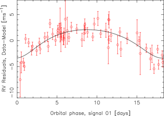
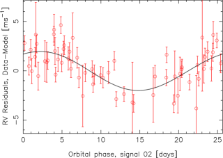
Based on the Bayesian analyses of the HD41248 radial velocities, there are two significant periodicities in the data corresponding to two super-Earths or Neptune-mass planets on nearby close-in orbits (Fig. 4). In fact, their orbits are so close to one another that the 99% credibility intervals of and taking into account the uncertainty in the stellar mass are almost overlapping (Table 5) and the configuration cannot be immediately stated to be stable in the long term. However, the orbital stability is suggested by the fact that the ratio of the orbital periods is almost exactly 1.4 with a Bayesian 99% interval of [1.384, 1.407], which suggests a possible 7:5 MMR. The eccentricities of the system also show an interesting configuration with the inner planet having an eccentricity around 0.2 and the outer planet having an eccentricity close to circular. In fact, we tested if the inner planet’s eccentricity was closer to zero by changing the eccentricity prior model to favour a more circular orbit, but the eccentricity was found to be 0.22 in this case, indicating the inner planet does have some genuine measurable eccentricity given the data. If we can rule out the source of these signals as originating from stellar magnetic activity, this could be a remarkable 7:5 MMR system, and therefore we assess this possibility in 6 by analysing the stability of the system.
5 Activity Indicators
Within our Bayesian model we have taken into account any linear correlations between the radial velocities and the activity indicators (BIS, FWHM, and ), as explained in the previous section. However, not only does the presence of activity add additional noise to any individual radial velocity measurement, but it can also mimic the presence of a true Doppler induced frequency in the full timeseries of radial velocity data (e.g. Queloz et al., 2001). Therefore, it is necessary to perform a test on whatever activity indicators one has at hand, to search for periodicities that could be associated with the periodicities found in the velocities.


In Fig. 5 we show the periodograms for each of these activity indices, going from the -indices at the top, to the BIS values in the center, and finally the FWHMs at the bottom. The -indices show a strong periodogram peak at 61 days and another slightly weaker peak at 69 days which could be the rotational period of the star, or some other activity cycle. There is no significantly strong frequency peak in the BIS periodogram, however in the FWHM periodogram there is a strong peak emerging at 71 days that could be related to the same frequency detected in the -indices. If so this may back-up the hypothesis that the rotational period of this star, or a harmonic thereof, is around 70 days, or at least there is an activity cycle present at that frequency.
The inner signal in the radial velocities at 18 days appears close to a peak in the BIS periodogram at around 18 days and this could throw some doubt on the nature of the inner signal, even though it is very unlikely for two signals to appear in a radial velocity dataset entrenched so close to such a MMR, down to the level of minutes. Also the peak in the BIS periodogram is not significant, with many more stronger peaks in the data, and since we included correlations between the BIS and the radial velocities, we can be confident this is not the source of the short period signal we detect. We also note that any power in the activity indicators at a frequency that could give rise to an alias in a periodogram search for signals, will not be detected by our Bayesian analysis, since our selection must give rise to signals with amplitudes that are significantly different from zero. This also protects our method from being confused by peaks that we see in the window function. Therefore, we must conclude that the two signals we detect close to a 7:5 MMR are genuine Doppler signals, induced by the presence of two low-mass planets orbiting HD41248.
6 System Stability
The HD41248 system poses an interesting dynamical challenge because of the proximity of the 7:5 mean-motion resonance and the close spacing of the two planets, both to each other, and to the central star. Here General Relativistic (GR) effects play a role in the dynamical stability. Before moving on to perform a numerical search for stable configurations, we list several key properties of the system that determine its stability.
Chambers (2001) defined several measures that he used to quantify a system of planets, these are: the Angular Momentum Deficit (AMD; Laskar, 1997), the fraction of total mass in the most massive planet (), a spacing parameter () that scales as the planet to star mass ratio rather than the Hill relation of (Chambers et al., 1996), and a concentration parameter () which measures how the mass is concentrated in an annulus. We supplement this with the measure stating the average spacing in Hill radii (). The values of these quantities for Venus and Earth, Jupiter and Saturn and HD41248 are listed in Table 6.
| System | AMD | ||||
|---|---|---|---|---|---|
| VE | 8 | 0.554 | 17.5 | 204.5 | 26.2 |
| JS | 1.6 | 0.769 | 8.3 | 80.3 | 7.9 |
| HD41248 | 3.4 | 0.560 | 6.9 | 411.0 | 8.5 |
As one may see, the AMD of HD41248 is nearly twice as high as that of Jupiter and Saturn, and much higher than that of Venus and Earth. Systems with higher AMD have the possibility to be more chaotic (Laskar, 1997) and have more opportunity to exchange it among the planets. The relatively high AMD of HD41248 and the fact that one planet appears much more eccentric than the other suggests that both eccentricities will fluctuate with a large amplitude, with one planet being at a minimum (c) when the other is at a maximum (b).
Given that both planets have a nearly equal mass it is no surprise that . More interesting is the spacing parameter. This quantity is only 7 while for Venus and Earth it is about 18. Even for Jupiter and Saturn it is slightly larger. However, it is interesting to see how scales as a function of the masses of the planets. We have where is the mutual Hill radius i.e. . This can be solved for to give
| (2) |
where . Setting and yields , but when inserting the masses of Jupiter and Saturn one has . Thus, even though Jupiter and Saturn have a similar spacing than HD41248 in terms of their mutual Hill radii, they are spaced father apart in relative semi-major axis ratio than the HD41248 system, implying that Jupiter and Saturn need a higher eccentricity to begin crossing their orbits than the planets of HD41248. Indeed, for HD41248 the orbits begin to cross when both planets have an eccentricity near 0.1, so unless they are apsidally aligned or protected by a resonance, they will become unstable. The nominal eccentricity of planet b is near 0.1, so the system is close to instability and the stability may crucially depend on their phasing.
In Fig. 6 we have plotted the secular evolution of both planets using the nominal orbital elements. The value of is unconstrained so we set i.e. the difference in the argument of periastron, to 20∘. The right panel shows the evolution of planet b in the eccentricity- plane while the right panel shows the same for planet c. The planets are in apsidal alignment i.e. librates around 0 and both planets show substantial excursions in their eccentricity amplitude. This alignment prevents many close encounters. We did not find the resonant angles to librate for this simulation. The question is whether this motion persists for all initial conditions allowed by the observations. Numerical simulations should shed light on this issue.

6.1 Numerical methods
We proceeded to perform a large number ( 40 000) of short simulations of the HD41248 system, which were then analysed for stability and or chaos.
We performed grid searches of both planets in the and planes. The stability dependence upon the mutual inclination was not tested. At this stage the dependence on the masses was not tested either because of the large possible range depending on the orientation of the system with respect to the observer. However, an estimate of the stability dependence on the masses can be made and maximum masses can be computed as follows.
For a planet on a fairly eccentric orbit, the chaotic boundary surrounding this planet is given by (Mustill & Wyatt, 2012)
| (3) |
This differs from the law of Wisdom (1980) since it takes eccentricity into account. Taking both planets as 10 M⊕ and setting their eccentricities we have . The planets are spaced 0.035 AU apart and thus , suggesting the system could be stable. Chaotic instability would set in when , which can be solved and yields . Taking implies that the masses need to exceed 60 M⊕, well outside the uncertainties.
We are dealing with two planets on planar orbits, so that we have four degrees of freedom: the semi-major axis or period ratio, the eccentricities and . We performed a grid search for all of these parameters.
The first grid search was done in the semi-major axis-argument of periastron plane of planet b, keeping all other orbital elements at their nominal values. The inclination and longitude of the ascending node were set to zero. For planet c Fig. 3 shows that is almost arbitrary, so we set it to 0 for the sake of simplicity. We varied evenly in steps of 3∘ between 0 and 360∘ and sampled assuming a Gaussian distribution with mean and standard deviation given in Fig. 3 using 99 steps. This resulted in 11880 simulations. The sampling method employed here takes into account the density distribution of the semi-major axis but does not consider mutual correlations between the elements.
The planets were integrated for 20 500 yr using the SWIFT MVS integrator (Levison & Duncan, 1994). We included the effects of GR by adding the potential term , where is the speed of light (Nobili & Will, 1986). This term reproduces the general relativistic effect of Mercury’s perihelion advancement. For all simulations the time step was set to 210-4 yr and output was every 10 yr.
We analyse the stability of the system using frequency analysis (Laskar, 1993). The basic method is as follows: using a numerical integration of the orbit over a time interval of length , we compute a refined determination of the semi-major axes , obtained over two consecutive time intervals of length . The stability index provides a measure of the chaotic diffusion of the trajectory. Low values close to zero correspond to a regular solution, while high values are synonymous with strong chaotic motion (Laskar). The advantage of the frequency analysis method is that it does not require long-term simulations and thus large regions of phase space can be tested with a reasonable amount of CPU power (Correia et al., 2005).
A similar methodology was employed for the other three sets of simulations. The eccentricities were sampled according to the best-fit distributions and we set .
6.2 Results
In this section we present the results from the numerical simulations determining the stable regions. These results will be presented in a series of figures.
Fig. 7 displays the stability index of the system as a function of the period ratio and . For this figure we varied the value of within its observed range. The axis labels indicate the quantity that was varied while the colour coding shows D. Motion where is considered chaotic and possible instability may occur (Correia et al., 2005).
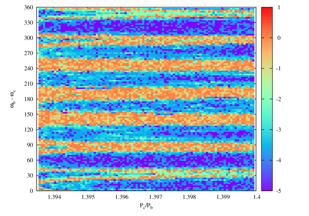
An interesting feature are the seven horizontal regions of strong chaos and instability that appear independent of period ratio but occur at regular intervals as varies. We verified that in these regions the motion is unstable: the planets encounter each other on short time scales. Varying and results in essentially the same outcome as that displayed in Fig. 7. The structure at low and low period ratio marks the limits of the 7:5 resonance.
The reason for these regions of unstable motion have to do with the proximity of the 7:5 resonance. Without the resonance the system would only have a single degree of freedom, , and thus be integrable (Michtchenko & Malhotra, 2004). The integrable system may exhibit one of three types of motion: librates around 0 (apsidal alignment), circulates and librates around (apsidal anti-alignment; see Morbidelli et al. (2009) for a discussion on these three types of motion). Without the presence of the resonance increasing the initial value of from 0 to 360∘ results in the system displaying all three types of motion in three distinct regions.
It should be noted that regions surrounding the period ratio of these planets are clustered with potential MMRs. Nearby and stronger first-order MMRs are the 3:2 and 4:3 commensurabilities, the similar strength 6:4 and 8:6 second-order MMRs around found around this dynamical region, and so are the weaker 10:7 and 11:8 third-order MMRs. Therefore, we ran some tests to ensure the 7:5 MMR is the most likely dynamical configuration for this system, given the orbital parameters. Taking the periods and uncertainties from Table 5, and assuming Gaussian distributions for each, we computed the distribution of the period ratio (/) and found a mean and of 1.397 and 0.003, respectively. The narrow range of periods given by the orbital elements constrains the possible MMR to be only the 7:5 ratio, since even the nearest 10:7 and 11:8 MMRs are found to be 8 and 6 away, respectively.
From the analysis of the motion of we find that the system most likely has librating around 0 because this configuration yields all stable solutions. When circulates or librates around the system is chaotic, and often unstable.
However, the presence of the resonance changes the system’s behaviour. The 7:5 is second order, and thus there are three resonant arguments:
| (4) | |||||
where is the mean longitude and and is the mean anomaly. The system is planar and thus is undefined (we set it to zero). The proximity of the resonance causes the seven maxima and minima in as a function as it circulates or librates around 180∘.
We have decided to display this evolution in a series of figures. Starting from the bottom-right corner of Fig. 7 the system becomes unstable when so a transition must occur. We displayed the evolution in the (left column) and planes (right column) for three simulations in Fig. 8. The top panels depict the evolution while the motion is still regular, the middle panels show the motion at the edge of the instability strip, and the bottom panels show the motion for an unstable configuration (although we only depicted the motion until the instability occurred).

In the top panels both planets have librate around 0. Increasing the initial value of from the top panels to the middle panels one sees a fundamental change in the middle-left panel. There appear to be two regions of motion: one in which librates around 0 and one in which it circulates. The motion starts as libration around 0 with mean eccentricity 0.08 and small amplitude (small loop on the right) but the system encounters a saddle and can librate around 0 with large amplitude changes of the eccentricity. The full motion is libration of around 0 but it encompasses two separate regions. However, every once in a while the separatrix is crossed and also circulates. This suggests the system is on the edge of a resonance. The motion for planet c has also changed: previously it showed a single loop but now it encompasses a moon-shaped region that is typical for libration in a resonance (e.g. Murray & Dermott, 1999). In the lowest panels circulates because the planets have crossed the separatrix. The apsidal no longer prevents them from encounters and the system is unstable.
We searched our solutions for libration of the angles but we found no case where these angles librated. We checked this by calculating the resonant angles for each simulation and tabulating the mean, minimum and maximum values. If libration occurs then the minima and maxima should be different from 0 and 360 and the mean should be zero or 180. However, in each case we always found the minima and maxima to be 0 and 360, and the mean to be close to 180, suggesting that the angles circulate. We have inspected a large sample by eye and conclude that we did not witness any libration occurring. While this procedure should break down for unstable cases, configurations which are stable for the entire simulation duration should have their minima and maxima confined to a small range. We believe this could be caused by the influence of GR, which primarily affects the pericentre precession of close-in planets. In turn, this can help break or support a resonant configuration and also affect the stability of multi-planet systems (e.g. Veras & Ford, 2010).

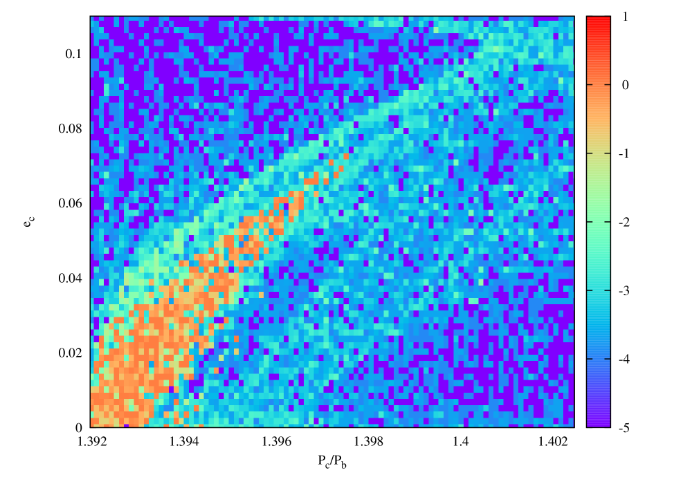
The stability dependence of the system on the eccentricities of both planets is displayed in Figs. 9 and 10. For these simulations we set the initial value of so that we would not witness any instability related to this quantity. We varied and for Fig. 9 and and for Fig. 10. As one may see, the system is mostly stable as a function of and unless , apart from some regions at low period ratio. For such high values of the apsidal alignment does not protect the planets from encounters because the orbit of planet b already crosses that of planet c, regardless of the eccentricity of planet c. There is some fine structure visible in the figure of which the line going from (1.3955,0.08) to (1.4,0.03) is the most interesting. Below this line there is a large region of stable motion and here circulates. However the eccentricities are small enough that the planets do not cross their orbits and they are protected by the 7:5 resonance. Above this region the stability is guaranteed by the apsidal alignment (apart from at high eccentricity).
In Fig. 10 we see a large unstable region at low eccentricity and low period ratio. Here the planets are at the edge of the resonance which results in chaotic motion and large excursions in eccentricity resulting in encounters. The stable region on the right has the motion being dominated by small eccentricity and by the resonance so there are few encounters, while at high eccentricity and low period ratio the planets are not in resonance but the apsidal alignment prevents close encounters.
In summary, a system of two super-Earth planets is most likely in the HD41248 data when one considers the nominal orbits, provided that the apses are nearly aligned. Given that appears unconstrained by observations, this configuration is a viable outcome. The apsidal alignment provides protection against close encounters at high and low eccentricities, as long as the eccentricities are of comparable value. If the eccentricity of one planet exceeds 0.2 while the other is nearly zero, the system becomes unstable. However, such extreme configurations can be ruled out by the observational uncertainties.
7 Discussion
The population of low-mass exoplanets tends to differ significantly from that of more massive planets. Observational evidence for a lack of low-mass planets orbiting the most metal-rich stars (Jenkins et al., 2013) points to fundamentally different evolutionary properties between low and high mass planets. As discussed in the introduction, there also appears to be a higher fraction of dynamically packed low-mass planetary systems with planets close to MMR’s.
Here we report the discovery of a possible 7:5 MMR planetary system, consisting of two super-Earths orbiting a metal-poor star. Alone this discovery adds to the number of metal-poor stars with low-mass planets and lends more weight to the hypothesis presented in Jenkins et al. It could also be the first confirmed super-Earth system of planets in such a second-order resonant configuration since libration of the longitude of periastrons yield a highly stabilized system, and our data set and simulations leave the possibility for libration of the resonant angles, and hence resonance. Also the Doppler data period ratio differs from the true 7:5 period ratio by less than 1 part in 300, a strong argument in favour of the MMR.
Around 1/3rd of multi-planet systems discovered by radial velocities are found to be close to a MMR (Lissauer et al., 2011) but the fraction actually in the resonance is significantly lower. However, Lissauer et al. show that the number of known systems in a MMR is significantly more than that expected from a randomly drawn population. Predictions from convergent migration show that around 1% of resonant systems should last for around a disk lifetime (Adams et al., 2008) whereas planet-planet scattering mechanisms yield MMRs around 5-10% of the time (Raymond et al., 2008). If we take the Kepler resonant numbers from Lissauer et al. at face value, since the number of false positives from multi-transiting systems is expected to be significantly lower than that from single transiting events (Latham et al., 2011), then we might expect that the HD41248 planetary system was formed through the planet-planet scattering mechanism. However, it may not be so straight-forward.
Terquem & Papaloizou (2007) studied the migration of cores through a proto-planetary disk that includes mutual interactions between the cores and found that the presence of MMRs is common. They found that simulations that began with a larger outer planetary distribution radius, or that started with significantly lower core masses, would tend to produce the 7:5 MMR. This indicates that such a second-order MMR that forms in this way requires longer timescales, since reducing the core masses or increasing the planetary core distance from the star gives rise to a longer evolutionary time, and thus if the HD41248 planets were formed in this way we might expect they started with low initial core masses, possibly by forming late in the disk evolution, or they started life much further out in the disk than their current semi-major axes, or most likely a combination of both low core masses and long convergent migration. It is interesting to note that even though planet-planet scattering simulations produce more MMRs, the results from Raymond et al. (2008) never resulted in a 7:5 MMR commensurability.
Finally, we should note the mass ratio between these planets. HD41248 is found to be 12.3 M⊕and planet is 8.6 M⊕, giving rise to a mass ratio of 0.7. The simulations of Terquem & Papaloizou (2007) ended with much lower mass ratios for the planets that were found in the 7:5 configuration. They found mass ratios of 0.1 and 0.2, however the more massive planet was the one closer to the star, similar to the system we present here. We do note that finding MMRs that have much lower mass ratios is difficult due to the inherent difficulties of first discovering very low-amplitude signals in radial velocity datasets, and also the difficulty of finding low-amplitude multi-planet signals when the super-position of the Keplerians has a strong dominating signal and a much weaker and longer period signal. With this in mind, we expect more of these systems to emerge from the radial velocity data with the addition of more Doppler data and better analysis techniques.
References
- Adams et al. (2008) Adams, F. C., Laughlin, G., & Bloch, A. M. 2008, ApJ, 683, 1117
- Anglada-Escudé et al. (2012) Anglada-Escudé, G., Arriagada, P., Vogt, S. S., et al. 2012, ApJL, 751, L16
- Anglada-Escudé & Butler (2012) Anglada-Escudé, G. & Butler, R. P. 2012, ApJS, 200, 15
- Anglada-Escudé & Tuomi (2012) Anglada-Escudé, G. & Tuomi, M. 2012, A&A, 548, A58
- Baluev (2013) Baluev, R. V. 2013, MNRAS, 429, 2052
- Buchhave et al. (2012) Buchhave, L. A., Latham, D. W., Johansen, A., et al. 2012, Nature, 486, 375
- Casagrande et al. (2011) Casagrande, L., Schönrich, R., Asplund, M., et al. 2011, A&A, 530, A138
- Chambers (2001) Chambers, J. E. 2001, Icarus, 152, 205
- Chambers et al. (1996) Chambers, J. E., Wetherill, G. W., & Boss, A. P. 1996, Icarus, 119, 261
- Correia et al. (2005) Correia, A. C. M., Udry, S., Mayor, M., et al. 2005, A&A, 440, 751
- Desort et al. (2008) Desort, M., Lagrange, A.-M., Galland, F., et al. 2008, A&A, 491, 883
- Fabrycky et al. (2012) Fabrycky, D. C., Ford, E. B., Steffen, J. H., et al. 2012, ApJ, 750, 114
- Fischer & Valenti (2005) Fischer, D. A. & Valenti, J. 2005, ApJ, 622, 1102
- Gomes et al. (2005) Gomes, R., Levison, H. F., Tsiganis, K., & Morbidelli, A. 2005, Nature, 435, 466
- Haario et al. (2001) Haario, H., Saksman, E., & Tamminen, J. 2001, Bernoulli, 7, 223
- Ivanyuk et al. (2013) Ivanyuk, O., Jenkins, J., Pavlenko, Y., Jones, H., & Pinfield, D. 2013, MNRAS, in prep
- Jenkins et al. (2008) Jenkins, J. S., Jones, H. R. A., Pavlenko, Y., et al. 2008, A&A, 485, 571
- Jenkins et al. (2006) Jenkins, J. S., Jones, H. R. A., Tinney, C. G., et al. 2006, MNRAS, 372, 163
- Jenkins et al. (2013) Jenkins, J. S., Jones, H. R. A., Tuomi, M., et al. 2013, ApJ, 766, 67
- Jenkins et al. (2011) Jenkins, J. S., Murgas, F., Rojo, P., et al. 2011, A&A, 531, A8
- Laskar (1993) Laskar, J. 1993, Celestial Mechanics and Dynamical Astronomy, 56, 191
- Laskar (1997) Laskar, J. 1997, A&A, 317, L75
- Laskar & Correia (2009) Laskar, J. & Correia, A. C. M. 2009, A&A, 496, L5
- Latham et al. (2011) Latham, D. W., Rowe, J. F., Quinn, S. N., et al. 2011, ApJL, 732, L24
- Levison & Duncan (1994) Levison, H. F. & Duncan, M. J. 1994, Icarus, 108, 18
- Lissauer et al. (2011) Lissauer, J. J., Ragozzine, D., Fabrycky, D. C., et al. 2011, ApJS, 197, 8
- Marcy et al. (2001) Marcy, G. W., Butler, R. P., Fischer, D., et al. 2001, ApJ, 556, 296
- Michtchenko & Ferraz-Mello (2001) Michtchenko, T. A. & Ferraz-Mello, S. 2001, AJ, 122, 474
- Michtchenko & Malhotra (2004) Michtchenko, T. A. & Malhotra, R. 2004, Icarus, 168, 237
- Morbidelli et al. (2009) Morbidelli, A., Brasser, R., Tsiganis, K., Gomes, R., & Levison, H. F. 2009, A&A, 507, 1041
- Morbidelli et al. (2005) Morbidelli, A., Levison, H. F., Tsiganis, K., & Gomes, R. 2005, Nature, 435, 462
- Murray & Dermott (1999) Murray, C. D. & Dermott, S. F. 1999, Solar system dynamics
- Mustill & Wyatt (2012) Mustill, A. J. & Wyatt, M. C. 2012, MNRAS, 419, 3074
- Nobili & Will (1986) Nobili, A. M. & Will, C. M. 1986, Nature, 320, 39
- Pavlenko et al. (2012) Pavlenko, Y. V., Jenkins, J. S., Jones, H. R. A., Ivanyuk, O., & Pinfield, D. J. 2012, MNRAS, 2643
- Peale (1976) Peale, S. J. 1976, ARA&A, 14, 215
- Perryman et al. (1997) Perryman, M. A. C., Lindegren, L., Kovalevsky, J., & et al. 1997, A&A, 323, L49
- Queloz et al. (2001) Queloz, D., Henry, G. W., Sivan, J. P., et al. 2001, A&A, 379, 279
- Raymond et al. (2008) Raymond, S. N., Barnes, R., Armitage, P. J., & Gorelick, N. 2008, ApJL, 687, L107
- Rivera et al. (2010) Rivera, E. J., Laughlin, G., Butler, R. P., et al. 2010, ApJ, 719, 890
- Santos et al. (2010) Santos, N. C., Gomes da Silva, J., Lovis, C., & Melo, C. 2010, A&A, 511, A54
- Sousa et al. (2011) Sousa, S. G., Santos, N. C., Israelian, G., Mayor, M., & Udry, S. 2011, A&A, 533, A141
- Terquem & Papaloizou (2007) Terquem, C. & Papaloizou, J. C. B. 2007, ApJ, 654, 1110
- Tsiganis et al. (2005) Tsiganis, K., Gomes, R., Morbidelli, A., & Levison, H. F. 2005, Nature, 435, 459
- Tuomi (2011) Tuomi, M. 2011, A&A, 528, L5
- Tuomi (2012) Tuomi, M. 2012, A&A, 543, A52
- Tuomi et al. (2013a) Tuomi, M., Anglada-Escudé, G., Gerlach, E., et al. 2013a, A&A, 549, A48
- Tuomi & Jenkins (2012) Tuomi, M. & Jenkins, J. S. 2012, ArXiv e-prints
- Tuomi & Jones (2012) Tuomi, M. & Jones, H. R. A. 2012, A&A, 544, A116
- Tuomi et al. (2013b) Tuomi, M., Jones, H. R. A., Jenkins, J. S., et al. 2013b, A&A, 551, A79
- van Leeuwen (2007) van Leeuwen, F. 2007, A&A, 474, 653
- Veras & Ford (2010) Veras, D. & Ford, E. B. 2010, ApJ, 715, 803
- Wisdom (1980) Wisdom, J. 1980, AJ, 85, 1122