NP-Hardness of Speed Scaling with a Sleep State

Abstract

A modern processor can dynamically set it’s speed while it’s active, and can make a transition to sleep state when required. When the processor is operating at a speed $s$, the energy consumed per unit time is given by a convex power function $P(s)$ having the property that $P(0)>0$ and $P^{\prime\prime}(s)>0$ for all values of $s$. Moreover, $C>0$ units of energy is required to make a transition from the sleep state to the active state. The jobs are specified by their arrival time, deadline and the processing volume.

We consider a scheduling problem, called speed scaling with sleep state, where each job has to be scheduled within their arrival time and deadline, and the goal is to minimize the total energy consumption required to process these jobs. Albers et. al. [1] proved the NP-hardness of this problem by reducing an instance of an NP-hard partition problem to an instance of this scheduling problem. The instance of this scheduling problem consists of the arrival time, the deadline and the processing volume for each of the jobs, in addition to $P$ and $C$. Since $P$ and $C$ depend on the instance of the partition problem, this proof of the NP-hardness of the speed scaling with sleep state problem doesn’t remain valid when $P$ and $C$ are fixed. In this paper, we prove that the speed scaling with sleep state problem remains NP-hard for any fixed positive number $C$ and convex $P$ satisfying $P(0)>0$ and $P^{\prime\prime}(s)>0$ for all values of $s$.

Keywords: Energy efficient algorithm, scheduling algorithm, NP-hardness

1 Introduction

A modern processor can dynamically set it’s speed while it’s active, and can make a transition to sleep state when required. When the processor is operating at a speed $s$, the energy consumed per unit time is given by a convex power function $P(s)$ having the property that $P(0)>0$ and $P^{\prime\prime}(s)>0$ for all values of $s$. Therefore, some energy is consumed even if the processor is not scheduling any job in the active state. On the other hand, no energy is consumed when the processor is in the sleep state. However, $C>0$ units of energy is required to make a transition from the sleep state to the active state and therefore it is not always fruitful to go asleep when there is no work to be processed at some point of time. We assume that no energy is required to make a transition from the active state to the sleep state, as we can always include this energy requirement in the sleep to active state transition. A number of problems have been studied under this model, e.g., [1], [2], [3], [4], [5], [6], [7], [8], [9], [10], [11].

The jobs are specified by their arrival time, deadline and the processing volume. We consider a scheduling problem where each job has to be scheduled within their arrival time and deadline, and the goal is to minimize the total energy consumption required to process these jobs. Albers et. al. [1] proved the NP-hardness of this problem by reducing an instance of an NP-hard partition problem (defined below) to an instance of this scheduling problem. The instance of this scheduling problem consists of the arrival time, the deadline and the processing volume for each of the jobs, in addition to $P(s)$ and $C$ that depends on the problem instance of the partition problem. As a result, this proof of NP-hardness doesn’t remain valid when we are given any fixed convex function $P(s)$ and a positive number $C$. In this paper, we prove that the problem remains NP-hard for any fixed positive number $C$ and convex function $P$ satisfying $P(0)>0$ and $P^{\prime\prime}(s)>0$ for all values of $s$.

We would do the reduction from the following NP-hard partition problem: Given a finite set $A$ of $n$ positive integers $a_{1},a_{2},\ldots,a_{n}$, the problem is to decide whether there exists a subset $A^{\prime}\subset A$ such that $\sum_{a_{i}\in A^{\prime}}a_{i}=\sum_{a_{i}\notin A^{\prime}}a_{i}$. It’s assumed that $a_{max}\geq 2$; otherwise, the problem becomes trivial.

2 The Reduction and it’s Properties

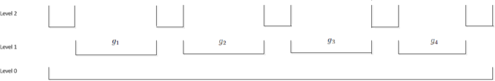
Figure 1: An instance of $I_{S}$ with $n=4$

Let us start with a few definitions and notations. The density of an interval is defined as the total workload of the jobs that completely lie in an interval divided by the length of the interval. The critical speed $s*$ for $P(s)$ is defined as the minimum speed that minimizes $\frac{P(s)}{s}$. Note that the critical speed is not well-defined if $\frac{P(s)}{s}$ decreases monotonically. However, this is not a realistic case as this would mean we can schedule all jobs at an infinite speed to get the schedule that requires the minimum amount of energy consumption. Therefore, we assume that $\frac{P(s)}{s}$ decreases for $s<s*$ and attains the minimum at $s=s*$. Under this assumption, the following property can be easily observed easily.

Lemma 1

$P^{\prime}(s)<\frac{P(s)}{s}<\frac{P(s*)}{s*}$ for $s<s*$ and $P^{\prime}(s*)=\frac{P(s*)}{s*}$.

Proof

The derivative of the function $\frac{P(s)}{s}$ is $\frac{sP^{\prime}(s)-P(s)}{s^{2}}$. Since $\frac{P(s)}{s}$ decreases for $s<s*$, we have $\frac{sP^{\prime}(s)-P(s)}{s^{2}}\leq 0$ for $s\leq s*$ with equality only when $s=s*$. $\Box$

Given the function $P(s)$, a non-negative number $C$, and an instance $I_{p}$ of the partition problem, i.e., the integers $a_{1},a_{2},\ldots,a_{n}$, let’s define the parameters which would be used to construct an instance $I_{S}$ of the scheduling problem.

$R(s)=P(s)-\frac{P(s*)}{s*}s$.

$L_{i}=e-fa_{i}$ where $e=C/R(d),d=(1-\epsilon)s*,0<\epsilon<1/2$, and $f=\frac{C}{P(0)a_{max}}$.

$l_{i}=dL_{i}-\frac{a_{i}}{k}$ where $k=\frac{-R^{\prime}(d)}{fR(d)}$.

$B=\frac{\sum\limits_{i=1}^{n}a_{i}}{2k}$.

The structure of $I_{S}$ is the same as the one used by Albers et. al. [1]. The job set in $I_{S}$ is partitioned into three levels. In level $0$, there is only one job having a processing volume equal to $B$. Level $1$ comprises of $n$ jobs; the $i$-th job has a processing volume $l_{i}$ and $L_{i}$ time units to process it. There are $n+1$ jobs in level $2$, with each job having a processing volume of $\delta s*$ and $\delta>0$ time units to process it, thereby making the density of each of these jobs equal to $s*$.

In the rest of this section, we establish a few lemmas that would be useful in our proof of NP-hardness.

Lemma 2

$R(d)<\epsilon P(0)$.

Proof

Since $R(s)=P(s)-\frac{P(s*)}{s*}s$, we obtain $R^{\prime}(s)=P^{\prime}(s)-\frac{P(s*)}{s*}$. We also note that $R(0)=P(0)>0$ and $R(s*)=0$. Furthermore, we obtain from Lemma 1 that $R^{\prime}(s*)=P^{\prime}(s*)-\frac{P(s*)}{s*}=0$, and $R^{\prime}(s)=P^{\prime}(s)-\frac{P(s*)}{s*}<0$ for $s<s*$.

Along with the properties established above, $R^{\prime\prime}(s)=P^{\prime\prime}(s)>0$ implies that the following relationship holds.

$$R(d)<(1-\frac{d}{s*})R(0)+\frac{d}{s*}R(s*)\Rightarrow R(d)<\epsilon P(0).$$

$\Box$

Lemma 3

$\frac{R(d)}{|R^{\prime}(d)|}<\epsilon s*.$

Proof

It can be easily seen from Figure 2 that $|R^{\prime}(d)|>$ $\frac{R(d)}{s*-d}$ $=$ slope of line $ab$. Since $d=(1-\epsilon)s*$, it follows that $\frac{R(d)}{|R^{\prime}(d)|}<\epsilon s*$. $\Box$

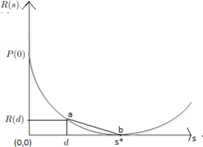
Figure 2: Plot of $s$ vs $R(s)$

We would now show that our choices of $l_{i}$ and $L_{i}$ satisfy the trivial constraints $l_{i},L_{i}>0$. We would also that the density of all the intervals except those corresponding to level $2$ jobs are strictly less than $s*$.

Lemma 4

$L_{i},l_{i}>0$ for all $i$.

Proof

We first prove that $L_{i}>0$ for all $i$. Note that

$$L_{i}>0\Leftrightarrow e-fa_{i}>0\Leftrightarrow e>fa_{i}.$$

Since $a_{max}>a_{i}$, it suffices to show that $e>fa_{max}$. As shown below, it can be easily seen using Lemma 2, $C>0$ and $0<\epsilon<\frac{1}{2}$.

$$e>fa_{max}\Leftrightarrow\frac{C}{R(d)}>\frac{C}{P(0)}\Leftrightarrow R(d)<P(0).$$

In order to show that $l_{i}>0$, we observe that

$$l_{i}>0\Leftrightarrow dL_{i}>\frac{a_{i}}{k}\Leftrightarrow d(e-fa_{i})>\frac{a_{i}}{k}\Leftrightarrow d>\frac{a_{i}}{k(e-fa_{i})}\Leftrightarrow d>\frac{1}{k(\frac{e}{a_{i}}-f)}.$$

Since $a_{max}>a_{i}$, it suffices to show that $d>\frac{1}{k\left(\frac{e}{a_{max}}-f\right)}$. We show it below using Lemma 2 and Lemma 3.

$$\frac{1}{k\left(\frac{e}{a_{max}}-f\right)} = \frac{fR(d)}{|R^{\prime}(d)|(\frac{C}{R(d)a_{max}}-f)}$$

$$= \frac{R(d)}{|R^{\prime}(d)|(\frac{C}{fR(d)a_{max}}-1)}$$

$$= \frac{R(d)R^{\prime}(d)}{|R^{\prime}(d)|(P(0)-R(d))}$$

$$= \frac{R(d)}{|R^{\prime}(d)|}\cdot\frac{1}{(\frac{P(0)}{R(d)}-1)}$$

$$< \epsilon s*(\frac{1}{\frac{1}{\epsilon}-1})$$

$$= \frac{\epsilon^{2}s*}{1-\epsilon}$$

$$< (1-\epsilon)s*=d.$$

Note that the last inequality follows from our choice of $0<\epsilon<\frac{1}{2}$. $\Box$

Figure 3: Plot of $x$ vs $G(x)$

Lemma 5

The density of all the intervals except those corresponding to level $2$ jobs are strictly less than $s*$.

Proof

Let’s first consider the intervals corresponding to level $1$ jobs. The density of such an interval is $\frac{l_{i}}{L_{i}}$. Observe that

$$\frac{l_{i}}{L_{i}}<s*\Leftrightarrow\frac{dL_{i}-\frac{a_{i}}{k}}{L_{i}}>s*\Leftrightarrow d<s*+\frac{a_{i}}{kL_{i}}.$$

Since $d<s*$, the density of an interval corresponding to a Level $1$ job is strictly less than $s*$. This also proves that the density of any interval corresponding to the union of a proper subset of the level $1$ and level $2$ jobs is less than $s*$, since such jobs are non-overlapping and the density of any interval corresponding a level $2$ job is exactly $s*$.

Finally, we consider the interval that starts from the first arrival of the level $0$ job and lasts till it’s deadline. The density of this interval is $\frac{(n+1)\delta s*+B+\sum_{i}l_{i}}{(n+1)\delta+\sum_{i}L_{i}}$. This quantity is less than $s*$ since

$$\frac{B+\sum_{i}l_{i}}{\sum_{i}L_{i}}<s*\Leftrightarrow\frac{\sum_{i}a_{i}}{2k}+d\sum_{i}L_{i}-\sum_{i}\frac{a_{i}}{k}<s*\sum_{i}L_{i}\Leftrightarrow d<s*+\frac{\sum_{i}a_{i}}{2k\sum_{i}L_{i}}.$$

The last inequality is true since $d<s*$. $\Box$

Let us introduce the functions $F(x)=\frac{P(s*)}{s*}x+C$ and $H_{i}(x)=P(\frac{x}{L_{i}})L_{i}$, and establish some of their properties.

Lemma 6

$F(x)$ and $H_{i}(x)$ intersect at two different points for any $i$.

Proof

Consider $G(x)=H_{i}(x)-F(x)=P(\frac{x}{L_{i}})L_{i}-\frac{P(s*)}{s*}x-C$. Note that

$$G(0) = P(0)L_{i}-C$$

$$= P(0)(e-fa_{i})-C$$

$$= P(0)(\frac{C}{R(d)}-\frac{Ca_{i}}{P(0)a_{max}})-C$$

$$\geq P(0)(\frac{C}{R(d)}-\frac{C}{P(0)})-C$$

$$= \frac{C(P(0)-R(d))}{R(d)}-C$$

$$> C(\frac{P(0)(1-\epsilon)}{\epsilon P(0)})-C$$

$$= C(\frac{1-2\epsilon}{\epsilon})$$

$$> 0.$$

The last-but-one inequality follows from Lemma 2. The last inequality follows since $0<\epsilon<1/2$.

Next, we would show that $G(x)$ decreases for $x<L_{i}s*$, attains minimum at $x=L_{i}s*$ and then finally increases. Note that $G^{\prime}(x)=L_{i}P^{\prime}(\frac{x}{L_{i}})\frac{1}{L_{i}}-\frac{P(s*)}{s*}=P^{\prime}(\frac{x}{L_{i}})-\frac{P(s*)}{s*}$. The following inequalities follow easily from Lemma 1 and from the fact that $P^{\prime\prime}(s)>0$.

$$G^{\prime}(x)\leq 0\Leftrightarrow P^{\prime}(\frac{x}{L_{i}})\leq\frac{P(s*)}{s*}\Leftrightarrow P^{\prime}(\frac{x}{L_{i}})\leq P^{\prime}(s*)\Leftrightarrow x\leq L_{i}s*.$$

By Lemma 1, the inequalities above would be strict since $x<L_{i}s*$.

We complete the proof by showing that $G(L_{i}s*)=P(s*)L_{i}-P(s*)L_{i}-C=-C<0$. Since $G$ is a strictly convex function (note that $G^{\prime\prime}(x)=\frac{1}{L_{i}}P^{\prime\prime}(\frac{x}{L_{i}})$), it would eventually intersects the $x$-axis at some point $x>L_{i}s*$. $\Box$

Lemma 7

$H^{\prime}_{i}(l_{i}+\frac{a_{i}}{k})=\frac{H_{i}(l_{i}+\frac{a_{i}}{k})-F(l_{i})}{a_{i}/k}=P^{\prime}(d)$.

Proof

It can be easily seen that $H^{\prime}_{i}(l_{i}+\frac{a_{i}}{k})=H^{\prime}_{i}(dL_{i})=P^{\prime}(\frac{dL_{i}}{L_{i}})=P^{\prime}(d)$. The following calculation also shows that $\frac{H_{i}(l_{i}+\frac{a_{i}}{k})-F(l_{i})}{a_{i}/k}=P^{\prime}(d)$.

$$\frac{H_{i}(l_{i}+\frac{a_{i}}{k})-F(l_{i})}{a_{i}/k} = \frac{k}{a_{i}}[H_{i}(dL_{i})-F(l_{i})]$$

$$= \frac{k}{a_{i}}[P(d)L_{i}-\frac{P(s*)}{s*}l_{i}-C]$$

$$= \frac{k}{a_{i}}[P(d)L_{i}-\frac{P(s*)}{s*}dL_{i}+\frac{P(s*)}{s*}\frac{a_{i}}{k}-C]$$

$$= \frac{k}{a_{i}}R(d)L_{i}+\frac{P(s*)}{s*}-\frac{Ck}{a_{i}}$$

$$= \frac{k}{a_{i}}R(d)e-\frac{k}{a_{i}}R(d)fa_{i}+\frac{P(s*)}{s*}-\frac{Ck}{a_{i}}$$

$$= \frac{k}{a_{i}}C+R^{\prime}(d)+\frac{P(s*)}{s*}-\frac{Ck}{a_{i}}$$

$$= P^{\prime}(d)-\frac{P(s*)}{s*}+\frac{P(s*)}{s*}$$

$$= P^{\prime}(d).$$

$\Box$

Let $r_{i1}$ and $r_{i2}$ be the two roots of the equation $F(x)=H_{i}(x)$ such that $r_{i1}<r_{i2}$. We establish the following two lemmas.

Lemma 8

$0<l_{i}<r_{i1}$, where $r_{i1}$ is the first intersection of $H_{i}(x)$ and $F(x)$.

Proof

Since $H_{i}(x)$ is strictly convex at every $x$, we obtain

$$H^{\prime}_{i}(l_{i}+\frac{a_{i}}{k})>\frac{H_{i}(l_{i}+\frac{a_{i}}{k})-H_{i}(l_{i})}{a_{i}/k} \Rightarrow \frac{H_{i}(l_{i}+\frac{a_{i}}{k})-F(l_{i})}{a_{i}/k}>\frac{H_{i}(l_{i}+\frac{a_{i}}{k})-H_{i}(l_{i})}{a_{i}/k}$$

$$\Rightarrow -F(l_{i})>-H_{i}(l_{i})$$

$$\Rightarrow G(l_{i})>0.$$

The lemma follows since $l_{i}<L_{i}s*$. $\Box$

Lemma 9

$r_{i1}<(l_{i}+\frac{a_{i}}{k})<r_{i2}$.

Proof

Assume for the sake of contradiction that $l_{i}+\frac{a_{i}}{k}\leq r_{i1}$. It can be seen from Figure 4 that it implies $\frac{H_{i}(l_{i}+\frac{a_{i}}{k})-F(l_{i})}{a_{i}/k}\geq\frac{P(s*)}{s*}$ $\Rightarrow P^{\prime}(d)\geq\frac{P(s*)}{s*}$. However, this leads to a contradiction since $d<s*$, and $P^{\prime}(d)<\frac{P(s*)}{s*}$ by Lemma 1. On the other hand, it’s easy to see that $l_{i}+\frac{a_{i}}{k}=dL_{i}<L_{i}s*<r_{i2}$ . $\Box$

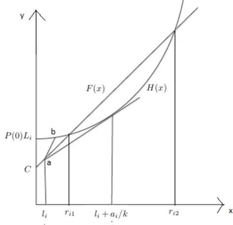
Figure 4: Plot of $x$ vs $F(x)$ and $H(x)$

3 Proof of NP-hardness

In this section, we would complete the proof of the NP-hardness of the speed scaling with power down problem. We would be using the following result by Irani et al. [9] along with the results derived in the previous section.

Lemma 10

[9] There exists an optimal solution of the “speed scaling with a sleep state” problem that satisfies the following properties:

• A job $j$ must be scheduled at a constant speed $s_{j}.$
  

• Suppose that the arrival time and the deadline of a job $j$ is $r_{j}$ and $d_{j}$, respectively. If another job $k$ is scheduled in the interval $[r_{j},d_{j}]$, then $s_{k}\geq s_{j}$.
  

• The jobs in the intervals having density at least $s*$ are scheduled according to the YDS algorithm [11]. The YDS algorithm is an iterative algorithm. In each iteration, an interval with the maximum density is identified and an earliest-deadline-first policy is used to construct a schedule for the jobs that lie completely in that interval. After an iteration, the YDS algorithm removes the jobs that lie completely in the maximum density interval corresponding to that iteration, and updates the arrival time and deadline of any job that overlaps with that interval.

Theorem 3.1

An instance $I_{p}$ of the partition problem admits a partition if and only if there exists a a feasible schedule for $I_{s}$ with total energy consumption of at most $(n+1)\delta P(s*)+\sum\limits_{i=1}^{n}F(l_{i})+BP^{\prime}(d)$.

Proof

$(\Rightarrow)$ Let’s first assume that $I_{p}$ admits a partition and construct a feasible schedule of energy at most $(n+1)\epsilon P(s*)+\sum\limits_{i=1}^{n}F(l_{i})+BR_{min}$. We start with some notations.

Let $A^{\prime}$ be the set of i corresponding to the solution of Partition problem, i.e., $\sum\limits_{i\in A^{\prime}}a_{i}=\frac{\sum\limits_{i=1}^{n}a_{i}}{2}$. Let $b_{i}$ denote the portion of the workload of Level 0 job scheduled in gap $g_{i}$. It can be seen that $\sum\limits_{i=1}^{n}b_{i}=B$. We set the $b_{i}$’s as follows:

$b_{i}=\left\{\begin{array}[]{r l}a_{i}/k,&\mbox{if }i\in A^{\prime}\\ 0,&\mbox{otherwise}.\end{array}\right.$

Our schedule executes any Level $2$ jobs with speed $s*$ between it’s release time and deadline. This is feasible since the density of any such job is equal to $s*$. Therefore, a total workload of $l_{i}+a_{i}/k=dL_{i}$ has to be scheduled in each gap $g_{i}$ corresponding to an $i\in A^{\prime}$. We schedule both the jobs in gap $g_{i}$ with speed $d$. In the rest of the gaps, the Level $1$ jobs are scheduled at speed $s*$. The processor transitions to the sleep state at the completion of the job in such gaps, and wakes up at the release time of a Level $2$ job. Since the density of any interval corresponding to a Level $1$ job is less than $s*$, we get a feasible schedule.

Let us calculate the total energy consumed by the jobs at every level. First of all, the total energy consumed by the Level 2 jobs is $(n+1)\delta P(s*)$. In the gaps corresponding to $i\in A^{\prime}$, we note that the jobs are proceeded at a speed $d=(\frac{l_{i}+a_{i}/k}{L_{i}})$ for $L_{i}$ units of time. The energy consumption in such a gap equals $P(\frac{l_{i}+a_{i}/k}{L_{i}})L_{i}$, which is the same as $H_{i}(l_{i}+\frac{a_{i}}{k})$. In a gap corresponding to $i\notin A^{\prime}$, a total $l_{i}$ units of workload are scheduled at speed $s*$ and then the processor transitions to sleep state. Therefore, the energy consumed is given by $P(s*)\frac{l_{i}}{s*}+C$, which is the same as $F(l_{i})$. From lemma 7, $H_{i}(l_{i}+\frac{a_{i}}{k})$ can be written as $F(l_{i})+P^{\prime}(d)\frac{a_{i}}{k}$.

Let $E_{0,1}$ denote the total Energy consumed by the Level $0$ and Level $1$ jobs. We obtain the following.

$$E_{0,1} = \sum\limits_{i\in A^{\prime}}H_{i}(l_{i}+\frac{a_{i}}{k})+\sum\limits_{i\notin A^{\prime}}F(l_{i})$$

$$= \sum\limits_{i\in A^{\prime}}(F(l_{i})+P^{\prime}(d)\frac{a_{i}}{k})+\sum\limits_{i\notin A^{\prime}}F_{i}(l_{i})$$

$$= \sum\limits_{i=1}^{n}F(l_{i})+P^{\prime}(d)\sum\limits_{i\in A^{\prime}}\frac{a_{i}}{k}$$

$$= \sum\limits_{i=1}^{n}F(l_{i})+P^{\prime}(d)B.$$

The last equality follows since $\sum\limits_{i=1}^{n}b_{i}=\sum\limits_{i\in A^{\prime}}a_{i}/k=(\sum\limits_{i=1}^{n}a_{i})/2k=B$. Hence, we get a feasible schedule whose total energy consumption is $(n+1)\delta P(s*)+\sum\limits_{i=1}^{n}F(l_{i})+P^{\prime}(d)B$.

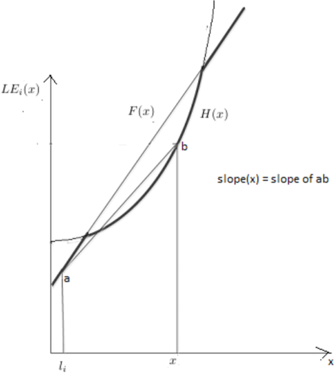
Figure 5: Plot of $x$ vs the lower envelope function $LE_{i}(x)$

($\Leftarrow$) In the reverse direction of the proof, we assume that $I_{p}$ doesn’t admits a partition and show that the energy consumption in any feasible schedule is strictly greater than $(n+1)\delta P(s*)+\sum\limits_{i=1}^{n}F(l_{i})+BP^{\prime}(d)$.

Let $LE_{i}(x)=min\{F(x),H_{i}(x)\}$ denote the lower envelope of the functions $F(x)$ and $H_{i}(x)$, represented by solid curve in Figure 5. Let slope(x) denote the slope of the line joining $(l_{i},LE_{i}(l_{i}))$ and $(x,LE_{i}(x))$. For $x\geq l_{i}$, $LE_{i}(x)$ can be written as $LE_{i}(x)=LE_{i}(l_{i})+(LE_{i}(x)-LE_{i}(l_{i}))=F(l_{i})+(slope(x))*(x-l_{i})$. We note that the slope(x) is minimum at $x=l_{i}+\frac{a_{i}}{k}$ and the minimum value is $H^{\prime}(l_{i}+\frac{a_{i}}{k})=P^{\prime}(d)$ (by Lemma 7) which is independent of $i$.

Consider an Optimal schedule $S$ satisfying the properties of lemma 10 and let $b_{1},b_{2},....,b_{n}$ units of workload of Level 0 job be scheduled in the gaps $g_{1},g_{2},.....,g_{n}$, respectively. Let $A^{\prime}=\{i|r_{i1}\leq l_{i}+b_{i}\leq r_{i2}\}$.

Case 1. $b_{i}=\frac{a_{i}}{k}$ for some $i\in A^{\prime}$

Since the workload $l_{i}+b_{i}$ is greater than $r_{i1}$ and less than $r_{i2}$, it is beneficial to schedule it at the speed $(l_{i}+b_{i})/L_{i}$ (rather than to schedule it with the speed $s*$) and then transition to sleep state. From Lemma 10, it follows that the ratio $(l_{i}+b_{i})/L_{i}$ must be the same for all $i\in A^{\prime}$ in the schedule $S$. Take $i\in A^{\prime}$ corresponding to $b_{i}=\frac{a_{i}}{k}$. We show below that $b_{j}$ must also be equal to $a_{j}/k$ for all $j\in A^{\prime}$ in an optimal schedule.

$$\frac{(b_{i}+l_{i})}{L_{i}}=\frac{(b_{j}+l_{j})}{L_{j}} \Rightarrow \frac{a_{i}/k+dL_{i}-a_{i}/k}{L_{i}}=\frac{b_{j}+dL_{j}-a_{j}/k}{L_{j}}$$

$$\Rightarrow d=d+\frac{b_{j}-a_{j}/k}{L_{j}}$$

$$\Rightarrow b_{j}=a_{j}/k.$$

Lemma 10 says that all the intervals having density greater than or equal to s* must be scheduled according to YDS in the schedule $S$. Also, Lemma 1 tells that all the intervals except those corresponding to Level 2 jobs are having density less than s*. Therefore, in the schedule $S$, all Level 2 jobs must be scheduled at s*. Thus, the total energy consumed by the Level 2 jobs is $(n+1)\delta P(s*)$.

Let us again denote the total energy required by the Level 0 and level 1 jobs as $E_{0,1}$. In a gap corresponding to $i\notin A^{\prime}$, it is optimal to schedule the job at speed $s*$ and then transition to sleep state than scheduling at the speed $(l_{i}+b_{i})/L_{i}$. When this is feasible, the energy consumption in the gap would be given by $LE(l_{i}+b_{i})$. When it’s not (i.e., if $(l_{i}+b_{i})/L_{i}>s*$), the energy consumption in the gap would be greater than $LE_{i}(l_{i}+b_{i})$. Therefore, we obtain the following lower bound on $E_{0,1}$.

$$E_{0,1} \geq\sum\limits_{i\in A^{\prime}}LE_{i}(l_{i}+\frac{a_{i}}{k})+\sum\limits_{i\notin A^{\prime}}LE_{i}(l_{i}+b_{i})$$

$$=\sum\limits_{i\in A^{\prime}}(F(l_{i})+P^{\prime}(d)\frac{a_{i}}{k})+\sum\limits_{i\notin A^{\prime}}(F(l_{i})+\frac{P(s*)}{s*}b_{i})$$

$$=\sum\limits_{i=1}^{n}F(l_{i})+P^{\prime}(d)\sum\limits_{i\in A^{\prime}}a_{i}/k+\frac{P(s*)}{s*}(B-\sum\limits_{i\in A^{\prime}}b_{i}).$$

If $\sum\limits_{i\in A^{\prime}}b_{i}=B$, it implies that $\sum\limits_{i\in A^{\prime}}\frac{a_{i}}{k}=\frac{\sum\limits_{i=1}^{n}a_{i}}{2k}$, which contradicts our assumption that a solution of the partition problem does not exist. Therefore, $\sum\limits_{i\in A^{\prime}}b_{i}<B$, which implies that $\sum\limits_{i\in A^{\prime}}a_{i}/k<B$. The following calculation completes the proof of Case $1$.

$$E_{0,1} \geq\sum\limits_{i=1}^{n}F(l_{i})+P^{\prime}(d)\sum\limits_{i\in A^{\prime}}a_{i}/k+\frac{P(s*)}{s*}(B-\sum\limits_{i\in A^{\prime}}a_{i}/k)$$

$$=\sum\limits_{i=1}^{n}F(l_{i})+B\frac{P(s*)}{s*}-(\sum\limits_{i\in A^{\prime}}a_{i}/k)(\frac{P(s*)}{s*}-P^{\prime}(d))$$

$$>\sum\limits_{i=1}^{n}F(l_{i})+B\frac{P(s*)}{s*}-B(\frac{P(s*)}{s*}-P^{\prime}(d))$$

$$=\sum\limits_{i=1}^{n}F(l_{i})+BP^{\prime}(d)$$

Case 2. $b_{i}\neq a_{i}/k$ for all $i\in A^{\prime}$

In this case, the following calculation completes the proof.

$$E_{0,1} =\sum\limits_{i\in A^{\prime}}(F(l_{i})+slope(l_{i}+b_{i})*b_{i})+\sum\limits_{i\notin A^{\prime}}(F(l_{i})+slope(l_{i}+b_{i})*b_{i})$$

$$>\sum\limits_{i\in A^{\prime}}F(l_{i})+P^{\prime}(d)\sum\limits_{i\in A^{\prime}}b_{i}+\sum\limits_{i\notin A^{\prime}}F(l_{i})+P^{\prime}(d)\sum\limits_{i\notin A^{\prime}}b_{i}$$

$$=\sum\limits_{i=1}^{n}F(l_{i})+BP^{\prime}(d).$$

$\Box$

References

- [1] S. Albers and A. Antoniadis. Race to Idle: New algorithms for speed scaling with a sleep state. Proceedings of the 23rd Annual ACM-SIAM Symposium on Discrete Algorithms, 1266-1285, 2012.
- [2] E. Bampis, C. Dürr, F. Kacem and I. Milis. Speed scaling with power down scheduling for agreeable deadlines (submitted).
- [3] P. Baptiste. Scheduling Unit Tasks to Minimize the Number of Idle Periods: A Polynomial Time Algorithm for Offline Dynamic Power Management. Proc. 17th Annual ACM-SIAM Symposium on Discrete Algorithms, 364-367, 2006.
- [4] P. Baptiste, M. Chrobak and C. D¨urr. Polynomial time Algorithms for Minimum Energy Scheduling. Proc. 15th Annual European Symposium on Algorithms, 136-150, 2007.
- [5] N. Bansal, H. L. Chan, T. W. Lam and K. L. Lee. Scheduling for speed bounded processors. Proc. 35th International Colloquium on Automata, Languages and Programming, 409-420, 2008.
- [6] N. Bansal, H. L. Chan, K. Pruhs and D. Katz. Improved bounds for speed scaling in devices obeying the cube-root rule. Proc. 36th International Colloqium on Automata, Languages and Programming, 144-155, 2009.
- [7] H. L. Chan, W. T. Chan, T. W. Lam, K. L. Lee, K. S. Mak and P. W. H. Wong. Optimizing throughput and energy in online deadline scheduling. ACM Transactions on Algorithms 6, 2009.
- [8] X. Han, T. W. Lam, L. K. Lee, I. K. K. To and P. W. H. Wong. Deadline scheduling and power management for speed bounded processors. Theoretical Computer Science 411: 3587-3600, 2010.
- [9] S. Irani, S.K. Shukla and R. Gupta. Algorithms for power savings. ACM Transactions on Algorithms 3, 2007.
- [10] S. Irani and K. Pruhs. Algorithmic Problems in Power Management. SIGACT News, 36:63-76, 2005.
- [11] F.F. Yao, A.J. Demers and S. Shenker. A scheduling model for reduced CPU energy. Proc. 36th IEEE Symposium on Foundations of Computer Science, 374-382, 1995.