Asymptotic FRESH Properizer for Block Processing of Improper-Complex Second-Order Cyclostationary Random Processes
Abstract
In this paper, the block processing of a discrete-time (DT) improper-complex second-order cyclostationary (SOCS) random process is considered. In particular, it is of interest to find a pre-processing operation that enables computationally efficient near-optimal post-processing. An invertible linear-conjugate linear (LCL) operator named the DT FREquency Shift (FRESH) properizer is first proposed. It is shown that the DT FRESH properizer converts a DT improper-complex SOCS random process input to an equivalent DT proper-complex SOCS random process output by utilizing the information only about the cycle period of the input. An invertible LCL block processing operator named the asymptotic FRESH properizer is then proposed that mimics the operation of the DT FRESH properizer but processes a finite number of consecutive samples of a DT improper-complex SOCS random process. It is shown that the output of the asymptotic FRESH properizer is not proper but asymptotically proper and that its frequency-domain covariance matrix converges to a highly-structured block matrix with diagonal blocks as the block size tends to infinity. Two representative estimation and detection problems are presented to demonstrate that asymptotically optimal low-complexity post-processors can be easily designed by exploiting these asymptotic second-order properties of the output of the asymptotic FRESH properizer.
Index Terms:
Asymptotic analysis, complexity reduction, improper-complex random process, properization, second-order cyclostationarityI Introduction
It is well known that the complex envelope of a real-valued bandpass wide-sense stationary (WSS) random process is proper, i.e., its complementary auto-covariance (a.k.a. the pseudo-covariance) function vanishes [1]. However, there are a lot of important improper-complex random processes that do not have vanishing complementary auto-covariance functions [2, 3, 4]. For example, the complex envelope of a real-valued bandpass nonstationary signal is not necessarily proper and even the complex envelope of a real-valued bandpass WSS signal becomes improper in the presence of the imbalance between its in-phase and quadrature components [5]. In order to fully capture the statistical properties of a complex-valued signal, including all the second-order statistics, the filtering of augmented signals has been proposed. This so-called widely linear (WL) filtering processes either the signal augmented by its complex conjugate or the real part of the signal augmented by the imaginary part [6, 5], where the former is referred to as the linear-conjugate linear (LCL) filtering [7].
On the other hand, many digitally modulated signals are well modeled by wide-sense cyclostationary (WSCS) random processes [8, 9], whose complex envelopes possess periodicity in all variables of the mean and the auto-covariance functions. To efficiently extract the correlation structure of a WSCS random process in the time and the frequency domains, the translation series representation (TSR) and the harmonic series representation (HSR) are proposed [10], which are linear periodically time-varying (PTV) processings. Using these representations, it is shown [10] that a proper-complex WSCS scalar random process can be converted to an equivalent proper-complex WSS vector random process. Such second-order structure of a proper-complex WSCS random process has long been exploited in the design of many communications and signal processing systems including presence detectors [11, 12], estimators [13, 14, 15], and optimal transceivers [16, 17, 18] under various criteria.
The complex envelopes of the majority of digitally modulated signals are proper and WSCS. However, as well documented in [5], there still remain many other digitally modulated signals such as pulse amplitude modulation (PAM), offset quaternary phase-shift keying (OQPSK), and Gaussian minimum shift keying (GMSK), that are not only improper-complex WSCS but also second-order cyclostationary (SOCS) [19], i.e., the complementary auto-covariance function is also periodic in all its variables with the same period as the mean and the auto-covariance functions. To exploit both cyclostationarity and impropriety, the LCL FREquency Shift (FRESH) filter has been proposed in [20] that combines signal augmentation and linear PTV processing.
Recently, another LCL PTV operator called the properizing FRESH (p-FRESH) vectorizer is proposed in [19, 21] by non-trivially extending the HSR. The p-FRESH vectorizer converts an improper-complex SOCS scalar random process to an equivalent proper-complex WSS vector random process by exploiting the frequency-domain correlation and complementary correlation structures that are rigorously examined in [3]. By successfully deriving the capacity of an SOCS Gaussian noise channel, it is shown that the optimal channel input is improper-complex SOCS in general when the interfering signal is improper-complex SOCS. It is also well demonstrated that such properization provides the advantage of enabling the adoption of the conventional signal processing techniques and algorithms that utilize only the correlation but not the complementary correlation structure. These results warrant further research in communications and signal processing on the efficient construction and processing of improper-complex SOCS random processes.
In this paper, we consider the block processing of a complex-valued random vector that is obtained by taking a finite number of consecutive samples from a discrete-time (DT) improper-complex SOCS random process. To proceed, the p-FRESH vectorization developed for continuous-time (CT) SOCS random processes is first extended to DT improper-complex SOCS random processes. Instead of straightforwardly modifying the CT p-FRESH vectorizer that properizes as well as vectorizes the input CT improper-complex SOCS random process, an invertible LCL operator is proposed in this paper that does not vectorize but only properizes the input DT improper-complex SOCS random process. Thus, the LCL operator is named the DT FRESH properizer and its output does not need vector processing. Specifically, the DT FRESH properizer transforms a DT improper-complex SOCS scalar random process into an equivalent proper-complex SOCS scalar random process with the cycle period that is twice the cycle period of the input process.
To make this idea of pre-processing by properization better suited for digital signal processing, an invertible LCL block processing operator is then proposed that mimics the operation of the DT FRESH properizer. Although the augmentation of the improper-complex random vector by its complex conjugate can generate a sufficient statistic [5], it is not only a redundant information of twice the length of the original observation vector but also improper. Although the strong uncorrelating transform (SUT) of the observation vector can generate a highly-structured sufficient statistic of the same length as the original observation vector [5, 22], the output is still improper and, moreover, it requires the information about both the correlation and the complementary correlation matrices of the improper-complex random vector input for the transformation. Thus, neither the augmenting pre-processor nor the SUT allows the direct application of the conventional techniques and algorithms dedicated to the block processing of proper-complex random vectors. Motivated by how the DT FRESH properizer works in the frequency domain, the pre-processor proposed in this paper utilizes the centered discrete Fourier transform (DFT) and the information only about the cycle period of the DT improper-complex SOCS random process in order to convert a finite number of consecutive samples of the random process to an equivalent random vector. Unlike the output of the DT FRESH properizer, the output of this LCL block processing operator is not proper but approximately proper for sufficiently large block size. Thus, the pre-processor is named the asymptotic FRESH properizer. Specifically, the asymptotic FRESH properizer makes the sequence of the complementary covariance matrices of the output asymptotically equivalent [23] to the sequence of all-zero matrices.
In [24], it is shown that the complex-valued random vector consisting of a finite number of consecutive samples of a DT proper-complex SOCS random process has its frequency-domain covariance matrix that approaches a block matrix with diagonal blocks as the number of samples increases. This is because the periodicity in the second-order statistics of the DT SOCS random process naturally leads to a sequence of block Toeplitz covariance matrices as the number of samples increases, the sequence of block Toeplitz matrices is asymptotically equivalent to a sequence of block circulant matrices, and a block circulant matrix becomes a block matrix with diagonal blocks when pre- and post-multiplied by DFT and inverse DFT matrices, respectively. Since the asymptotic FRESH properizer mimics the DT FRESH properizer and the DT FRESH properizer outputs a DT proper-complex SOCS random process, it naturally becomes of interest to examine the asymptotic property of the frequency-domain covariance matrix of the asymptotic FRESH properizer output. It turns out that the output of the asymptotic FRESH properizer has the same property discovered in [24].
Such properties of the covariance and the complementary covariance matrices may be used in designing, under various optimality criteria, low-complexity post-processors that follow the asymptotic FRESH properizer. In particular, a post-processor can be developed that approximates the output of the asymptotic FRESH properizer by a proper-complex random vector having the block matrix with diagonal blocks that is asymptotically equivalent to the exact frequency-domain covariance matrix as its frequency-domain covariance matrix. Of course, this technique makes the post-processor suboptimal that performs most of the main operations in the frequency domain. As the two asymptotic properties strongly suggest, however, if the block size is large enough, then the performance degradation may be negligible. It is already shown in [24] that this is the case for the asymptotic property only of the covariance matrix, where a suboptimal frequency-domain equalizer is proposed that approximates the frequency-domain covariance matrix of a proper-complex SOCS interference by an asymptotically equivalent block matrix with diagonal blocks. It turns out that this equalizer not only achieves significantly lower computational complexity than the exact linear minimum mean-square error (LMMSE) equalizer by exploiting the block structure of the frequency-domain covariance matrix, but also is asymptotically optimal in the sense that its average mean-squared error (MSE) approaches that of the LMMSE equalizer as the number of samples tends to infinity.
To demonstrate the simultaneous achievability of asymptotic optimality and low complexity by employing the post-processor that processes the output of the asymptotic FRESH properizer and exploits the two asymptotic properties, we consider two representative estimation and detection problems. First, for a DT improper-complex SOCS random signal in additive proper-complex white noise, a low-complexity signal estimator is proposed that is a linear function of the output of the asymptotic FRESH properizer. It is shown that the average MSE performance of the estimator approaches that of the widely linear minimum mean-squared error (WLMMSE) estimator as the number of samples tends to infinity. Second, for a DT improper-complex SOCS Gaussian random signal in additive proper-complex white Gaussian noise, a low-complexity signal presence detector is proposed whose test statistic is a quadratic function of the output of the asymptotic FRESH properizer It is shown that the test statistic converges to the exact likelihood ratio test (LRT) statistic that is a quadratic function of the augmented observation vector with probability one (w.p. ) as the number of samples tends to infinity. Note that in both cases the asymptotic FRESH properizer as the pre-processor utilizes only the information about the cycle period. Thus, the adoption of adaptive estimation and detection algorithms may be possible that are developed for the processing of proper-complex random vectors. This advantage of employing the asymptotic FRESH properizer may be taken in other communications and signal processing problems involving the block processing of DT improper-complex SOCS random processes.
The rest of this paper is organized as follows. In Section II, definitions and lemmas related to SOCS random processes are provided and the DT FRESH properizer is proposed. In Section III, the asymptotic FRESH properizer is proposed and the second-order properties of its output are analyzed. In Sections IV and V, the application of the asymptotic FRESH properizer is considered to exemplary estimation and detection problems, respectively. Finally, concluding remarks are offered in Section VI.
Throughout this paper, the operator denotes the expectation, the operator denotes the discrete-time Fourier transform (DTFT) of an absolutely summa-ble sequence , and the function denotes the Dirac delta function. The sets and are the sets of all integers and of all positive integers, respectively. The operator denotes the Cartesian product between two sets. The superscripts ∗, T, and H denote the complex conjugation, the transpose, and the Hermitian transpose, respectively. The operator denotes the convolution.111There should be no confusion from the superscript ∗ that denotes the complex conjugation. The operators and denote the Hadamard product and the Kronecker product, respectively. The matrices , , , and denote the -by- all-one matrix, the -by- identity matrix, the -by- all-zero matrix, and the -by- all-zero matrix, respectively. The matrix denotes the -by- backward identity matrix whose th entry is given by for , and otherwise. The operator and denote the th entry and the trace of a matrix , respectively. To describe the computational complexity, we will use the big-O notation defined as if and only if there exist a positive constant and a real number such that .
II DT FRESH Properizer
In this section, the notion of DT second-order cyclostationarity is introduced and an LCL PTV operator is proposed that converts a DT improper-complex SOCS random process into an equivalent DT proper-complex SOCS random process. Similar to the p-FRESH vectorizer proposed in [19], where an input CT SOCS random process is converted to an equivalent CT proper-complex WSS vector random process, this operator as a pre-processor enables the adoption of the conventional signal processing techniques and algorithms that utilize only the correlation but not the complementary correlation structure of the signal. Note that, unlike the p-FRESH vectorizer, this DT operator does not vectorize but only properizes the input improper-complex SOCS random process. A CT version of this properizer can be found in [25].
II-A DT SOCS Random Processes
In this subsection, definitions and lemmas related to the DT SOCS random processes are provided.
Definition 1
Given a DT complex-valued random process with a finite power, i.e., , the mean, the auto-correlation, the auto-covariance, the complementary auto-correlation, and the complementary auto-covariance functions of are defined, respectively, as
| (1a) | |||||
| (2a) | |||||
| (3a) | |||||
| (4a) | |||||
| (5a) |
Throughout this paper, all DT complex-valued random processes are assumed to be of finite power, i.e., .
Definition 2
The two-dimensional (2-D) power spectral density (PSD) and the 2-D complementary PSD of a DT complex-valued random process are defined as
| (6a) | |||||
| (7a) | |||||
respectively, if they exist.
Since the 2-D PSD and the 2-D complementary PSD are the DT double Fourier transforms of and , respectively, they are always periodic in both variables and with the common period . The set of all DT complex-valued random processes can be partitioned into two subsets by using the following definition.
Definition 3
[1, Definition 2] A DT complex-valued random process is proper if its complementary auto-covariance function vanishes, i.e., and is improper otherwise.
Two types of stationarity can be defined as follows by using the second-order moments of a DT complex-valued random process.
Definition 4
[26, Section II-B] A DT complex-valued random process is second-order stationary (SOS) if,
| (8a) | |||||
| (9a) | |||||
| (10a) |
Definition 5
A DT complex-valued random process is SOCS with cycle period if,
| (11a) | |||||
| (12a) | |||||
| (13a) |
We are mainly interested in the DT SOCS random processes in this paper. Note that a DT SOS random process can be viewed as a special DT SOCS random process with cycle period . Note also that the above definition of a DT SOCS random process is a straightforward extension of the definition of a CT SOCS random process in [19]. For the ease of comparison with the results in [19], we use the time indexes and in the orders appearing in Definitions 1-5.
In the following lemmas, the implications of the second-order cyclostationarity are provided in the time and the frequency domains, respectively.
Lemma 1
For a DT SOCS random process with cycle period , there exist and such that
| (14a) | |||||
| (15a) | |||||
Proof:
Lemma 2
For a DT SOCS random process with cycle period , the 2-D PSD and the 2-D complementary PSD are given, respectively, by
where and .
Proof:
II-B DT FRESH Properizer
In this subsection, an LCL PTV operator is proposed that always outputs an equivalent DT proper-complex random process, regardless of the propriety of the input DT SOCS random process. In what follows, all SOCS random processes are DT processes unless otherwise specified.
To proceed, the following frequency-selective filter is defined that has half of the entire frequency band as its stopband.
Definition 6
Given a reference frequency , a linear time-invariant system with impulse response is called the frequency-domain raised square wave (FD-RSW) filter if its frequency response is given by
| (18) |
Fig. 1 shows the frequency response of the FD-RSW filter with reference frequency , which alternately passes the frequency components of the input signal in every other interval of bandwidth . Hereafter, denotes the support of this FD-RSW filter. By using the impulse response of the FD-RSW filter with reference frequency , we can define an LCL PTV filter as follows.
Definition 7
Given a reference frequency and an input , the DT FRESH properizer is defined as a single-input single-output LCL PTV system, whose output is given by
| (19) |
Fig. 2 shows how the DT FRESH properizer works in the time domain, where is the input, is the output, and and are, respectively, the first and the second terms on the right side of (19). Note that, unlike the upper branch where is processed by the FD-RSW filter to generate , is processed in the lower branch by the FD-RSW filter and multiplied by a complex-exponential function to generate . Even though is chosen as the frequency of the complex-exponential function, any for can be chosen. The reason why this is so becomes clear once the DT FRESH properization is viewed in the frequency domain.
Fig. 3 shows how the DT FRESH properizer works in the frequency domain, especially when the input is a deterministic signal with the DTFT , the outputs of the upper and the lower branches in Fig. 2 are denoted by with the DTFT and with the DTFT , respectively, and the output signal is denoted by with the DTFT . Note that is processed by the FD-RSW filter to generate the first term of the DTFT of the DT FRESH properizer output, while is processed by the FD-RSW filter and shifted in the frequency domain to generate the second term . Thus, contains all the frequency components of on the support of the FD-RSW filter, while contains all the remaining frequency components. Since the supports of and do not overlap, the DTFT of the output of the DT FRESH properizer contains all the frequency components of the input signal without any distortion. Note also that, due to the periodicity of the DTFT with period , the frequency shift of by any for generates the output signal that contains the same information as the input does. The following lemma makes this invertibility argument more precise.
Lemma 3
From the output of the DT FRESH properizer with reference frequency , the input of the DT FRESH properizer can be recovered as
| (20) |
Note that, at this point, the DT FRESH properizer may not be more than one of many possible invertible operators. The reason why this operator is named the properizer will become clear once the second-order property of the output is analyzed as follows when its input is a zero-mean SOCS random process.
Theorem 1
If the input to the DT FRESH properizer with reference frequency is a zero-mean SOCS random process with cycle period , then the output becomes a zero-mean proper-complex SOCS random process with cycle period , i.e., the mean, the auto-correlation, and the complementary auto-correlation functions of satisfy
| (21a) | |||||
| (22a) | |||||
| (23a) |
, respectively.
Proof:
It is straightforward to show (21a) by using . Let and be defined again as shown in Fig. 2. Then, the auto-correlation function of can be written as
| (24) |
The first term on the right side of (24) can be rewritten as
| (25a) | |||||
| (26a) |
where (25a) holds by Parseval’s relation and (26a) holds by substituting (LABEL:eq:_R_X_a) into (25a). It turns out in (26a) that is periodic in both and with period . Similarly, the second term of (24) can be rewritten as
| (27) |
It also turns out in (27) that is periodic in both and with period . In the same way, the other two terms can be obtained, which turn out to be periodic in and with period and , respectively. Thus, the auto-correlation function of satisfies (22a).
On the other hand, the complementary auto-correlation function of can be written as
| (28) |
The first and the second terms of the right side of (28) can be rewritten, respectively, as
| (29a) | |||
| and | |||
| (29b) | |||
by using Parseval’s relation. These two terms are all zeros because the impulse fences of and along the line for any do not cross the integration area . Fig. 4 illustrates these lines and the integration area. Similarly, the other two terms of can be obtained, which again turn out to be all zeros. Thus, the complementary auto-correlation function of satisfies (23a). Therefore, the conclusion follows. ∎
This theorem shows that the DT FRESH properizer in general doubles the cycle period at the cost of the propriety of the output. However, it does not double the cycle period if the input is already proper.
Corollary 1
If the input to the DT FRESH properizer with reference frequency is a zero-mean proper-complex SOCS random process with cycle period , then the output is a zero-mean proper-complex SOCS random process with cycle period .
Proof:
It suffices to show that is periodic in and with period . It is already shown in Theorem 1 that the first and the forth terms of are periodic in and with period . As it can be easily seen in (27), the second term on the right side of (24) is zero, , because the propriety of implies . Similarly, the third term is zero. Therefore, the conclusion follows. ∎
It is already shown that the amount of the frequency shift in the second term of (19) can be any , for , to satisfy the invertibility of the DT FRESH properizer. It can be also shown that Theorem 1 holds for any frequency shift , for . Moreover, since any integer multiple of is also a cycle period of an SOCS random process with cycle period , the random process can be FRESH properized by using any reference frequency . Thus, it is not unique to FRESH properize an SOCS random process.
III Asymptotic FRESH Properizer
In this section, the block processing of an SOCS random process is considered. Motivated by how the DT FRESH properizer works in the frequency domain, an LCL block operator is proposed that converts a finite number of consecutive samples of an SOCS random process to an equivalent random vector. Unlike the DT FRESH properizer proposed in the previous section, this invertible operator does not directly make the complementary covariance matrix of the output vector vanish. Instead, it is shown that the LCL operator makes the complementary covariance matrix of the output vector approach all-zero matrix as the number of samples tends to infinity. This is why it is named the asymptotic FRESH properizer.
III-A Asymptotic FRESH Properizer and Its Inverse Operator
Let be the length- vector obtained by taking the consecutive samples of a DT signal, where and in what follows it is assumed that is a positive even number. Motivated by the DT FRESH properizer, we introduce in this subsection an LCL block operator and its inverse.
To proceed, some definitions are provided.
Definition 8
The centered DFT matrix is defined as an -by- matrix whose th entry, for , is given by
| (30) |
where .
It is well known that the matrix-vector multiplication with a centered DFT matrix can be implemented with low computational complexity [27], as the multiplication with an ordinary DFT matrix is efficiently implemented by using the fast Fourier transform algorithm.
Definition 9
Given and an even number , the -by- matrix is defined as
| (31) |
Similar to the FD-RSW pulse, the matrix will be called the raised square wave (RSW) matrix because, when pre-multiplied to a column vector or a matrix, it turns the th row, for and , into all zeros, i.e., it alternately nulls every other band of consecutive rows.
Definition 10
Given and an even number , the -by- matrix is defined as
| (32) |
Note that the matrix , when pre-multiplied to a column vector or a matrix, circularly shifts the rows by , which corresponds to multiplying in the second term of the right side of (19). Now, we are ready to introduce an LCL operator that is the block-processing counterpart to the DT FRESH propertizer.
Definition 11
Given and an even number , the LCL operator with input and output , both of length , is called the asymptotic FRESH properizer if
| (33) |
Note that the input is pre-multiplied by the centered DFT matrix and the RSW matrix , while the complex conjugate is multiplied additionally by the circular shift matrix to generate the frequency-domain output .
Fig. 5 shows , , and , when the th entry of the is denoted by . Note that, similar to the DT FRESH properization illustrated in Fig. 3, the locations of all possible non-zero rows of and do not overlap, which makes contain all the entries of without any distortion. Note also that the amount of the circular shift of by any for generates the signal that contains the same information as does. The following lemma makes this invertibility argument more precise.
Lemma 4
From the output of the asymptotic FRESH properizer with parameters and , the input of the asymptotic FRESH properizer can be recovered as
| (34a) | |||||
| (35a) |
Proof:
Note that, at this point, the asymptotic FRESH properizer may not be more than one of many possible invertible operators. The reason why this operator is named the asymptotic properizer will become clear once the second-order property of the output is analyzed in the next subsection when its input is a finite number of consecutive samples of a zero-mean SOCS random process.
III-B Second-Order Properties of Output of Asymptotic FRESH Properizer
Let be the length- augmented vector defined as
| (36) |
where and in what follows it is assumed that consists of a finite number of consecutive samples of a zero-mean SOCS random process with cycle period . Then, the output in (33) of the asymptotic FRESH properizer can be rewritten as
| (37a) | |||||
| (38a) |
where the -by- matrix and the -by- matrix are given by
| (39a) | |||||
| (40a) |
respectively, and is the centered DFT of . Thus, the covariance matrix and the complementary covariance matrix of are given by
| (41a) | |||||
| (42a) | |||||
respectively, where and denote the covariance and the complementary covariance matrices of the augmented vector , respectively.
Throughout this paper, we call
| = | W_MNR_yW_MN^H | (43a) | |||||
| = | W_MN~R_yW_MN^T | (44a) | |||||
the frequency-domain covariance and the frequency-domain complementary covariance matrices, respectively.
To analyze the asymptotic second-order properties of , we briefly review definitions and related lemmas for asymptotic equivalence between two sequences of matrices.
Definition 12
[23] Let and be two sequences of -by- matrices with as . Then, and are asymptotically equivalent and denoted by if 1) the strong norms of and are uniformly bounded, i.e., there exists a constant such that , and 2) the weak norm of vanishes asymptotically, i.e., , where the strong norm and the weak norm of an -by- matrix are defined as and , respectively.
Lemma 5
If two sequences and of -by- matrices are asymptotically equivalent and if the strong norms of -by- matrices and are uniformly bounded, then .
Proof:
Since and , it is straightforward to show the conclusion by applying [23, Theorem 1-(3)] twice. ∎
Lemma 6
If and , then (.
Proof:
By applying the triangle inequality, it is straightforward to show that the strong norms of and are uniformly bounded and that the weak norm of vanishes asymptotically. Therefore, the conclusion follows. ∎
For brevity, in what follows, two square matrices and of the same size will be said to be asymptotically equivalent if . Now, we introduce our definition of asymptotic propriety.
Definition 13
A sequence of length- complex-valued random vectors is asymptotically proper if the complementary covariance matrix of is asymptotically equivalent to the -by- all-zero matrix.
For brevity, a random vector will be said to be asymptotically proper if the sequence is asymptotically proper. Before showing that the output of the asymptotic FRESH properizer is asymptotically proper, the second-order properties of the augmented vector are examined as follows.
Proposition 1
If the random vector is obtained by taking the consecutive samples from a zero-mean SOCS random process with cycle period , then the covariance matrix and the complementary covariance matrix of the augmented vector defined in (36) satisfy
| (45a) | |||||
| (46a) | |||||
respectively, where the -by- matrices and are given by
| (47a) | |||||
| (48a) | |||||
respectively.
Proof:
By definition, the left sides of (45a) and (46a) can be rewritten, respectively, as
Since both and are -by- block Toeplitz matrices with block size -by-, each submatrix on the right side of (LABEL:eq:_aug_cov) is asymptotically equivalent to the Hadamard product of and the submatrix itself as shown in [24, Proposition 1]. Thus, by using the fact that if each submatrix of is asymptotically equivalent to the corresponding submatrix of [24, Lemma 5], we obtain (45a). Similar to (45a), it can be shown by using the property of the centered DFT matrix that each submatrix on the right side of (LABEL:eq:_aug_com_cov) is asymptotically equivalent to Hadamard product of and the submatrix itself. Thus, we obtain (46a). Therefore, the conclusion follows. ∎
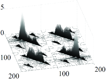
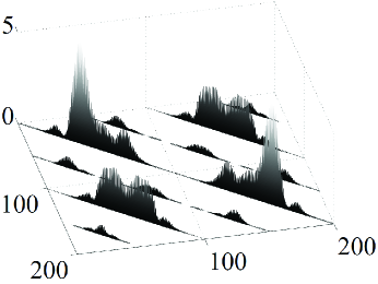
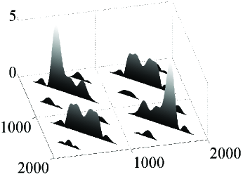
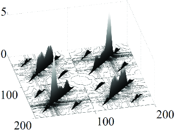
Figs. 6 and 7 show the entry-by-entry magnitudes of the exemplary frequency-domain covariance and complementary covariance matrices. To generate a zero-mean improper-complex SOCS random process, equally-likely BPSK symbols are linearly modulated with the square-root raised cosine (SRRC) pulse having roll-off factor and transmitted at the symbol rate of [symbols/sec]. After the BPSK signal passes through the frequency selective channel with impulse response , the SOCS random process is obtained by -times over-sampling the received signal, i.e., the sampling rate is [samples/sec]. Thus, the zero-mean SOCS random process has the cycle period . As shown in (45a), it can be seen in Fig. 6 that approaches as increases. Similarly, as shown in (46a), it can be seen in Fig. 7 that approaches as increases.
![[Uncaptioned image]](/html/1304.7375/assets/x4.png)
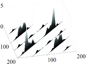
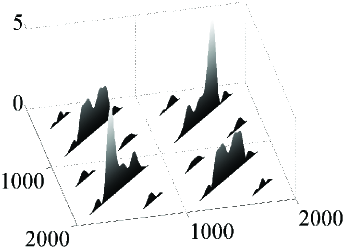
![[Uncaptioned image]](/html/1304.7375/assets/x8.png)
Now, the asymptotic second-order properties of the output of the asymptotic FRESH properizer are examined as follows.
Theorem 2
If the input to the asymptotic FRESH properizer with parameters and is obtained by taking the consecutive samples from an SOCS random process with cycle period , then the covariance and the complementary covariance matrices of the output of the asymptotic FRESH properizer satisfy
| (51a) | |||||
| (52a) | |||||
where an -by- matrix is given by
| (53a) | |||||
| (54a) |
Proof:
By Definition 13 and the above theorem, the output of the asymptotic FRESH properizer is indeed asymptotically proper. Fig. 8-(a) illustrates how the frequency-domain covariance matrix of the output of the asymptotic FRESH properizer is constructed from . The thick diagonal lines in each block of size -by- represent all possible non-zero entries of that is asymptotically equivalent to . Then, that is asymptotically equivalent to is obtained by collecting the shaded sub-blocks of size -by-. Fig. 8-(b) illustrates how the frequency-domain complementary covariance matrix of the output of the asymptotic FRESH properizer is constructed from . The thick anti-diagonal lines in each block of size -by- represent all possible non-zero entries of that is asymptotically equivalent to . Then, that is asymptotically equivalent to is obtained by collecting the shaded sub-blocks of size -by-.
It is already shown that the amount of the circular shift of in (31) can be any , for , to satisfy the invertibility of the asymptotic FRESH properizer. It can be also shown that Theorem 2 holds for every circular shift by , for . Moreover, since and that are -by- block Toeplitz matrices with block size -by- can be viewed as block Toeplitz matrices with block size -by-, , the sampled vector can be asymptotically properized by using any parameters and , for all such that is even. Thus, similar to the DT FRESH properizer, it is not unique to asymptotically properize a finite number of consecutive samples of a zero-mean SOCS random process with cycle period .
In the following two sections, two representative estimation and detection problems are presented to demonstrate that low-complexity asymptotically optimal post-processors can be easily designed by exploiting the asymptotic second-order properties of the output of the asymptotic FRESH properizer.
IV Application of Asymptotic FRESH Properizer to Signal Estimation Problem
In this section, given a finite number of consecutive samples of a zero-mean improper-complex SOCS random process in additive proper-complex white noise, the minimum mean squared error estimation of the random process is considered when only the second-order statistics of the observation vector are provided. It is well known [5] that an optimal estimator is the WLMMSE estimator that linearly processes the observation vector augmented by its complex conjugate. This optimality of the use of the augmented vector still holds even if the output of the asymptotic FRESH properizer is processed, because the output as an equivalent observation vector is still improper. Instead, motivated by Theorem 2, we propose to use the LMMSE estimator that processes the output of the asymptotic FRESH properizer as if the signal component is a proper-complex random vector with its frequency-domain covariance matrix being equal to the masked version of the exact frequency-domain covariance matrix. It turns out that this suboptimal linear estimator is asymptotically optimal in the sense that the difference of its average MSE performance from that of the WLMMSE estimator having higher computational complexity converges to zero as the number of samples tends to infinity.
IV-A Asymptotically Optimal Low-Complexity Estimator
Let be the length- observation vector modeled by
| (55) |
where is the desired signal to be estimated that consists of the consecutive samples of a zero-mean improper-complex SOCS random process with cycle period , and is the additive proper-complex white noise vector.
Given the observation model (55) and the second-order moments , , , , , and of and , the WLMMSE estimation problem can be formulated as
| (56) |
where the average MSE is defined as
| (57) |
In the following lemma, the optimal solution to the above estimation problem is provided along with its average MSE performance. It is well known [5] that the optimal estimator that minimizes the average MSE without the wide linearity constraint becomes this WLMMSE estimator if the desired signal vector and the additive noise vector are both Gaussian.
Lemma 7
The WLMMSE estimator of as the solution to the optimization problem (56) is given by
| (58) |
where
| (59a) | |||||
| (60a) | |||||
with . Moreover, the average MSE is given by
| (61) |
Proof:
See [5, Section 5.4] and the references therein. ∎
The WLMMSE estimator in (58) requires the computation of two matrices and to be pre-multiplied to and , respectively. As it can be seen from (59a) and (60a), the major burden in computing these matrices comes from the multiplications and the inversions of -by- matrices. It can be shown that the matrix multiplications in computing and require complex-valued scalar multiplications because the matrix does not have any structure to be exploited in matrix-matrix multiplications even though is block Toeplitz. By the same reason, the matrix inversion in (59a) and (60a) requires complex-valued scalar multiplications. Thus, the overall computational complexity of the WLMMSE estimator is .
An alternative observation model that is equivalent to the original one in (55) can be obtained by applying the asymptotic FRESH properization to as
| (62) |
where , , and . Since the equivalent observation vector is not proper in general, the linear processing of and is still needed for the second-order optimal estimation of . Instead, we propose to use a suboptimal linear estimator as follows, which is a function only of .
Definition 14
The proposed estimate of is defined by
| (63) |
where is given by
| (64) |
Note from (63) and (64) that is the estimate of and, consequently, that is the estimate of . Let . Then, the estimate of is obtained as (63) by applying the inverse operation to .
It can be immediately seen that is chosen to make the LMMSE estimate of when the covariance and the complementary covariance matrices of are set equal to and appearing in (51a) and (52a), respectively. This idea of using the asymptotically equivalent matrices is motivated by Theorem 2, which naturally leads to the asymptotic optimality of the proposed estimator as shown in what follows.
First, the invariance of the Euclidean norm under the asymptotic FRESH properization is shown.
Lemma 8
The input and the output of the asymptotic FRESH properizer have the same Euclidean norm, i.e., .
Proof:
Second, the average MSE of the proposed estimator is derived.
Lemma 9
The average MSE of the proposed estimator is given by
| (65) |
Proof:
The linearity of the asymptotic FRESH properizer leads to . Then, by Lemma 8, the average MSE performance can be written as . Since is unitary and , it can be shown that we have
| (66) |
It can be also shown that if and for -by- matrices and then and . Thus, the right side of (IV-A) is invariant under replacing with in (54a). Therefore, (IV-A) can be simplified to (65). ∎
Now, the asymptotic optimality of the proposed estimator is provided.
Theorem 3
The average MSE of the proposed estimator approaches that of the WLMMSE estimator as the number of samples tends to infinity in the sense that
| (67) |
Proof:
It is shown in [5, Section 5.4] that the average MSE in (61) of the WLMMSE estimator can be simplified as
| (68) |
Now, we define and introduce
| (69a) | |||||
| (70a) |
which is obtained by replacing in (68) with and by using the fact that is unitary. Note that as shown in (45a). This introduction of is motivated by the result in [24, Theorem 1], where a suboptimal estimator is proposed for the estimation of a proper-complex cyclostationary random signal and its average MSE is shown to approach that of the LMMSE estimator as the number of samples tends to infinity. Since is a covariance matrix, it is positive semidefinite, which implies that all the eigenvalues of in (68) are upper bounded by . Note that and are also positive semidefinite because in (47a) is positive semidefinite. Similarly, all the eigenvalues of in (69a) are also upper bounded by . Thus, the strong norms and are uniformly upper bounded by for any matrix size. Recall that if and , for a positive constant , then [23, Theorem 1-(4)]. Thus, we have . Recall also that if two sequences and of -by- matrices are asymptotically equivalent then [23, Corollary 1]. Thus, combined with Lemmas 5 and 6, we have . Therefore, in order to show (67), it now suffices to show .
Let be the -by- matrix that permutes the rows of the post-multiplied matrix in such a way that the th row of the post-multiplied matrix becomes the th row for and , i.e., the rows having indexes , for are grouped for each . Then, is a -by- block diagonal matrix with block size -by-, because is a -by- block matrix with diagonal blocks of block size -by-. Similarly, the -by- matrix is defined. Let and be the -by- matrix that are defined as and , respectively, where the -by- matrix permutes the rows of the post-multiplied matrix in such a way that the th row becomes the th row and that the th row becomes the th row for . Then, the definition in (53a) leads to
| (71) |
Since , , and are all permutation matrices, in (69a) can be rewritten as , which leads to because is Hermitian symmetric. Therefore, the conclusion follows. ∎
The proposed estimator requires the pre-processing of to obtain , the computation and the multiplication of , and the inverse operation on to obtain . As it can be seen from (33) and (34a), the major burden in the asymptotic FRESH properization and its inverse operation comes from the multiplications of the -by- centered DFT matrix. This can be efficiently implemented with only complex-valued scalar multiplications by using, e.g., the fast algorithm in [27]. As it can be seen from (64), the major burden in computing comes from the inversion of . The inversion of an -by- block matrix with diagonal blocks of size -by- requires complex-valued scalar multiplications [24]. Thus, this inversion of has the same order of computational complexity because is an -by- block matrix with diagonal blocks of size -by-.
Since we consider the block processing where is a fixed small number and is much larger than , the overall complexities of the WLMMSE and the proposed estimators as functions only of can be rewritten now as and , respectively. Thus, the computational complexity of the proposed estimator is much lower than that of the WLMMSE estimator. Though not major, an additional complexity reduction comes from the fact that the proposed estimator is linear that requires the computation and multiplication of one matrix instead of two matrices and , all with columns.
IV-B Numerical Results
In this subsection, numerical results are provided that show the computational efficiency and the asymptotic optimality of the proposed estimator.
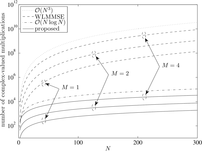
The first result is to compare the complexity of the proposed estimator with that of the WLMMSE estimator. Fig. 9 shows that the number of complex-valued multiplications needed in computing the WLMMSE and the proposed estimators for cycle periods , , and . Recall that the computational complexities of the WLMMSE and the proposed estimators are and for a fixed integer , respectively. It can be seen from Fig. 9 that the computational complexity of the proposed estimator is much lower than that of the WLMMSE estimator. As predicted, the approximation motivated by Theorem 2 leads to this significant complexity reduction.
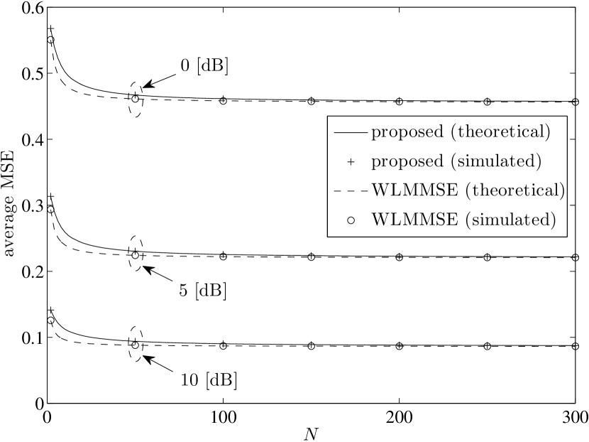
The second result is to show the asymptotic optimality of the proposed estimator. We consider the case where an improper-complex SOCS random process is obtained by uniformly sampling a CT zero-mean improper-complex SOCS random process. The CT random process is, e.g., a Gaussian jamming signal, generated by OQPSK modulating two independent real-valued independent and identically distributed zero-mean symbol sequences with the SRRC pulse having roll-off factor . This signal is sampled at -times the symbol rate of the OQPSK symbols, which results in the DT zero-mean improper-complex SOCS random process with cycle period . Thus, the entries of in (55) are the consecutive samples of the random process. Fig. 10 shows that the average MSEs of the WLMMSE and the proposed estimators versus for symbol energy per noise density , , and [dB], where the theoretical results are evaluated by (61) and (65) while the simulated results are obtained from Monte-Carlo runs. It can be seen that, as shown in Theorem 3, the average MSE of the proposed estimator approaches that of the WLMMSE estimator as increases.
V Application of Asymptotic FRESH Properizer to Signal Presence Detection Problem
In this section, again given a finite number of consecutive samples, now the signal presence presence detection of a zero-mean improper-complex SOCS Gaussian random process is considered in additive proper-complex white Gaussian noise. It is well known [28] that the likelihood ratio is a sufficient statistic for all binary hypothesis tests under any optimality criterion. In [5], it is shown that the exact LRT statistic can be written as a quadratic function of the augmented observation vector when the improper-complex random process is Gaussian. Similar to the estimation problem in the previous section, this optimality of the use of the augmented vector still holds even if the output of the asymptotic FRESH properizer as an equivalent observation vector is processed. Again motivated by Theorem 2, we propose to use this equivalent observation vector of half the length of the augmented vector as if the signal component is a proper-complex random vector with its frequency-domain covariance matrix being equal to the masked version of the exact frequency-domain covariance matrix. It turns out that this suboptimal test statistic is asymptotically optimal in the sense that its difference from the exact LRT statistic having higher computational complexity converges to zero w.p. as the number of samples tends to infinity.
V-A Asymptotically Optimal Low-Complexity Detector
Let be the length- observation vector modeled by
| v | ||||||
| (72) | ||||||
| x + v, |
where and are the null and the alternative hypotheses, respectively. The desired signal to be detected consists of the consecutive samples of a zero-mean improper-complex SOCS Gaussian random process with cycle period , and is the additive proper-complex white Gaussian noise vector.
Throughout this section, the definitions and the notations of the second-order statistics of , , and follow those in the previous section except that under the null hypothesis the second-order statistic of does not contain the desired signal component. Similar to (36), the augmented observation vector is denoted by . Then, the LRT statistic of the observation vector is provided as follows.
Lemma 10
Given the observation model (LABEL:eq:_detection_observation), the LRT statistic of is given by
| (73) |
where .
Proof:
Note that, since the length- observation vector is improper and Gaussian, the LRT statistic in (73) is a quadratic form of the length- augmented observation vector . Under any optimality criterion such as the Neyman-Pearson, the Bayesian, and the minimax criteria, the optimal detector computes , compares it with an optimal threshold , and then declares if and otherwise.
The computation of requires the matrix inversion of , which is the -by- covariance matrix of the augmented observation vector under , and the matrix-vector multiplication. The major burden in computing comes from the matrix inversion and it requires complex-valued scalar multiplications. The matrix-vector multiplication requires only complex-valued scalar multiplications. Thus, the overall computational complexity of the LRT statistic is .
An alternative observation model that is equivalent to the original one in (LABEL:eq:_detection_observation) can be obtained by applying the asymptotic FRESH properization to as
| w | ||||||
| (74) | ||||||
| y + w, |
where , , and . Since the equivalent observation vector is not proper in general, the augmentation of and is still needed to compute the exact LRT statistic of . Instead, we propose to use a suboptimal LRT statistic as follows, which is a quadratic function only of .
Definition 15
Given the observation model (LABEL:eq:_detection_problem_FRESH), the proposed test statistic of is defined by
| (75) |
where .
It can be immediately seen that can be viewed as the exact LRT statistic of when the covariance and the complementary covariance matrices of are set equal to and appearing in (51a) and (52a), respectively. Similar to the estimation problem in the previous section, this idea of using the asymptotically equivalent matrices is again motivated by Theorem 2, which naturally leads to the asymptotic equivalence of the LRT statistic in (73) and the proposed test statistic in (75).
Now, the asymptotic optimality of the proposed test statistic is provided.
Theorem 4
The proposed test statistic approaches the exact LRT statistic as the number of samples tends to infinity in the sense that
| (76) |
under and .
Proof:
We define and introduce a suboptimal test statistic
| (77) |
which is obtained by replacing in (73) with and by using the fact that is unitary. This introduction of is motivated by in (45a). Similar to the proof of Theorem 3, it can be shown that . In [30], the LRT problems are considered where the covariance matrix of a proper-complex Gaussian signal vector is either Toeplitz or block Toeplitz. It is shown under both and that a suboptimal test statistic, which is obtained by replacing the covariance matrix in the quadratic form of the LRT statistic with its asymptotically equivalent one, converges to the exact LRT statistic w.p. as the number of samples tends to infinity [30, Propositions 1 and 3]. By applying this result, we have w.p. because . Therefore, in order to show (76), it now suffices to show .
Let be the frequency-domain equivalent observation vector that is defined as . Then, by using the permutation matrices , , and that are defined in the proof of Theorem 3 in Section IV, we have
| (78) |
By using (71) and (78), we can rewrite defined in (77) as because is real-valued and (71) leads
| (79) |
Therefore, the conclusion follows. ∎
The computation of the proposed test statistic requires the pre-processing of to obtain , the matrix inversion of , and the matrix-vector multiplication to compute the quadratic form. As shown in Section IV, the asymptotic FRESH properization of the length- vector and the matrix inversion of require and complex-valued scalar multiplications, respectively. In addition, the matrix-vector multiplication requires complex-valued scalar multiplications, because is an -by- block matrix with diagonal blocks of size -by-. Since we consider the block processing where is a fixed small number and is much larger than , the overall complexity in computing the exact LRT statistic and the proposed test statistic as functions only of can be rewritten now as and , respectively. Thus, the computational complexity of the proposed test statistic is much lower than that of the exact LRT statistic.
V-B Numerical Results
In this subsection, numerical results are provided that show only the asymptotic optimality of the proposed test statistic because its computational efficiency can be similarly shown as Fig. 9. Throughout this subsection, the zero-mean improper-complex SOCS Gaussian random process to be detected is obtained by uniformly sampling the OQPSK-like signal generated in a similar way to that described in Section IV-B.
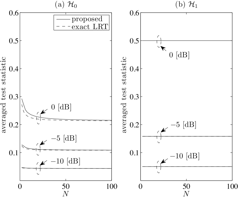
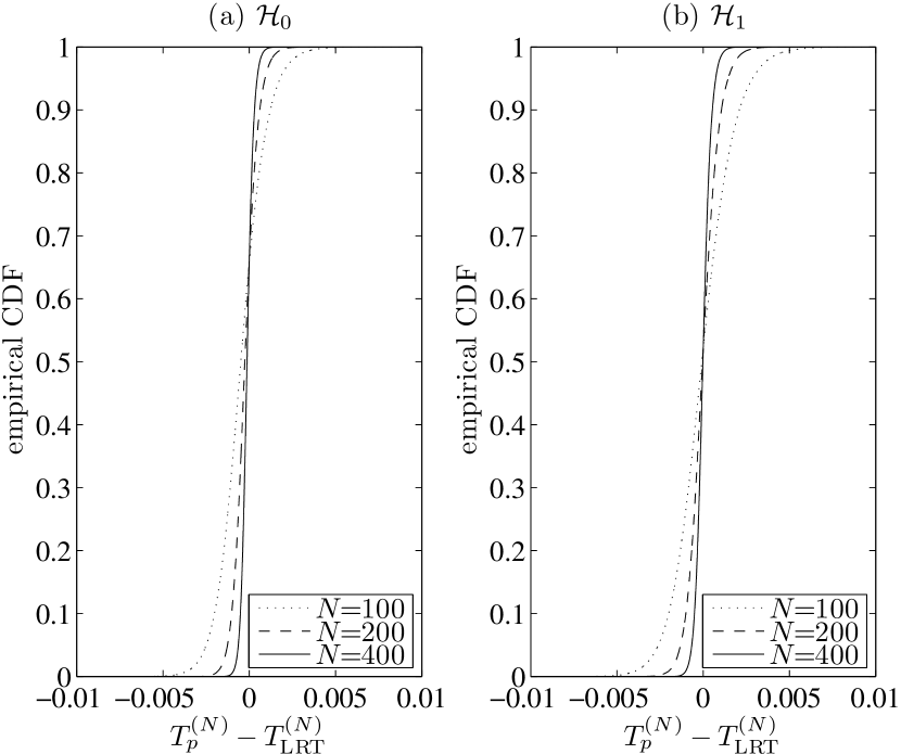
The first result is to show the convergence of the proposed test statistic to the exact LRT statistic. Fig. 11 shows the statistical average of the exact LRT and that of the proposed test statistics for symbol energy per noise density and [dB]. It can be seen that the statistical averages of the exact LRT and the proposed test statistics approach the same non-zero value as the number of samples tends to infinity under both hypotheses. In particular, they coincide under because the trace of are the same as that of . Since the convergence w.p. is hard to show by using Monte-Carlo simulations, we instead show the convergence in probability that is implied by the convergence w.p. [31]. Fig. 12 shows the empirical cumulative distribution function (CDF) of the difference of the proposed test statistic from the exact LRT statistic for symbol energy per noise density [dB] and and , where the empirical CDF is obtained by Monte-Carlo runs. It can be seen that, as implied by Theorem 4, the empirical CDF of the difference quickly converges to the unit step function as the number of samples increases under both hypotheses.
The second result is to compare the receiver operating characteristic (ROC) curves of the optimal detector that uses the exact LRT statistic (73) and the proposed detector that uses the proposed test statistic (75). As a common practice in computing the PDF of a quadratic function of Gaussian random vectors [32], we approximate the statistics by gamma random variables to obtain the probability of miss and the probability of false alarm . The CDF of the gamma random variable with two parameters and is given by
| (80) |
where the Pearson’s form of incomplete gamma function is defined by
| (81) |
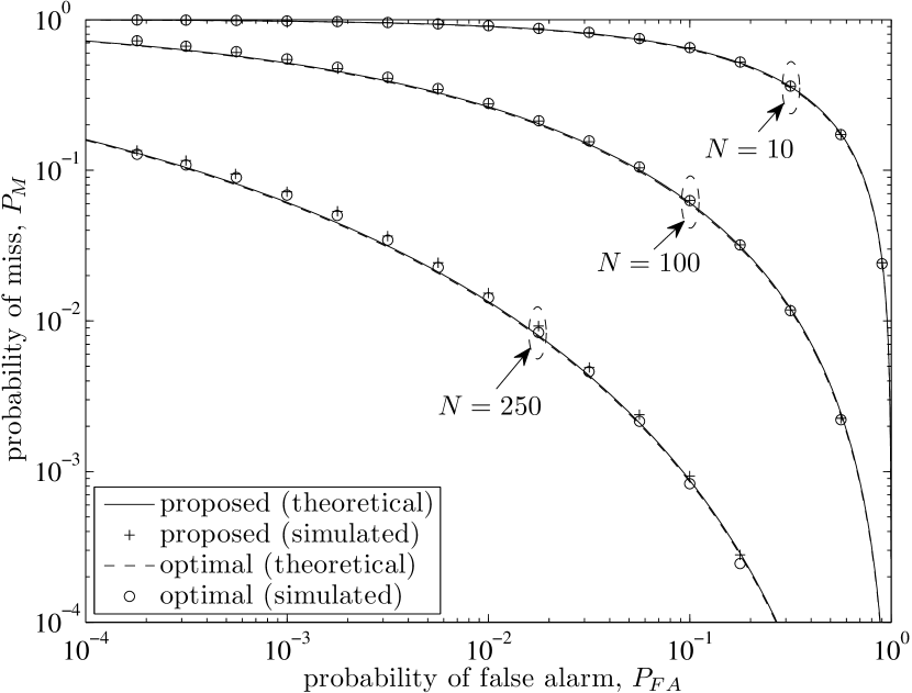
and where the gamma function is defined by [31]. Note that the mean and the variance of the random variable whose CDF is are given by and , respectively. Thus, and of the optimal and the proposed detectors can be computed by using the conditional means and variances of the statistics under and . Fig. 13 shows the ROC curves of the optimal and the proposed detectors for symbol energy per noise density [dB] and , , and , where the theoretical results are evaluated by using (80) while the simulated results are obtained from Monte-Carlo runs. It can be seen that the performance of the detectors is accurately approximated by using the gamma distributions. It can be also seen that the proposed detector performs almost the same as the optimal detector does even when .
VI Conclusions
In this paper, the asymptotic FRESH properizer is proposed as a pre-processor for the block processing of a finite number of consecutive samples of a DT improper-complex SOCS random process. It turns out that the output of this pre-processor can be well approximated by a proper-complex random vector that has a highly structured frequency-domain covariance matrix for sufficiently large block size. The asymptotic propriety of the output allows the direct application with negligible performance degradation of the conventional signal processing techniques and algorithms dedicated to the block processing of proper-complex random vectors. Moreover, the highly-structured frequency-domain covariance matrix of the output facilitates the development of low-complexity post-processors. By solving the signal estimation and signal presence detection problems, it is demonstrated that the asymptotic FRESH properizer leads to the simultaneous achievement of computational efficiency and asymptotic optimality. Further research is warranted to apply this pre-processor to various communications and signal processing problems involving the block processing of a DT improper-complex SOCS random process and to derive such almost optimal low-complexity post-processors.
References
- [1] F. D. Neeser and J. L. Massey, “Proper complex random processes with applications to information theory,” IEEE Trans. Inf. Theory, vol. 39, no. 4, pp. 1293-1302, July 1993.
- [2] P. J. Schreier and L. L. Scharf, “Second-order analysis of improper complex random vectors and processes,” IEEE Trans. Signal Process., vol. 51, no. 3, pp. 714-725, Mar. 2003.
- [3] P. Wahlberg and P. J. Schreier, “Spectral relations for multidimentional complex improper stationary and (almost) cyclostationary processes,” IEEE Trans. Inf. Theory, vol. 54, no. 4, pp. 1670-1682, Apr. 2008.
- [4] G. Tauböck, “Complex-valued random vectors and channels: Entropy, divergence, and capacity,” IEEE Trans. Inf. Theory, vol. 58, no. 5, pp. 2729-2744, May 2012.
- [5] P. J. Schreier and L. L. Scharf, Statistical Signal Processing of Complex-Valued Data: The Theory of Improper and Noncircular Signals. NY: Cambridge Univ. Press, 2010.
- [6] B. Picinbono and P. Chevalier, “Widely linear estimation with complex data,” IEEE Trans. Signal Process., vol. 43, no. 8, pp. 2030-2033, Aug. 1995.
- [7] W. M. Brown and R. B. Crane, “Conjugate linear filtering,” IEEE Trans. Inf. Theory, vol. 15, no. 4, pp. 462-465, July 1969.
- [8] E. Serpedin, F. Panduru, I. Sari, and G. B. Giannakis, “Bibliography on cyclostationarity,” Signal Process., vol. 85, no. 12, pp. 2233-2303, Dec. 2005.
- [9] W. A. Gardner, A. Napolitano, and L. Paura, “Cyclostationarity: Half a century of research,” Signal Process., vol. 86, no. 4, pp. 639-697, Apr. 2006.
- [10] W. A. Gardner and L. E. Franks, “Characterization of cyclostationary random signal processes,” IEEE Trans. Inf. Theory, vol. 21, no. 1, pp. 4-14, Jan. 1975.
- [11] W. A. Gardner, “Signal interception: A unifying theoretical framework for feature detection,” IEEE Trans. Commun., vol. 36, no. 8, pp. 897-906, Aug. 1988.
- [12] W. A. Gardner and C. M. Spooner, “Signal interception: Performance advantages of cyclic-feature detectors,” IEEE Trans. Commun., vol. 40, no. 1, pp. 149-159, Jan. 1992.
- [13] W. A. Gardner, W. A. Brown, and C.-K. Chen, “Spectral correlation of modulated signals: Part II–Digital modulation,” IEEE Trans. Commun., vol. 35, no. 6, pp. 595-601, June 1987.
- [14] W. A. Gardner and W. A. Brown, “Frequency-shift filtering theory for adaptive co-channel interference removal,” in Proc. 23rd Asilomar Conf. Signals, Systems, Computers, vol. 2, Pacific Grove, CA, 30 Oct.- 1 Nov. 1989, pp. 562-567.
- [15] G. B. Giannakis, “Filterbanks for blind channel identification and equalization,” IEEE Signal Process. Lett., vol. 4, no. 6, pp. 184-187, June 1997.
- [16] A. Sabharwal, U. Mitra, and R. Moses, “MMSE receivers for multirate DS-CDMA systems,” IEEE Trans. Commun., vol. 49, no. 12, pp. 2184-2197, Dec. 2001.
- [17] J. H. Cho, “Joint transmitter and receiver optimization in additive cyclostationary noise,” IEEE Trans. Inf. Theory, vol. 50, no. 12, pp. 3396-3405, Dec. 2004.
- [18] Y. H. Yun and J. H. Cho, “An optimal orthogonal overlay for a cyclostationary legacy signal,” IEEE Trans. Commun., vol. 58, no. 5, pp. 1557-1567, May 2010.
- [19] B. W. Han and J. H. Cho, “Capacity of second-order cyclostationary complex Gaussian noise channels,” IEEE Trans. Commun., vol. 60, no. 1, pp. 89-100, Jan. 2012.
- [20] W. A. Gardner, “Cyclic Wiener filtering: Theory and method,” IEEE Trans. Commun., vol. 41, no. 1, pp. 151-163, Jan. 1993.
- [21] B. W. Han and J. H. Cho, “Optimal signaling in second-order cyclostationary Gaussian jamming environment,” in Proc. of IEEE Military Communications Conf. (MILCOM), Baltimore, MD, 7-10 Nov. 2011, pp. 102-107.
- [22] J. Eriksson and V. Koivunen, “Complex random vectors and ICA models: Identifiability, uniqueness, and separability,” IEEE Trans. Inf. Theory, vol. 52, no. 3, pp. 1017-1029, Mar. 2006.
- [23] R. M. Gray, “Toeplitz and circulant matrices: A review,” Found. Trends Commun. Inf. Theory, vol. 2, no. 3, pp. 155-239, 2006.
- [24] Y. G. Yoo and J. H. Cho, “Asymptotically optimal low-complexity SC-FDE in data-like co-channel interference,” IEEE Trans. Commun., vol. 58, no. 6, pp. 1718-1728, June 2010.
- [25] J. H. Yeo and J. H. Cho, “Properization of second-Order cyclostationary random processes and its application to signal presence detection,” in Proc. IEEE Military Communications Conf. (MILCOM), Orlando, FL, 29 Oct.-1 Nov. 2012, pp. 1-6.
- [26] B. Picinbono and P. Bondon, “Second-order statistics of complex signals,” IEEE Trans. Signal Process., vol. 45, no. 2, pp. 411-420, Feb. 1997.
- [27] G. Bi and Y. Chen, “Fast generalized DFT and DHT algorithms,” Signal Process., vol. 65, no. 3, pp. 383-390, Mar. 1998.
- [28] H. V. Poor, An Introduction to Signal Detection and Estimation, 2nd ed. NY: Springer-Verlag, 1994.
- [29] A. van den Bos, “The multivariate complex normal distribution–A generalization,” IEEE Trans. Inf. Theory, vol. 41, no. 2, pp. 537-539, Mar. 1995.
- [30] W. Zhang, H. V. Poor, and Z. Quan, “Frequency-domain correlation: An asymptotically optimum approximation of quadratic likelihood ratio detectors,” IEEE Trans. Signal Process., vol. 58, no. 3, pp. 969-979, Mar. 2010.
- [31] A. Papoulis, Probability, Random Variables, and Stochastic Processes, 4th ed. New York: McGraw-Hill, 2002.
- [32] U. Grenander, H. O. Pollak, and D. Slepian, “The distribution of quadratic forms in normal variates: A small sample theory with applications to spectral analysis,” J. Soc. Ind. Appl. Math., vol. 7, no. 4, pp. 374-401, Dec. 1959.