Discovery of Lyman Break Galaxies at $z\sim 7$ from the ZFOURGE Survey

Abstract

Star-forming galaxies at redshifts $z>6$ are likely responsible for the reionization of the universe, and it is important to study the nature of these galaxies. We present three candidates for $z\sim 7$ Lyman$-$break galaxies (LBGs) from a 155 arcmin² area in the CANDELS/COSMOS field imaged by the deep FourStar Galaxy Evolution (zFourGE ) survey. The FourStar medium-band filters provide the equivalent of $R\sim 10$ spectroscopy, which cleanly distinguishes between $z\sim 7$ LBGs and brown dwarf stars. The distinction between stars and galaxies based on an object’s angular size can become unreliable even when using HST imaging; there exists at least one very compact $z\sim 7$ candidate (FWHM$\sim$0.5-1 kpc) that is indistinguishable from a point source. The medium-band filters provide narrower redshift distributions compared with broad-band-derived redshifts. The UV luminosity function derived using the three $z\sim 7$ candidates is consistent with previous studies, suggesting an evolution at the bright end ($M_{UV}\sim-21.6$ mag) from $z\sim 7$ to $z\sim 5$. Fitting the galaxies’ spectral energy distributions, we predict Lyman-$\alpha\;$ equivalent widths for the two brightest LBGs, and find that the presence of a Lyman-$\alpha\;$  line affects the medium-band flux thereby changing the constraints on stellar masses and UV spectral slopes. This illustrates the limitations of deriving LBG properties using only broad-band photometry. The derived specific star-formation rates for the bright LBGs are $\sim$ 13  Gyr^-1, slightly higher than the lower-luminosity LBGs, implying that the star-formation rate increases with stellar mass for these galaxies.

1. Introduction

Discovering high-redshift ($z>6$) galaxies, and understanding their physical nature is of great importance in studying the early universe because these objects are likely sources for reionization of the intergalactic medium (IGM: Trenti et al., 2010; Salvaterra et al., 2011; Finkelstein et al., 2012, e.g.) at $z\gtrsim$ 7 (Fan et al., 2002; Komatsu et al., 2011). With the advent of large near-infrared (NIR) detectors, significant progress has been made in discovering galaxies at $z\gtrsim 7$ (e.g. Iye et al., 2006; Vanzella et al., 2011; Ono et al., 2012; Schenker et al., 2012), as the rest-frame UV light from these galaxies shifts to $\lambda>$1 $\mu$m.

There are two main techniques for finding high-redshift ($z\gtrsim 7$) galaxies : (1) the Lyman-break or dropout method (e.g. Steidel et al., 1995, 1999; Adelberger et al., 2004; Dickinson et al., 2004; Giavalisco et al., 2004; Ouchi et al., 2004; Bouwens et al., 2007; McLure et al., 2010), selected based on strong absorption in their spectral energy distribution (SED) at wavelengths shortward of redshifted Lyman-$\alpha\;$due to IGM HI absorption, and (2) the narrow-band imaging technique, which identifies galaxies with a strong, redshifted Lyman-$\alpha\;$emission line using narrow-band filters (e.g. Malhotra & Rhoads, 2002; Rhoads et al., 2005; Iye et al., 2006; Kashikawa et al., 2006; Ouchi et al., 2009b; Hibon et al., 2010; Tilvi et al., 2010; Krug et al., 2012). A unique advantage of narrow-band selected galaxies is that these galaxies are more likely to be confirmed via spectroscopic followup because they are pre-selected based on the strong Lyman-$\alpha\;$emission line. On the other hand, LBGs selected via the broad-band dropout method are unbiased in their selection (unlike Lyman-$\alpha\;$selected galaxies), and LBG surveys probe larger cosmological volumes due to broader filters. Currently there are many candidate LBGs (e.g. Bouwens et al., 2007; Ouchi et al., 2009; McLure et al., 2010) at redshifts much greater than $z\sim 7$  (e.g. Bouwens et al., 2011; Bradley et al., 2012; Yan et al., 2011; Finkelstein et al., 2012; Oesch et al., 2012).

With growing samples of $z\sim 7$ galaxies, we are able to calculate the rest-frame UV luminosity function (LF), which is a simple yet powerful probe of the early universe. The luminosity function allows us to constrain the observed number density of star-forming galaxies from which we can estimate (with some assumptions) the number of hydrogen-ionizing photons available to reionize the IGM. In addition, the observed luminosity function allows us to study the galaxy evolution by comparing the number density of galaxies at different redshifts.

Several studies have focused on understanding the evolution of the UV luminosity function from $z\sim 3$ to 6 and find that there is a significant decrease in the number density of UV bright galaxies from low to high redshifts (e.g. Stanway et al., 2003; Shimasaku et al., 2005; Bouwens et al., 2006). If this trend continues, we expect even a greater decline in the number density of galaxies at redshift $z>6$. Current observations at $z>6$ suggest a strong evolution in the characteristic magnitude $\rm M^{\star}\sim$ -19.8 mag (Bouwens et al., 2008; McLure et al., 2010; Ouchi et al., 2009; Yan et al., 2010; Castellano et al., 2010; Bouwens et al., 2010) compared with $\rm M^{\star}\sim$-20.9 mag at $z\sim 4$ (Bouwens et al., 2007). Most of these studies, especially at $z\sim 7$, rely on HST  observations which have the advantage of probing fainter galaxies, however with smaller survey areas. Recently, Ouchi et al. (2009), Castellano et al. (2010), Capak et al. (2011), and Bowler et al. (2012) found several candidates using ground-based observations, which have the advantage of surveying larger areas and thus probing brighter, rarer galaxies.

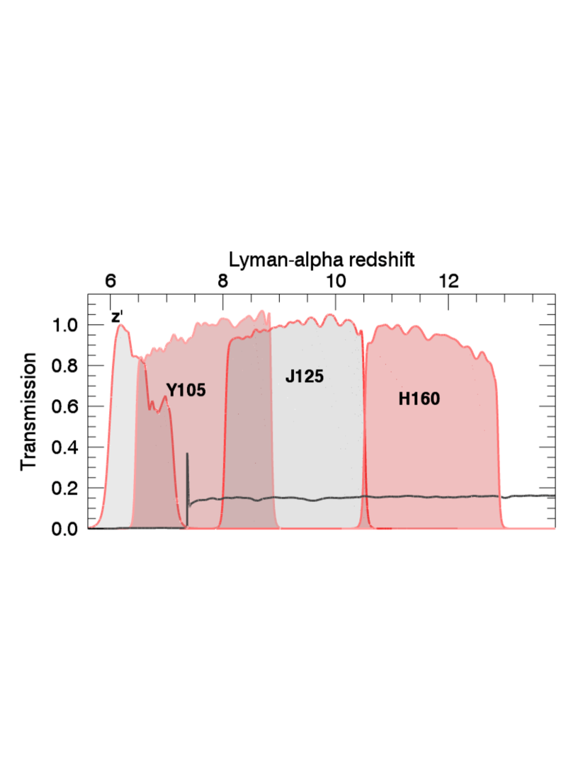
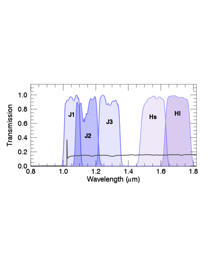
Figure 1.— Filter transmission curves of the FourStar medium-band compared to other broad-band filters. The top panel shows broad-band Subaru $z^{\prime}$, HST Y₁₀₅, J₁₂₅  & H₁₆₀  filters, while the bottom panel shows FourStar medium-band filters J₁, J₂, J₃, H_s  and H_l, which provide R$\sim$10 resolution spectroscopy. Black line shows a template spectral energy distribution of a $z=7.4$ galaxy with the Lyman-$\alpha\;$  emission line falling in the J₁  filter. The top axis marks the Lyman-$\alpha\;$ redshifts as a function of wavelength.

While it is relatively easy to construct the luminosity function, its accuracy depends on a number of systematics, including the degree of contamination of the $z\sim 7$  galaxy sample. It is affected by contaminants that mimic the colors of high-redshift galaxies. The main contaminants of $z\sim 7$ LBGs are Galactic brown dwarfs, low-redshift ($z\sim 1-2$) dust obscured galaxies with very faint continuum in the visible bands, and transient objects. The brown dwarf stars may be separated from (resolved) galaxies using high angular-resolution imaging. However, the ability to resolve galaxies can become unreliable at the faint magnitudes and compact sizes typical of $z\sim 7$ galaxies, even with the HST observations. For example, the rejection of point sources from $z\sim 7$ samples precludes the possibility that some $z\sim 7$ galaxies have morphologies that are unresolved even at HST resolution (FWHM $\approx$0$\farcs$2 which corresponds to 1 kpc at $z=7$), leading to sample incompleteness. These uncertainties need to be accounted for when constructing the luminosity function.

In addition to studying the UV luminosity function, understanding the physical properties of high-redshift galaxies is important to link their evolution during the early stages of galaxy formation to galaxies at other epochs. As we probe redshifts $z\gtrsim 2$, galaxies on average have smaller stellar masses $\sim 10^{10}$ M_⊙ (e.g. Sawicki & Yee, 1998; Papovich et al., 2001; Shapley et al., 2001, 2005; Yan et al., 2005; Erb et al., 2006; Fontana et al., 2006; Reddy et al., 2006; Overzier et al., 2009), bluer UV colors (e.g. Dickinson et al., 2003; Papovich et al., 2004; Labbé et al., 2007; Overzier et al., 2009; Bouwens et al., 2009a), and younger stellar populations with smaller amounts of dust (e.g. Meurer et al., 1999; Papovich et al., 2001; Shapley et al., 2001, 2005; Reddy et al., 2005, 2006, 2008; Reddy & Steidel, 2009; Bouwens et al., 2009a; Finkelstein et al., 2010, 2011). Moreover, the specific star-formation rates (sSFR: the SFR per unit stellar mass) of galaxies at $z\gtrsim 2$ are roughly constant as a function of redshift, with sSFR ranging from $\sim~{}$2 to 6 Gyr^-1, albeit with large uncertainties (e.g. Stark et al., 2009; González et al., 2010; Bouwens et al., 2011; Reddy et al., 2012). In all cases, the physical properties of the most distant galaxies ($z>6$), are derived by fitting the spectral energy distribution templates to the galaxy photometry measured in broad-band filters (e.g. Finkelstein et al., 2011). While some effects such as the degeneracy among different derived parameters are already known, the template fitting to the broad-band photometry may introduce (as of yet) unknown systematic errors on the constraints of these parameters.

Table 1Photometry for COSMOS field.

Filter	$\lambda(\mu m)$	Depth (mag)	Filter width
			$(\rm\AA)$
$g^{\prime}$	0.44	27.96	1384
$r^{\prime}$	0.62	27.95	1460
$i$	0.83	26.59	2270
$z^{\prime}$	0.90	26.43	1384
J1	1.05	26.10	1030
J2	1.14	26.07	1410
J3	1.28	25.69	1320
J125(F125W)	1.25	26.93	2991
Hs	1.55	25.15	1600
Hl	1.70	25.17	1610
H160(F160W)	1.54	27.04	2880
Ks	2.15	25.13	3380
$[3.6]$	3.56	26.0	7274
$[4.5]$	4.52	26.0	9914

• $5\sigma$ depth in 1$\farcs$1 diameter aperture

• $3\sigma$ depth in 2$\farcs$4 diameter aperture (Ashby et al. 2013 submitted)

• Filter width where filter transmission is $>$50%.

• Transmission is $>$30%.
  

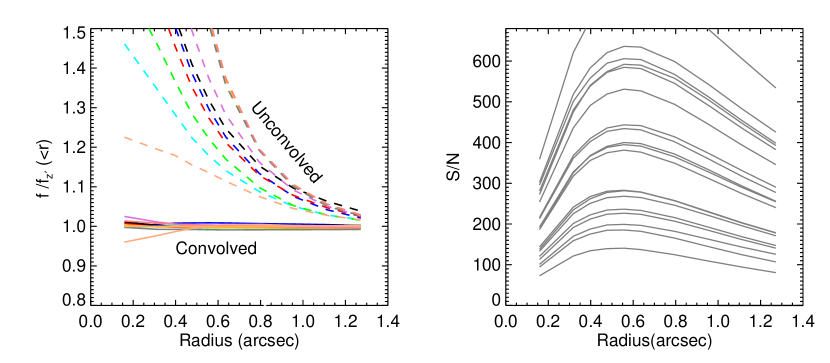
Figure 2.— Left panel: Curves-of-growth for point sources in the convolved and unconvolved images. Dashed and solid lines show flux ratio before and after convolution, respectively, where $f$ is the flux in a given band and $f_{z^{\prime}}$ is the $z^{\prime}$ (reference image) flux enclosed within radius r. Different colors indicate different filters. The flux in aperture radii larger than $0\farcs 48$ among convolved images contribute to $<2$% uncertainty for point sources. Right panel: The signal-to-noise (S/N) for point sources as a function of radii, in the convolved images. Different lines show the S/N of same stars (here shown only the J₃  filter for illustration purposes) that were used for creating the convolution kernel (Section 2). For photometry, we use a circular aperture with $0\farcs 55$ radius as this yields maximum S/N.

The specific goals of this paper are (1) to use near-IR medium-band filters, for the first time, to reliably identify $z\sim 7$ galaxies and to compare the effectiveness of the medium-band technique to that of broad-band photometry; (2) to discuss the contamination rate of brown dwarfs in $z\sim 7$ galaxy samples; and (3) to derive the physical properties of the galaxies from the medium-band photometry and to test for systematic uncertainties on physical properties using broad-band data alone. Photometric redshifts derived using medium-band filters have much narrower probability distributions compared to the broad-band derived photometric redshifts owing to the higher spectral resolution (R$\sim$10) of the medium-band filters. This led to a recent discovery of a distant ($z=2.1$) galaxy cluster in the COSMOS field (Spitler et al., 2012). Owing to very deep imaging and excellent seeing, we are also able to place better constraints on the redshifts and on the evolution of bright star-forming galaxies out to $z\sim 7$.

This paper is organized as follows. Section 2 describes the observations, data reduction, and catalog generation. In Section 3 we present our LBG color selection method and sources of contamination and their identification. Section 4 describes the construction of the UV luminosity function and its comparison to previous studies. We compare the advantage of using medium-band over only broad-band photometry, and its influence on the derived physical properties of high-redshift galaxies in Section 5. We summarize our conclusions in Section 6. Throughout this paper we use AB magnitudes and standard cosmology with $h=0.7$, $\Omega_{\lambda}=0.7$, and $\Omega_{m}=0.3$.

2. Observations and Data Reduction

We observed a 155 arcmin² area in the CANDELS/COSMOS field (Scoville et al., 2007) centered at RA: 10:00:31 and Dec:+02:17:21, using the FourStar instrument, as part of the ongoing FourStar Galaxy Evolution survey (zFourGE ) during 2011-2012. The FourStar instrument (Persson et al.  2013) is a near-IR camera mounted on the Magellan/Baade telescope. It has 4096 $\times$ 4096 pixels with a 0$\farcs$159/pixel resolution and covers a 10′.8$\times$10′.8 field of view. We observed with five adjacent medium-band filters (J₁, J₂, J₃, H_s, H_l: Table 1) with a resolution of $R\sim 10$, and one broad-band (K_s) filter (Labbé et al in preparation). Figure 1 shows filter transmission curves for the FourStar medium-band filters compared to the broad-band filters from Subaru/Suprime ($z^{\prime}$), and HST (Y₁₀₅, J₁₂₅, H₁₆₀) filters. The J₁ filter has a similar central wavelength to the Y₁₀₅ filter (and also to many $Y$-filters on ground-based telescopes), but the J₁ filter is much narrower compared with the HST  Y₁₀₅ filter.

We processed all raw images using a custom designed IDL-based pipeline (described in more detail in Labbé et al in preparation) adapted from the NEWFIRM Medium Band Survey data reduction pipeline (NMBS: Whitaker et al., 2011). The data quality of the FourStar images is excellent and the point-spread function (PSF) FWHM for the stacked FourStar images correspond to 0.55, 0.52, 0.51, 0.51, 0.57, & 0.48 arcsec in the J₁ through K_s filters, respectively. In addition to this data set, we used publicly available data in the optical (Subaru $g^{\prime}$, $r^{\prime}$, $z^{\prime}$, & ACS $i_{814}(i)$), deep near-IR   HST WFC3 J₁₂₅  & H₁₆₀ from the CANDELS survey (Koekemoer et al., 2011; Grogin et al., 2011), and infrared IRAC (Fazio et al., 2004) data. We also used deep 3.6 and 4.5$\mu$m images (Ashby et al 2013 submitted) from the Spitzer Extended Deep Survey ($SEDS$); 5.8 and 8.0$\mu$m data from the Spitzer Space Telescope (Werner et al., 2004). Table 1 presents the central wavelengths and limiting magnitudes for the zFourGE data as well as information for the ancillary data.

The PSF among different bands varies due to differing central wavelengths, different instruments used for imaging, and in the case of ground-based observations, due to different seeing conditions. We convolved all images to a reference image having the broadest PSF-FWHM (in our case the Subaru $z^{\prime}$ image with PSF FWHM=0$\farcs$8). In each band, we first constructed an empirical PSF by identifying stars and stacking them with their centers aligned. We then used an IDL routine, DECONV$\_$TOOL (Varosi & Landsman, 1993), to construct a kernel to convolve the image PSF to match the stellar PSF. Figure 2 shows the curve-of-growth of point sources in the images following the convolution process. As shown in the figure (left panel), the relative flux for point sources in each band is matched to better than 2% for all apertures with radii larger than $0\farcs 47$.

The photometry in circular apertures was optimized for faint, compact sources. Figure 2 (right panel) shows the S/N for point sources measured in circular apertures as a function of aperture radius. The S/N is maximized for point sources with apertures of radii $0\farcs 55$. Therefore we use circular apertures with diameter of $1\farcs 1$ for the photometry in our analysis.

2.1. Spitzer/IRAC Photometry

As mentioned earlier, to extend the wavelength coverage of our candidates and to derive the physical properties as accurately as possible, we used recent deep Spitzer IRAC data (Ashby et al 2013 submitted) in two bands (3.6 $\mu m$, 4.5 $\mu m$) obtained from the SEDS survey. However, due to its low resolution, neighboring objects tend to blend resulting in incorrect flux measurements. To circumvent this issue, we used GALFIT (Peng et al., 2002) code to measure the object fluxes, as described below. First, we fit the two dimensional surface brightness profiles of all objects within 7″ of the $z\sim 7$ candidate (excluding the $z\sim 7$ galaxy) and subtracted these fits to obtain a residual image. We then measured photometry of the $z\sim 7$ candidates from the IRAC data using the IDL procedure APER, measuring the flux in a fixed 2″ diameter aperture and correcting to the total flux using the aperture corrections derived by taking the ratio between 2″ and 15″  diameter aperture fluxes of isolated sources. Finally, we derived the uncertainties by measuring the $rms$ in apertures of the same size as above, randomly placed in regions devoid of objects in the IRAC images.

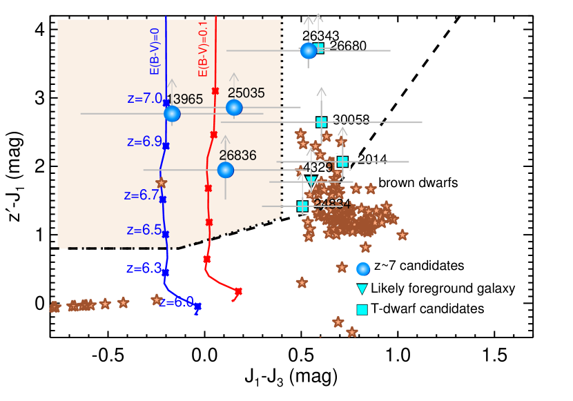
Figure 3.— Color-color plot for $z\sim 7$  LBG candidate selection. Filled circles, triangle and square symbols indicate all the objects that pass the LBG selection criteria (Equation 1; dashed line), adapted from Oesch et al. (2010). Blue and red lines show the expected colors of a star-forming stellar population, for two extinction values, as a function of redshift (redshifts indicated for reference) using models from Bruzual & Charlot (2003). Star symbols show the expected colors of very late-type stars derived from observed spectra of M, L, and T-dwarf stars. The initial color selection (dashed line) yields four $z\sim 7$  LBG candidates (filled circles), four brown dwarf stars (filled squares) and one likely foreground galaxy (filled triangle). Based on the galaxy tracks (blue and red lines ) and brown dwarf star colors, we refined the $z\sim 7$ LBG selection criteria (Equation 4; shaded region) that eliminates most of the nearby stars. This new selection yields three robust $z\sim 7$  LBG candidates.

2.2. Source Catalogs

We identified sources in each of the images using Source Extractor software (SExtractor : Bertin & Arnouts, 1996) in dual image mode. In this mode, a detection image is used to identify the pixels associated with each object, while the fluxes are measured from a distinct photometry image. For the detection image, we used a $\chi^{2}$ image, which optimally sums multiple images (accounting for varying S/N) for source detection (Szalay et al., 1999). The $\chi^{2}$ image ($J_{chq}$) was constructed from the J₁, J₂, J₃  images using SWarp (Bertin et al., 2002). We measured object photometry from the PSF-matched images in a fixed aperture size of 1.1″ diameter.

While SExtractor estimates the noise for each object, this estimate is incorrect in the convolved images as it does not account for correlated noise, which results from the image reduction and convolution processes. To estimate the flux uncertainty for each object in the convolved images we followed an empirical approach described in Labbé et al. (2003). To estimate the pixel-to-pixel noise we measured the rms background variation as a function of linear size $\rm N=\sqrt{A}$ where $A$ is the area of an aperture. First, we measured the sky flux in increasingly larger apertures that are randomly placed in the PSF-matched-convovled image, taking care to avoid detected objects. From the distribution of fluxes measured in a given aperture size, we measured the standard deviation, $\sigma$. The 1$\sigma$ error on the flux was then calculated using equation 5 from Whitaker et al. (2011). Our final catalog contains aperture fluxes obtained from PSF-matched images in $g^{\prime}$, $r^{\prime}$, $i$, $z^{\prime}$, J₁, J₂, J₃, J₁₂₅, H_s, H_l, H₁₆₀, and K_s along with flux uncertainties.

2.3. Photometric Redshifts

We derive photometric redshifts using the photometric redshift code EAZY (Brammer et al., 2008) taking advantage of extensive multi-wavelength data publicly available in the COSMOS field for finding the best-fit solution to the observed data. The EAZY code (v2.1; Brammer et al., 2011) contains seven different templates spanning a large range of galaxy colors and incorporates nebular emission lines. While our $z\sim 7$ candidate selection is based primarily on a color-color selection, to increase the reliability of our candidates, we also require that each of the candidates have photometric redshifts $z>6$.

3. LBG Color Selection at $z\sim 7$

Our initial color-selection criteria to identify candidate galaxies at $z\sim 7$ is adapted from Oesch et al. (2010);

$$\mathrm{S/N}(J_{chq}) >7.0$$ (1)

$$\mathrm{S/N(optical)} <2.0,$$

$$\textit{J${}_{1}$}-\textit{J${}_{3}$} <1.3\;\rm{mag},$$

$$z^{\prime}-\textit{J${}_{1}$} >0.8\;\rm{mag},$$

$$z^{\prime}-\textit{J${}_{1}$} >0.9+0.75(\textit{J${}_{1}$}-\textit{J${}_{3}$})\;\rm{mag},$$

$$z^{\prime}-\textit{J${}_{1}$} >-1.1+4(\textit{J${}_{1}$}-\textit{J${}_{3}$})\;\rm{mag}.$$

Similar criteria have been used in other studies to identify $z\sim 7$ galaxies (e.g. Bouwens et al., 2009a; Ouchi et al., 2009; Castellano et al., 2010). In addition to these criteria, we required that each of the candidates be detected in the J₂ filter as this filter is very effective in discriminating T-dwarf stars (Tilvi et al in preparation), due to their methane and water absorption features (Tinney et al., 2012), from high-redshift star-forming galaxies.

Figure 3 shows a J₁-J₃  vs $z^{\prime}$-J₁  color-color plot and illustrates the region (dashed line) that corresponds to the selection criteria of Equation 1. Color-color tracks of star-forming galaxies with two different dust attenuation are shown in blue and red lines with redshift labels. These tracks are obtained from Bruzual & Charlot (2003) stellar population synthesis models by integrating the model spectral energy distributions with the $z^{\prime}$, J₁, and J₃  filter. The models assumed E(B-V)= 0.0 (blue line) and 0.1 (red line) with Z=0.2Z_⊙ metallicity, constant star-formation history, IGM opacity taken from (Meiksin, 2006), and a constant age of $t$= 100 Myr. Based on these color tracks it can be seen that the star-forming galaxies occupy a specific region of the color-color space.

We identified 9 objects in total satisfying the selection criteria from Equation 1. Based on several tests described in the following sections, out of the 9 objects in the initial sample (hereafter initial source list), four objects are identified as $z\sim 7$ LBG candidates, four objects are identified as brown dwarf stars and the remaining object is identified as a likely foreground dust-obscured galaxy at $z<3$. To minimize the contamination from stars and foreground galaxies, we further refine the color-color selection (Section 3.3) that include only the robust $z\sim 7$ LBG candidates (Figure 3; shaded region). Figure 4 shows postage stamps of these $z\sim 7$ LBG candidates, as well as one likely T-dwarf star for comparison.

3.1. Sources of Contamination

The color-color selection of $z\sim 7$  LBG candidates suffers from several possible sources of contamination including image artifacts (or spurious detections), nearby cool brown dwarf stars which mimic high-redshift galaxy colors, intermediate redshift galaxies with faint continuum in the visible bands, and transient sources including supernovae or asteroids. In this and the following sections we discuss in detail the likelihood of any of these contaminating sources entering the initial source list.

3.1.1 Spurious detections

In the $z\sim 7$  LBG selection, we require that each of the objects is detected with S/N $>4$ in more than one band redward of the $z^{\prime}$  filter. This requirement makes spurious detections due to either background or electronic noise extremely unlikely.

3.1.2 Transient/High-proper motion objects

It is possible that transient objects including asteroids, and supernovae can be detected in more than one band. However, with the availability of two epoch data, separated by about one year, we can eliminate any transients by comparing their positional shift between the two epochs. Therefore, we conclude that the initial source list does not contain any transient sources.

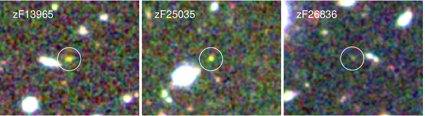
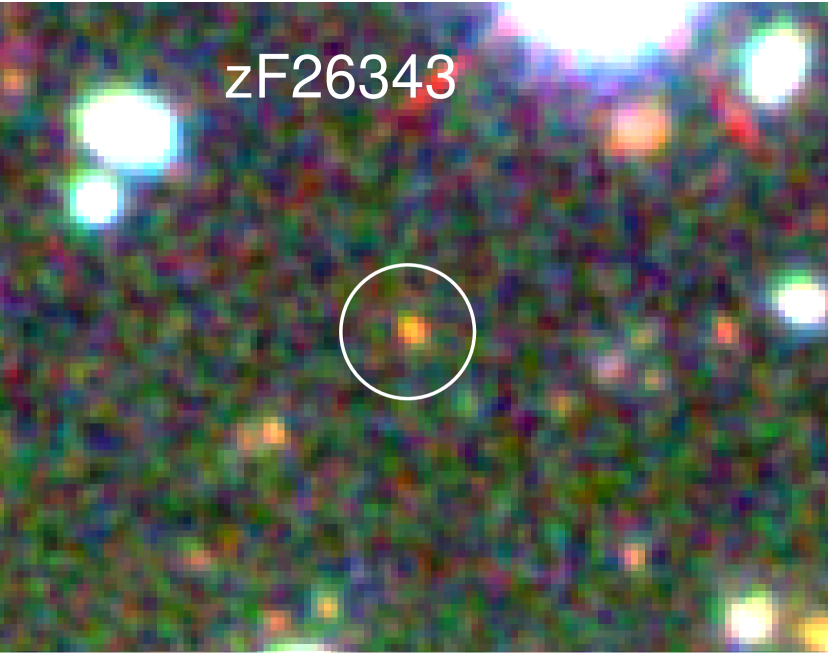
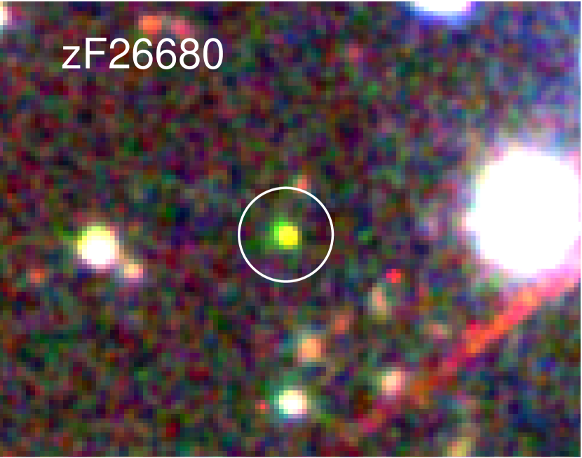
         g’     r’     i      z’    J1     J2    J3    J125    Hs     Hl   H160     Ks    [3.6] [4.5]  [5.7]   [8]

zF26836    zF25035     zF13965

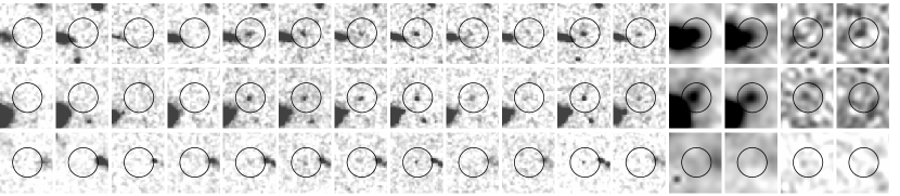
  $\mathcal{P}_{6}$=0.99 $\mathcal{P}_{6}$=0.99   $\mathcal{P}_{6}$=0.99

 zF26343

  $\mathcal{P}_{6}$=0.99

$\rm\;Tdwarf$

 zF26680

$\mathcal{P}_{6}$=0.99

Figure 4.— Image cutouts of four $z\sim 7$  LBGs and one of the T-dwarf candidates (zF26680). Top panel shows color composite ($z^{\prime}$,J₁,H₁₆₀) image cutouts while lower two panels show image cutouts in the individual filters. The four $z\sim 7$ LBG candidates (zF13965, zF25025, zF26836, zF26343) ) are selected from the color-color selection (Equation 1) while zF26343 is excluded in the refined color-color selection (Equation 4). Each candidate is marked within a 2″  radius circle. These candidates are clearly detected in at least one of the medium-band filters while undetected ($<2\sigma$) in any of the visible bands. The integrated probability distribution $\mathcal{P}_{6}$  (Equation 2) is shown on the right side. In addition to satisfying the color-color selection criteria, each of the candidates is required to have $\mathcal{P}_{6}$$>0.7$ and S/N$<2$ in the visible $\chi^{2}$ image. These two criteria minimizes the contamination from low-redshift galaxies. In the bottom panel, we show one of the candidate T-dwarf stars that was selected in the initial color-color selection (Oesch et al 2010). Such T-dwarf stars can be cleanly distinguished from galaxies using medium-band photometry.

3.1.3 Foreground galaxies

While the $z\sim 7$  candidates are required to have no detection ($<2\sigma$) in the observed visible bands, it is possible that the initial source list contains foreground objects, likely $z\sim 1-3$ highly dust obscured galaxies that have very low fluxes in the visible bands, but are bright in the near-IR and IRAC bands, (see Labbé et al 2005, Papovich et al 2006). These low-redshift galaxies cannot be completely ruled out, but the contamination from such objects can be minimized because they occupy a specific color-color space (Figure 3) compared to the $z\sim 7$  galaxies which have bluer colors. Furthermore, many of the red, intermediate redshift galaxies at $z\sim 1-4$ have bright IRAC fluxes with typical colors $[4.5]-[5.8]\lesssim 0$ AB mag (e.g. Yan et al., 2004), which distinguishes them strongly from $z\sim 7$  galaxy candidates. In addition to these signatures, the photometric redshifts can provide an additional constraint on the likelihood of an object being a low-redshift galaxy.

In order to compute the likelihood of our candidates being $z\sim 7$  galaxies, we followed a similar procedure, as described in Finkelstein et al. (2010). We compute the total redshift probability distribution $\mathcal{P}_{6}$ given by

$$\mathcal{P}_{6}=\frac{\int_{6}^{9}{\tiny P(z)\,dz}}{\int_{0}^{9}P(z)\,dz},$$ (2)

where $\int_{6}^{9}P(z)dz$ is the integrated probability distribution from $z=6$ to $z=9$. This probability distribution is normalized by $\int_{0}^{9}P(z)dz$ such that $\mathcal{P}_{6}\leq 1$. We make use of the probability distribution $P(z)$ derived using the photometric redshift code EAZY and require that each of the $z\sim 7$  candidates has $\mathcal{P}_{6}>0.7$. This means that each of the $z\sim 7$  candidates has greater than $70\%$ probability of being a $z>6$ galaxy, based on the photometric redshift. All of the 9 objects in the initial source list have $\mathcal{P}_{6}>0.99$ and in principle, we could restrict the sample to the stricter requirement of $\mathrm{P}_{6}>0.99$, but this would have risked missing some $z\sim 7$  galaxies near our detection limit (see Finkelstein et al., 2010).

3.1.4 Visible $\rm\chi^{2}$ Image

To further test the reliability of $z\sim 7$  candidates’ non-detection in the individual visible bands, we combine $g^{\prime}$, $r^{\prime}$, and $i$ images to construct a visible $\rm\chi^{2}$ image; the combined $\rm\chi^{2}$ image is significantly deeper than individual images. We then run SExtractor to measure the S/N of all objects in the $\rm\chi^{2}$ image. Based on S/N($>2$) in the visible $\rm\chi^{2}$ image, we reject one object (zF4329) out of 9 objects from the initial source list, as being a likely foreground galaxy with very faint continuum. This rejection is also supported by its strong detection in the MIPS (Rieke et al., 2004) 24$\mu m$ flux; there are no MIPS detections for any of the remaining objects.

3.2. Distinguishing Stars from Compact Galaxies

Galactic brown dwarfs ($M$, $L$, and $T$ ) are one of the main contaminants because their near-IR colors resemble high-redshift ($z\sim 7$) galaxy colors. While it is possible to identify candidates for stars using their FWHM and stellarity index (produced by SExtractor) when using HST observations, these classifiers tend to become unreliable at fainter magnitudes. In addition, at high-redshifts we expect some galaxies to be very compact with their FWHM ($<1$ kpc at $z\sim 7$) comparable to the PSF FWHM. In such cases, even with HST observations, it would be challenging to discriminate between stars and compact galaxies.

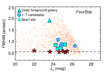
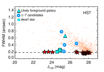
Figure 5.— FWHM as a function of magnitude. Stars (star symbols) are identified based on their FWHM and stellarity index $>$0.8 extracted from SExtractor. Filled symbols (same as in Figure 3) show all objects that passed the initial $z\sim 7$  color selection. Top panel: J₂ mag vs FWHM from the FourStar bands (ground-based observations). Bottom panel: J₁₂₅  mag vs FWHM (space-based observations). The distinction between stars and compact high-redshift galaxies, based on their FWHM, is unreliable from ground-based observations, compared with HST observations. All fours dwarf stars (square symbols) have stellarity indices $>$ 0.7 while object zF25035 has a stellarity index of 0.6 despite being its FWHM similar to the stellar FWHM. Small dots represent all other objects in the catalog. For clarity purposes, we show only a few representative objects. Note that the J₁₂₅ magnitude for the foreground object (triangle) is significantly fainter compared with the J₂ magnitude due to the fact that in the raw (0$\farcs$06) J₁₂₅ image, this object is identified as three different objects.

 

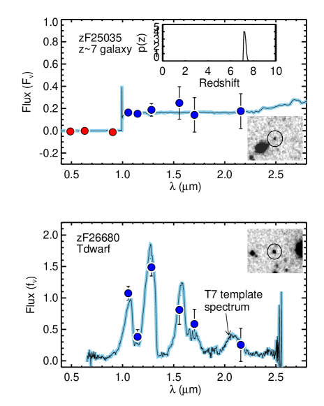
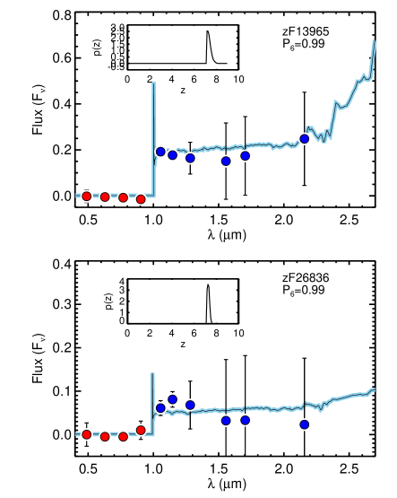
Figure 6.— Spectral energy distributions (SEDs) of the three $z\sim 7$  LBG candidates and one of the T-dwarf candidates. For all panels the filled circles represent observed photometry. For the three panels showing the $z\sim 7$  LBG candidates (zF25035, zF13965, zF26836) the solid line shows the best-fit SED template and the inset panel shows the photometric probability distribution obtained from the EAZY code. In the left panels, also shown are the image cutouts of the LBG candidate (top left) and T-dwarf candidate (lower left panel). For one of the the T-dwarf candidates (lower left panel), the solid line represent the best-fit brown dwarf template spectrum, derived by minimizing $\chi^{2}$ between the FourStar photometry and the expected flux density synthesized from spectral templates of M, L, and T-dwarf stars from Burgasser et al. (2006). The medium-band photometry clearly traces the T-dwarf observed template spectrum (lower left panel) and can distinguish between different T-dwarf types (Tilvi et al., in preparation).

In the following subsections, we perform three tests to distinguish stars from compact galaxies: (i) tests comparing the objects’ FWHM and stellarity indices, (ii) tests of the objects’ spectral features indicative of molecular absorption in stellar atmospheres of brown dwarf stars, and (iii) tests of the objects’ surface brightness profiles.

3.2.1 Identifying Stars using FWHM and Stellarity Index

Figure 5 shows the FWHM (obtained from SExtractor) for objects as a function of J₂  magnitude as well as the FWHM measured in the (unconvolved) HST J₁₂₅ band to compare ground-based data with the space based observations. The horizontal dashed line in each panel of Figure 5 indicates the stellar PSF FWHM obtained by stacking ten isolated stars in the respective images.

In addition to the FWHM, SExtractor produces a stellarity index (CLASS STAR), which determines a likelihood of an object being either a point or an extended source using the self-training of a neural network. A stellarity index closer to 1 is likely a point source while extended objects like galaxies have stellarity indices closer to 0. Figure 5 (top panel), shows some objects classified as stars based on their high ($>0.8$) stellarity index (star symbol). All objects in the initial source list are shown in filled circle, box, or triangle symbols. As can be seen from the top panel, most of the objects appear to be resolved in the FourStar image. However, this appears to be due to the seeing conditions and the magnitude limit of the ground-based data. The lower panel in Figure 5 shows that five of the objects in our sample (zF2014, zF24834, zF30058, zF26680, and zF25035) have FWHM in the HST image much closer to that of a point source. Four of these objects (square symbols in Figure 5) have high stellarity indices ($>$0.7), indicating that they are likely point sources. In fact, fitting brown dwarf spectral templates to the medium-band observations (Section 3.2.2), we conclude that all four of these are candidates for brown dwarf stars. The remaining compact source, zF25035 has a stellarity index of 0.6, suggesting that it might be a compact galaxy rather than a point source. In the following sections, we discuss additional tests to distinguish between the possibility that this object is a point source, or a very compact $z\sim 7$  galaxy candidate.

3.2.2 Spectral Fitting to Medium-band Photometry

Due to the availability of medium-band photometry, in addition to using stellarity indices and FWHM, we can use a spectral fitting technique whereby observed spectral templates are fitted to the medium-band photometry. This method works very well especially in identifying T-dwarf stars because the central wavelengths of the FourStar medium-band filters trace the strong absorption features of T-dwarf stars; this would not be possible using broad-band photometry. van Dokkum et al. (2009) have shown one of the ways to identify T-dwarf stars using medium-band photometry from NEWFIRM (see their Figure 5).

To identify dwarf stars, we synthesized medium-band photometry from the M, L, and T-dwarf observed spectra (Burgasser et al., 2006) and fit these to the FourStar photometry of all candidates to obtain the minimum $\chi^{2}$ between the candidate photometry and the dwarf template spectra. Figure 6 demonstrates the effectiveness of medium-band filters in identifying T-dwarf stars and best-fit spectral energy distribution (SED) of $z\sim 7$ LBGs. The bottom-left panel shows the best-fit spectrum of an observed T-dwarf star, which clearly traces the medium-band photometry, while the remaining panels show $z\sim 7$  candidates fitted with galaxy SEDs. Using this method, we classify four objects, previously identified as stars based on their J₁₂₅ FWHM, as dwarf stars. For the compact object (zF25035) however, we did not find a good fit with any of the M, L, or T-dwarf observed spectra. Thus, this test favors the conclusion that this object is a compact $z\sim 7$  galaxy.

3.2.3 Surface Brightness Profile

Figure 7 shows the surface brightness (J₁₂₅) profiles of five objects: two T-dwarf candidates (with medium-band colors indicative of brown dwarfs and high stellarity); two $z\sim 7$  candidate galaxies including the compact zF25035, and a random object selected from the subsample of all objects with stellarity $>0.9$. The two T-dwarf stars both have stellarity indices $>$0.9 and have FWHM nearly equivalent to the expected WFC3 PSF FWHM (0$\farcs$2). Their surface brightness profiles are also indistinguishable from each other. While the compact $z\sim 7$  galaxy has a FWHM equal to that of the point sources, its surface brightness profile resembles the other $z\sim 7$  candidate galaxy. This is also supported by its lower stellarity index of 0.6 and thus strengthens our earlier conclusion that this object (zF25035) is a compact $z\sim 7$  LBG candidate. Moreover, it shows that at $z\sim 7$, there is a population of very compact (FWHM $\lesssim$1 kpc) star-forming galaxies that are unresolved in typical image quality of ground-based imaging. Note however, that the FWHM or surface brightness profile can become unreliable at fainter magnitudes.

To demonstrate this, we have chosen a random star-like object with stellarity $>0.9$ and FWHM similar to those of the compact galaxy, but with slightly fainter magnitude. As illustrated in Figure 7 (grey dashed line), the surface brightness profile of the random object is indistinguishable from galaxies despite its stellar-like FWHM. This comparison demonstrates that the star versus compact galaxy classification based on either FWHM, stellarity index, or even surface brightness profile would lead to mis-identification, especially at fainter magnitudes ($H\gtrsim 25$ mag), even with HST-like image quality. In such cases, the near-IR medium-band photometry will allow us to cleanly distinguish between the spectral features of brown dwarf stars and $z\sim 7$  galaxy candidates.

In summary, out of five compact objects, four objects are classified as brown dwarf stars, and the remaining object zF25035 is classified as a compact galaxy. Eliminating such objects due to their misidentification could affect the bright end of the UV luminosity function where objects are rare. This may especially be of concern for the case of ground-based data when such compact galaxies are unresolved.

3.3. Final Sample and New Selection Criteria using Medium-bands

Using the initial color selection criteria defined in Equation 1, out of the 9 objects in the initial source list, four objects are identified as nearby dwarf stars based on their FWHM and spectral template fitting test, one object is likely a foreground galaxy based on the S/N($>2$) in the visible $\chi^{2}$ image, and the remaining four objects are identified as $z\sim 7$  LBG candidates. To select the most robust $z\sim 7$  LBG candidates, we revise the $z\sim 7$  candidate selection criteria using medium-band filters as follows.

$$\mathrm{S/N}(J_{chq}) >7.0$$ (3)

$$\mathrm{S/N}(\textit{J${}_{2}$}) >4.0$$

$$\mathrm{S/N(\chi^{2}_{visible})} <2.0,$$

$$\textit{J${}_{1}$}-\textit{J${}_{3}$} <0.4\;\rm{mag},$$

$$z^{\prime}-\textit{J${}_{1}$} >0.8\;\rm{mag}.$$

This color-color selection is indicated in Figure 3 as the shaded region within the dotted polygon. As can be seen, this color-color selection isolates $z\sim 7$  galaxy candidates from both low-redshift red galaxies and brown dwarf stars. Therefore, our new color selection criteria using the FourStar medium-band filters appears to provide a $z\sim 7$  LBG sample that is free of contaminants, although future surveys (including spectroscopic confirmations) are needed to confirm this. The photometry of all three $z\sim 7$  candidate galaxies is shown in Table 1, while Figure 4 and Figure 6 show postage stamps and best-fit SEDs obtained from EAZY, respectively.

While this refined selection yields three robust $z\sim 7$  LBG candidates, one of the candidates (zF26343 in Figure 3) is excluded by this selection (which would have been selected if we had used the selection criteria from Equation 1), and will lead to sample incompleteness thereby affecting the UV luminosity function. We prevent this incompleteness by simulating the effective survey volume that is enclosed within the shaded region in Figure 3.

Table 2Photometry of candidate galaxies at $z\sim 7$.

ID	RA	Dec	$z^{\prime}$	J1	J2	J3	J125	Hs	Hl	H160	Ks	$[3.5]$	$[4.5]$
zF13965	150.12579	2.26662	$>$27.4	25.15	25.24	25.32	25.13	25.41	25.25	25.06	24.87	24.04	24.80
			-	$\pm$0.06	$\pm$0.07	$\pm$0.22	$\pm$ 0.01	$\pm$0.56	$\pm$0.50	$\pm$0.01	$\pm$0.42	$\pm$ 0.20	$\pm$0.20
zF25035	150.09906	2.34362	$>$27.4	25.32	25.39	25.17	25.33	24.86	25.47	25.37	25.24	25.58	23.64
			-	$\pm$0.06	$\pm$0.06	$\pm$0.15	$\pm$0.02	$\pm$0.30	$\pm$0.56	$\pm$0.02	$\pm$0.45	$\pm$ 0.50	$\pm$0.20
zF26836	150.08658	2.31785	$>$27.4	26.39	26.09	26.28	26.68	27.09	27.06	26.47	27.45	$>$26.0	$>$26.0
			-	$\pm$0.14	$\pm$0.11	$\pm$0.41	$\pm$0.05	$\pm$2.26	$\pm$2.31	$\pm$0.11	$\pm$3.41	-	-
zF26343	150.07767	2.35306	$>$27.4	25.79	25.72	25.25	25.35	25.45	24.91	25.02	25.11	24.35	24.42
			-	$\pm$0.11	$\pm$0.10	$\pm$0.21	$\pm$0.02	$\pm$0.65	$\pm$0.43	$\pm$0.05	$\pm$0.51	$\pm$0.20	$\pm$0.20

• All magnitudes are total magnitudes.

• Limiting magnitudes ($2\sigma$ limits in 1$\farcs$1 diameter aperture): $g^{\prime}$=28.9; $r^{\prime}$=28.9; $i$=27.6.

• This candidate falls outside the refined color selection.
  

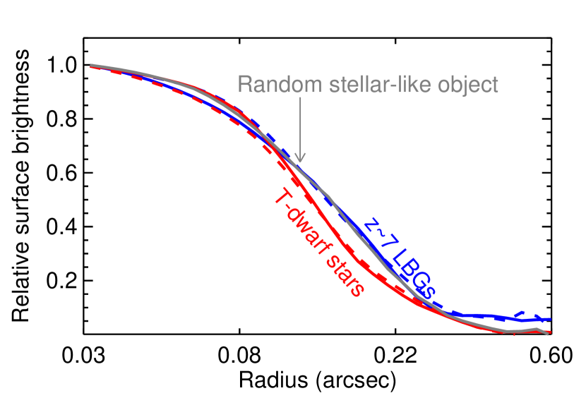
Figure 7.— Comparison of surface-brightness profiles (J₁₂₅) of the compact $z\sim 7$  galaxy candidate (zF25035) and point sources with stellarity index $>$0.9. Blue and red lines show surface brightness profiles of $z\sim 7$  LBG candidates and T-dwarf candidates, respectively. Dot-dashed line is a random object chosen to have similar magnitude and FWHM as those of the compact galaxy, except that this random object has stellarity index $>0.9$ identifying it as a star. If we were to identify this random object based on its FWHM or stellarity index it would be classified as a star, even though its surface brightness profile resembles a non-stellar object. With typical ground-based image quality, and even with HST  image quality, discrimination between galaxies and stars based on their stellarity index is unreliable especially at fainter magnitudes.

4. Luminosity Function at $z\sim 7$

The UV luminosity function provides a direct observational measurement on the number density of star-forming galaxies at a given redshift. We derive the completeness-corrected luminosity function $\phi(m)$ as

$$\phi(m)=\frac{1}{dm}\frac{N(m)}{V_{\rm eff}},$$ (4)

where $N(m)$ is the number of detected objects with magnitude between $m$ and $m+dm$, and $\rm V_{eff}$ is the effective survey volume.

4.1. The Effective Survey Volume

In order to accurately estimate the observed luminosity function we must calculate the effective survey volume since this volume depends on both the apparent magnitude of the selected objects and their redshift distributions. We estimate the effective volume $(V_{\rm eff})$ as described in Steidel et al. (1999):

$$V_{\rm eff}(m)=\int\frac{dV(z)}{dz}p(m,z)\;dz,$$ (5)

where $p(m,z)$ is a probability of detecting a galaxy of apparent magnitude $m$ at redshift $z$ specific to the image quality, depth, and passbands of our dataset, and $dV/dz$ is the comoving volume in a redshift interval $dz$.

In addition, due to photometric errors, objects can scatter in and out of the color-color selection region (shaded region; Figure 3). In the following sections we describe how we estimate the effective volume of our survey. In short, we first compute $p(m,z)$ by inserting and then recovering artificial galaxies in the real images as a function of apparent magnitude and redshift. We then calculate $dV/dz$ for each redshift bin.

4.1.1 Modeling the Colors of High-$z$ Galaxies

To generate artificial galaxies that are representative of high-z galaxies, we created a grid of spectral energy distributions (SEDs) of star-forming galaxies using the Bruzual & Charlot (2003) models. In these models we used the Chabrier initial mass function, solar metallicity, and exponentially rising star-formation history. For a given redshift, we simulated the effect of dust and IGM using the Calzetti (1997) starburst model and the Meiksin (2006) IGM prescription, respectively. We then convolved the resultant SEDs to calculate the bandpass magnitudes and colors through the $z^{\prime}$  and J₁ filters at various redshifts (see Figure 3).

To calculate the J₁-J₃ colors, we followed a different procedure instead of using galaxy tracks because the model colors are nearly constant (see Figure 3) over the redshift range we are currently probing. Here we assumed that the flux at a given wavelength can be described as $f_{\lambda}\propto\lambda^{\beta}$ where $\beta$ is the UV continuum slope. For a given J₁ magnitude (calculated from the model SEDs as described in the previous paragraph), we calculate the J₃  magnitude assuming $\beta=-2.0$. This value of $\beta$ is consistent with $z\sim 7$ galaxies (Finkelstein et al., 2011).

4.1.2 The Probability Function p(m, z)

We computed the probability function (completeness function) by inserting artificial sources based on their redshifts and colors, and recovering these artificial objects using the same procedure as for the real galaxies. Now that we have magnitudes and colors of high-z galaxies as a function of redshift, we first have to create an artificial object with some shape, and assign it a magnitude. To create an artificial galaxy with its shape as close as a real observed galaxy, we choose a random object in a given magnitude bin from the science image itself (in this case J₁).

To insert this object in the $z^{\prime}$, J₁, and J₃ images we choose 500 random positions avoiding any already existing sources ($>3\sigma$ flux) in the J₁ image. Each object was assigned  a $z^{\prime}$, J₁, and J₃  magnitude based on the slope $\beta$, and the color obtained from SED models, respectively. We simulate artificial sources in a redshift bin of 0.2 and magnitude bin $dm=0.1$ mag. We then compute the recovered fraction by taking the ratio of recovered sources (using the selection criteria as described in Section 3.3) to the inserted number of objects. This completeness accounts for both the detection incompleteness as well as the imperfect object selection due to photometric errors leading to additional incompleteness. To increase the number of simulated galaxies without increasing the crowding of sources in a single image, we repeat this procedure ten times for a given redshift and magnitude bin and then average the recovered fraction.

As an illustration we show p(m,z) for J₁=24.8 mag in Figure 8 (shaded area). To compare this completeness function to the broad-band filters, we also overplot the completeness function for the $z\sim 7$  selection using the $F_{850}$, Y₁₀₅, and J₁₂₅  filters from Oesch et al. (2012) and Bouwens et al. (2012). We clearly see a broader completeness function for broad-band filters compared to our medium-band selection. In contrast, at J₁=24.8 mag, $p(m,z)$ is much lower than that derived from much deeper HST  broad-band surveys. Now that we have $p(m,z)$, we calculate the effective volume by integrating the product of $p(m,z)$ and $dV/dz$ (equation 5).

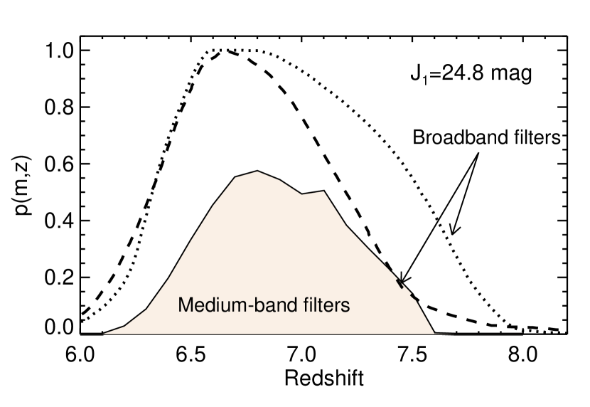
Figure 8.— Probability of recovering artificial galaxies in our survey, shown for a source with J₁=24.8 mag (filled curve). Dashed and dotted lines show HST broad-band completeness function from Oesch et al (2009) and Bouwens et al (2012), respectively. The broad-band completeness distribution achieves a higher peak $p(m,z)$ due to the HST survey depths, but is slightly broader compared to the FourStar completeness distribution. The narrower distribution of medium-bands allows for much tighter redshift probability distribution.

Figure 9.— Binned UV luminosity function at $z\sim 7$. Blue filled circles represent the number densities of our $z\sim 7$  sample in two rest-frame magnitude bins with $dM$=1 mag. Error bars on the abscissa show the width of the magnitude bin. Error bars in the ordinate are a posteriori errors, calculated by marginalizing over all Poisson distributions given the observed number of two objects in the brighter bin and one object in the fainter bin. The red colored filled diamonds, triangles, stars, squares, and downward pointing triangles show luminosity functions from Ouchi et al. (2009), Bouwens et al. (2010), Castellano et al. (2010), Bowler et al. (2012), and McLure et al. (2010) respectively. The respective survey area for these studies are 1568 arcmin²(Ouchi et al., 2009), 58 arcmin²(Bouwens et al., 2010), 161 arcmin²(Castellano et al., 2010), 3240 arcmin²(Bowler et al., 2012), and 4.5 arcmin² (McLure et al., 2010). The dashed line and dot-dashed line show the best-fit Schechter functions at $z\sim 5$ (Bouwens et al., 2007) and $z\sim 7$  (Bouwens et al., 2011) respectively. Our observations (blue filled circles) shows a moderate evolution at the bright end ($M_{UV}$=-21.6 mag), consistent with previous observations. The open circles show our estimates if we include foreground contaminants namely brown-dwarfs. Thus, confusing brown-dwarfs for compact galaxies, which is possible for ground-based broad-band observations, will overestimate the UV LF.

4.2. Evolution of UV Luminosity Function at $z\sim 7$

The apparent magnitude can be converted to the rest-frame UV magnitude $M_{UV}$ (at $\lambda=1500\AA$) using

$$M_{1500}=\textit{J${}_{3}$}-DM(z)-k,$$ (6)

where DM is the distance modulus and $k$ is the $k$-correction between the rest-frame wavelength 1500Å  and J₃ filter. Assuming a negligible $k$ correction, the above equation can be rewritten as

$$M_{1500}=\textit{J${}_{3}$}-5\;{\rm log}(D_{L}/1\;pc)+2.5\;{\rm log}(1+z)+5,$$ (7)

where $D_{L}$ is the luminosity distance at redshift $z$.

We divided our $z\sim 7$  sample in two magnitude bins, with each bin 1 magnitude wide. The brighter luminosity bin contains two objects, while the fainter bin contains the remaining one object. Figure 9 shows the UV luminosity function of $z\sim 7$ galaxies derived from our observations for these three galaxies (blue filled circles).

Currently there are only a few other studies exploring the UV luminosity function at magnitudes brighter than $M_{UV}$= -21.5 mag (Ouchi et al., 2009; Capak et al., 2011; Bowler et al., 2012; Hathi et al., 2012). Our result is consistent with previous conclusions about the evolution of the UV luminosity function: the UV luminosity function evolves from $z\sim 5$ to $z\sim 7$ at the bright end ($M_{\mathrm{UV}}\sim-21.5$). Thus, within $\sim$ 400 Myr the number density of $M_{\mathrm{UV}}=-21$ to $-22$ mag galaxies has increased by a factor of $\sim 4$ from $z\sim 7$ to $z\sim 5$, which implies a rapid build-up of the star-formation rates in galaxies during this short period.

4.3. Comparison to other $z\sim 7$  Samples

While there are a few other studies focused on $z\sim 7$  LBGs using HST observations, currently there are only four other ground-based surveys that have identified $z\sim 7$  dropout galaxies using broad-band imaging (Figure 10: Ouchi et al., 2009; Castellano et al., 2010; Bowler et al., 2012; Hathi et al., 2012). Using Subaru/Suprime-Cam in the Subaru Deep and GOODS-N fields, Ouchi et al. (2009) identified 22 $z\sim 7$  LBGs down to Y=26 mag. Our current survey reaches a similar depth with J₁=26.1 mag (this filter is similar to the Y filter), but covers a smaller survey area. Castellano et al. (2010) found eight $z$-dropout galaxies in the GOODS-S field using HAWK-I and FORS2 broad-band (Z, Y, J) observations in a survey area comparable to ours, however with shallower survey depth. Recently, Bowler et al. (2012) found about ten $z\sim 7$  LBG candidates in a large survey area (UltraVista) in the COSMOS field. While their survey depth is shallower (brighter than $J$=25 mag), their survey area is much larger allowing them to probe the brightest and rarest galaxies at this redshift. Finally, Hathi et al. (2012) found two possible LBGs brighter than $J$=24.5 mag from a slightly wider ($\sim 169$ arcmin²) but much shallower ($J\sim 25;3\sigma$) survey in the GOODS-N field.

On the other hand, using HST observations, several studies have found $z\sim 7$  dropout galaxies, all fainter ($M_{UV}$$\gtrsim-21.5$ mag) than the brightest galaxies from ground-based observations. All these studies use primarily three fields: HUDF (Bouwens et al., 2011; Grazian et al., 2011), GOODS-S (Wilkins et al., 2010; Grazian et al., 2011), or GOODS-N (Hathi et al., 2012). While deep HST observations are appropriate in probing the faint end of the UV luminosity function, ground-based surveys have the advantage of probing much larger volume and thus finding brighter and rarer galaxies, allowing us to constrain the bright end of the luminosity function as can be seen in Figure 9. All the observations brighter than $M_{UV}$= -21.5 mag are currently obtained from ground-based observations.

From Figure 9 we can see that at brighter magnitudes ($M_{UV}$  brighter than -22 mag), the best-fit Schechter functions obtained for the HST observations (Bouwens et al., 2007, 2011) prefer a significant evolution from $z\sim 5$ to $z\sim 7$. On the other hand, the ground-based observations (Ouchi et al., 2009; Bowler et al., 2012) suggest a less dramatic evolution at the bright end, however due to large error bars, strong evolution can not be ruled out. It is possible that in the absence of a clean method to identify contaminants, namely T-dwarfs (square symbols in Fig. 3), the observed $z\sim 7$  UV luminosity function that includes contaminants (white filled circles in Fig. 9) will be overestimated and consistent with $z\sim 5$ luminosity function (Bouwens et al., 2007). This is especially likely to be the case for the ground-based broad-band imaging where atmospheric seeing makes it difficult to distinguish between stars and unresolved galaxies based on their FWHM; zFourGE medium-band filters provide an effective method to identify T-dwarfs. Based on current observations, while the bright end of the UV luminosity function at $z\sim 7$  is reaching a better observational consensus, larger-area surveys with improved sensitivity are required to improve the UV luminosity function measurement and test for cosmic variance.

5. Physical properties of $z\sim 7$ Galaxies

Because near-IR medium-band filters provide a higher spectral resolution compared to the broad-band data, the constraints on physical parameters of these galaxies is improved (photometric redshifts, stellar masses, star-formation rates (SFRs), ages, extinction, etc.). Here, we constrain the physical properties of the two brightest galaxies, which have high S/N in the zFourGE bands.

It is standard practice to compare galaxy photometry with stellar population models that vary over some range of parameter space. Uncertainties on the stellar population parameters (e.g., mass, age, extinction, star-formation history, metallicity) are either derived through Monte Carlo methods or by marginalizing over some probability distribution function. Both of these methods assume a prior that the models represent the data. In the sections that follow we compare the physical properties derived using broad-band photometry alone, and then including the medium-band photometry. For illustrative purpose, we plot the relevant figures either for the brightest (zF13965) or the 2nd brightest (zF25035) LBG (whichever yields extreme values) but tabulate the derived properties for the two brightest galaxies in Table 2-3.

5.1. Stellar Population Synthesis Modelling

To derive the physical properties of our $z\sim 7$ galaxies, we obtained model stellar population spectra using the Bruzual & Charlot (2003) stellar population synthesis code. We generated model spectra using a grid of dust, star formation histories (SFHs), and stellar population ages (t) ranging from 10 Myr to 750 Myr in logarithmic intervals. These limits on stellar age ensure that it is greater than the expected dynamical timescale of the galaxies but less than the age of the universe at a given redshift. We restrict the metallicities to Z=0.2$\rm Z_{\odot}$  and assumed a Chabrier initial mass function (IMF) – for a Salpeter IMF the masses would be roughly 0.2 dex larger, but this would have no effect on the rest-frame UV-optical colors of the galaxies as the slopes of the IMFs at the high-mass end are identical between the two IMFs. In addition, we included nebular emission lines in our synthetic model spectra. These lines have been shown to affect the derived physical properties of galaxies in the local universe (e.g., Papaderos et al., 2002; Pustilnik et al., 2004) and at high-redshifts (e.g., Schaerer & de Barros, 2009; Schaerer et al., 2011; Finkelstein et al., 2012, B. Salmon et al 2013 in preparation). We constrained $\tau$ to be negative (rising SFH), constant, or $\tau>$300 Myr as the SFHs of these galaxies are expected (on average) to be increasing with time (Papovich et al., 2011). Next, we applied the dust attenuation to our model spectra using the Calzetti dust law (Calzetti et al., 2000), which is appropriate to starburst galaxies. The spectra were then redshifted and attenuated using the IGM attenuation from Meiksin (2006). Finally, we computed the bandpass averaged fluxes in each of the filters. The best-fit model was obtained by minimizing the $\chi^{2}$ between the bandpass averaged fluxes and the model spectra. To understand the effect of different dust attenuation laws on the SED-derived parameters, we also used the SMC-like dust law (Pei, 1992) described in Section 5.3.

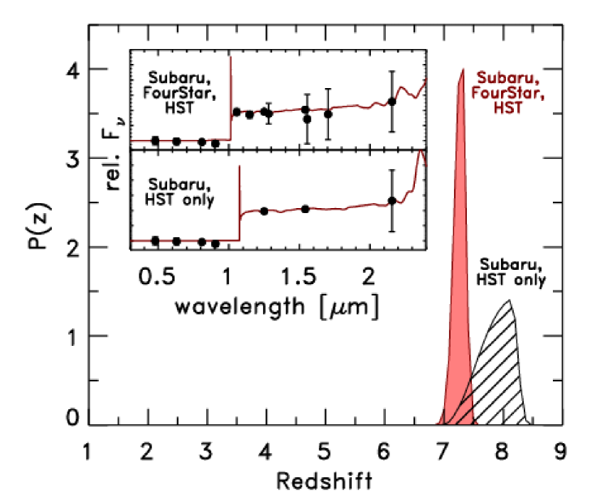
Figure 10.— Comparison of photometric redshift probability distribution of the brightest object (zF13965) using only broad-band photometry (HST+Subaru+IRAC: hashed region), and adding medium-band filters (FourStar + HST+Subaru +IRAC bands : filled red region). The photometric redshifts using the FourStar medium-band filters prefers a lower as well as narrower redshift range.

5.1.1 Photometric Redshift Distribution

Figure 10 shows the photometric redshift probability distribution for the brightest object. For the brightest object (zF13965), the photometric redshifts derived for the HST+Subaru bands tend to be higher with $z_{\rm phot}$=8.11${}^{+0.45}_{-1.06}$, while inclusion of medium-band photometry lowers the photometric redshift to $z_{\rm phot}$=7.24${}^{+0.38}_{-0.25}$ (where the error bars are all 99% confidence; Figure 10). This is also true for the 2nd brightest object (zF25035), with $z_{\rm phot}$=7.66${}^{+0.77}_{-0.57}$ and $z_{\rm phot}$=7.16${}^{+0.35}_{-0.19}$ when derived using broad-band photometry alone, and then adding medium-band filters, respectively. The addition of medium-band photometry lowers the median redshift because of the J₁ filter, which better constrains the Lyman-break. Surveys using a Y-band near-IR filter may expect similar photometric redshifts. Including the medium-band filters, the photometric redshift probability distribution functions favor lower redshift solutions, with a narrower range of favored redshfits. We fit the stellar-population models to the measured photometry over a range of redshift spanned by these probability distribution functions, and we marginalize over these properties when determining constraints on stellar population parameters.

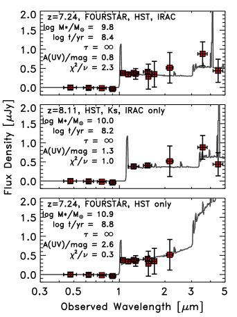
Figure 11.— Comparison of SED of our brightest candidate (zF13965) using all bands (top panel: HST+Subaru + FourStar medium-band +IRAC) and excluding medium-band photometry (middle panel: HST+Subaru +IRAC bands). The SED model assumes 0.2$\rm Z_{\odot}$ metallicity, a Chabrier IMF, the Bruzual & Charlot 2003 model, and include nebular emission lines. The lower panel shows best-fit SED without IRAC bands. Adding FourStar medium-band filters improves the constraints on the photometric redshift and other physical properties, while exclusion of IRAC bands yields poorest constraints.

5.1.2 Best-fit SED

Figure 11 shows the best-fit model spectrum with and without the FourStar medium-band filters for our brightest $z\sim 7$ LBG. The top panel shows the best-fit model spectrum using FourStar medium-band filters, HST  and visible bands while the middle panel shows the best-fit SED without the FourStar medium-band data. The bottom panel shows the effects when the IRAC bands are excluded. In all three cases, we use the photometric redshifts obtained from EAZY, using respective bands only. The behavior of the best-fit SEDs for the second brightest $z\sim 7$ galaxy are very similar.

5.1.3 UV Spectral Slope

The UV continuum light is sensitive to dust absorption and its slope provides a good tracer of the dust attenuation for star-forming galaxies as the two are well correlated in UV-luminous, star-forming galaxies from $z\sim 0$ to $\sim 3$ (Meurer et al., 1995, 1997, 1999; Daddi et al., 2004; Burgarella et al., 2005; Laird et al., 2005; Reddy et al., 2006; Dale et al., 2007; Treyer et al., 2007; Salim et al., 2007).

Recently, Finkelstein et al. (2011) measured UV spectral slopes of $z\sim 7$ galaxies by directly fitting the best-fit SED with a power-law. We followed a similar procedure to measure $\beta$ by fitting a power-law to the best-fit SED in the the rest-frame wavelength range $1250\leq\lambda\leq 2600$ Å  (Calzetti et al., 1994).

For the brightest LBG in our sample (zF13965), with this method we find $\beta$=-1.88$\pm 0.1$ using the HST bands while adding the medium-band photometry gives a steeper value of $\beta$=-2.08$\pm 0.1$ (see Table 3). For the 2nd brightest LBG (zF25035), we find a similar trend in $\beta$ with a shallower slope, $\beta=-1.29$$\pm 0.05$ using HST  broad-band photometry and a steeper $\beta=-1.44$$\pm 0.12$ when adding medium-band photometry. For both galaxies, our analyses favor steeper (i.e., bluer) UV spectral slopes when the medium-band photometry are included.

The UV slope measured for both objects are between $\beta$=-1.2 to $\beta$=-2.1, within the range seen in other studies at $z\sim 7$. Finkelstein et al (2011) found a median value of $\beta$=-2.1 for galaxies with $\rm M_{UV}=-20.6$. Similarly, Dunlop et al (2012) found an average value of $\beta$=-2 for bright $z\sim 7$  galaxies with $\rm M_{UV}=-20.5$.

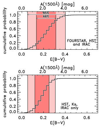
Figure 12.— Cumulative probability distribution of E(B-V), for the $2^{nd}$ brightest candidate (zF25035), using broad-band photometry alone (top panel), while the bottom panel includes medium-band photometry. While the median E(B-V)=0.2 are nearly same for both, the E(B-V) derived using medium-band filters allows a wider distribution compared to the the distribution obtained using broad-band photometry alone.

Table 3Physical properties derived from spectral energy distribution fitting for the two brightest LBG candidates (zF13965 & zF25035).

ID	Filters	$z_{\rm phot}$	$\beta$	E(B-V)	Log Stellar	Stellar age	Best-fit
					mass $\rm M_{\odot}$	Myr	$\tau$ (Gyr)
zF13965	HST+Subaru+IRAC+FourStar	7.24${}^{+0.38}_{-0.25}$	-2.08${}^{+0.10}_{-0.10}$	0.09${}^{+0.06}_{-0.05}$	9.8${}^{+0.2}_{-0.2}$	251	100
	HST+Subaru+IRAC	8.11${}^{+0.45}_{-1.06}$	-1.88${}^{+0.10}_{-0.10}$	0.01${}^{+0.20}_{-0.01}$	10.0${}^{+0.2}_{-0.3}$	159	100
	HST+Subaru++no IRAC+FourStar	7.24${}^{+0.38}_{-0.25}$	-1.17${}^{+0.05}_{-0.05}$	-	11.3${}^{+0.5}_{-0.7}$	630	100
1-7 zF25035	HST+Subaru+FourStar	7.16${}^{+0.35}_{-0.19}$	-1.44${}^{+0.12}_{-0.12}$	0.22${}^{+0.09}_{-0.09}$	10.4${}^{+0.3}_{-0.4}$	321	100
	HST+Subaru	7.66${}^{+0.77}_{-0.57}$	-1.29${}^{+0.05}_{-0.05}$	0.24${}^{+0.07}_{-0.20}$	10.2${}^{+0.3}_{-0.3}$	640	100
	HST+Subaru++no IRAC+FourStar	7.16${}^{+0.35}_{-0.19}$	-1.52${}^{+0.10}_{-0.10}$	-	10.4${}^{+0.5}_{-0.4}$	640	100

• Median value. Errors indicate upper and lower 68% values.

• We report the best-fit ages from the spectral-energy distribution modeling only, as the age constraints depend strongly on the assumed star-formation history.

5.1.4 Constraints on Dust Attenuation from SED Fitting

Finkelstein et al. (2010) found the best-fit A(V)=0 $-$ 1.5 for a sample of LBGs at $z\sim 7$  obtained from the HST WFC3 in the HUDF field, while Labbé et al. (2010) found A(V)=0 for a stacked sample of $z\sim 7$  LBGs, also obtained from the HST. Figure 12 shows the cumulative probability distribution of the dust content E(B-V) for our 2nd brightest object (zF25035) from the SED fitting. The shaded regions show 68% and 95% confidence regions. The top panel shows E(B-V) with broad-band +FourStar photometry, while the bottom panel shows the probability when including broad-band photometry alone (Table 3).

While the best-fit model, with and without the medium-bands, yield similar range of E(B-V), the probability distribution with the medium-bands spans a wider range with a median E(B-V) $=$ 0.22, slightly lower compared with the median E(B-V) that excludes the medium-band filters. For the brightest LBG (zF13965), median E(B-V)=0.01 and E(B-V)=0.09 with and without FourStar bands respectively. For the reasons described above, the FourStar bands provide a more robust constraint on the physical properties of galaxies owing to their higher spectral resolution.

5.1.5 Stellar Mass and Age

Bowler et al. (2012) found that LBGs at $z\sim 7$  with magnitudes in the range of our two most-luminous sources ($J\sim 25$ mag) have stellar mass $\sim 5\times 10^{9}$$\rm M_{\odot}$. For fainter magnitudes, depending on the range of extinction, the estimated stellar masses range from $3\times 10^{7}$ - $1\times 10^{10}$$\rm M_{\odot}$(Finkelstein et al., 2010; Labbé et al., 2010).

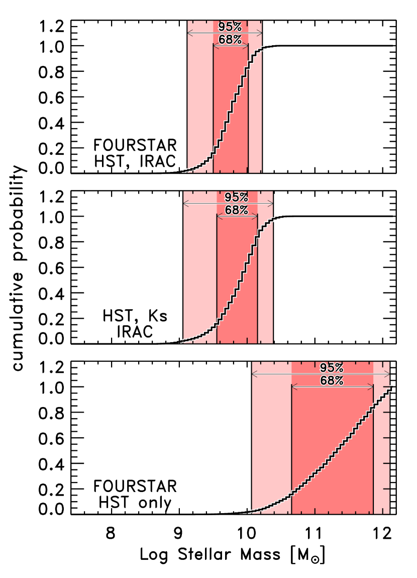
Figure 13.— Cumulative distribution of stellar mass for the most luminous $z\sim 7$  LBG (zF13965) with all bands included (top panel), excluding FourStar medium-band filters (middle panel), and excluding IRAC bands (lower panel). The addition of medium-band photometry shifts the stellar mass distribution to lower values (from $1\times 10^{10}$ $\rm M_{\odot}$ to $6.3\times 10^{9}$ $\rm M_{\odot}$) because it better measures the spectrum of the galaxy. Removing the IRAC data allows for a large range of stellar-population parameters, including older age models, which greatly extends the range of stellar masses to higher values.

For our brightest object (zF13965), the favored range of stellar mass shifts to lower values after including the medium-band filters, with the most likely median mass decreasing by a factor of 1.5. As can be seen in Figure 13, the probability distribution is narrower with median mass $6.3\times 10^{9}$ $\rm M_{\odot}$ when the medium-band filters are included; the absence of the FourStar medium-band photometry shifts the masses to higher values (median mass $=1\times 10^{10}$ $\rm M_{\odot}$). On the other hand, for the second brightest object (zF25035), the median mass is higher ($2.5\times 10^{10}$  $\rm M_{\odot}$) when medium-band filters are included.

Figure 13 (bottom panel) shows the constraints if we remove the IRAC bands. In this case, the allowed range of stellar population parameters that fits the rest-frame UV extends to models with very old ages and high mass-to-light ratios, and the fits are no longer able to exclude these possibilities. Thus, for the brightest object, the IRAC photometry is essential to better constrain the best-fit stellar masses. For the second object however, the presence of IRAC bands does not change the derived stellar mass (Table 3). A likely reason for this is that in our models the redshifted [OIII] line flux falls in the 4.5$\mu$m band over the photometric redshift range. This boosts the flux in the model, and requires lower stellar masses.

The stellar ages for the two brightest objects range from 250 to 640 Myr, albeit with large uncertainties which depend on the assumed star-formation history. We can however estimate the timescale over which the stellar mass doubles. Because the best-fit $\tau$ (Table 3) for both objects is large (100 Gyr), the timescale is simply stellar mass/SFR. This yields a timescale of about 150 Myr to double the stellar mass.

In summary, using broad-band photometry alone, broadens the photometric redshift range compared to the result when the medium-band data are included. This is expected as the medium-band filters more accurately isolate the location of the Lyman-break. In addition, currently there are no broad-band filters corresponding to the central wavelengths of some of the FourStar medium-band filters (see Figure 1).

While our comparison is based on only two $z\sim 7$  dropout galaxies, they are at the upper luminosity (and stellar mass) range of galaxies at this redshift. For our small sample, adding the medium-band photometry to the SED fitting yield more accurate constraints on the physical properties of the $z\sim 7$  galaxies compared to using broad-band photometry alone. To generalize these conclusions to the $z\sim 7$  galaxy population will however require larger samples with deep medium-band imaging.

5.1.6 Effect of Lyman-$\alpha\;$ Line and J₁ Filter on SED Fitting

We further investigated the presence of a Lyman-$\alpha\;$ line and the effect of the J₁ filter on the derived physical properties of our bright LBGs. To do this, we obtained the best-fit SED (section 5.1) by first including no Lyman-$\alpha\;$  emission and then by excluding the J₁  filter. Excluding the J₁ filter or absence of a Lyman-$\alpha\;$ flux results in essentially the same values as that for broad-band only derived parameters. This reinforces the idea that we need Lyman-$\alpha\;$ equivalent width measurements to understand (1) the dust extinction and (2) the stellar masses, especially for galaxies with Lyman-$\alpha\;$ emission line.

5.1.7 Lyman-$\alpha\;$Equivalent Width

In principle, the Lyman-$\alpha\;$  equivalent width $W$ provides a proxy to the star-formation rate in the galaxy, and defined as $W\equiv F_{\rm line}/F_{\lambda}^{c}$, where $F_{\rm line}$ is the total line flux ($\rm erg\;s^{-1}\;cm^{-2}$) and $F_{\lambda}^{c}$ is the continuum flux density ($\rm erg\;s^{-1}\;cm^{-2}\;\AA^{-1}$). If our $z\sim 7$  LBG candidates have Lyman-$\alpha\;$ line, it will contribute a flux excess in the J₁ filter, thereby decreasing (i.e., making brighter) the J₁  magnitude (Papovich et al., 2001);

$$\Delta m\simeq-2.5\log\left[1+\frac{W_{0}(1+z)}{\Delta\lambda}\right],$$ (8)

where $W_{0}$ is the rest-frame Lyman-$\alpha\;$ equivalent width and $\Delta\lambda$ is the J₁ filter width.

To measure $\Delta m$, we followed two different methods to take advantage of the presence of J₁ filter. In the $\rm 1^{st}$ method, we first obtain the best-fit SED using all photometry and including the emission line (see Section 5.1). We then use this best-fit SED, but remove the emission line, and measure the bandpass J₁ magnitude. This magnitude compared with the observed J₁ magnitude yields $\Delta m$. In the $\rm 2^{nd}$ method, instead of removing the emission line, we obtain the best-fit excluding the J₁ filter and compare the observed J₁ magnitude with the synthesized J₁ magnitude to get $\Delta m$. We calculate the rest-frame equivalent widths using Equation 8 for our two brightest $z\sim 7$  LBG candidates (Table 4). Using these $W_{0}$, we calculate the Lyman-$\alpha\;$ line flux:

$$F_{\rm line}=F_{\lambda}^{c}\;W_{0}\;(1+z).$$ (9)

Table 4Estimated rest-frame Lyman-$\alpha\;$ equivalent widths and Lyman-$\alpha\;$ line fluxes for the two brightest $z\sim 7$  LBG candidates.

ID		EW0		Lyman-$\alpha\;$ flux
		(Å)		$(10^{-17}$ $\rm erg\;s^{-1}\;cm^{-2}$)
Method 1
zF13965		16.5${}^{+15.3}_{-15.3}$		1.15${}^{+1.07}_{-1.07}$
zF25035		26.2${}^{+16.1}_{-16.1}$		1.07${}^{+0.66}_{-0.66}$
Method 2
zF13965		-1.0${}^{+12.6}_{-12.6}$		0.0${}^{+1.0}_{-1.0}$
zF25035		13.5${}^{+14.3}_{-14.3}$		0.6${}^{+0.66}_{-0.66}$

Table 4 shows the estimated Lyman-$\alpha\;$ EWs and line fluxes, obtained from both methods, for the the two brightest $z\sim 7$  LBG candidates. The Lyman-$\alpha\;$ EWs are smaller when the J₁ filter is excluded ( $\rm 2^{nd}$ method). On the other hand, the Lyman-$\alpha\;$ fluxes obtained from the $\rm 1^{st}$ method are similar to the recent observations of spectroscopically confirmed LBGs at $z$=7.008 and $z=$7.109, with line fluxes 1.62 $\times 10^{-17}$ and 1.21 $\times 10^{-17}$ $\rm erg\;s^{-1}\;cm^{-2}$, respectively (Vanzella et al., 2011). These line fluxes are accessible to deep spectroscopy with $>$8m telescopes, and thus these two candidates provide good targets for future spectroscopic followup.

5.2. Specific Star Formation Rate

The specific star formation rate, sSFR (SFR/$M_{\star}$) provides a way to quantify the evolution of mass build-up given a certain SFR. Many observations suggest that the sSFR is nearly constant from $z\sim 7$ to $z\sim 4$ (Stark et al., 2009; González et al., 2010; Bouwens et al., 2011). This implies that the SFR increase from high-redshifts to low-redshifts, in conflict with the general assumption of constant or declining SFH. However, recent studies (e.g., Stark et al., 2012; Schaerer & de Barros, 2012) suggest that there is a stronger evolution in the sSFR from low-redshift to high-redshifts, than suggested by previous studies. Thus, to resolve this uncertainty among different studies, large samples of high-redshift galaxies are needed.

Here we estimate the sSFR for the two brightest galaxies in our $z\sim 7$  sample using the more accurate physical parameters derived from the fits to the FourStar medium-band + HST + IRAC data. We derived the SFRs using the best-fit SEDs: for the brightest LBG (zF13965), the median SFR=77.6${}^{+62}_{-42}$ $\rm M_{\odot}$ yr^-1, much smaller compared with the 2nd brightest LBG (zF25035) with median SFR=285.7${}^{+346}_{-179}$ $\rm M_{\odot}$ yr^-1(Table 5).

Our derived sSFR $\sim$ 13  Gyr^-1 for the two brightest $z\sim 7$  LBG candidate is slightly higher compared with the values derived for lower luminosity (and lower mass) galaxies at $z\sim 7$, which implies a nearly constant sSFR from $z\sim 7$ to $z\sim 4$ (e.g., Reddy et al., 2012) for galaxies over approximately a decade in stellar mass ($2\times 10^{9}$ $\rm M_{\odot}$ to $2\times 10^{10}$ $\rm M_{\odot}$). These sSFRs favors the idea that galaxies at these epochs have rising star-formation histories such that the sSFR is nearly independent of mass at a fixed redshift (e.g. Papovich et al., 2011). Models with constant or declining SFHs would imply decreasing sSFR with increasing mass at fixed redshift, which is disfavored.

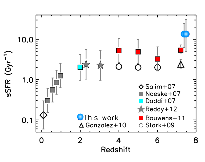
Figure 14.— The redshift evolution of the specific SFR. Blue filled circles represent the two brightest galaxies from FourStar observations. Open diamond, open circles, and open triangle represent data from Salim et al. (2007), Stark et al. (2009), and González et al. (2010) respectively while filled symbols- grey squares, cyan square, stars, and red squares show observations from Noeske et al. (2007), Daddi et al. (2007), Reddy et al. (2012), and Bouwens et al. (2011) respectively. These galaxies have stellar masses $\rm M_{\star}=(1-2)\times 10^{10}$ $\rm M_{\odot}$. The error bars on the FourStar observations are the uncertainties in the estimated stellar mass obtained from the best-fit SED. The sSFR remains nearly constant over 1 Gyr period from $z=8$ to $z=4$, which favors the idea of rising star-formation history with increasing stellar mass (Papovich et al., 2011).

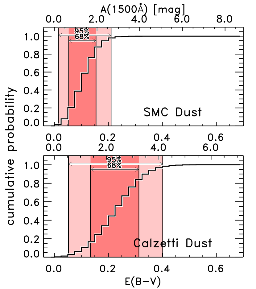
Figure 15.— Comparison of dust extinction derived from the best-fit SED using Calzetti and SMC dust extinction law. Here we have shown the dust extinction of the 2nd brightest LBG (zF25035) as this object yields significantly different extinctions for SMC and Calzetti dust extinction law, compared with the brightest LBG (zF13965). The SMC-like law yields a median E(B-V)=0.1, a value much smaller compared with median E(B-V)=0.22 obtained using the Calzetti dust extinction law.

Table 5Comparison of derived physical parameters from the best-fit SEDs using Calzetti and SMC dust extinction laws for the two brightest LBGs.

	zF13965	zF25035
$\chi^{2}/\nu$	2.3   [1.8]	0.7   [0.7]
Log Mass($\rm M_{\odot}$)	9.8${}^{+0.2}_{-0.2}$   [9.6${}^{+0.3}_{-0.4}$]	10.3${}^{+0.3}_{-0.4}$   [9.8${}^{+0.3}_{-0.4}$]
E(B-V)	0.09${}^{+0.06}_{-0.05}$   [0.05${}^{+0.03}_{-0.03}$]	0.22${}^{+0.09}_{-0.09}$   [0.1${}^{+0.05}_{-0.05}$]
SFR($\rm M_{\odot}$yr-1)	77.6${}^{+62.3}_{-42.5}$   [57.8${}^{+32.7}_{-24.4}$]	285.7${}^{+346.6}_{-179.6}$ [62.7${}^{+75.7}_{-33.6}$]
sSFR(Gyr-1)	13.5 ${}^{+1.8}_{-2.2}$ [13.5 ${}^{+2.0}_{-2.7}$]	13.5 ${}^{+2.3}_{-2.7}$ [10.7 ${}^{+2.3}_{-2.6}$]

• Values in square brackets are derived using SMC extinction law.

5.3. Comparison Using Calzetti & SMC Dust Extinction Laws

To compare the effect of different extinction laws on the derived physical properties of $z\sim 7$  LBGs, we derived the best-fit SEDs (see Section 5.1.2) and physical properties of the two brightest $z\sim 7$  LBG candidates using Calzetti and SMC dust extinction laws.

For the brightest LBG (zF13965), all derived parameters (stellar mass, age, and $\chi^{2}$) using SMC dust extinction law decrease except for the dust extinction (see Table 5). For the 2nd brightest LBG (zF25035), stellar mass, extinction and $\chi^{2}$ either decrease or remain unchanged except for the stellar age. A major difference among these two LBGs is that the dust extinction for zF25035 is significantly reduced ($\rm A_{UV}$=0.9) when using the SMC extinction law (see Fig. 15). This smaller extinction value also gives rise to the lower SFR compared with the Calzetti dust extinction-derived SFR. This demonstrates that the assumption of the extinction law affects the interpretation of the dust content in high-redshift galaxies. In particular, the SMC-type law - which may be more applicable in these distant galaxies (Oesch et al., 2012b) - reduces the implied dust content compared to a Calzetti-type law for low-redshift luminous starburst galaxies.

6. Summary & Conclusions

We have obtained a sample of $z\sim 7$  galaxies from a deep near-IR survey (zFourGE ) using medium-band filters for the first time. We define a color-color selection criteria for the near-IR medium-band filters, which cleanly isolate $z\sim 7$  LBG candidates from brown dwarf stars and low-redshift galaxies. Using our criteria we have identified three robust $z\sim 7$  candidate LBGs in a survey area of about 155 arcmin² in the COSMOS field, which has very deep publically available data. The availability of near-IR medium-band and broad-band photometry allowed us to compare the derived physical properties of high-redshift galaxies and how these properties are influenced by the choice of filter widths. Our principal findings are summarized below.

Stars vs compact galaxies$-$ While the contamination from nearby T-dwarf stars is a serious concern for dropout-selected galaxies, especially when using the ground-based broad-band photometry, the FourStar medium-band filters allow us to cleanly distinguish between nearby dwarf stars and high-redshift galaxies that are relatively compact.

One of the three $z\sim 7$  LBGs in our sample (zF25035) is very compact and indistinguishable from a point source at ground-based resolution (and possibly unresolved even by HST). Our ability to distinguish this object from cool stars is possible only due to the availability of multiwavelength medium-band photometry. Moreover, this demonstrates that there exists a population of very compact galaxies at $z\sim 7$.

Bright end of the $z\sim 7$  UV luminosty function$-$ Using the number density of $z\sim 7$  galaxies obtained using dropout technique and corrected for incompleteness, the rest-frame stepwise UV luminosity function at $z\sim 7$  shows a moderate evolution from $z\sim 5$. The number density of bright LBGs ($M_{UV}$$\sim$-21.5) increases by a factor of 4 from $z\sim 7$  to $z\sim 5$ albeit with large error bars. This is consistent with other ground-based studies but implies lesser evolution compared to the factor of 10 increase implied by some HST-based studies.

Physical properties of $z\sim 7$  galaxies$-$ In general, the presence of medium-band photometry yield tighter constraints on the photometric redshifts and improved physical constraints on the stellar population parameters of these galaxies.

1. For our two brightest LBGs, the best-fit SED model with broad-band + medium-band photometry yields lower photometric redshifts, and much tighter redshift probability distribution compared to the $z_{\rm phot}$$\sim$8 derived using only broad-band photometry (Figure  10). This is also true for our 2nd brightest object.

2. For both objects, the UV spectral slope $\beta$ tends to be shallower when derived using broad-band photometry alone. For the brightest object, $\beta$ changes from -1.88 to -2.08 when FourStar medium-band photometry is included.

3. The SED modeling prefers a lower dust attenuation with median E(B-V)=$0.01$ for broad-band photometry, while it increases to median E(B-V)=$0.09$ when including medium-band photometry. The FourStar bands allow for redder UV colors which increases the range of permitted values for E(B-V). Comparing the above values, derived using the Calzetti dust law, with the E(B-V) derived using SMC-like dust law, we find that the probability distribution from the latter case is much narrower and shifts towards lower values (Figure 15).

4. Including the FourStar medium-band filters, the SED modeling yields narrower probability distribution for stellar mass for the two most luminous objects in our sample. We argue that adding additional bands shifts the allowed regions of the stellar-population parameter space, improving our physical understanding of the galaxies. We find that the presence of IRAC photometry is also important to better constrain the best-fit stellar masses.

5. We predict the Lyman-$\alpha\;$ equivalent widths and line fluxes of the two brightest candidates and find that the presence of Lyman-$\alpha\;$ line influences the derived physical properties of $z\sim 7$  candidates. The estimated rest-frame equivalent widths (17 and 26 Å) make these two objects good targets for future spectroscopic followup.

6. The sSFRs for the two most luminous galaxies are slightly larger compared with other lower mass galaxies at $z\sim 7$. This favors the ideal that the SFR increases with increasing stellar mass at this redshift.

While it is early to reach robust conclusions about the effect of medium-band photometry on the derived properties of $z\sim 7$  galaxies, medium-band filters will likely provide better constraints on the physical properties, due to their narrower redshift probability distributions, compared to the broad-band photometry. If this is indeed true, in the absence of spectroscopic redshifts, multiwavelength medium-band photometry will provide the best constraints on the physical properties of $z\sim 7$  galaxies.

References

- Adelberger et al. (2004) Adelberger, K. L., Steidel, C. C., Shapley, A. E., et al. 2004, ApJ, 607, 226
- Bertin & Arnouts (1996) Bertin, E., & Arnouts, S. 1996, A&AS, 117, 393
- Bertin et al. (2002) Bertin, E., Mellier, Y., Radovich, M., et al. 2002, Astronomical Data Analysis Software and Systems XI, 281, 228
- Bouwens et al. (2006) Bouwens, R. J., Illingworth, G. D., Blakeslee, J. P., & Franx, M. 2006, ApJ, 653, 53
- Bouwens et al. (2007) Bouwens, R. J., Illingworth, G. D., Franx, M., & Ford, H. 2007, ApJ, 670, 928
- Bouwens et al. (2008) Bouwens, R. J., Illingworth, G. D., Franx, M., & Ford, H. 2008, ApJ, 686, 230
- Bouwens et al. (2009a) Bouwens, R. J., Illingworth, G. D., Franx, M., et al. 2009, ApJ, 705, 936
- Bouwens et al. (2010) Bouwens, R. J., Illingworth, G. D., Oesch, P. A., et al. 2010, ApJ, 708, L69
- Bouwens et al. (2011) Bouwens, R. J., Illingworth, G. D., Labbe, I., et al. 2011, Nature, 469, 504
- Bouwens et al. (2012) Bouwens, R. J., Illingworth, G. D., Oesch, P. A., et al. 2012, ApJ, 752, L5
- Bowler et al. (2012) Bowler, R. A. A., Dunlop, J. S., McLure, R. J., et al. 2012, arXiv:1205.4270
- Bradley et al. (2012) Bradley, L. D., Bouwens, R. J., Zitrin, A., et al. 2012, ApJ, 747, 3
- Brammer et al. (2008) Brammer, G. B., van Dokkum, P. G., & Coppi, P. 2008, ApJ, 686, 1503
- Brammer et al. (2011) Brammer, G. B., Whitaker, K. E., van Dokkum, P. G., et al. 2011, ApJ, 739, 24
- Bruzual & Charlot (2003) Bruzual, G., & Charlot, S. 2003, MNRAS, 344, 1000
- Burgarella et al. (2005) Burgarella, D., Buat, V., & Iglesias-Páramo, J. 2005, MNRAS, 360, 1413
- Burgasser et al. (2006) Burgasser, A. J., Geballe, T. R., Leggett, S. K., Kirkpatrick, J. D., & Golimowski, D. A. 2006, ApJ, 637, 1067
- Calzetti et al. (1994) Calzetti, D., Kinney, A. L., & Storchi-Bergmann, T. 1994, ApJ, 429, 582
- Calzetti (1997) Calzetti, D. 1997, AJ, 113, 162
- Calzetti et al. (2000) Calzetti, D., Armus, L., Bohlin, R. C., et al. 2000, ApJ, 533, 682
- Capak et al. (2011) Capak, P., Mobasher, B., Scoville, N. Z., et al. 2011, ApJ, 730, 68
- Castellano et al. (2010) Castellano, M., Fontana, A., Boutsia, K., et al. 2010, A&A, 511, A20
- Daddi et al. (2004) Daddi, E., Cimatti, A., Renzini, A., et al. 2004, ApJ, 617, 746
- Daddi et al. (2007) Daddi, E., Dickinson, M., Morrison, G., et al. 2007, ApJ, 670, 156
- Dale et al. (2007) Dale, D. A., Gil de Paz, A., Gordon, K. D., et al. 2007, ApJ, 655, 863
- Dickinson et al. (2004) Dickinson, M., Stern, D., Giavalisco, M., et al. 2004, ApJ, 600, L99
- Dickinson et al. (2003) Dickinson, M., Papovich, C., Ferguson, H. C., & Budavári, T. 2003, ApJ, 587, 25
- Erb et al. (2006) Erb, D. K., Shapley, A. E., Pettini, M., et al. 2006, ApJ, 644, 813
- Fan et al. (2002) Fan, X., Narayanan, V. K., Strauss, M. A., et al. 2002, AJ, 123, 1247
- Fazio et al. (2004) Fazio, G. G., Hora, J. L., Allen, L. E., et al. 2004, ApJS, 154, 10
- Finkelstein et al. (2010) Finkelstein, S. L., Papovich, C., Giavalisco, M., et al. 2010, ApJ, 719, 1250
- Finkelstein et al. (2011) Finkelstein, S. L., Cohen, S. H., Moustakas, J., et al. 2011, ApJ, 733, 117
- Finkelstein et al. (2012) Finkelstein, S. L., Papovich, C., Ryan, R. E., Jr., et al. 2012, arXiv:1206.0735
- Fontana et al. (2006) Fontana, A., Salimbeni, S., Grazian, A., et al. 2006, A&A, 459, 745
- Giavalisco et al. (2004) Giavalisco, M., Ferguson, H. C., Koekemoer, A. M., et al. 2004, ApJ, 600, L93
- González et al. (2010) González, V., Labbé, I., Bouwens, R. J., et al. 2010, ApJ, 713, 115
- Grazian et al. (2011) Grazian, A., Castellano, M., Koekemoer, A. M., et al. 2011, A&A, 532, A33
- Grogin et al. (2011) Grogin, N. A., Kocevski, D. D., Faber, S. M., et al. 2011, ApJS, 197, 35
- Hathi et al. (2012) Hathi, N. P., Mobasher, B., Capak, P., Wang, W.-H., & Ferguson, H. C. 2012, ApJ, 757, 43
- Hibon et al. (2010) Hibon, P., Cuby, J.-G., Willis, J., et al. 2010, A&A, 515, A97
- Iye et al. (2006) Iye, M., Ota, K., Kashikawa, N., et al. 2006, Nature, 443, 186
- Kennicutt (1998) Kennicutt, R. C., Jr. 1998, ARA&A, 36, 189
- Koekemoer et al. (2011) Koekemoer, A. M., Faber, S. M., Ferguson, H. C., et al. 2011, ApJS, 197, 36
- Komatsu et al. (2011) Komatsu, E., Smith, K. M., Dunkley, J., et al. 2011, ApJS, 192, 18
- Kashikawa et al. (2006) Kashikawa, N., Shimasaku, K., Malkan, M. A., et al. 2006, ApJ, 648, 7
- Krug et al. (2012) Krug, H. B., Veilleux, S., Tilvi, V., et al. 2012, ApJ, 745, 122
- Labbé et al. (2007) Labbé, I., Franx, M., Rudnick, G., et al. 2007, ApJ, 665, 944
- Labbé et al. (2003) Labbé, I., Franx, M., Rudnick, G., et al. 2003, AJ, 125, 1107
- Labbé et al. (2010) Labbé, I., González, V., Bouwens, R. J., et al. 2010, ApJ, 716, L103
- Laird et al. (2005) Laird, E. S., Nandra, K., Adelberger, K. L., Steidel, C. C., & Reddy, N. A. 2005, MNRAS, 359, 47
- Madau (1995) Madau, P. 1995, ApJ, 441, 18
- Malhotra & Rhoads (2002) Malhotra, S., & Rhoads, J. E. 2002, ApJ, 565, L71
- McLure et al. (2010) McLure, R. J., Dunlop, J. S., Cirasuolo, M., et al. 2010, MNRAS, 403, 960
- Meiksin (2006) Meiksin, A. 2006, MNRAS, 365, 807
- Meurer et al. (1995) Meurer, G. R., Heckman, T. M., Leitherer, C., et al. 1995, AJ, 110, 2665
- Meurer et al. (1997) Meurer, G. R., Heckman, T. M., Lehnert, M. D., Leitherer, C., & Lowenthal, J. 1997, AJ, 114, 54
- Meurer et al. (1999) Meurer, G. R., Heckman, T. M., & Calzetti, D. 1999, ApJ, 521, 64
- Noeske et al. (2007) Noeske, K. G., Faber, S. M., Weiner, B. J., et al. 2007, ApJ, 660, L47
- Oesch et al. (2010) Oesch, P. A., Bouwens, R. J., Illingworth, G. D., et al. 2010, ApJ, 709, L16
- Ono et al. (2012) Ono, Y., Ouchi, M., Mobasher, B., et al. 2012, ApJ, 744, 83
- Ouchi et al. (2009) Ouchi, M., Mobasher, B., Shimasaku, K., et al. 2009, ApJ, 706, 1136
- Oesch et al. (2012) Oesch, P. A., Bouwens, R. J., Illingworth, G. D., et al. 2012, ApJ, 745, 110
- Oesch et al. (2012b) Oesch, P. A., Labbe, I., Bouwens, R. J., et al. 2012, arXiv:1211.1010
- Ouchi et al. (2004) Ouchi, M., Shimasaku, K., Okamura, S., et al. 2004, ApJ, 611, 660
- Overzier et al. (2009) Overzier, R. A., Shu, X., Zheng, W., et al. 2009, ApJ, 704, 548
- Ouchi et al. (2009b) Ouchi, M., Ono, Y., Egami, E., et al. 2009, ApJ, 696, 1164
- Papaderos et al. (2002) Papaderos, P., Izotov, Y. I., Thuan, T. X., et al. 2002, A&A, 393, 461
- Papovich et al. (2001) Papovich, C., Dickinson, M., & Ferguson, H. C. 2001, ApJ, 559, 620
- Papovich et al. (2004) Papovich, C., Dickinson, M., Ferguson, H. C., et al. 2004, ApJ, 600, L111
- Papovich et al. (2011) Papovich, C., Finkelstein, S. L., Ferguson, H. C., Lotz, J. M., & Giavalisco, M. 2011, MNRAS, 412, 1123
- Pei (1992) Pei, Y. C. 1992, ApJ, 395, 130
- Peng et al. (2002) Peng, C. Y., Ho, L. C., Impey, C. D., & Rix, H.-W. 2002, AJ, 124, 266
- Pustilnik et al. (2004) Pustilnik, S. A., Pramskij, A. G., & Kniazev, A. Y. 2004, A&A, 425, 51
- Reddy & Steidel (2004) Reddy, N. A., & Steidel, C. C. 2004, ApJ, 603, L13
- Reddy et al. (2005) Reddy, N. A., Erb, D. K., Steidel, C. C., et al. 2005, ApJ, 633, 748
- Reddy et al. (2006) Reddy, N. A., Steidel, C. C., Erb, D. K., Shapley, A. E., & Pettini, M. 2006, ApJ, 653, 1004
- Reddy et al. (2008) Reddy, N. A., Steidel, C. C., Pettini, M., et al. 2008, ApJS, 175, 48
- Reddy & Steidel (2009) Reddy, N. A., & Steidel, C. C. 2009, ApJ, 692, 778
- Reddy et al. (2012) Reddy, N. A., Pettini, M., Steidel, C. C., et al. 2012, ApJ, 754, 25
- Rhoads et al. (2005) Rhoads, J. E., Panagia, N., Windhorst, R. A., et al. 2005, ApJ, 621, 582
- Rieke et al. (2004) Rieke, G. H., Young, E. T., Engelbracht, C. W., et al. 2004, ApJS, 154, 25
- Salim et al. (2007) Salim, S., Rich, R. M., Charlot, S., et al. 2007, ApJS, 173, 267
- Shapley et al. (2001) Shapley, A. E., Steidel, C. C., Adelberger, K. L., et al. 2001, ApJ, 562, 95
- Shapley et al. (2005) Shapley, A. E., Steidel, C. C., Erb, D. K., et al. 2005, ApJ, 626, 698
- Stanway et al. (2003) Stanway, E. R., Bunker, A. J., & McMahon, R. G. 2003, MNRAS, 342, 439
- Shimasaku et al. (2005) Shimasaku, K., Ouchi, M., Furusawa, H., et al. 2005, PASJ, 57, 447
- Sawicki & Yee (1998) Sawicki, M., & Yee, H. K. C. 1998, AJ, 115, 1329
- Salvaterra et al. (2011) Salvaterra, R., Ferrara, A., & Dayal, P. 2011, MNRAS, 414, 847
- Schenker et al. (2012) Schenker, M. A., Stark, D. P., Ellis, R. S., et al. 2012, ApJ, 744, 179
- Schaerer & de Barros (2009) Schaerer, D., & de Barros, S. 2009, A&A, 502, 423
- Schaerer et al. (2011) Schaerer, D., de Barros, S., & Stark, D. P. 2011, A&A, 536, A72
- Schaerer & de Barros (2012) Schaerer, D., & de Barros, S. 2012, IAU Symposium, 284, 20
- Spitler et al. (2012) Spitler, L. R., Labbé, I., Glazebrook, K., et al. 2012, ApJ, 748, L21
- Scoville et al. (2007) Scoville, N., Aussel, H., Brusa, M., et al. 2007, ApJS, 172, 1
- Stark et al. (2009) Stark, D. P., Ellis, R. S., Bunker, A., et al. 2009, ApJ, 697, 1493
- Stark et al. (2012) Stark, D. P., Schenker, M. A., Ellis, R. S., et al. 2012, arXiv:1208.3529
- Steidel et al. (1999) Steidel, C. C., Adelberger, K. L., Giavalisco, M., Dickinson, M., & Pettini, M. 1999, ApJ, 519, 1
- Steidel et al. (1995) Steidel, C. C., Pettini, M., & Hamilton, D. 1995, AJ, 110, 2519
- Szalay et al. (1999) Szalay, A. S., Connolly, A. J., & Szokoly, G. P. 1999, AJ, 117, 68
- Tilvi et al. (2010) Tilvi, V., Rhoads, J. E., Hibon, P., et al. 2010, ApJ, 721, 1853
- Tinney et al. (2012) Tinney, C. G., Faherty, J. K., Kirkpatrick, J. D., et al. 2012, arXiv:1209.6123
- Treyer et al. (2007) Treyer, M., Schiminovich, D., Johnson, B., et al. 2007, ApJS, 173, 256
- Trenti et al. (2010) Trenti, M., Stiavelli, M., Bouwens, R. J., et al. 2010, ApJ, 714, L202
- van Dokkum et al. (2009) van Dokkum, P. G., Labbé, I., Marchesini, D., et al. 2009, PASP, 121, 2
- Vanzella et al. (2011) Vanzella, E., Pentericci, L., Fontana, A., et al. 2011, ApJ, 730, L35
- Varosi & Landsman (1993) Varosi, F., & Landsman, W. B. 1993, Astronomical Data Analysis Software and Systems II, 52, 515
- Werner et al. (2004) Werner, M. W., Roellig, T. L., Low, F. J., et al. 2004, ApJS, 154, 1
- Whitaker et al. (2011) Whitaker, K. E., Labbé, I., van Dokkum, P. G., et al. 2011, ApJ, 735, 86
- Wilkins et al. (2010) Wilkins, S. M., Bunker, A. J., Ellis, R. S., et al. 2010, MNRAS, 403, 938
- Yan et al. (2004) Yan, H., Dickinson, M., Eisenhardt, P. R. M., et al. 2004, ApJ, 616, 63
- Yan et al. (2005) Yan, H., Dickinson, M., Stern, D., et al. 2005, ApJ, 634, 109
- Yan et al. (2010) Yan, H.-J., Windhorst, R. A., Hathi, N. P., et al. 2010, Research in Astronomy and Astrophysics, 10, 867
- Yan et al. (2011) Yan, H., Yan, L., Zamojski, M. A., et al. 2011, ApJ, 728, L22