Nonlinear stochastic biasing of halos:
Analysis of cosmological $N$-body simulations and perturbation theories

Abstract

It is crucial to understand and model a behavior of galaxy biasing for future ambitious galaxy redshift surveys. Using 40 large cosmological $N$-body simulations for a standard $\Lambda$CDM cosmology, we study the cross-correlation coefficient between matter and the halo density field, which is an indicator of the stochasticity of bias, over a wide redshift range $0\leq z\leq 3$. The cross-correlation coefficient is important to extract information on the matter density field, e.g., by combining galaxy clustering and galaxy-galaxy lensing measurements. We compare the simulation results with integrated perturbation theory (iPT) proposed by one of the present authors and standard perturbation theory (SPT) combined with a phenomenological model of local bias. The cross-correlation coefficient derived from the iPT agrees with $N$-body simulation results down to $r\sim$ 15 (10) $h^{-1}$Mpc within 0.5 (1.0) $\%$ for all redshifts and halo masses we consider. The SPT with local bias does not explain complicated behaviors on quasilinear scales at low redshifts, while roughly reproduces the general behavior of the cross-correlation coefficient on fully nonlinear scales. The iPT is powerful to predict the cross-correlation coefficient down to quasilinear regimes with a high precision.

I Introduction

In the standard cosmological model, known as the $\Lambda$CDM model, the energy density is dominated by mysterious components called dark matter and dark energy. The correlation function of dark matter and its Fourier counterpart, the power spectrum, contain a wealth of information that can be used to determine, e.g., the dark matter, dark energy, and neutrino masses. Thus, it is very important to exploit these quantities in the large-scale structure of the universe, which is a pillar of modern observational cosmology. However, how to take account of galaxy biasing needs to be investigated. Observable galaxies are biased relative to the underlying matter density field. The galaxy biasing is affected by nonlinear effects and is scale dependent in general. Such nonlinear effects impose a serious problem in analyzing galaxy surveys (e.g., Blanton et al., 2006; Percival et al., 2007; Sánchez and Cole, 2008; Blake et al., 2011). Upcoming galaxy surveys such as BigBOSS (Schlegel et al., 2011), Euclid (Laureijs et al., 2011), Subaru Prime Focus Spectrograph (PFS) (Ellis et al., 2012), and the Wide-Field Infrared Survey Telescope (WFIRST) require the understanding of galaxy biasing with high precision and thus a theoretically precise description of the galaxy biasing is a crucial issue.

Most of the direct studies of the clustering of matter on cosmological scales rely on shear-shear weak lensing, but it is also possible to extract information on the matter clustering by combining galaxy clustering and galaxy-galaxy lensing measurements (e.g., Mandelbaum et al., 2012). To achieve this, one has to precisely know the relation between the distribution of galaxies and the distribution of matter. An important property of the relation is often characterized by a cross-correlation coefficient. The cross-correlation coefficient is a characteristic parameter of stochasticity (Dekel and Lahav, 1999). Since galaxies are expected to form in dark matter halos in modern models of galaxy formation, understanding and modeling the clustering properties of the halos play an important role and are crucial first steps in modeling galaxy biasing.

In this work, we examine how well-known models of halo clustering reproduce the cross-correlation coefficient between matter and halo density fields obtained from $N$-body simulations. We consider two models of nonlinear bias: the integrated Perturbation Theory (iPT) developed by Matsubara (2011) which naturally incorporates the halo bias, redshift-space distortions, nonlocal Lagrangian bias, and primordial non-Gaussianity in a formalism of perturbation theory with a resummation technique based on the Lagrangian picture (see also (Matsubara, 2008a, b)), and the standard perturbation theory (SPT) combined with the phenomenological model of local bias, which leads to nontrivial renormalizations of the leading-order bias parameter (McDonald, 2006). A significant advantage of the iPT is that it is simpler and easier to use to calculate the power spectrum than other resummation methods even in the presence of halo bias and redshift-space distortions. The computational cost is similar to that of the SPT.

We focus not on the power spectrum but on the two-point correlation function, because we do not suffer from shot noise effect in the correlation function. While two-loop corrections in the iPT generally might have an impact on the correlation function on quasilinear scales (Okamura et al., 2011), we use one-loop iPT for simplicity in this paper.

This paper is organized as follows. We first review the theoretical predictions of the power spectrum and correlation function in Section II. We describe the details of $N$-body simulations and a method to compute the correlation functions of matter and halos from $N$-body simulations in Section III. After showing the results of the matter and halo correlation functions and its cross-correlation function in Section IV, we then show the main results of this paper in Section V. Finally, Section VI is devoted to our conclusion.

II Analytic Models

In this section, we briefly review two theoretical models: the iPT model with nonlocal bias and the SPT model with local bias, which are compared with $N$-body simulation results.

II.1 Predictions of integrated Perturbation Theory

We use iPT (Matsubara, 2011) to investigate how the cross-correlation coefficient behaves on quasilinear scales for various halo masses and redshifts. It is convenient to write down the power spectrum predictions of the iPT based on multipoint propagators recently introduced in Bernardeau et al. (2008). Using the multipoint propagators $\varGamma^{(n)}$, the one-loop power spectrum between object $X$ and $Y$ based on the iPT can be written as (the full derivation is given in (Matsubara, 2013))

$$P_{XY}(k)=\varPi^{2}(k)\left[\hat{\varGamma}_{X}^{(1)}(k)\varGamma_{Y}^{(1)}(k)P_{\rm L}(k)+\frac{k^{3}}{8\pi^{2}}\int_{0}^{\infty}{\rm d}r\,r^{2}\int_{-1}^{1}{\rm d}x\,\hat{\varGamma}_{X}^{(2)}(k,r,x)\hat{\varGamma}_{Y}^{(2)}(k,r,x)P_{\rm L}(kr)P_{\rm L}\left(k\sqrt{1+r^{2}-2rx}\right)\right],$$ (1)

where indices $X$ and $Y$ are either matter ’m’ or halo ’h’ in this paper, $P_{\rm L}(k)$ is the linear matter power spectrum, and the vertex factor $\varPi(k)$ is given by

$$\varPi(k)=\exp\left[-\frac{k^{2}}{12\pi^{2}}\int{\rm d}p\,P_{\rm L}(p)\right].$$ (2)

The normalized multipoint propagators $\hat{\varGamma}^{(1)}$ and $\hat{\varGamma}^{(2)}$ are given by

$$\hat{\varGamma}_{\rm m}^{(1)}(k) =1+\frac{k^{3}}{4\pi}\int_{0}^{\infty}{\rm d}r\,\int_{-1}^{1}{\rm d}x\,\left[\frac{5}{21}\frac{r^{2}(1-x^{2})^{2}}{1+r^{2}-2rx}+\frac{3}{7}\frac{(1-rx)(1-x^{2})rx}{1+r^{2}-2rx}\right]P_{\rm L}(kr),$$ (3)

$$\hat{\varGamma}_{\rm h}^{(1)}(k) =1+c^{(1)}_{\rm h}(k)+\frac{k^{3}}{4\pi}\int_{0}^{\infty}{\rm d}r\,\int_{-1}^{1}{\rm d}x\,\left\{\frac{5}{21}\frac{r^{2}(1-x^{2})^{2}}{1+r^{2}-2rx}+\frac{3}{7}\frac{(1-rx)(1-x^{2})}{1+r^{2}-2rx}\left[rx+r^{2}c^{(1)}_{\rm h}(kr)\right]\right\}P_{\rm L}(kr),$$ (4)

$$\hat{\varGamma}_{\rm m}^{(2)}(k,r,x) =\frac{x}{r}+\frac{1-rx}{1+r^{2}-2rx}-\frac{4}{7}\frac{1-x^{2}}{1+r^{2}-2rx},$$ (5)

$$\hat{\varGamma}_{\rm h}^{(2)}(k,r,x) =\frac{x}{r}\left[1+c^{(1)}_{\rm h}\left(k\sqrt{1+r^{2}-2rx}\right)\right]+\frac{1-rx}{1+r^{2}-2rx}\left[1+c^{(1)}_{\rm h}(kr)\right]-\frac{4}{7}\frac{1-x^{2}}{1+r^{2}-2rx}+c^{(2)}_{\rm h}\left(kr,k\sqrt{1+r^{2}-2rx}\right),$$ (6)

where indices ’m’ and ’h’ denote the matter and halo, and we assume that the second-order renormalized bias function $c^{(2)}_{\rm h}(\bm{k}_{1},\bm{k}_{2})$ depends only on the magnitudes of the wave vectors, $k_{1}\equiv|\bm{k}_{1}|$ and $k_{2}\equiv|\bm{k}_{2}|$. From Equations (3)-(6), we can easily understand that the matter result is recovered when $c^{(1)}_{\rm h}=c^{(2)}_{\rm h}=0$. Here $c^{(1)}_{\rm h}$ and $c^{(2)}_{\rm h}$ are renormalized bias functions in Lagrangian space introduced by Matsubara (2011) and obtained as

$$c^{(n)}_{\rm h}(\bm{k}_{1},\dots,\bm{k}_{n})=\frac{\displaystyle\int_{\nu_{1}}^{\nu_{2}}\frac{f_{\rm MF}(\nu)}{M}\hat{c}^{(n)}_{\rm h}(\bm{k}_{1},\dots,\bm{k}_{n};\nu){\rm d}\ln\nu}{\displaystyle\int_{\nu_{1}}^{\nu_{2}}\frac{f_{\rm MF}(\nu)}{M}{\rm d}\ln\nu},$$ (7)

for a mass range $M_{1}\leq M\leq M_{2}$ (see Equations 64 and 108 of Matsubara (2012)), where $\nu=\delta_{c}/\sigma(M)$ is a function of mass $M$, and $\delta_{c}$ is the critical overdensity for spherical collapse. In an Einstein-de Sitter cosmology, the critical overdensity is $\delta_{c}\approx{1.686}$, while it shows weak dependence on cosmology and redshifts in general cosmology (Nakamura and Suto, 1997; Henry, 2000), and thus we use the fitting formula introduced by Henry (2000) to include cosmological dependence. The function $\sigma(M)$ is the root-mean-square linear density field smoothed with a top-hat filter of radius $R$ enclosing an average mass $M=\rho_{0}4\pi R^{3}/3$,

$$\sigma^{2}(M)=\int\frac{k^{2}{\rm d}{k}}{2\pi^{2}}W^{2}(kR)P_{\rm L}(k),$$ (8)

with

$$W(x)=\frac{3j_{1}(x)}{x}=\frac{3}{x^{3}}(\sin x-x\cos x),$$ (9)

where $\rho_{0}$ is the mean matter density of the universe and $j_{1}(x)$ is the first-order spherical Bessel function. $f_{\rm MF}(\nu)$ is the scaled differential mass function defined as (Jenkins et al., 2001)

$$f_{\rm MF}(\nu)=\frac{M}{\rho_{0}}n(M)\frac{{\rm d}M}{{\rm d}\ln\nu},$$ (10)

where $n(M)$ is the comoving number density of halos with mass $M$. The quantity $f_{\rm MF}(\nu)$ is frequently used in the literature and there have been several analytic predictions (Press and Schechter, 1974; Bond et al., 1991; Sheth et al., 2001) and fitting formulas (e.g., Sheth and Tormen, 1999; Jenkins et al., 2001; Warren et al., 2006; Reed et al., 2007; Crocce et al., 2010; Manera et al., 2010; Bhattacharya et al., 2011). In this paper, we use the fitting formula for the mass function introduced by Bhattacharya et al. (2011), which shows better agreement with our simulations (Sato and Matsubara, 2011). $\hat{c}_{n}^{\rm L}$ is given as (see, Equations 92, 95, and 96 in Matsubara (2012))

$$\hat{c}^{(n)}_{\rm h}(\bm{k}_{1},\dots,\bm{k}_{n};\nu)=b_{n}^{\rm L}(M)W(k_{1}R)\cdots W(k_{n}R)\\ +\frac{A_{n-1}(M)}{\delta_{c}^{n}}\frac{{\rm d}}{{\rm d}\ln\sigma(M)}\left[W(k_{1}R)\cdots W(k_{n}R)\right],$$ (11)

with

$$A_{0}(M) =1,$$ (12)

$$A_{1}(M) =1+\delta_{c}b_{1}^{\rm L}(M),$$ (13)

where $b_{n}^{\rm L}$ is the Lagrangian bias function for the halo bias.

The theoretical two-point correlation function can be expressed in terms of the power spectrum as

$$\xi_{XY}(r)=\int\frac{k^{2}{\rm d}k}{2\pi^{2}}\frac{\sin{(kr)}}{kr}P_{XY}(k).$$ (14)

II.2 Standard perturbation theory with local bias model

In the SPT formalism, we consider the local deterministic nonlinear biasing model. Following Fry and Gaztanaga (1993), we restrict the consideration on large scales in Eulerian space and assume that the halo density can be described by a smoothed function $\mathcal{F}(\delta_{\rm m})$ that depends only on the matter density. We can expand $\mathcal{F}$ in a Taylor series around $\delta_{\rm m}$ such that

$$\delta_{\rm h}=\mathcal{F}(\delta_{\rm m})=\sum_{n=1}^{\infty}\frac{b_{n}^{\rm E}}{n!}\delta_{\rm m}^{n},$$ (15)

where $\delta_{\rm m}$ is the nonlinear matter density. We then combine this expansion with SPT, which expands the matter density perturbations into a series $\delta_{\rm m}=\delta_{\rm m}^{(1)}+\delta_{\rm m}^{(2)}+\cdots$, where $\delta_{\rm m}^{(1)}$ is the linear density field and $\delta_{\rm m}^{(n)}$ is of order $[\delta_{\rm m}^{(1)}]^{n}$. At the next-to-leading order, we can obtain the auto- and cross-power spectrum of halos as (McDonald, 2006; Baldauf et al., 2010)

$$P_{\rm hh}(k) =b_{1}^{2}P_{\rm NL}(k)+2b_{1}b_{2}A(k)+\frac{b_{2}^{2}}{2}B(k)+N,$$ (16)

$$P_{\rm hm}(k) =b_{1}P_{\rm NL}(k)+b_{2}A(k),$$ (17)

where $b_{1}$ and $b_{2}$ are the renormalized bias parameters, $N$ is the renormalized shot noise, and $P_{\rm NL}(k)$ is the nonlinear matter power spectrum. $b_{1}$ and $b_{2}$ should be determined empirically or treated as free parameters. In this paper, we will examine both cases in Section V. The terms $A(k)$ and $B(k)$ can be obtained as

$$A(k) =\int\frac{{\rm d}^{3}q}{(2\pi)^{3}}F_{2}(\bm{q},\bm{k}-\bm{q})P_{\rm L}(q)P_{\rm L}(|\bm{k}-\bm{q}|),$$ (18)

$$B(k) =\int\frac{{\rm d}^{3}q}{(2\pi)^{3}}P_{\rm L}(q)\left[P_{\rm L}(|\bm{k}-\bm{q}|)-P_{\rm L}(q)\right],$$ (19)

where $F_{2}$ is the second-order mode coupling kernel in SPT,

$$F_{2}(\bm{k}_{1},\bm{k}_{2})=\frac{5}{7}+\frac{1}{2}\frac{\bm{k}_{1}\cdot\bm{k}_{2}}{k_{1}k_{2}}\left(\frac{k_{1}}{k_{2}}+\frac{k_{2}}{k_{1}}\right)+\frac{2}{7}\left(\frac{\bm{k}_{1}\cdot\bm{k}_{2}}{k_{1}k_{2}}\right)^{2}.$$ (20)

Taking Fourier transforms, we then obtain corresponding correlation functions given by

$$\xi_{\rm hh}(r) =b_{1}^{2}\xi_{\rm NL}(r)+2b_{1}b_{2}A(r)+\frac{b_{2}^{2}}{2}B(r),$$ (21)

$$\xi_{\rm hm}(r) =b_{1}\xi_{\rm NL}(r)+b_{2}A(r),$$ (22)

where $\xi_{\rm NL}$ is the nonlinear matter correlation function, and $A(r)$ and $B(r)$ are the Fourier transforms of $A(k)$ and $B(k)$. Note that $B(r)=\xi_{\rm L}^{2}(r)-\sigma_{\rm c}^{2}\,\delta_{D}(\bm{r})$ where $\xi_{\rm L}(r)$ is the linear matter correlation function, $\sigma_{\rm c}^{2}=\int{\rm d}^{3}q\,P^{2}_{\rm L}(q)/(2\pi)^{3}$, and $\delta_{D}(\bm{r})$ is the Dirac delta function.

III $N$-body simulations

III.1 Simulation parameters

Table 1: Parameters in high- and low-resolution $N$-body simulations: the matter density $\Omega_{\rm m}$, the dark energy density $\Omega_{\Lambda}$, the baryon density $\Omega_{\rm b}$, the Hubble parameter $h$, the spectral index $n_{s}$, the variance of the density perturbations at 8$h^{-1}$Mpc $\sigma_{8}$, the box size $L_{\rm box}$, the number of particles $N_{p}$, the initial redshift $z_{\rm ini}$, the softening length $r_{s}$, and the number of realizations $N_{\rm run}$.

Name	$\Omega_{\rm m}$	$\Omega_{\Lambda}$	$\Omega_{\rm b}$	$h$	$n_{s}$	$\sigma_{8}$	$L_{\rm box}$	$N_{p}$	$z_{\rm ini}$	$r_{\rm s}$	$N_{\rm run}$
L1000 (high resolution)	0.265	0.735	0.0448	0.71	0.963	0.80	1000$h^{-1}$Mpc	10243	36	50$h^{-1}$kpc	30
L2000 (low resolution)	0.265	0.735	0.0448	0.71	0.963	0.80	2000$h^{-1}$Mpc	10243	31	100$h^{-1}$kpc	10

Table 2: Properties of halo catalogs of high- and low-resolution $N$-body simulations for each mass bin. We use the five halo catalogs abbreviated as “Bin 1”,$\dots$, “Bin 5”. $\bar{N}_{\rm h}$ and $\bar{M}_{\rm h}$ are the average halo numbers and average halo masses at various redshifts.

L1000
Bin 1			Bin 2			Bin 3
$1.37\leq M_{\rm h}/(10^{12}{h}^{-1}M_{\odot})<4.11$			$4.11\leq M_{\rm h}/(10^{12}{h}^{-1}M_{\odot})<12.32$			$1.23\leq M_{\rm h}/(10^{13}{h}^{-1}M_{\odot})<3.70$
$\quad z\quad$	$\bar{N}_{\rm h}$	$\bar{M}_{\rm h}[h^{-1}M_{\odot}]$	$\quad z\quad$	$\bar{N}_{\rm h}$	$\bar{M}_{\rm h}[h^{-1}M_{\odot}]$	$\quad z\quad$	$\bar{N}_{\rm h}$	$\bar{M}_{\rm h}[h^{-1}M_{\odot}]$
$\quad 3.0\quad$	3.56$\times{10}^{5}$	2.08$\times{10}^{12}$	$\quad 3.0\quad$	4.14$\times{10}^{4}$	6.06$\times{10}^{12}$	$\quad 3.0\quad$	2.50$\times{10}^{3}$	1.69$\times{10}^{13}$
$\quad 2.0\quad$	9.88$\times{10}^{5}$	2.17$\times{10}^{12}$	$\quad 2.0\quad$	1.97$\times{10}^{5}$	6.42$\times{10}^{12}$	$\quad 2.0\quad$	2.75$\times{10}^{4}$	1.83$\times{10}^{13}$
$\quad 1.0\quad$	1.73$\times{10}^{6}$	2.23$\times{10}^{12}$	$\quad 1.0\quad$	4.98$\times{10}^{5}$	6.69$\times{10}^{12}$	$\quad 1.0\quad$	1.24$\times{10}^{5}$	1.96$\times{10}^{13}$
$\quad 0.5\quad$	1.95$\times{10}^{6}$	2.24$\times{10}^{12}$	$\quad 0.5\quad$	6.25$\times{10}^{5}$	6.78$\times{10}^{12}$	$\quad 0.5\quad$	1.89$\times{10}^{5}$	2.00$\times{10}^{13}$
$\quad 0.3\quad$	1.99$\times{10}^{6}$	2.25$\times{10}^{12}$	$\quad 0.3\quad$	6.60$\times{10}^{5}$	6.81$\times{10}^{12}$	$\quad 0.3\quad$	2.12$\times{10}^{5}$	2.01$\times{10}^{13}$
$\quad 0\quad$	2.02$\times{10}^{6}$	2.25$\times{10}^{12}$	$\quad 0\quad$	6.94$\times{10}^{5}$	6.84$\times{10}^{12}$	$\quad 0\quad$	2.39$\times{10}^{5}$	2.03$\times{10}^{13}$

L2000
Bin 4			Bin 5
$1.23\leq M_{\rm h}/(10^{13}{h}^{-1}M_{\odot})<3.70$			$3.70\leq M_{\rm h}/(10^{13}{h}^{-1}M_{\odot})<11.09$
$\quad z\quad$	$\bar{N}_{\rm h}$	$\bar{M}_{\rm h}[h^{-1}M_{\odot}]$	$\quad z\quad$	$\bar{N}_{\rm h}$	$\bar{M}_{\rm h}[h^{-1}M_{\odot}]$
$\quad 3.0\quad$	2.09$\times{10}^{4}$	1.70$\times{10}^{13}$	$\quad 3.0\quad$	3.85$\times{10}^{3}$	4.70$\times{10}^{13}$
$\quad 2.0\quad$	2.30$\times{10}^{5}$	1.84$\times{10}^{13}$	$\quad 2.0\quad$	1.60$\times{10}^{4}$	5.17$\times{10}^{13}$
$\quad 1.0\quad$	1.05$\times{10}^{6}$	1.97$\times{10}^{13}$	$\quad 1.0\quad$	1.88$\times{10}^{5}$	5.70$\times{10}^{13}$
$\quad 0.5\quad$	1.61$\times{10}^{6}$	2.02$\times{10}^{13}$	$\quad 0.5\quad$	3.96$\times{10}^{5}$	5.92$\times{10}^{13}$
$\quad 0.3\quad$	1.80$\times{10}^{6}$	2.03$\times{10}^{13}$	$\quad 0.3\quad$	4.89$\times{10}^{5}$	5.99$\times{10}^{13}$
$\quad 0\quad$	2.03$\times{10}^{6}$	2.04$\times{10}^{13}$	$\quad 0\quad$	6.17$\times{10}^{5}$	6.07$\times{10}^{13}$

To obtain accurate predictions of the cross-correlation coefficient, we resort to the use of high-resolution $N$-body simulations of structure formation. To perform the $N$-body simulations, we use a publicly available tree-particle mesh code, Gadget2 (Springel, 2005). We adopt the standard $\Lambda$CDM model with the matter density $\Omega_{\rm m}=0.265$, the baryon density $\Omega_{\rm b}=0.0448$, the dark energy density $\Omega_{\Lambda}=0.735$ with equation of state parameter $w=-1$, the spectral index $n_{s}=0.963$, the variance of the density perturbations in a sphere of radius 8$h^{-1}$Mpc $\sigma_{8}=0.80$, and the Hubble parameter $h=0.71$. These cosmological parameters are consistent with the Wilkinson Microwave Anisotropy Probe 7-year results (Komatsu et al., 2011). We performed two types of simulations, both with $N_{p}=1024^{3}$ particles in cubic boxes. The first type has a side $L_{\rm box}=1000h^{-1}$Mpc with softening length $r_{\rm s}$ being $50h^{-1}$kpc, and the second type has a side $L_{\rm box}=2000h^{-1}$Mpc with softening length $r_{\rm s}$ being $100h^{-1}$kpc. These two types are named as L1000 and L2000, respectively. The initial conditions are generated based on the second-order Lagrangian perturbation theory (Crocce et al., 2006; Valageas and Nishimichi, 2011) with the initial linear power spectrum calculated by CAMB (Lewis et al., 2000). The initial redshift is set to $z_{\rm ini}=36$ for L1000 and $z_{\rm ini}=31$ for L2000. We perform $N_{\rm run}=30$ and 10 realizations for L1000 and L2000, respectively. We summarize the simulation parameters in Table 1. The L1000 simulations used in this paper are the same as L1000 used in Sato and Matsubara (2011).

We store outputs at $z=3.0$, 2.0, 1.0, 0.5, 0.3, and 0 and identify halos for each output using a Friends-of-Friends (FOF) group finder with linking length of 0.2 times the mean separation (Davis et al., 1985). We select halos in which the number of particles, $N_{p}$, is equal to or larger than 20 which corresponds to the halos with masses $1.37\times 10^{12}h^{-1}M_{\odot}$ for L1000 and $1.10\times 10^{13}h^{-1}M_{\odot}$ for L2000. Then we divide halos into five mass bins to keep track of their different clustering properties. The average number and mass of halos among realizations for redshifts are listed in Table 2. The halo catalogs of Bin 4 in L2000 is constructed so that the halo mass range is the same as that of Bin 3 in L1000, as shown in Table 2. Since the volume of L2000 simulations is bigger than that of L1000 simulations, the number of halos with a certain mass are larger for L2000 simulations.

III.2 Analysis: two-point correlation functions

To calculate the two-point correlation function of dark matter from $N$-body simulations, we first randomly choose the number of particles $N_{p,r}=196^{3}$ and $256^{3}$ for L1000 and L2000. For dark matter halos, we use all halos in each bin. Then we directly count the $N$-body particle and/or halos to calculate the two-point correlation function instead of using the fast Fourier transform method (Sato and Matsubara, 2011). We choose $r_{i}$ to be the center of the $i$th bin, i.e., $r_{i}=(r_{i}^{\rm min}+r_{i}^{\rm max})/2$, where $r_{i}^{\rm min}$ and $r_{i}^{\rm max}$ are the minimum and maximum distances of the $i$th bin.

The shot noise corrections in the halo power spectrum are subtle. If the dark matter halos are regarded as a Poisson process, we can easily subtract the shot noise effect by using the number density of halos $\bar{n}_{h}$. However, Smith et al. (2007) found that this standard correction method is not exactly correct for halos, particularly for those of large mass. This is probably because in order to identify halos using the FOF algorithm, we automatically impose that distances between halos are larger than the sum of their radii, or they would have been linked as bigger halos. Thus, the shot noise effect is scale dependent and it is difficult to correctly subtract the effect of shot noise. Therefore, we use the correlation function instead of using the power spectrum, because the shot noise effect in the correlation function is weaker than that in the power spectrum.

IV Correlation functions

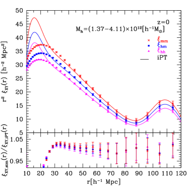
Figure 1: Top panel: Correlation functions of matter, halo, and their cross-correlation function at redshift $z=0$, multiplied by a factor of $r^{2}$. For the halo mass range, we consider $1.37\leq M_{\rm h}/(10^{12}{h}^{-1}M_{\odot})<4.11$ (Bin 1). The symbols are the results obtained from $N$-body simulations. The solid lines are the results of integrated perturbation theory (iPT) (Matsubara, 2011). Bottom panel: Ratio of correlation functions measured from $N$-body simulations to those from the iPT.

Before presenting the results for the cross-correlation coefficient, we compare the $N$-body simulation results with the iPT for the correlation functions themselves.

Figure 1 shows the results for the correlation functions of matter and halos, and their cross-correlation function at $z=0$. We use the halo catalog of “Bin 1” shown in Table 1. The amplitude of the halo-halo correlation is smaller than that of the matter-matter correlation, because the halo bias $b_{1}^{\rm E}$ in this halo range is 0.904 (less than 1). The error bars describe the 1-$\sigma$ error on the mean values obtained from 30 realizations. The error bars increase on large scales because of the finite size of the simulation box. The iPT predictions agree with $N$-body simulation results down to $r\sim$ 25$h^{-1}$Mpc within a few percent for all correlations. In Section V, we will see that a range of a few percent-level agreement in the cross-correlation coefficient is extended more than that in the correlation functions.

V Cross-Correlation Coefficient

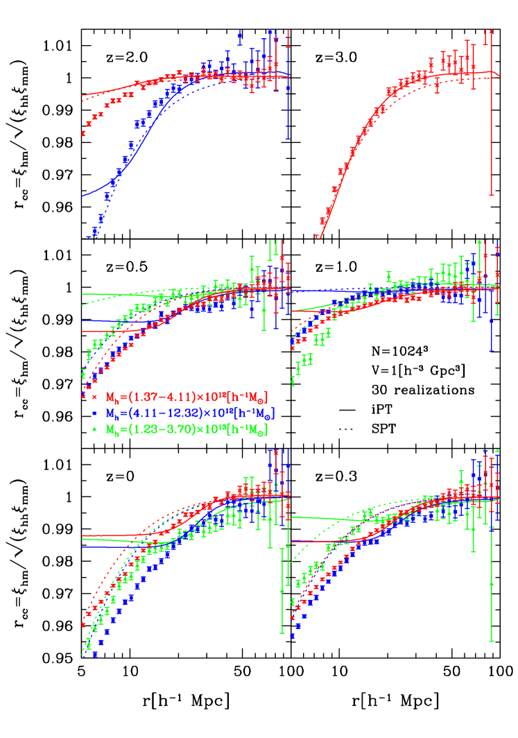
Figure 2: The cross-correlation coefficient between the matter and halo density fields at $z=0$, 0.3, 0.5, 1.0, 2.0, and 3.0. For the halo mass ranges, we consider $1.37\leq M_{\rm h}/(10^{12}{h}^{-1}M_{\odot})<4.11$ (Bin 1), $4.11\leq M_{\rm h}/(10^{12}{h}^{-1}M_{\odot})<12.32$ (Bin 2), and $1.23\leq M_{\rm h}/(10^{13}{h}^{-1}M_{\odot})<3.70$ (Bin 3). We do not plot the results in which the sum of the 1-$\sigma$ error bars in a range of $5\leq r_{i}/(h^{-1}{\rm Mpc})\leq 100$ is larger than 0.12, i.e., $\sum_{5\leq r_{i}\leq 100}\sigma_{i}>0.12$. The symbols are the results measured from $N$-body simulations. The solid lines are the results of integrated perturbation theory (iPT) (Matsubara, 2011) while the dotted lines are the results of the simple model derived from standard perturbation theory with local bias model (Equation 24). To empirically estimate $b_{1}$ and $b_{2}$, we use the relation in Equations (25) and (26) and then simply substitute $b_{1}^{\rm E}$ and $b_{2}^{\rm E}$ with $b_{1}$ and $b_{2}$.

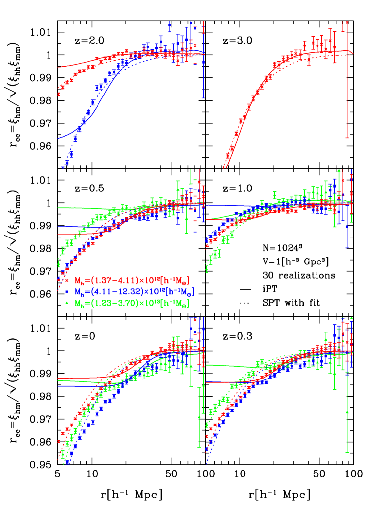
Figure 3: Same as Figure 2, but for the dotted lines, we fit $b_{2}/b_{1}$ to the $N$-body simulation results using a chi-square fit.

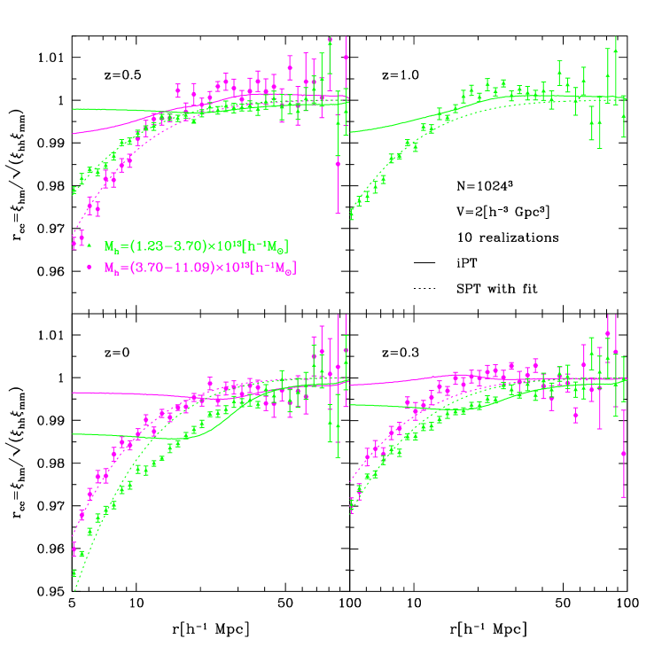
Figure 4: The cross-correlation coefficients with halo mass ranges $1.23\leq M_{\rm h}/(10^{13}{h}^{-1}M_{\odot})<3.70$ (Bin 4) and $3.70\leq M_{\rm h}/(10^{13}{h}^{-1}M_{\odot})<11.09$ (Bin 5), given at redshift $z=0$, 0.3, 0.5, and 1.0. We do not show the results in which the sum of the 1-$\sigma$ error bars in a range of $5\leq r_{i}/(h^{-1}{\rm Mpc})\leq 100$ is larger than 0.12. The triangle and circle symbols are the results of $N$-body simulations. The solid lines correspond to the results of integrated perturbation theory (iPT) (Matsubara, 2011) while the dotted lines correspond to results of standard perturbation theory with the fitted bias model (Equation 24).

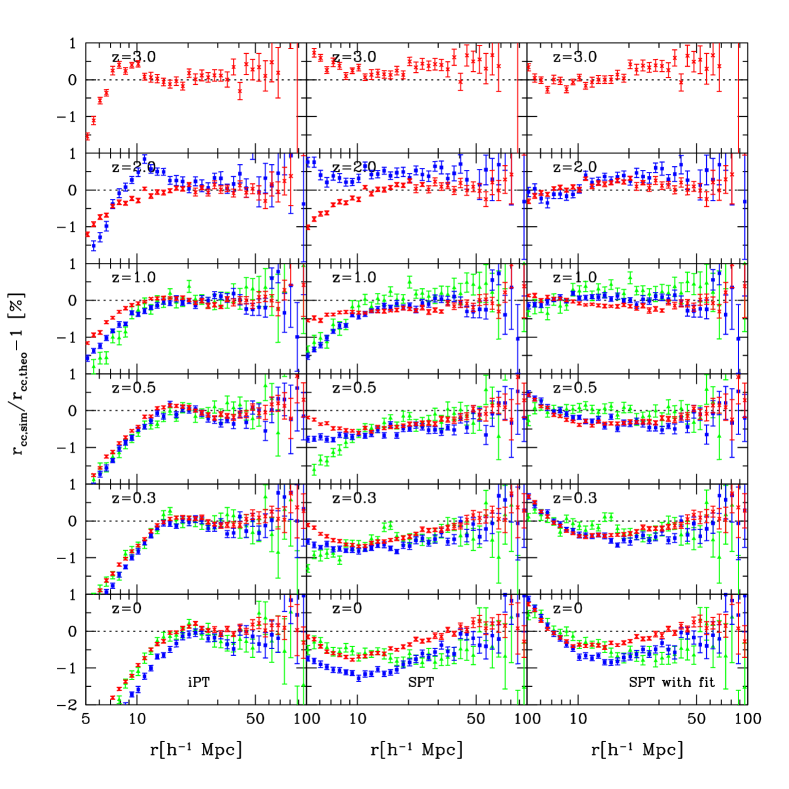
Figure 5: Fractional differences between $N$-body results and theoretical predictions are shown in percents, at redshifts $z=0$, 0.3, 0.5, 1.0, 2.0, and 3.0, from bottom to top. Left panels: iPT, Middle panels: SPT, and Right panels: SPT with fitting. The red cross, blue box, and green triangles are the results of Bin 1, 2, and 3.

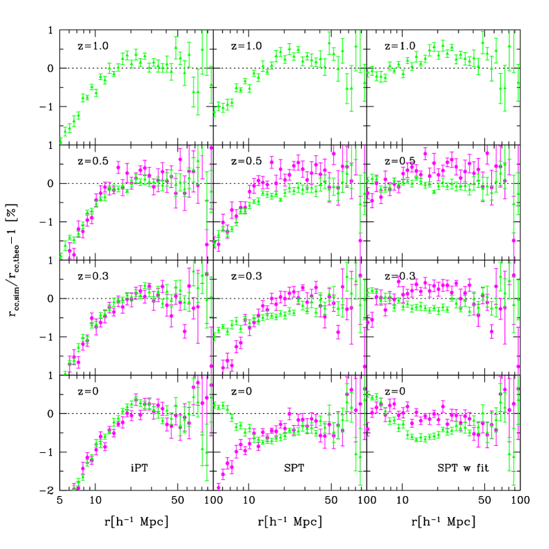
Figure 6: Same as Figure 5, but the results of Bin 4 (green triangle) and 5 (magenta circle) at $z=0$, 0.3, 0.5 and 1.0.

In the framework of the local biasing model, the density field of galaxies and their halos should be a stochastic function of the underlying dark matter density field (Dekel and Lahav, 1999). The stochasticity is very weak on large scales, while it becomes more important on small scales (Matsubara, 1999; Taruya and Suto, 2000; Yoshikawa et al., 2001; Cai et al., 2011).

One of the characteristic parameters of stochasticity is the cross-correlation coefficient between the matter and halo density fields, defined as

$$r_{\rm cc}(r)=\frac{\xi_{\rm hm}(r)}{\sqrt{\xi_{\rm mm}(r)\xi_{\rm hh}(r)}},$$ (23)

where $\xi_{\rm mm}(r)$, $\xi_{\rm hh}(r)$, and $\xi_{\rm hm}(r)$ are the matter and halo auto-correlation functions, and their cross-correlation function, respectively. The cross-correlation coefficient is the measure of the statistical coherence of the two fields (Pen, 1998; Tegmark and Bromley, 1999; Tegmark and Peebles, 1998; Seljak and Warren, 2004; Bonoli and Pen, 2009; Cacciato et al., 2012). If any scale-dependent, deterministic, linear-bias model is assumed, we have $r_{\rm cc}=1$. Therefore, deviations of the cross-correlation coefficient from unity would arise due to both the nonlinearity and stochasticity of bias.

Figure 2 shows the cross-correlation coefficient between the matter and halo density fields at $z=0$, 0.3, 0.5, 1.0, 2.0 and 3.0. The cross, square, and triangle symbols are the $N$-body simulation results measured from 30 realizations for halo masses $1.37\leq M_{\rm h}/(10^{12}{h}^{-1}M_{\odot})<4.11$ (Bin 1), $4.11\leq M_{\rm h}/(10^{12}{h}^{-1}M_{\odot})<12.32$ (Bin 2), and $1.23\leq M_{\rm h}/(10^{13}{h}^{-1}M_{\odot})<3.70$ (Bin 3), respectively. The error bars describe the 1-$\sigma$ error on the mean value obtained from 30 realizations. We do not plot the results in which the sum of the 1-$\sigma$ error bars in a range of $5\leq r_{i}/(h^{-1}{\rm Mpc})\leq 100$ is larger than 0.12, i.e., $\sum_{5\leq r_{i}\leq 100}\sigma_{i}>0.12$. It should be noted that halos in each bin are more biased as redshift increases, because we impose the same halo mass ranges for each bin. The solid curves show the iPT predictions. The iPT obtains good agreements with simulation results down to $r\sim$ 15$h^{-1}$Mpc within a range of error bars for all redshifts and halo mass ranges we have considered. Particularly at $z=3.0$, the iPT well reproduces the simulation result down to $r\sim$ 6$h^{-1}$Mpc. The deviations from unity in the cross-correlation coefficient $r_{\rm cc}$ on large scales are physical effects. Similar effects were also predicted even in a simple model of local bias by Scherrer and Weinberg (1998). The iPT prediction for the deviations has the same origin as theirs: the nonlinear dynamics on small scales nontrivially affect the cross coefficients on very large scales. Our simulations are consistent with these theoretical predictions. Below, we will see fractional differences between simulation results and theoretical predictions in Figure 5, to discuss the percentage error. The difference between the iPT and simulation results on small scales probably comes from the fact that the iPT breaks down on small scales (see, Figure 1) (Sato and Matsubara, 2011; Carlson et al., 2013). One can see that the iPT prediction on small scales is almost flat, unlike the simulation results. This is probably because the asymptotic behaviors of the correlation functions based on the iPT are almost the same (see Figure 1), and at any rate the iPT should not be applied on such small scales.

We also plot a simple model derived from Equations (21) and (22) as dotted curves and it is expressed as (Baldauf et al., 2010)

$$r_{\rm cc}(r)=1-\frac{1}{4}\left(\frac{b_{2}}{b_{1}}\right)^{2}\xi_{\rm L}(r),$$ (24)

by using the approximations $A(r)\ll\xi_{\rm NL}(r)$ and $B(r)\ll\xi_{\rm NL}(r)$.

To empirically estimate $b_{1}$ and $b_{2}$, we use general relations between local bias parameters in Lagrangian space and Eulerian space, which are derived in the spherical collapse model as (Matsubara, 2011)

$$b_{1}^{\rm E} =b_{1}^{\rm L}+1,$$ (25)

$$b_{2}^{\rm E} =\frac{8}{21}b_{1}^{\rm L}+b_{2}^{\rm L},$$ (26)

where $b_{1}^{\rm E}$ and $b_{2}^{\rm E}$ are Eulerian bias parameters. Note that both the Eulerian bias parameters $b_{n}^{\rm E}$ and the Lagrangian bias parameters $b_{n}^{\rm L}$ are local and independent of scales. In this phenomenological model, we simply substitute $b_{1}^{\rm E}$ and $b_{2}^{\rm E}$ with $b_{1}$ and $b_{2}$. To calculate $b_{1}^{\rm L}$ and $b_{2}^{\rm L}$, we use (Matsubara, 2008b)

$$b_{n}^{\rm L}=\frac{(-1)^{n}}{\delta_{c}^{n}}\frac{\displaystyle\int_{M_{1}}^{M_{2}}\nu^{n}\frac{{\rm d}^{n}f_{\rm MF}(\nu)}{{\rm d}\nu^{n}}\frac{{\rm d}\ln\sigma(M)}{{\rm d}{M}}\frac{{\rm d}{M}}{M}}{\displaystyle\int_{M_{1}}^{M_{2}}f_{\rm MF}(\nu)\frac{{\rm d}\ln\sigma(M)}{{\rm d}{M}}\frac{{\rm d}{M}}{M}}.$$ (27)

for halos in a mass range $M_{1}\leq M\leq M_{2}$. The simple model (Equation 24) with the above estimates of bias parameters shows better agreement with simulations for higher redshifts (i.e., more biased halos). We find that the cross-correlation coefficients of halos with $b_{1}^{\rm L}\gtrsim 2$ are well described in this method over all scales we considered. For lower redshifts (i.e., less biased halos), the simple model deviates more from the simulation results.

Meanwhile, when $b_{1}$ and $b_{2}$ are treated as free parameters, we fit $b_{2}/b_{1}$ to the simulation results using a chi-square fit. The result is shown as dotted lines in Figure 3. Other lines and symbols are the same as in Figure 2. Fittings are done in a range of $5\leq r/(h^{-1}{\rm Mpc})\leq 70$. In the fitting case, an improvement from the above empirical method is little for cases of high bias, but is important for cases of low bias. The simple model with fitted bias replicates the simulation results over all scales at $1\leq z\leq 3$. We can see that the cross-correlation coefficients estimated from $N$-body simulations have complicated behaviors in quasilinear regimes at low redshifts, which cannot be described in the simple model. We will describe percentage error later in Figure 5.

Figure 4 shows the results for the cross-correlation coefficient of large halos with mass ranges $1.23\leq M_{\rm h}/(10^{13}{h}^{-1}M_{\odot})<3.70$ (Bin 4) and $3.70\leq M_{\rm h}/(10^{13}{h}^{-1}M_{\odot})<11.09$ (Bin 5) at redshift $z=0$, 0.3, 0.5, and 1.0. The triangle and circle symbols are the simulation results of Bin 4 and Bin 5 estimated from 10 realizations of L2000. The solid and dotted lines are the predictions of the iPT and SPT with fitted bias, respectively. As in Figures 2 and 3, the iPT shows nice agreement with the simulation results on large scales even in large halo masses. The simple model with fitting also reproduces the simulation results for large halo masses. However, the fitting values of $b_{1}/b_{2}$ are not, in general, the same as those obtained from other statistics, such as the power spectrum and bispectrum, because $b_{1}$ and $b_{2}$ are renormalized.

To clarify how well theoretical models predict the $N$-body results, we plot fractional differences between $N$-body simulation results and theoretical predictions, $[r_{\rm cc,sim}(r)-r_{\rm cc,theo}(r)]/r_{\rm cc,theo}(r)$, as shown in Figures 5 and 6. These figures show that the iPT agrees with simulation results down to $r\sim$ 15 (10)$h^{-1}$Mpc within 0.5 (1.0) $\%$ for all redshifts and halo masses we considered. It should be noted that the iPT does not have any fitting parameter. The SPT with empirically determined bias reproduces $N$-body simulation results down to $r\sim$ 10$h^{-1}$Mpc within a percent-level for all redshifts except for $z=0$ (see, Figure 5). In the SPT with bias determined by fitting, a percent-level agreement is achieved over wide separation angles for all redshifts. However, the fitted parameters $b_{1}$ and $b_{2}$ are different from $b_{1}^{E}$ and $b_{2}^{E}$, which can be determined by other methods, e.g., the power spectrum and bispectrum.

VI Conclusion

In this paper, we have used 40 large cosmological $N$-body simulations of the standard $\Lambda$CDM cosmology to investigate the cross-correlation coefficient between the halo and matter density fields over a wide redshift range. The cross-correlation coefficient is crucial to extract information of the matter density field by combining galaxy clustering and galaxy-galaxy lensing measurements. Since the first attempt to detect galaxy-galaxy lensing (Tyson et al., 1984), its ability to constrain cosmological parameters has been shown (Mandelbaum et al., 2012).

We compared the simulation results with theoretical predictions of the iPT and simple models of bias with SPT. The iPT predicts the simulation results down to $r\sim$ 15 (10)$h^{-1}$Mpc within 0.5 (1.0) $\%$ for all redshifts and halo masses we considered. To improve the prediction, the two-loop correction to the iPT might be important. In the SPT with local bias model, bias parameters are renormalized and therefore they are determined empirically or treated as free parameters. The SPT with empirically determined biases with the spherical collapse model shows better agreement with simulations for more biased halos on small scales, although this model does not reproduce the complicated behaviors of the simulation results on quasilinear scales at low redshifts. The SPT with biases determined by fitting improves the predictions but the situation is almost the same at low redshift. Thus, the iPT accurately predicts the cross-correlation coefficient as long as quasilinear scales are considered.

Let us finally comment on convolution Lagrangian perturbation theory (CLPT), which was recently proposed by Carlson et al. (2013). The CLPT applies additional resummations on top of the simple LRT (restricted iPT with local Lagrangian bias), and its prediction significantly improves the simple LRT for the correlation function in real and redshift spaces on small scales. Therefore, it might be possible that the CLPT gives a better prediction for the cross-correlation coefficient between mass and halos and agrees with simulation results on small scales. Although it is important to examine how well the CLPT predicts these results, we leave it for future work.

In this paper we focused on fundamental features of bias stochasticity by the methods of numerical simulations and theoretical models. We believe the results of this paper could be a crucial first step to understand the galaxy biasing for future precision cosmology.